The prompt atmospheric neutrino flux in the light of LHCb

Abstract

The recent observation of very high energy cosmic neutrinos by IceCube heralds the beginning of neutrino astronomy. At these energies, the dominant background to the astrophysical signal is the flux of ‘prompt’ neutrinos, arising from the decay of charmed mesons produced by cosmic ray collisions in the atmosphere. In this work we provide predictions for the prompt atmospheric neutrino flux in the framework of perturbative QCD, using state-of-the-art Monte Carlo event generators. Our calculation includes the constraints set by charm production measurements from the LHCb experiment at 7 TeV, recently validated with the corresponding 13 TeV data. Our result for the prompt flux is a factor of about 2 below the previous benchmark calculation, in general agreement with other recent estimates, but with an improved estimate of the uncertainty. This alleviates the existing tension between the theoretical prediction and IceCube limits, and suggests that a direct detection of the prompt flux is imminent.

1 Introduction

The IceCube experiment Halzen:2010yj at the South Pole has recently made the first detection of high energy cosmic neutrinos from the Southern sky with deposited energies between 30 and 2000 TeV and arrival directions consistent with isotropy Aartsen:2013bka ; Aartsen:2013jdh ; Aartsen:2014gkd . Although these are mainly $\nu_{e}$ and $\nu_{\tau}$ charged-current and neutral-current (‘cascade’) neutrino interactions, the 37 events are consistent with expectations for equal fluxes of all three neutrino flavours Aartsen:2015ivb . Subsequently cosmic $\nu_{\mu}$ charged-current (‘track’) events have also been seen from the Northern sky Aartsen:2015rwa with comparable flux Aartsen:2015knd . At these high energies, the ‘conventional’ atmospheric neutrino flux, from the decays of pions and kaons produced by the collisions of cosmic rays with nuclei in the atmosphere Barr:2004br ; GonzalezGarcia:2006ay ; Honda:2006qj ; Honda:2011nf , is suppressed due to energy loss before the decays occur. However charmed mesons decay almost instantaneously and therefore, despite their smaller production cross-section, the ‘prompt’ neutrino flux from their decays ($\propto E_{\nu}^{-2.7}$) should dominate over the conventional flux ($\propto E_{\nu}^{-3.7}$) at high energies. Thus the prompt component is the most relevant background for the similarly hard spectrum expected for the astrophysical neutrino flux Halzen:2013dva ; Anchordoqui:2013dnh . Indeed the statistical significance ($5.7\sigma$) with which an atmospheric origin can be rejected for the 37 IceCube events is limited by the uncertainty in the expected atmospheric prompt neutrino flux.

Many calculations of the prompt neutrino flux have been presented Lipari:1993hd ; Pasquali:1998ji ; Enberg:2008te ; Gondolo:1995fq ; Martin:2003us ; Gelmini:1999ve ; Bhattacharya:2015jpa ; Engel:2015dxa ; Fedynitch:2015zma ; Arguelles:2015wba ; Garzelli:2015psa , however so far IceCube has not detected it and set only an upper limit of 1.52 times the central value of the benchmark ERS calculation Enberg:2008te at 90% CL Aartsen:2014muf . In a recent analysis this limit has been lowered further by a factor of 3 to only 0.54 times the above benchmark calculation Schoenen:2015ipa . This motivates a re-evaluation with state-of-the-art tools and inputs, providing, in particular, an improved estimate of all theoretical uncertainties. The major uncertainty is in the calculation of charm production at high-energies due to higher-order corrections and, especially, the imprecise knowledge of the gluon parton distribution function (PDF) at small-$x_{\text{Bjorken}}$. A recent breakthrough has been the availability of charm hadroproduction data from the LHCb experiment Aaij:2013noa ; Aaij:2013mga which covers the kinematical range directly relevant to the calculation of the atmospheric prompt neutrino flux.

With this motivation, we have recently validated state-of-the-art perturbative QCD calculations with the LHCb forward charm production data at 7 TeV Aaij:2013noa ; Aaij:2013mga , and included these measurements into the NNPDF3.0 global analysis Ball:2014uwa . We were thus able to construct a new PDF set, NNPDF3.0+LHCb, which is tailored for calculation of the prompt neutrino flux. We benchmarked three other codes, FONLL Cacciari:2001td , POWHEG Nason:2004rx ; Frixione:2007vw ; Alioli:2010xd and aMC@NLO Alwall:2014hca , finding good agreement both amongst themselves and with the LHCb data. Our calculations have subsequently been found to be in good agreement with the 13 TeV LHCb charm production data Aaij:2015bpa , which probe even smaller values of $x$.

In this work we calculate the atmospheric prompt neutrino flux using the canonical set of cascade equations implemented in the ‘$Z$-moment’ framework (see Enberg:2008te and references therein). Charm cross-sections and decays are obtained using the NLO Monte Carlo generator POWHEG with the NNPDF3.0+LHCb PDF set as input. We consider several parameterisations of the cosmic ray flux, including the most recent models Gaisser:2013bla ; Stanev:2014mla , and study the dependence of our result on the choice of input PDF set.

We compare our calculation with previous results, in particular the benchmark ERS calculation Enberg:2008te , as well as the recent BERSS Bhattacharya:2015jpa and GMS Garzelli:2015psa analyses. We emphasise that our calculation is the only one which is directly validated with LHCb data. All four calculations are consistent within our theoretical uncertainty band, with ERS being at the edge of the upper limit. Our central value is similar to the BERSS result, while the GMS result is a little higher. We also compare our result to the recent IceCube limit on the prompt neutrino flux, finding that our central value is consistent. Moreover our lower limit indicates that the prompt neutrino flux will soon be detected, thus enabling reliable subtraction of any contamination of the astrophysical neutrino candidates.

This paper is organised as follows. In § 2 we discuss the various inputs that enter the calculation of the prompt neutrino flux, including the parameterisations of the cosmic ray flux, the solution of the cascade questions, and the calculations of the various $Z$ moments. The results for the prompt flux are presented in § 3, where we compare with other recent determinations as well as with the latest IceCube limit. We also study the dependence of our result on the input PDF set and on the cosmic ray flux parameterisation. Our results are summarised in § 4 and are made publicly available in the form of an interpolation code which returns the prompt neutrino flux and its uncertainty for all adopted models of the cosmic ray flux.

2 Calculation of the prompt neutrino flux

First we present the parameterisations of the cosmic ray flux used in this work. We review the cascade equations for the propagation of particles in the atmosphere, and their solution using $Z$-moments. Then we discuss the calculation of the various $Z$-moments, with emphasis on the charm production cross-section and the associated theory uncertainties.

2.1 The incoming cosmic-ray flux

The flux of cosmic rays incident on the atmosphere is dominated by protons and has been measured by a variety of experiments (see recent reviews Seo:2012pw ; Kampert:2012mx ; Gaisser:2013bla ; Stanev:2014mla ). At energies $\gtrsim 10^{3}$ GeV relevant for calculating the prompt neutrino flux, a traditional parameterisation has been the broken Power Law (BPL) with a ‘knee’ at $E_{p}=5\times 10^{6}$ GeV, assuming all cosmic rays are protons:

$$\phi^{(0)}_{p}(E)=\begin{cases}1.7E_{p}^{-2.7}&{\rm GeV}\,{\rm sr}^{-1}\,{\rm cm}^{-2}{\rm s}^{-1},\qquad E_{p}\leq 5\times 10^{6}\,\,{\rm GeV}\\ 174E_{p}^{-3}&{\rm GeV}\,{\rm sr}^{-1}\,{\rm cm}^{-2}{\rm s}^{-1},\qquad E_{p}\geq 5\times 10^{6}\,\,{\rm GeV}\\ \end{cases}$$ (1)

Recently, more elaborate parameterisations of the cosmic ray flux have been provided, with emphasis on including composition data and improving the description above the ‘knee’ in the spectrum. One such set Gaisser:2011cc follows Hillas’ proposal Hillas:2006ms for accommodating three populations of cosmic rays: one associated with acceleration by supernova remnant shocks, a second galactic component from unspecified sources, and finally an extra-galactic component which dominates at the highest energies. The assumption is that 5 groups of nuclei, $i$, are contained in each of these three source components, $j$, such that the cosmic ray spectrum for the nuclear species $i$ can be written as

$$\phi^{(0)}_{i}(E)=\sum_{j=1}^{3}\left[a_{ij}\textit{ }E_{i}^{-\gamma_{ij}}\exp\left(-\frac{E_{i}}{Z_{i}R_{c,j}}\right)\right]\,,$$ (2)

where $R_{c,j}$ is the magnetic rigidity for the source component $j$, and $a_{ij}$ and $\gamma_{ij}$ are the corresponding normalization constants and spectral indices Gaisser:2011cc .

We construct an equivalent ‘all-proton’ spectrum by re-weighting the various nuclei:

$$\phi^{(0)}_{p,i}(E_{p})=A_{i}\times\phi^{(0)}_{i}(A_{i}E_{p})\ ,$$ (3)

with $A_{i}$ the atomic number of species $i$, and, to obtain the total cosmic ray flux, we sum over each of the 5 nuclear components:

$$\phi^{(0)}_{p}(E_{p})=\sum_{i=1}^{5}\phi^{(0)}_{p,i}(E_{i})=\sum_{i=1}^{5}\left[A_{i}\phi^{(0)}_{i}(A_{i}E_{p})\right]\ .$$ (4)

Thus we do not need to consider an effective nuclear attenuation length, since collective effects in nucleus-nucleus collisions can be safely ignored when calculating the nucleon interaction lengths inside the projectile. (Henceforth we drop the subscript $p$ on $E_{p}$ except when essential.)

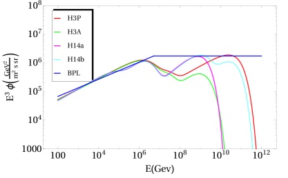
Figure 1: Comparison between the parameterisations of the cosmic ray flux used in this work.

We consider two types of ‘all-proton’ spectra, one where the third extra-galactic population contains contributions from all 5 nuclear groups, and another where only protons contribute, denoted respectively by H3A and H3P Gaisser:2011cc . These parameterisations have been extended Stanev:2014mla ; Gaisser:2013bla to include both additional heavy nuclear species, H14a, and to include a fourth population, H14b.

All the above spectra are compared in figure 1 with the flux rescaled by $E^{3}$ so that the region above the ‘knee’ is a horizontal line for the BPL spectrum and the difference from the other more recent parameterisations is emphasised. The latter are similar up to $\sim 10^{8}$ GeV, but differ significantly thereafter. Although now outdated, the results with the BPL spectrum are required for comparison with older calculations of the prompt neutrino flux.

2.2 The cascade equations and their solution

We now review the cascade formalism in the framework of the $Z$-moment approach Lipari:1993hd ; Gaisser:1990vg which is used to simulate the propagation of high energy particles and their decay products through the atmosphere. The aim is to solve a series of coupled differential equations dependent on the slant depth $X(l,\theta)$ measuring the atmosphere traversed by a particle:

$$X(l,\theta)\equiv\int_{l}^{\infty}\rho[h(l^{\prime},\theta)]\mathrm{d}l^{\prime}\,,$$

where $\rho$ is the density of the atmosphere dependent on the distance from the ground $l$ (along the particle trajectory) as well as on the zenith angle $\theta$. We adopt an isothermal model of the atmosphere, appropriate for atmospheric depths 10–40 km within which the bulk of particle production occurs:

$$\rho(h)=\rho_{0}\exp\left(-h/h_{0}\right)\,,\quad\rho_{0}=2.03\times 10^{-3}\,\,{\rm gm~{}cm}^{-3}\,,\quad h_{0}=6.4\,\,{\rm km}\,.$$ (5)

The horizontal depth of the atmosphere is $X\simeq 3.6\times 10^{4}~{}{\rm gm~{}cm}^{-2}$ while its vertical depth is $\simeq 1.3\times 10^{3}~{}{\rm gm~{}cm}^{-2}$. As in previous calculations, we are concerned with small angles about the vertical, $\theta\simeq 0$, where the conventional atmospheric neutrino flux arising from the decays of charged pions and kaons is the smallest.

For a particle of species $j$ and energy $E_{j}$ that has traversed a slant depth $X$, the cascade equation for the corresponding flux $\phi_{j}(E_{j},X)$ is

$$\frac{\mathrm{d}\phi_{j}}{\mathrm{d}X}=-\frac{\phi_{j}}{\lambda_{j}}-\frac{\phi_{j}}{\lambda_{j}^{\text{dec}}}+\sum_{k}S_{kj}(E_{j},X)\,,$$ (6)

where $\lambda_{j}$ is the interaction length, $\lambda_{j}^{\rm dec}$ is the decay length, and $S_{kj}$ are ‘(re)generation functions’ describing the production of particle $j$ from particle $k$ (where the sum includes $k=j$). This says that as a particle traverses the atmosphere, its flux will decrease when the particle undergoes an interaction (thus losing energy) or decays, as well as increase from the decay or interaction of other particle species. The (re)generation function is:

$$S_{kj}(E_{j},X)=\int_{E_{j}}^{\infty}\frac{\phi_{k}(E_{k}^{{}^{\prime}},X)}{\lambda_{k}(E_{k}^{{}^{\prime}})}\frac{\mathrm{d}n(k\rightarrow j;E^{{}^{\prime}}_{k},E_{j})}{\mathrm{d}E_{j}}\mathrm{d}E_{k}^{{}^{\prime}}\,,$$ (7)

where $\mathrm{d}n(k\rightarrow j;E^{{}^{\prime}}_{k},E_{j})$ is the differential transition rate between particle species $k$ and $j$. Assuming that the particle flux factorises into components dependent respectively on the energy $E$ and the slant depth $X$,

$$\phi_{k}(E,X)\equiv\phi_{k}(E)\times\widetilde{\phi}_{k}(X)\,,$$ (8)

it can be rewritten more simply as

$$S_{kj}(E_{j},X)=\frac{\phi_{k}(E_{j},X)}{\lambda_{k}(E_{j})}Z_{kj}(E_{j})\,,$$ (9)

with the key property that the moment $Z_{kj}$,

$$Z_{kj}(E_{j})=\int_{E_{j}}^{\infty}\frac{\phi_{k}(E_{k}^{{}^{\prime}},X)}{\phi_{k}(E_{j},X)}\frac{\lambda_{k}(E_{j})}{\lambda_{k}(E_{k}^{{}^{\prime}})}\frac{\mathrm{d}n(k\rightarrow j;E^{{}^{\prime}}_{k},E_{j})}{\mathrm{d}E_{j}}dE_{k}^{{}^{\prime}}\,,$$ (10)

is independent of the slant depth $X$ (which cancels in the ratio of fluxes).

Under this factorisation assumption, the cascade equations describing the flux of the various relevant species (protons $p$, mesons $m$, and leptons $l$) as they propagate through the atmosphere can be written as a set of coupled differential equations:

$$\frac{\mathrm{d}\phi_{p}}{\mathrm{d}X} =-\frac{\phi_{p}}{\lambda_{p}}+Z_{pp}\frac{\phi_{p}}{\lambda_{p}}\,,$$ (11)

$$\frac{\mathrm{d}\phi_{m}}{\mathrm{d}X} =-\frac{\phi_{m}}{\rho\mathrm{d}_{m}(E)}-\frac{\phi_{m}}{\lambda_{m}}+Z_{mm}\frac{\phi_{m}}{\lambda_{m}}+Z_{pm}\frac{\phi_{p}}{\lambda_{p}}\,,$$ (12)

$$\frac{\mathrm{d}\phi_{l}}{\mathrm{d}X} =\sum_{m}Z_{m\rightarrow l}\frac{\phi_{m}}{\rho d_{m}}\,,$$ (13)

where in the last equation the sum is restricted to the charmed hadrons that contribute to the prompt flux. Here $d_{m}(E)=c\beta\gamma\tau_{m}$ is the decay length of a particle with proper lifetime $\tau_{m}$.

Although the solution of these equations is in general quite involved, there are simple asymptotic solutions. The first equation for the proton flux (11) can be trivially integrated to give

$$\phi_{p}(E,X)=\phi^{(0)}_{p}(E)\exp\left(-X/\Lambda_{p}(E)\right)\,,$$ (14)

where we have defined the nucleon attenuation length as

$$\Lambda_{p}(E)\equiv\lambda_{p}(E)/(1-Z_{pp}(E))\,.$$ (15)

This depends in general on the nucleon’s interaction length in the atmosphere $\lambda_{p}(E)$:

$$\lambda_{p}(E)=\langle A\rangle/N_{0}\sigma_{pA}(E)\,,$$ (16)

where $\langle A\rangle=14.5$ is the average atomic number of air molecules, $N_{0}$ is Avogadro’s number, and the total inelastic air-nucleon cross-section is denoted by $\sigma_{pA}$.

Concerning the total proton-air cross-section, several parameterisations are available Kalmykov:1993qe ; Mielke:1994un ; Bugaev:1998bi ; Heck:1998vt ; Ahn:2009wx . We use the QGSJet0.1c model Mielke:1994un which fits available data well through the relevant energy range, including recent measurements made at the LHC Antchev:2011vs and the Pierre Auger Observatory Collaboration:2012wt . The prompt neutrino flux in fact depends very weakly on the modelling of $\sigma_{pA}(E)$ Garzelli:2015psa .

Given eq. (14) the cascade equation (12) for the meson flux can be solved by neglecting, in the low energy limit, the interaction and regeneration terms and, in the high energy limit, the decay terms. This yields two asymptotic solutions:

$$\phi_{m}^{\rm low}(E)=\phi_{p}^{(0)}(E)\frac{Z_{pm}(E)}{\Lambda_{p}(1-Z_{pp})}\rho d_{m}e^{-X/\Lambda_{p}}\,,$$ (17)

$$\phi_{m}^{\rm high}(E)=\phi_{p}^{(0)}(E)\frac{Z_{pm}(E)}{(1-Z_{pp})}\frac{(e^{-X/\Lambda_{m}}-e^{-X/\Lambda_{p}})}{1-\Lambda_{p}/\Lambda_{m}}\,,$$ (18)

where the dependence on the energy of the attenuation lengths $\Lambda_{p}$ and $\Lambda_{m}$ is implicit. Because of the additional dependence on the decay length in the low energy solution, these fluxes effectively scale with the proton flux (14) as follows:

$$\phi_{m}^{\rm low}(E)\propto E\phi_{p}(E)\,,$$ (19)

$$\phi_{m}^{\rm high}(E)\propto\phi_{p}(E)\,.$$ (20)

These intermediate solutions for meson fluxes are subsequently used as inputs in the corresponding low and high energy solutions for the leptonic decay of a meson $m\rightarrow l$, with either $l=\mu$ or $\nu$. The final vertical flux of leptons expected at the detector can then also be described by two asymptotic solutions, valid in the low– and high–energy regimes respectively:

$$\phi^{\rm low}_{l,m}(E) =\phi_{p}^{(0)}(E)\frac{Z_{pm}(E)}{1-Z_{pp}}Z^{\rm low}_{ml}(E)\,,$$ (21)

$$\phi^{\rm high}_{l,m}(E) =\phi_{p}^{(0)}(E)\frac{\epsilon_{m}}{E}\frac{Z_{pm}(E)}{1-Z_{pp}}\frac{\ln(\Lambda_{m}/\Lambda_{p})}{1-\Lambda_{p}/\Lambda_{m}}Z^{\rm high}_{ml}(E)\,.$$ (22)

where $\epsilon_{m}$ is a critical energy below which the probability of a meson to decay is greater than it is to interact:

$$\epsilon_{m}=\frac{m_{m}c^{2}h_{0}}{c\tau_{m}\cos\theta}\,.$$ (23)

The smaller the critical energy, the longer the decay length, hence the more energy the particle will lose by interactions in the atmosphere before it actually decays. In eqs. (21) and (22), $\phi_{l,m}$ represents the flux of lepton $l$ from the decays of the meson $m$.

Pions and kaons have a critical energy of $\mathcal{O}(10^{2})$ GeV. However, heavy quark mesons, such as $B$ and $D$, are characterised by much larger critical energies of $\mathcal{O}(10^{7})$ GeV and therefore mainly decay before losing energy in interactions with the atmosphere. This is why the ‘prompt’ neutrino flux from their decays is expected to dominate over the ‘conventional’ flux from $\pi,K$ at high energies. The contribution of $B$ mesons is usually neglected (despite a larger critical energy as compared to $D$ mesons) because the $b$-quark pair production cross-section is $<10\%$ of that of $c$-quark pairs up to $\sim 100$ PeV. However at such high energies, the contribution from D mesons would be damped as they start interacting before decaying, hence we show the prompt neutrino flux only up to $10^{7.5}$ GeV,

The final step in solving the cascade equations in the $Z$-moment approach is the geometrical interpolation of the low– and high–energy asymptotic solutions (21) and (22) which yields the final expression for the prompt lepton (neutrino) flux:

$$\phi_{l}(E)=\sum_{m}\frac{\phi_{l,m}^{\rm low}(E)\times\phi_{l,m}^{\rm high}(E)}{\phi_{l,m}^{\rm low}(E)+\phi_{l,m}^{\rm high}(E)}\,.$$ (24)

In the sum over mesons contributing to the prompt flux we include (the leptonic decays of) $D^{0}$, $\bar{D}^{0}$, $D^{\pm}$, $D_{s}^{\pm}$ and $\Lambda_{c}^{\pm}$. In fact $D^{0}$, $\bar{D}^{0}$, and $D^{\pm}$ account for the bulk of charm production in the atmosphere, with the other mesons contributing only around 10%.

2.3 Computation of the $Z$ moments

We need to compute the various $Z$-moments in order to evaluate the prompt flux (24), of which the most crucial is the nucleon to meson moment, $Z_{pm}$, which depends on the charm production cross-section in $pp$ collisions. We now discuss how to compute $Z_{ml}$, $Z_{pp}$, $Z_{mm}$ and $Z_{pm}$, and the corresponding theoretical uncertainties.

The generic $Z$-moment (10) defined earlier can be written for a (re)generation moment accounting for the interaction of a proton or a meson with an air nucleus, as

$$Z_{kj}(E_{j})=\int_{E_{j}}^{\infty}\frac{\phi_{k}(E_{k}^{{}^{\prime}},X)}{\phi_{k}(E_{j},X)}\frac{\lambda_{k}(E_{j})}{\lambda_{k}(E_{k}^{{}^{\prime}})}\frac{\mathrm{d}n(kA\rightarrow j;E^{{}^{\prime}}_{k},E_{j})}{\mathrm{d}E_{j}}\mathrm{d}E_{k}^{{}^{\prime}}\,,$$ (25)

while the decay moments that account for the leptonic decays of mesons are given by

$$Z_{ml}(E_{l})=\int_{E_{l}}^{\infty}\frac{\phi_{m}(E_{k}^{{}^{\prime}},X)}{\phi_{m}(E_{l},X)}\frac{d_{m}(E_{l})}{d_{m}(E_{k}^{\prime})}\frac{\mathrm{d}n(k\rightarrow l+X;E_{k}^{\prime},E_{l})}{\mathrm{d}E_{l}}\mathrm{d}E_{k}^{{}^{\prime}}\,.$$ (26)

Here the differential distributions $\mathrm{d}n(i\rightarrow f;E^{\prime},E)/\mathrm{d}E$ correspond to the number $n$ of final state particles $f$ with energies between $E$ and $E+\mathrm{d}E$ produced in an interaction where the initial state particle has energy $E^{\prime}$.

We now outline how each of the moments has been computed in this work:

$\bullet$ For the calculation of the leptonic decay moment $Z_{ml}$ (26), we use the fact that the energy distribution of leptons from charmed meson decays obeys a scaling law:

$$\mathrm{d}n(m\rightarrow l+X;E^{\prime},E)=F_{m\rightarrow l}\left(\frac{E}{E^{\prime}}\right)\frac{\mathrm{d}E}{E^{\prime}}\,,$$ (27)

where $F_{m\to l}(E)$ is the energy spectrum of the lepton $l$ from the decay of the meson $m$, computed in the rest frame of the latter. Defining the scaling variable $x_{E}=E/E^{\prime}$, we obtain

$$Z_{ml}(E)=\int_{0}^{1}\mathrm{d}x_{E}\frac{\phi_{m}(E/x_{E})}{\phi_{m}(E)}F_{m\rightarrow l}(x_{E})\,.$$ (28)

Exploiting the fact that the meson flux $\phi_{m}(E_{m})$ scales in the high–energy (19) and low–energy (20) limits we find that for the BPL cosmic ray spectrum, the leptonic moment reduces to a relatively simple expression

$$Z_{ml}(E_{l})=\int_{0}^{1}\mathrm{d}x_{E}\,\,x_{E}^{\beta}\,\,F_{m\rightarrow l}(x_{E})\,,$$ (29)

where the exponent is $\beta^{\rm low}=\{1.7,\,2\}$ in the low–energy solution, and $\beta^{\rm high}=\{2.7,\,3\}$ in the high-energy solution, for energies below and above the ‘knee’ respectively.

The calculation of the leptonic energy spectrum $F(x_{E})$ from charmed meson decays is performed with the Pythia8 Sjostrand:2014zea event generator and a boost is applied to transform $F(x_{E})$ from the laboratory to the meson rest frame. For the leptonic branching fractions of charmed mesons, we use the Particle Data Group recommended values  Agashe:2014kda for inclusive decays: $\mathcal{B}(D^{\pm}\rightarrow\nu_{l}X)=0.161$, $\mathcal{B}(D^{0}\rightarrow\nu_{l}X)=0.065$, $\mathcal{B}(D^{\pm}_{s}\rightarrow\nu_{l}X)=0.065$, and $\mathcal{B}(\Lambda_{c}^{\pm}\rightarrow\nu_{l}X)=0.028$. These values are adopted for both muon and electron neutrinos. The uncertainty on the branching fractions is well below 10% for $D^{0}$ and $D^{\pm}$, which are the most abundantly produced hadrons due to their large fragmentation fractions. Our result for the $Z_{ml}$ moments using the BPL cosmic ray spectrum are quite consistent with those reported earlier Gondolo:1995fq .

In figure 2 we compare the low-energy solution for the leptonic moment $Z^{\rm low}_{ml}(E)$ using the BPL cosmic ray spectrum for the four charmed mesons that contribute to the prompt flux, and where a sum over charge conjugate states is understood. Note that the decays of $D^{0}$ and $D^{\pm}$ contribute the bulk of the prompt leptonic flux. We also show a comparison of $Z^{\rm low}_{ml}(E)$ for $D^{\pm}$ only, using the different parameterisations of the cosmic ray flux to illustrate the large variations.

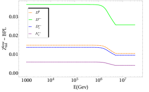
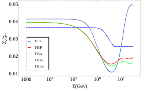
Figure 2: Left: Comparison of the leptonic moment $Z^{\rm low}_{ml}(E)$, assuming the BPL cosmic ray flux, for the four charmed mesons that contribute mainly to the prompt flux. Right: Comparison of the moment $Z^{\rm low}_{ml}(E)$ for $D^{\pm}$ mesons only for the 5 different parameterisations of the cosmic ray flux.

$\bullet$ When calculating the regeneration moments $Z_{pp}$ and $Z_{mm}$ that account for the interactions of protons and mesons in the atmosphere yielding a final state containing the same particle species, we follow previous studies Bhattacharya:2015jpa ; Garzelli:2015psa in adopting scaling laws for the proton-proton and meson-proton cross-sections, viz.

$$\frac{\mathrm{d}\sigma(pA\to p+X,E^{\prime},E)}{\mathrm{d}x_{E}} \simeq\sigma_{pA}(E)(1+n_{1})(1-x_{E})^{n_{1}}\,,$$ (30)

$$\frac{\mathrm{d}\sigma(mA\to m+X,E^{\prime},E)}{\mathrm{d}x_{E}} \simeq A^{3/4}\sigma_{Kp}(E)(1+n_{2})(1-x_{E})^{n_{2}}\,,$$ (31)

where, as before, $x_{E}=E/E^{\prime}$ is the fraction of the original energy retained by the incoming particle after interaction with an air nucleus in the atmosphere and the exponents are $n_{1}=0.51$ and $n_{2}=1.0$

Eq. (31) is based on the approximation that the cross-section for charmed meson scattering off nucleons can be related to the corresponding kaon-proton cross-section. The attenuation length of charmed mesons will be given under the same approximation as Pasquali:1998ji

$$\Lambda_{m}(E)\simeq\frac{A}{N_{0}\sigma_{pA}(E)}\frac{\sigma_{pp}(E)}{\sigma_{Kp}(E)}\frac{1}{(1-Z_{KK})}\,,$$ (32)

where the dependence of the kaon-proton cross-section on energy is from Agashe:2014kda .

In figure 3 we compare the proton and meson regeneration moments $Z_{pp}(E)$ and $Z_{KK}(E)$ for the 5 cosmic ray flux parameterisations. As for the leptonic moments, differences become appreciable only at high energies above the ‘knee’.

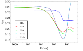
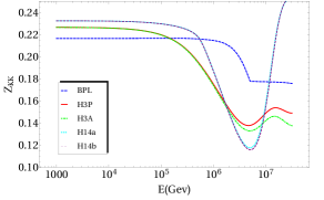
Figure 3: Left: Comparison of the proton regeneration moment $Z_{pp}(E)$ for the 5 cosmic ray flux parameterisations. Right: Same comparison, now for the meson regeneration moments $Z_{KK}(E)$.

$\bullet$ Finally we discuss the calculation of the proton-meson moment $Z_{pm}$, which is the main ingredient of the present work, as it contains the information on charm production in high energy collisions. The number distribution can be related to the differential charm production cross-section as:

$$\frac{\mathrm{d}n(pA\rightarrow h+X;E^{\prime},E)}{\mathrm{d}E}=\frac{1}{\sigma_{pA}(E^{\prime})}\frac{\mathrm{d}\sigma(pA\rightarrow h+X;E^{\prime},E)}{\mathrm{d}E}\,.$$ (33)

We assume that the charm production cross-section scales with the mean atomic number of air $\langle A\rangle$ as compared to the corresponding $pp$ cross-section

$$\sigma(pA\rightarrow D+X)\simeq\langle A\rangle\,\sigma(pp\rightarrow D+X)\,,$$ (34)

where $D$ is a generic charmed meson. This approximation is justified since even for forward $D$ production in $pPb$ collisions, the nuclear modification of the differential $D$ hadron cross-section results in a suppression of at most 10% Gauld:2015lxa . Although such effects are expected to increase in strength with atomic number, it is reasonable to ignore them when air is the target. This approximation is also supported by recent $B$ production data on $pPb$ collisions at the LHC Khachatryan:2015uja which show no evidence for nuclear modification effects.

Since we assume that ratios of fluxes are independent of the slant depth $X$ to first approximation, we can write down a simplified version of the $Z_{pm}$ moment (25) in terms of the charm production cross-section as follows:

$$Z_{pm}(E_{m})=\int_{E_{m}}^{\infty}\frac{\phi_{p}(E_{p}^{{}^{\prime}})}{\phi_{p}(E_{m})}\frac{\langle A\rangle}{\sigma_{pA}(E_{m})}\frac{\mathrm{d}\sigma(pp\rightarrow D+X;E^{{}^{\prime}}_{p},E_{m})}{\mathrm{d}E_{m}}\mathrm{d}E_{p}^{{}^{\prime}}\,,$$ (35)

Our calculation of the differential charm production cross-section in $pp$ collisions at high energies has been discussed in detail earlier Gauld:2015yia . As explained therein, it is based on perturbative QCD as implemented in the NLO Monte Carlo event generator POWHEG Alioli:2010xd , benchmarked with the corresponding FONLL Cacciari:2001td and aMC@NLO Alwall:2014hca calculations. The input PDF set is NNPDF3.0+LHCb Ball:2014uwa ; Gauld:2015yia , which includes the constraints on the small-$x$ gluon from the LHCb 7 TeV charm production cross-sections. The parton showering and fragmentation are modeled with Pythia8 Sjostrand:2014zea using the Monash 2013 tune Skands:2014pea . This is consistent with the semi-analytical fragmentation implemented in FONLL, tuned to LEP data Cacciari:2005uk . For the fragmentation probabilities, which describe the transition $f(c\to D)$ for the different types of charmed mesons, rather than using the default Pythia8 values we use the recent LHCb measurements Aaij:2013mga : $f(c\to D^{0})=0.565$, $f(c\to D^{\pm})=0.246$, $f(c\to D_{s}^{\pm})=0.080$, and $f(c\to\Lambda_{c})=0.094$.

Using this framework, we have computed the moment $Z_{pm}(E)$ for a wide range of energies, from $10^{3}$ to $10^{7.5}$ GeV. This requires the calculation of the charm production cross-section for incoming proton energies up to $E_{p}=10^{10.5}$ GeV in the laboratory frame. The POWHEG calculation is done in the center-of-mass frame for a wide range of $\sqrt{s}$ values, then boosted to the laboratory frame. In each case we have computed all the associated theoretical uncertainties from missing higher-orders, PDFs, and from the value of the charm mass Gauld:2015yia as follows:

• The charm quark pole mass is varied as $m_{c}=(1.5\pm 0.2)$ GeV,

• Renormalisation and factorisation scales are varied independently by a factor of 2 around the central scale $\mu_{0}=\sqrt{p_{T}+m_{c}^{2}}$, with the constraint $1/2<\mu_{F}/\mu_{R}<2$.

• PDF uncertainties are included at 68% CL,

• Finally the total theory uncertainty is obtained by addition in quadrature of these 3 components so may be considered as a crude ‘$1\sigma$’ band.

As with the other moments, the calculation of $Z_{pm}(E)$ is performed for all 5 cosmic ray flux parameterisations. In figure 4 we show the central theory prediction for $Z_{pm}(E)$ for the BPL spectrum for the four relevant charmed mesons (left plot) and then, for the $D^{0}$ and $\bar{D}^{0}$ mesons only, using all parameterisations (right plot).

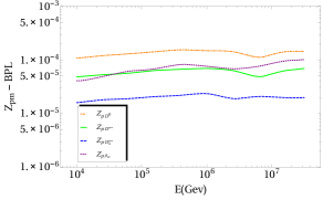
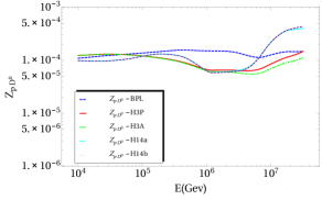
Figure 4: Same as figure 2 for the proton-meson moment $Z_{pm}(E)$.

3 Results

This section contains our main result, the updated calculation of the prompt neutrino flux. We discuss its dependence on the various inputs, in particular the adopted cosmic ray flux parameterisation and PDF set used. We compare our result with other recent calculations and also provide the spectral index of the prompt flux as a function of energy.

3.1 The prompt neutrino flux

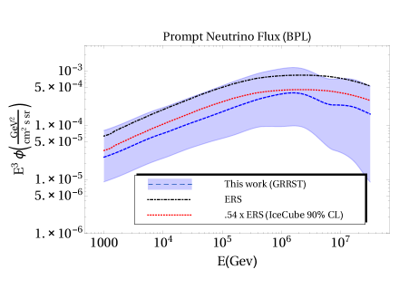
Figure 5: The prompt neutrino flux using the BPL cosmic ray spectrum as input. The error band includes all relevant sources of theoretical uncertainties: from PDFs (68% CL), missing higher orders and the charm mass, as discussed in the text. The ERS benchmark calculation Enberg:2008te is shown for comparison, as is the recent 90% CL upper limit on the prompt flux from IceCube Schoenen:2015ipa .

Figure 5 shows the prompt neutrino flux up to $10^{7.5}$ GeV using the BPL cosmic ray spectrum. Since PDF uncertainties have been substantially reduced using the LHCb data, the error band is dominated by the ‘scale uncertainties’ of the NLO perturbative QCD calculation which can be reduced only when the corresponding NNLO result is available Czakon:2015owf . However at energies above a PeV, PDF uncertainties still make an important contribution to the total error band. We also show the central value of the ERS calculation Enberg:2008te , which has been used as a benchmark in several IceCube analyses but is now in tension with the 90% CL upper limit labeled ‘0.54$\times$ERS’ Schoenen:2015ipa . The central value of our calculation is a factor of 2 smaller, and just below the IceCube limit on the prompt neutrino flux. Note that this limit should be interpreted with some care, since it depends e.g. on the specific parameterisation of the cosmic ray flux in the analysis.

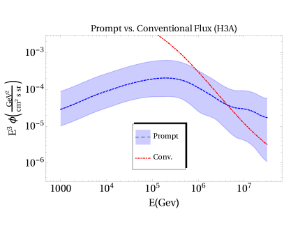
Figure 6: The prompt neutrino flux and its uncertainty using the H3A cosmic ray spectrum as input, compared to the conventional neutrino flux at IceCube Aartsen:2015xup .

In figure 6 we compare the prompt neutrino flux with the conventional neutrino flux from the decays of pions and kaons, using the same cosmic ray spectrum (H3A). We use the updated calculation Honda:2011nf for the South Pole location as implemented in the code NeutrinoFlux used by the IceCube collaboration Aartsen:2015xup . Whereas for the conventional flux the location of the experiment is important (as this determines the geomagnetic rigidity cut-off which filters incoming cosmic rays), this is irrelevant for the prompt flux which arises from the interaction of much higher energy cosmic rays). The cross-over energy where the prompt component begins to exceed the conventional one is about $4\times 10^{6}$ GeV.

As discussed in §. 2.1, an essential component of any calculation of the prompt neutrino flux is the parameterisation of the incoming cosmic ray flux, which is rather uncertain at the relevant high energies. Since cosmic rays with energies $\gtrsim(100-1000)E_{\nu}$ contribute to the prompt neutrino flux at a given $E_{\nu}$, a prediction of the prompt flux up to $10^{7.5}$ GeV requires knowledge of the cosmic ray flux up to at least $10^{10.5}$ GeV.

In figure 7 we compare our prediction for the prompt flux for all 5 parameterisations of the cosmic ray flux studied in this work: BPL, H3P, H3A, H14a and H14b. For energies $\lesssim 10^{7}$ GeV, the results for the 4 recent spectra are in reasonably good agreement with each other but consistently below the result with the BPL spectrum, with the maximal difference around $4\times 10^{6}$ GeV, where the BPL result is an order of magnitude larger. At very high neutrino energies $\gtrsim 10^{7}$ GeV, the recent H14 parameterisations Gaisser:2013bla ; Stanev:2014mla yield a prompt neutrino flux substantially larger than with the H3 parameterisations Gaisser:2011cc .

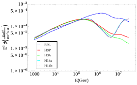
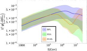
Figure 7: Left: Comparison of the central values of our calculation of the prompt neutrino flux for the 5 different parameterisations of the cosmic ray flux. Right: Comparison of the calculations including the theory uncertainty band for the BPL, H3A and H14b cosmic ray spectra.

In the right plot of figure 7 we perform a similar comparison, this time between the predictions using the BPL, H3A and H14b cosmic ray spectra, including in each case the corresponding theory uncertainty band (which has the same relative size in all cases, since it arises from the common input of the $Z_{pm}$ moment). It is clear that given these uncertainties, the results for the H3A and H14b parameterisations cannot be distinguished.

Another important input is the choice of PDF set, since knowledge of the PDF is required at low-$Q^{2}$ and very small-$x$ where experimental constraints are generally poor. In the present calculation, this uncertainty is substantially reduced by the use of the LHCb charm production data to constrain the small-$x$ gluon Gauld:2015yia . We now compare our baseline result for the prompt flux, obtained with the NNPDF3.0+LHCb PDF set (denoted by NNPDF3.0L), with the central prediction obtained using other PDF sets: ABM11 Alekhin:2012ig , CT14 Dulat:2015mca , HERAPDF1.5 H1:2015mha and MMHT14 Harland-Lang:2014zoa , in all cases at NLO. For each PDF set, the POWHEG calculation has been set up to include the required scheme modification terms; for instance, when $n_{f}=5$ PDFs are used as input, the scheme transformation terms from $n_{f}=3$ to $n_{f}=5$ are included Gauld:2015lxa ; Gauld:2015yia .

Results for the prompt flux using different PDF sets and the BPL cosmic ray spectrum are shown in figure 8 where the total theory uncertainty is shown for NNPDF3.0L only. All PDF sets yield results in good agreement, except for MMHT14 which yields a substantially larger flux at energies above $10^{5}$ GeV.

Thus the choice of PDF set is (with the exception of MMHT14) not important for the central value of the calculated flux. However it should be emphasised that the theory uncertainty band, which is shown here only for NNPDF3.0L, would have been much larger had we not included the LHCb charm hadroproduction data to reduce the uncertainty in the small-$x$ gluon Gauld:2015yia . Thus our estimate of the uncertainty in the prompt neutrino flux is more robust than for all other calculations to date, and accordingly we advocate its use for inferring a lower limit which can be used as a prior in analyses of experimental data.

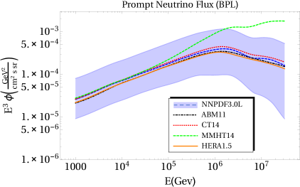
Figure 8: Comparison of our baseline calculation and its uncertainty using the NNPDF3.0L set Gauld:2015yia , with the corresponding central results using other PDFs as input: ABM11 Alekhin:2012ig , CT14 Dulat:2015mca , HERAPDF1.5 H1:2015mha and MMHT14 Harland-Lang:2014zoa . All calculations assume the BPL cosmic ray spectrum.

3.2 Comparison with previous calculations

In figure 9 we compare our result with the central values from the ERS Enberg:2008te , BERSS Bhattacharya:2015jpa and GMS Garzelli:2015psa calculations, all using the BPL cosmic ray flux as input. The relative differences would change only mildly if a different cosmic ray flux parameterisation was used as input.

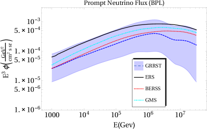
Figure 9: Comparison of our calculation (GRRST) with the central values from ERS Enberg:2008te , BERSS Bhattacharya:2015jpa and GMS Garzelli:2015psa , all calculated using the BPL cosmic ray spectrum.

The central values of these three previous calculations are contained within the total theory uncertainty band of our result. Our central value is close to BERSS, but systematically smaller than GMS, while the benchmark ERS result is at the upper end of the theory uncertainty band. Note that the BERSS calculation is based on the CT10 NLO PDF set Gao:2013xoa while the GMS calculation uses the ABM11 PDF set Alekhin:2012ig , neither of which incorporate the recent LHCb charm hadroproduction data. The ERS calculation was not based on pQCD at all, but the empirical ‘colour dipole model’. It is evident that there is now some stability in calculations of the prompt neutrino flux and that in particular a theoretical lower limit can be set (subject of course to the large systematic uncertainty in the parameterisation of the incoming cosmic ray flux).

3.3 Spectral index of the prompt neutrino flux

It is useful to extract the local spectral index of the prompt neutrino flux, defined as:

$$\gamma(E_{\nu})\equiv-\frac{d\ln\phi_{\nu}(E_{\nu})}{d\ln E_{\nu}}\,,\quad\text{where}\quad\phi_{\nu}(E_{\nu})=A(E_{\nu})\,E_{\nu}^{-\gamma(E_{\nu})}\,,$$ (36)

in order to compare with the standard expectation that $\gamma\simeq 2.7$. Both are shown in figure 10 which illustrates that above $10^{5}$ GeV the naïve scaling is not obeyed. The BPL, H3P and H3A cosmic ray fluxes all yield a a prompt neutrino spectrum which falls off more steeply, while with the H14a and H14b fluxes a harder spectrum is obtained (it is worth keeping in mind that at very high energies, above $\sim 50$ PeV, charmed mesons too will begin to lose energy by interaction with air nuclei before decaying, and at this point the fall-off of the prompt neutrino flux with $E_{\nu}$ will start to become similar to that of the conventional flux.).

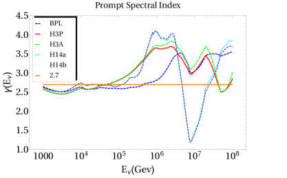
Figure 10: The effective spectral index $\gamma(E_{\nu})$ for the central value of our calculation of the prompt neutrino flux for all 5 parameterisations of the cosmic ray flux. For reference we show a line with $\gamma=2.7$, which is the usual expectation.

This indicates that a extraction of the prompt flux from a fit to data (including both the conventional flux and a cosmic signal) requires the full calculation of $\phi_{\nu}(E_{\nu})$ as a prior, with the overall normalisation left free but bounded by the total uncertainty band shown in figure 5. At a minimum, the lower limit on the prompt neutrino flux should be used as a prior, rather than allowing it to be zero as in current analyses Schoenen:2015ipa .

4 Outlook

We have presented predictions for the flux of prompt neutrinos arising from the decays of charmed mesons produced in the collisions of high energy cosmic rays in the atmosphere. Our calculation of charm production at high energy makes extensive use of NLO Monte Carlo event generators and parton distribution functions. The novelty of our approach is that it has been validated with the 7 TeV charm cross-sections measured by the LHCb experiment, and found to be consistent with the more recent 13 TeV measurements.

As input we have used the NNPDF3.0+LHCb PDF set, where the inclusion of the LHCb 7 TeV data substantially reduces the PDF uncertainties in the small-$x$ gluon. We include theory uncertainties arising from PDFs, missing higher-orders, and the value of $m_{c}$.

We have studied the dependence of our result on the choice of input cosmic ray fluxes, including the most recent parameterisations, and on the choice of input PDF set. Our predictions have been compared with other calculations, in particular with ERS Enberg:2008te , BERSS Bhattacharya:2015jpa and GMS Garzelli:2015psa . All three calculations are within the uncertainty band of our result, though our central value is the lowest. Our result is just consistent with the current experimental upper limit, suggesting that the prompt neutrino flux will be detected soon.

Our result for the prompt neutrino flux $\phi_{\nu}(E_{\nu})$ and its uncertainty, evaluated for 5 different input cosmic ray flux parameterisations, is available in terms of a C++ interpolation code from https://promptnuflux.hepforge.org. The interpolation tables can be used for neutrino energies between $10^{3}$ and $10^{7.5}$ GeV.

Since our calculations of charm hadroproduction have been validated with LHCb data, failure to detect the prompt neutrino flux in the range indicated would imply a flaw in the input assumptions, e.g. the cosmic ray flux parameterisation or possibly the $Z$-moment approach itself (e.g. the scalings in eqs. (30)-(32)). The latter can only be addressed by performing a full Monte Carlo simulation as in Gondolo:1995fq with updated QCD tools and data.

- (1) F. Halzen and S. R. Klein, IceCube: An instrument for neutrino astronomy, Rev. Sci. Instrum. 81 (2010) 081101, [arXiv:1007.1247].
- (2) IceCube Collaboration, M. Aartsen et al., First observation of PeV-energy neutrinos with IceCube, Phys.Rev.Lett. 111 (2013) 021103, [arXiv:1304.5356].
- (3) IceCube Collaboration, M. Aartsen et al., Evidence for high-energy extraterrestrial neutrinos at the IceCube detector, Science 342 (2013) 1242856, [arXiv:1311.5238].
- (4) IceCube Collaboration, M. Aartsen et al., Observation of high-energy astrophysical neutrinos in three years of IceCube data, Phys.Rev.Lett. 113 (2014) 101101, [arXiv:1405.5303].
- (5) IceCube Collaboration, M. G. Aartsen et al., Flavor Ratio of Astrophysical Neutrinos above 35 TeV in IceCube, Phys. Rev. Lett. 114 (2015), no. 17 171102, [arXiv:1502.03376].
- (6) IceCube Collaboration, M. G. Aartsen et al., Evidence for Astrophysical Muon Neutrinos from the Northern Sky with IceCube, Phys. Rev. Lett. 115 (2015), no. 8 081102, [arXiv:1507.04005].
- (7) IceCube Collaboration, M. G. Aartsen et al., A combined maximum-likelihood analysis of the high-energy astrophysical neutrino flux measured with IceCube, Astrophys. J. 809 (2015), no. 1 98, [arXiv:1507.03991].
- (8) G. Barr, T. Gaisser, P. Lipari, S. Robbins, and T. Stanev, A three-dimensional calculation of atmospheric neutrinos, Phys.Rev. D70 (2004) 023006, [astro-ph/0403630].
- (9) M. C. Gonzalez-Garcia, M. Maltoni, and J. Rojo, Determination of the atmospheric neutrino fluxes from atmospheric neutrino data, JHEP 10 (2006) 075, [hep-ph/0607324].
- (10) M. Honda, T. Kajita, K. Kasahara, S. Midorikawa, and T. Sanuki, Calculation of atmospheric neutrino flux using the interaction model calibrated with atmospheric muon data, Phys.Rev. D75 (2007) 043006, [astro-ph/0611418].
- (11) M. Honda, T. Kajita, K. Kasahara, and S. Midorikawa, Improvement of low energy atmospheric neutrino flux calculation using the JAM nuclear interaction model, Phys. Rev. D83 (2011) 123001, [arXiv:1102.2688].
- (12) F. Halzen, The highest energy neutrinos: first evidence for cosmic origin, Nuovo Cim. C037 (2014), no. 03 117–132, [arXiv:1311.6350]. [Astron. Nachr.335,507(2014)].
- (13) L. A. Anchordoqui et al., Cosmic Neutrino Pevatrons: A Brand New Pathway to Astronomy, Astrophysics, and Particle Physics, JHEAp 1-2 (2014) 1–30, [arXiv:1312.6587].
- (14) P. Lipari, Lepton spectra in the Earth’s atmosphere, Astropart.Phys. 1 (1993) 195–227.
- (15) L. Pasquali, M. Reno, and I. Sarcevic, Lepton fluxes from atmospheric charm, Phys.Rev. D59 (1999) 034020, [hep-ph/9806428].
- (16) R. Enberg, M. H. Reno, and I. Sarcevic, Prompt neutrino fluxes from atmospheric charm, Phys.Rev. D78 (2008) 043005, [arXiv:0806.0418].
- (17) P. Gondolo, G. Ingelman, and M. Thunman, Charm production and high-energy atmospheric muon and neutrino fluxes, Astropart.Phys. 5 (1996) 309–332, [hep-ph/9505417].
- (18) A. Martin, M. Ryskin, and A. Stasto, Prompt neutrinos from atmospheric and production and the gluon at very small x, Acta Phys.Polon. B34 (2003) 3273–3304, [hep-ph/0302140].
- (19) G. Gelmini, P. Gondolo, and G. Varieschi, Prompt atmospheric neutrinos and muons: NLO versus LO QCD predictions, Phys.Rev. D61 (2000) 036005, [hep-ph/9904457].
- (20) A. Bhattacharya, R. Enberg, M. H. Reno, I. Sarcevic, and A. Stasto, Perturbative charm production and the prompt atmospheric neutrino flux in light of RHIC and LHC, JHEP 06 (2015) 110, [arXiv:1502.01076].
- (21) F. Riehn, R. Engel, A. Fedynitch, T. K. Gaisser, and T. Stanev, Charm production in SIBYLL, arXiv:1502.06353.
- (22) A. Fedynitch, R. Engel, T. K. Gaisser, F. Riehn, and T. Stanev, Calculation of conventional and prompt lepton fluxes at very high energy, arXiv:1503.00544.
- (23) C. A. Arguelles, F. Halzen, L. Will, M. Kroll, and M. H. Reno, The high-energy behavior of photon, neutrino and proton cross sections, arXiv:1504.06639.
- (24) M. V. Garzelli, S. Moch, and G. Sigl, Lepton fluxes from atmospheric charm revisited, JHEP 10 (2015) 115, [arXiv:1507.01570].
- (25) IceCube Collaboration, M. G. Aartsen et al., Atmospheric and astrophysical neutrinos above 1 TeV interacting in IceCube, Phys. Rev. D91 (2015), no. 2 022001, [arXiv:1410.1749].
- (26) S. Schoenen, Talk at the IPA workshop, Madison, https://events.icecube.wisc.edu/getFile.py/access?contribId=89&sessionId=42&resId=0&materialId=slides&confId=68 .
- (27) LHCb Collaboration, R. Aaij et al., Measurement of B meson production cross-sections in proton-proton collisions at = 7 TeV, JHEP 1308 (2013) 117, [arXiv:1306.3663].
- (28) LHCb Collaboration, R. Aaij et al., Prompt charm production in pp collisions at sqrt(s)=7 TeV, Nucl.Phys. B871 (2013) 1–20, [arXiv:1302.2864].
- (29) NNPDF Collaboration, R. D. Ball et al., Parton distributions for the LHC Run II, JHEP 1504 (2015) 040, [arXiv:1410.8849].
- (30) PROSA Collaboration, O. Zenaiev et al., Impact of heavy-flavour production cross sections measured by the LHCb experiment on parton distribution functions at low x, Eur. Phys. J. C75 (2015), no. 8 396, [arXiv:1503.04581].
- (31) S. Alekhin et al., HERAFitter, Eur. Phys. J. C75 (2015), no. 7 304, [arXiv:1410.4412].
- (32) M. Cacciari, S. Frixione, and P. Nason, The p(T) spectrum in heavy flavour photoproduction, JHEP 0103 (2001) 006, [hep-ph/0102134].
- (33) P. Nason, A new method for combining NLO QCD with shower Monte Carlo algorithms, JHEP 0411 (2004) 040, [hep-ph/0409146].
- (34) S. Frixione, P. Nason, and C. Oleari, Matching NLO QCD computations with parton shower simulations: the POWHEG method, JHEP 0711 (2007) 070, [arXiv:0709.2092].
- (35) S. Alioli, P. Nason, C. Oleari, and E. Re, A general framework for implementing NLO calculations in shower Monte Carlo programs: the POWHEG BOX, JHEP 1006 (2010) 043, [arXiv:1002.2581].
- (36) J. Alwall, R. Frederix, S. Frixione, V. Hirschi, F. Maltoni, et al., The automated computation of tree-level and next-to-leading order differential cross sections, and their matching to parton shower simulations, JHEP 1407 (2014) 079, [arXiv:1405.0301].
- (37) LHCb Collaboration, R. Aaij et al., Measurements of prompt charm production cross-sections in collisions at = 13 TeV, arXiv:1510.01707.
- (38) T. K. Gaisser, T. Stanev, and S. Tilav, Cosmic Ray Energy Spectrum from Measurements of Air Showers, Front.Phys.China 8 (2013) 748–758, [arXiv:1303.3565].
- (39) T. Stanev, T. K. Gaisser, and S. Tilav, High energy cosmic rays: sources and fluxes, Nucl.Instrum.Meth. A742 (2014) 42–46.
- (40) E. S. Seo, Direct measurements of cosmic rays using balloon borne experiments, Astropart. Phys. 39-40 (2012) 76–87.
- (41) K.-H. Kampert and M. Unger, Measurements of the cosmic ray composition with air shower experiments, Astropart. Phys. 35 (2012) 660–678, [arXiv:1201.0018].
- (42) C. J. Todero Peixoto, V. de Souza, and P. L. Biermann, Cosmic rays: the spectrum and chemical composition from to eV, JCAP 1507 (2015), no. 07 042, [arXiv:1502.00305].
- (43) T. K. Gaisser, Spectrum of cosmic-ray nucleons, kaon production, and the atmospheric muon charge ratio, Astropart. Phys. 35 (2012) 801–806, [arXiv:1111.6675].
- (44) A. M. Hillas, Cosmic rays: Recent progress and some current questions, in Conference on Cosmology, Galaxy Formation and Astro-Particle Physics on the Pathway to the SKA Oxford, England, April 10-12, 2006, 2006. astro-ph/0607109.
- (45) T. K. Gaisser, Cosmic rays and particle physics. Cambridge University Press, 1990.
- (46) N. N. Kalmykov and S. S. Ostapchenko, The nucleus-nucleus interaction, nuclear fragmentation, and fluctuations of extensive air showers, Phys. Atom. Nucl. 56 (1993) 346–353. [Yad. Fiz.56N3,105(1993)].
- (47) H. H. Mielke, M. Foeller, J. Engler, and J. Knapp, Cosmic ray hadron flux at sea level up to 15 TeV, J. Phys. G20 (1994) 637–649.
- (48) E. Bugaev, A. Misaki, V. A. Naumov, T. Sinegovskaya, S. Sinegovsky, et al., Atmospheric muon flux at sea level, underground and underwater, Phys.Rev. D58 (1998) 054001, [hep-ph/9803488].
- (49) D. Heck, G. Schatz, T. Thouw, J. Knapp, and J. N. Capdevielle, CORSIKA: A Monte Carlo code to simulate extensive air showers, .
- (50) E.-J. Ahn, R. Engel, T. K. Gaisser, P. Lipari, and T. Stanev, Cosmic ray interaction event generator SIBYLL 2.1, Phys. Rev. D80 (2009) 094003, [arXiv:0906.4113].
- (51) G. Antchev et al., First measurement of the total proton-proton cross section at the LHC energy of =7 TeV, Europhys. Lett. 96 (2011) 21002, [arXiv:1110.1395].
- (52) Pierre Auger Collaboration, P. Abreu et al., Measurement of the proton-air cross-section at TeV with the Pierre Auger Observatory, Phys. Rev. Lett. 109 (2012) 062002, [arXiv:1208.1520].
- (53) T. Sjöstrand, S. Ask, J. R. Christiansen, R. Corke, N. Desai, et al., An introduction to PYTHIA 8.2, Comput.Phys.Commun. 191 (2015) 159–177, [arXiv:1410.3012].
- (54) Particle Data Group Collaboration, K. A. Olive et al., Review of Particle Physics, Chin. Phys. C38 (2014) 090001.
- (55) R. Gauld, Forward predictions for collisions, and sensitivity to cold nuclear matter effects, arXiv:1508.07629.
- (56) CMS Collaboration, V. Khachatryan et al., Study of B Meson Production in pPb Collisions at =5.02 TeV, arXiv:1508.06678.
- (57) R. Gauld, J. Rojo, L. Rottoli, and J. Talbert, Charm production in the forward region: constraints on the small-x gluon and backgrounds for neutrino astronomy, JHEP 11 (2015) 009, [arXiv:1506.08025].
- (58) P. Skands, S. Carrazza, and J. Rojo, Tuning PYTHIA 8.1: the Monash 2013 tune, European Physical Journal 74 (2014) 3024, [arXiv:1404.5630].
- (59) M. Cacciari, P. Nason, and C. Oleari, A study of heavy flavoured meson fragmentation functions in e+ e- annihilation, JHEP 0604 (2006) 006, [hep-ph/0510032].
- (60) M. Czakon, D. Heymes, and A. Mitov, High-precision differential predictions for top-quark pairs at the LHC, arXiv:1511.00549.
- (61) IceCube Collaboration, M. G. Aartsen et al., Measurement of the Atmospheric Spectrum with IceCube, Phys.Rev. D91 (2015) 122004, [arXiv:1504.03753].
- (62) S. Alekhin, J. Blümlein, and S. Moch, Parton distribution functions and benchmark cross sections at NNLO, Phys.Rev. D86 (2012) 054009, [arXiv:1202.2281].
- (63) S. Dulat, T. J. Hou, J. Gao, M. Guzzi, J. Huston, P. Nadolsky, J. Pumplin, C. Schmidt, D. Stump, and C. P. Yuan, The CT14 global analysis of quantum chromodynamics, arXiv:1506.07443.
- (64) ZEUS and H1 Collaboration, S. Schmidtt, Combination of measurements of inclusive deep inelastic scattering cross sections and QCD analysis of HERA data, arXiv:1506.06042.
- (65) L. Harland-Lang, A. Martin, P. Motylinski, and R. Thorne, Parton distributions in the LHC era: MMHT 2014 PDFs, Eur.Phys.J. C75 (2015), no. 5 204, [arXiv:1412.3989].
- (66) J. Gao, M. Guzzi, J. Huston, H.-L. Lai, Z. Li, P. Nadolsky, J. Pumplin, D. Stump, and C. P. Yuan, CT10 next-to-next-to-leading order global analysis of QCD, Phys. Rev. D89 (2014), no. 3 033009, [arXiv:1302.6246].