Reference by Description

Abstract

Messages often refer to entities such as people, places and events. Correct identification of the intended reference is an essential part of communication. Lack of shared unique names often complicates entity reference. Shared knowledge can be used to construct uniquely identifying descriptive references for entities with ambiguous names. We introduce a mathematical model for ‘Reference by Description’, derive results on the conditions under which, with high probability, programs can construct unambiguous references to most entities in the domain of discourse and provide empirical validation of these results.

1 Introduction

Messages often need to refer to real world entities. Communicating a reference to an entity is trivial when the sender and receiver share an unambiguous name for it. However, nearly all symbols in use are ambiguous and could refer to multiple entities. The word ‘Lincoln’ could for example, refer to the city, the president, or the film. In such cases, ambiguity can be resolved by augmenting the symbol with a unique description — ‘Lincoln, the President’. We call this Reference by Description. This leverages a combination of language (the possible references of ‘Lincoln’) and knowledge/context (that there was only one President named Lincoln) that the sender and receiver share to unambiguously communicate a reference.

This method of disambiguation is common in human communications. For example in the New York Times headline [17] ‘John McCarthy, Pioneer in Artificial Intelligence …’ the term ‘John McCarthy’ alone is ambiguous. It could refer to a computer scientist, a politician or even a novel or film. In order to disambiguate the reference, the headline includes the description “Pioneer in Artificial Intelligence”. An analysis, in the appendix, of 50 articles of different genres from different newspaper/magazine articles shows how ‘Reference by Description’ is ubiquitous in human communication.

The significance of correctly constructing and resolving entity references goes beyond human communication. The problem of correctly constructing and resolving entity references across different systems is at the core of data and application interoperability. The following example illustrates this.

Consider an application which helps a user select and watch a movie or TV Show. The application has a database of movies and shows, which the user can browse through, look at reviews from movie review sites such as RogerEbert.com, IMDb, Rotten Tomatoes and the other (language specific) sites. Then, it identifies a service (such as Amazon, Hulu, Netflix, …) from which the movie may be purchased or rented. Given that there are about 500,000 movies and 3 million TV episodes, one of the most difficult parts of building such an application is communicating references to these entities (movies and TV shows) with these different sites. Expecting a large number of different sites to use the same unique identifiers for these millions of entities is unrealistic.

Humans do not and cannot have a unique name for everything in the world. Yet, we communicate in our daily lives about things that do not have a unique name (like John McCarthy) or lack a name (like his first car). Our long term goal is to enable programs to achieve communication just as effectively. We believe that like humans, applications such as these too have to use ‘Reference by Description’.

The problem of entity reference is also closely related to that of privacy preserving information sharing. When the entity about whom information is shared is a person, and it is done without the person’s explicit consent (as with sharing of user profiles for ad targeting), it is critical this information not uniquely identify the person.

We are interested in a computational model of Reference by Description, which can answer questions such as: What is the minimum that needs to be shared for two communicating parties to understand each other? How big does a description need to be? When can we bootstrap from little to no shared language? What is the computational cost of using descriptions instead of unique names?

In this paper, we present a simple yet general model for ‘Reference by Description’. We devise measures for shared knowledge and shared language and derive the relation between these and the size of descriptions. From this, we answer the above questions. We validate these answers with experiments on a set of random graphs.

2 Background

Formal study of descriptions started with Frege [10] and Russell’s [22] descriptivist theory of names, in which names/identity are equivalent to descriptions. Kripke [16] argued against this position using examples where differences in domain knowledge could yield vastly different descriptions of the same entity. We focus not on the philosophical underpinnings of names/identity, but rather on enabling unambiguous communication between software programs.

In [23], the founding paper of information theory, Shannon referred to this problem, saying ‘Frequently the messages have meaning; that is they refer to or are correlated according to some system with certain physical or conceptual entities’, but he passed over it, saying ‘These semantic aspects of communication are irrelevant to the engineering problem.’

Computational treatments of descriptions started with linking duplicates in census records [25]. In computer science, problems in database integration, data warehousing and data feed processing motivated the development of specialized algorithms for detecting duplicate items, typically about people, brands and products. This work ([8], [4], [12] and [20]) has focused on identifying duplicates introduced by typos, alternate punctuation, different naming conventions, transcription errors, etc. Reference resolution has also been studied in computational linguistics, which has developed specialized algorithms for resolving pronouns, anaphora, etc.

Sometimes, we can pick a representation for the domain that facilitates reference by description. Keys in relational databases [6] are the best example of this.

The goal of privacy preserving information sharing [7] is the complement of unambiguous communication of references, ensuring that the information shared does not reveal the identity of the entities referred to in the message. [1], [18] discuss the difficulty of doing this while [15] shows how this can be done for search logs.

We have two main contributions in this paper. Most computational treatments to date have focused on specific heuristic algorithms for specific kinds of data. We present a general information theoretic model for answering questions like how much knowledge must be shared to be able to construct unambiguous references. Second, in contrast to previous treatments which use simple propositional / feature vector representations, we allow for richer, relational representations.

3 Communication model

We extend the classical information theoretic model of communication from symbol sequences to sets of relations between entities. In our model of communication (Fig. 1):

1. Messages are about an underlying domain. A number of fields from databases and artificial intelligence to number theory have modeled their domains as a set of entities and a set of N-tuples on these entities. We use this model to represent the domain. Since arbitrary N-tuples can be constructed out of 3-tuples [21], we restrict ourselves to 3-tuples, i.e., directed labeled graphs. We will refer to the domain as the graph, and the entities as nodes, which may be people, places, etc. or literal values such as strings and numbers. The graph has $N$ nodes.

2. The sender and receiver each have a copy of a portion of this graph. The arcs that the copies have could be different, both between them and from the underlying graph. The nodes are assumed to be the same.

3. The sender and receiver each associate a name (or other identifying string) with each arc label and zero or more names with each of the nodes in the graph. Multiple nodes may share the same name. Some subset of these names are shared.

4. Each message encodes a subset of the graph. We assume that the sender and receiver share the grammar for encoding the message.

5. The communication is said to be successful if the receiver correctly identifies the nodes that the message refers to.

When a node’s name is ambiguous, the sender may augment the message with a description that uniquely identifies it. Given a node $X$ in a graph, every subgraph that includes $X$ is a description of $X$. If a particular subgraph cannot be mistaken for any other subgraph, it is a unique description for $X$. The nodes, other than $X$, in the description are called ‘descriptor nodes’. In this paper, we assume that the number arc labels is much smaller than the number of nodes and arcs and that arc labels are unambiguous and shared.

Figures 2-4 illustrate examples of this model that are situated in the following context: Sally and Dave, two researchers, are sharing information about students in their field. They each have some information about students and faculty: who they work for and what universities they attend(ed). Fig. 1 illustrates the communication model in this context.

As the examples in Figures 2-4 illustrate, the structure of the graph and amount of language and knowledge shared together determine the size of unique descriptions. In this paper, we are interested in the relationship between stochastic characterizations of shared knowledge, shared language and description size. As discussed in the appendix, we can also approach this from a combinatorial, logical or algorithmic perspective.

In an earlier iterations of this paper [13] we presented this model and the solution for simpler version of this problem.

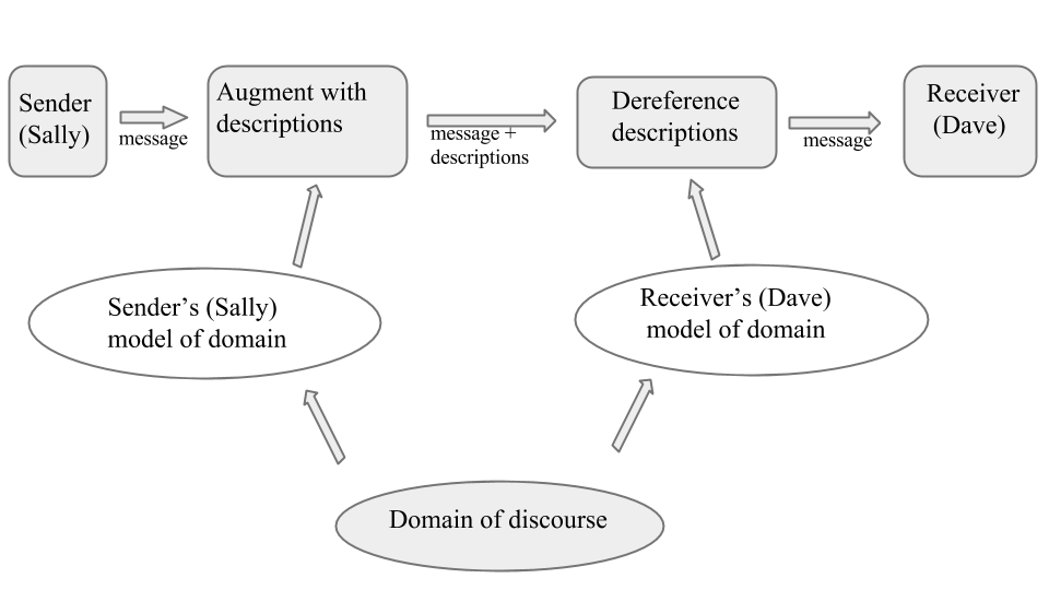
Figure 1: Communication model

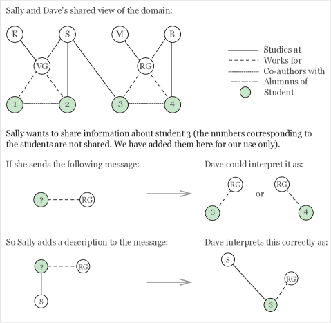
Figure 2: Flat message descriptions

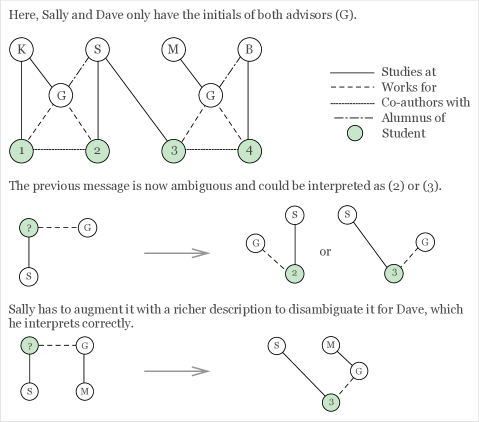
Figure 3: Deep message descriptions

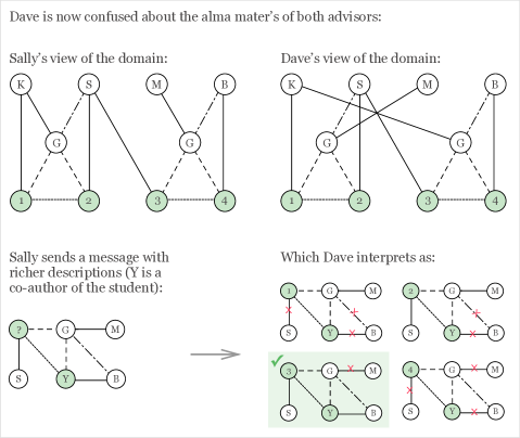
Figure 4: Sally has to augment her description with annotations of the co-author of the student (Y). Dave can use a process similar to decoding Hamming codes to deduce that she is most likely describing student (3).

4 Quantifying Sharing

When the sender describes a node $X$ by specifying an arc between $X$ and a node named $N_{1}$, she expects the receiver to know both which node $N_{1}$ refers to (shared language) and which nodes have arcs going to this node (shared domain knowledge). We distinguish between these two.

4.1 Shared Language / Linguistic Ambiguity

Let $p_{ij}$ be the probability of name $N_{i}$ referring to the $j\textsuperscript{th}$ object. The Ambiguity of $N_{i}$ is

$$A_{i}=\sum\limits_{j=0}^{N}-p_{ij}\log(p_{ij})$$

$A_{i}$ is the conditional entropy — the entropy of the probability distribution of over the set of entities given that the name was $N_{i}$. When there is no ambiguity in $N_{i}$, $A_{i}=0$. Conversely, if $N_{i}$ could refer to any node in the graph with equal probability, the ambiguity is $A_{i}=\log(N)$. Given a set of names in a message, if we assume that the intended object references are independent, the ambiguity rate associated with a sequence of names is the average of the ambiguity of the names. We use the Asymptotic Equipartition Property [5] to estimate the expected number of candidate referents of a set of names from from their ambiguity. The expected number of interpretations, of $\langle N_{1}N_{2}N_{3}\ldots N_{D}\rangle$ is $2^{DA_{d}}$.

Linguistic ambiguity may arise not just from a single name corresponding to multiple entities (like the earlier example of ‘Lincoln’) but also from variations of a name (such as ’Google Inc.’ vs ’Google’ or even ’Goggle’). Both these can be modeled with the definition of Ambiguity discussed here.

Typically, entities with more ambiguous names are described using entities less ambiguous names. We distinguish the ambiguity rate of the nodes being described ($A_{x}$) from that of the nodes used in the description ($A_{d}$).

4.2 Shared Domain Knowledge

Shared knowledge of the graph enables encoding/decoding of descriptions. Amount of sharing is not just a function of how much of the graph is shared, but the amount of information/knowledge in the graph. We want to characterize the information/knowledge content of the graph from the perspective of its ability to support distinguishing descriptions. We introduce Salience, a measure of how much differentiation is possible between nodes in the graph.

The classical measure for information (rate) is entropy. Let the adjancency matrix of the graph be generated by a process with entropy $H_{g}$. Then the information content of a sufficiently large randomly chosen set of $L$ arcs will be $LH_{g}$. However, given that the goal of our descriptions is to distinguish a given node ($X$) from other nodes, we do not want to randomly choose arcs involving the node. We would like to pick the arcs that are most likely to distinguish $X$. We now introduce a quantity, which we call ‘Salience’, to quantify the ability of the graph to generate distinguishing descriptions.

Given a graph $G$, there is an arc from a $X$ (the node being described) to each of the other nodes in the graph. Each of these $\langle arc-label,target\rangle$ pairs is a ‘statement’ about $X$. Each description of $X$ is a subset of the statements about $X$.

Given a particular set of $D$ nodes, $\langle D_{1},D_{2},D_{3},...D_{D}\rangle$, let the set of arcs from $X$ to these $D$ nodes be $\langle L_{XD_{1}},L_{XD_{2}},L_{XD_{3}}...L_{XD_{D}}\rangle$. Let the probability of this sequence (or more generally, ’shape’) occurring between these $D$ nodes and $any$ randomly chosen node in the graph be $p_{i}$. In Information Theoretic terms, the information content of this set of arcs, or this description, is $-\log p_{i}$. As $p_{i}$ decreases, the information content of the description and the likelihood of the description uniquely identifying $X$ increases. The Salience of a description its information content.

The information content of a description grows with its length. The ‘Salience Rate’ of a set of descriptions (or a single description) is the average salience of the descriptions in the ensemble divided by the average length (number of arcs) of the descriptions in the ensemble.

Consider an ensemble of size $S$ of descriptions, of average size $D$, that hold true for a given node $X$, containing $\gamma$ distinct shapes, with prior probabilities of holding true for a randomly chosen other node in the graph of $p_{1},p_{2},...p_{\gamma}$. Let the fraction of the $S$ descriptions that have these shapes be $q_{1},q_{2},...q_{\gamma}$ respectively. Assuming independence between the $p_{i}$, the Salience Rate ($F$) of the descriptions in this ensemble is:

$$F=\frac{1}{D}\sum_{i}-q_{i}\log p_{i}$$ (1)

Note that $p_{i}$ is not a distribution. The sum of the $p_{i}$’s in an ensemble may be less than 1. So, though the definition of salience bears superficial similarity to Cross entropy and Kullback-Liebler Divergence, they are different.

When the description (of $X$) is constructed by randomly selecting arcs that include $X$, the salience of the description is the entropy rate ($H_{g}$) of the adjacency matrix of the graph.

The salience of a description of an entity is a measure of how well it captures the most distinctive aspects of that entity. The salience of an ensemble is meaningful only in the context of the larger graph it is derived from. Since the $p_{i}$ depend on the rest of the graph, the same ensemble, relative to a different graph might have a different salience. For example, consider the following description: ‘X is a current US Senator, who studied at Harvard, …’. If the rest of the graph was about US senators, since many of the other nodes in the graph also satisfy this description, this description has a low salience. On the other hand, if the rest of the graph is about actors, this description has very high salience and uniquely identifies X.

A description with a higher salience is more likely to be unique. The sender may search through multiple candidate descriptions (of a given salience) to find a unique description. We are interested in an ensemble of $S$ candidate descriptions, at least one of which will be unique, with a probability of $1-\epsilon$, where $\epsilon$ can be made arbitrarity small. We will show later (equation 15) that for a given $\epsilon$, as $S$ increases, the required information content of the description decreases, up to a certain minimum. Beyond that, increasing $S$ does not reduce the required information content of descriptions. In other words, having more descriptions does not completely compensate for a lack of more informative descriptions. If we want at most a small constant number (independent of $N$) nodes to not have unambiguous descriptions, $S\propto\log N$.

Given our interest in constructing unique descriptions, we restrict our attention to ensembles that have the highest salience rate. We will use the symbol $F$ for the salience rate of an adquately large ($\log(N)$) ensemble with the highest salience rate. Given a description of length $L$ and $D$ nodes and a salience rate of $F$, the probability of a randomly chosen node satisfying this description is $2^{-LF}$.

Given a set of D nodes, we have only considered the arcs from X to these D nodes. We can extend our treatment to include some number, say $bD$ ($b<D/2$) arcs between the $D$ nodes in addition to the $D$ arc between $X$ and the $D$ nodes. The salience in such descriptions is the combination of the salience from $X$ to the $D$ arcs plus the salience from from the $bD$ arcs.

The salience of a graph is a measure of the underlying graph’s ability to provide unique descriptions. Differences in the view of the graph between the sender and receiver affect how much of this ability can be used. E.g., if ‘color’ is one attribute of the nodes but the receiver is blind, then the number of distinguishable descriptions is reduced. Some differences in the structure of the graph may be correlated. E.g., if the receiver is color blind, some colors (such as black and white) may be recognized correctly while certain other colors are indistinguishable. We use the mutual information between the sender’s and receiver’s versions of an ensemble as the measure of their shared knowledge. As before, consider an ensemble of size $S$ of descriptions, containing $\gamma$ distinct shapes. Let $P(x_{i})$ be the probability of the $i^{th}$ shape occurring between a randomly chosen node and a randomly chosen set of $D$ other nodes in the graph as seen by the sender. Given an ensemble, let $Q(x_{i})$ be the probability of the $i^{th}$ shape occurring in the ensemble. Let $P(y_{i})$ be the probability of the $i^{th}$ shape occurring between a randomly chosen node and a randomly chosen set of $D$ other nodes in the graph as seen by the sender. Given an ensemble, let $Q(y_{i})$ be the probability of the $i^{th}$ shape occurring in the ensemble. $P(y_{i}|x_{i})$ is the conditional probability of the receiver’s view having the $i^{th}$ relation between a randomly chosen node and $D$ descriptor nodes, given that it has this relation occurs in the sender’s view.

The sender chooses a description from the ensemble and sends it to the receiver (through a noiseless channel). The information content of the description to the receiver is not the same as it is to the sender. The information content of the description to the receiver is a function of the mutual information between the sender’s and receiver’s view of the underlying graph. Shared salience is defined as:

$$\text{Shared Salience}=\sum_{i}-Q(x_{i})Q(y_{i}|x_{i})\log P(x_{i})P(y_{i}|x_{i})$$ (2)

Shared salience is to salience as mutual information is to entropy. If the descriptions in an ensemble are constructed by randomly choosing statements or if the descriptions become very large, shared salience tends to the mutual information.

4.3 Salience of Random Graphs

Given our interest in probabilistic estimates on the sharing required, we focus on graphs generated by stochastic processes, i.e., Random Graphs. The most commonly studied Random Graph model is that proposed by Erdos and Renyi [9]. The Erdos-Renyi random graph $G(N,p)$ has $N$ nodes where the probability of a randomly chosen pair of nodes being connected is $p$. The Salience Rate of a sufficiently large $G(N,p)$ graph is $-\log(p)$ (or $-\log(1-p)$, whichever is larger).

More recent work on stochastic graph models has tried to capture some of the phenomenon found in real world graphs. Watts, Newman, et. al. [24], [19] study small world graphs, where there are a large number of localized clusters and yet, most nodes can be reach from every other node in a small number of hops. This phenomenon is often observed in social network graphs. ‘Knowledge graphs’, such as DBPedia [2] and Freebase [3], that represent relations between people, places, events, etc., tend to exhibit complex dependencies between the different arcs in/out of a node. Learning probabilistic models [11] of such dependencies is an active area of research.

$G(N,p)$ graphs assume independence between arcs, i.e., the probability of an arc $L_{i}$ occurring between two nodes is independent of all other arcs in the graph. Clustering and the kind of phenomenon found in knowledge graphs can be modeled by discharging this independence assumption and replacing it with appropriate conditional probabilities. For example, the clustering phenomenon occurs when the probability of two nodes $A$ and $C$ being connected (by some arc) is higher if there is a third node $B$ that is connected to both of them.

When the graph is generated by a first order Markov process, i.e., the probability of an arc appearing between two nodes is independent of other arcs in the graph, as in $G(N,p)$, calculating $F$ is simple. For more complex graphs where there are conditional dependencies between the arcs in/out from a node, we need to model the graph generating process as a second or even higher order Markov processes to compute $F$.

4.4 Description Shapes

The number of nodes ($D$) in a description of length ($L$) depends on its shape. The decoding complexity of a description is a function of both its size and its shape. Flat descriptions, which are the easiest to decode only use arcs between the node being described and the nodes in the description. E.g., Jim, who lives in Palo Alto, CA, age 56 yrs, works for Stanford, studied at UC Berkeley, married to Jane. The description consists of the arcs from node being described, Jim, to the descriptor nodes, Palo Alto CA, 56 yrs, Stanford, UC Berkeley and Jane. The length ($L$) flat descriptions, i.e., the number of arcs included, is the same as the number of nodes ($D$), i.e., $L=D$. They have $O(aD)$ decoding complexity, where $a$ is the average degree of each node.

Figure 5: Description Shapes

Flat descriptions are most effective when the descriptors have low ambiguity and do not require disambiguation themselves. In the previous description of Jim, the terms ‘Palo Alto, CA’, ‘Stanford’ and ‘UC Berkeley’ are relatively unambiguous. Most descriptions in daily communication are relatively flat. When low ambiguity descriptor terms are not available, the descriptor terms might need to be disambiguated themselves. In such cases adding ‘depth’ to the description is helpful.

In their most general form, deep descriptions do not impose any constraints on the shape. E.g., Jim, who is married to Jane who went to school with Jim’s sister and whose sister’s child goes to the same school that Jim’s child goes to. This description includes a number of links between the descriptor nodes (Jane, Jane’s school, Jim’s sister, etc.). The goal is capture some unique set of relationships that serve to unambiguously identify the node being described. Decoding deep descriptions involves solving a subgraph isomorphism problem and is NP-complete. These descriptions have length up to $L=D^{2}/2$ and have $O(N^{D})$ decoding complexity.

A trade off between decoding complexity and expressiveness can be achieved with by constraining the arcs (between descriptor nodes) that are included in the description. More specifically, the $D$ nodes in the description can be arranged into square blocks where only the arcs within each block are included in the description. We assume that there are $Db$ links between the descriptor nodes giving us $L=D(b+1)$. This is illustrated in Fig. 1, with the label ’intermediate’. When $b=D/2$, these reduce to the general form of deep descriptions.

5 Description size for unambiguous reference

Problem Statement: The sender is trying to communicate a message that mentions a large number of randomly chosen entities, whose average ambiguity is $A_{x}$. The overall graph has $N$ nodes. Each entity in the message has a description, involving on average, $D$ descriptor nodes, whose ambiguity rate is $A_{d}$. The description includes $bD$ ($b\leq D/2$) arcs between the descriptor nodes, which may be used to reduce the ambiguity in the descriptor nodes themselves, if any. We are interested in the average number of arcs and nodes required in the description.

In the most general terms, the ambiguity resolved by a description is less than or equal to its information content. More specifically, if $F$ is the salience rate of the graph, under the assumption of uniform salience rate, we have:

$$D=\frac{A_{x}}{F-\max(0,A_{d}-bF)}$$ (3)

Equation 33 covers a range of communication scenarios, some of which we discuss now. Proofs and empirical validation of equation 33 and its application to these scenarios are in the appendix We first examine the impact of the structure of the description, which affects the computational cost of constructing and decoding it.

5.1 Flat Descriptions

Flat descriptions (Fig. 2), which are the easiest to decode, only use arcs between the node being described and the descriptor nodes. They can be decoded in $O(aD)$, where $a$ is the average degree of a node. For flat descriptions, $b=0$, giving,

$$D=\frac{A_{x}}{F-A_{d}}$$    Flat descriptions (4)

Flat descriptions are very easy to decode, but require relatively unambiguous descriptor nodes, i.e., $F\gg A_{d}$. Most descriptions in human communication fall into this category.

5.2 Deep Descriptions

If the descriptor nodes themselves are very ambiguous ($F-A_{d}$ is small), the ambiguity of the descriptor nodes can be reduced by adding $bD$ arcs between them. If the descriptor nodes are considerably less ambiguous than the node being described ($A_{d}<A_{x}/2$), all ambiguity in the descriptor nodes can be eliminated by including $A_{d}/F$ links between them, giving us:

$$D=\frac{A_{x}}{F}$$    Deep descriptions (5)

Fig. 3 and 4 are examples of deep descriptions. Deep descriptions are more expressive and can be used even when the descriptor nodes are highly ambiguous. However, decoding deep descriptions involves solving a subgraph isomorphism problem and have $O(N^{D})$ decoding complexity.

5.3 Purely Structural Descriptions

When the sender and receiver don’t share any linguistic knowledge, all nodes are maximally ambiguious ($A_{x}=A_{d}=\log N$). We have to rely purely on the structure of the graph. We have:

$$D=2\log(N)/F$$ Purely structural descriptions (6)

By using detailed descriptions that include multiple attributes of each of the descriptor nodes, we can bootstrap communication even when there is almost no shared language.

5.4 Limiting Sender Computation

The sender may not be able to search through multiple candidate descriptions, checking for uniqueness. We are interested in $D$ such that every candidate description of size $D$ and salience rate $F$ is very likely unique. Assuming unambiguous descriptor nodes, we have:

$$D=\frac{\log(N)+A_{x}}{F}$$    Flat Landmark descriptions (7)

When the descriptions are constructed by randomly choosing facts about the entity, the salience rate is equal to the entropy of the adjacency matrix of the graph, $H_{g}$. In this case, the the nodes can use the same set of descriptor nodes, whence the name ‘landmark descriptions’.

5.5 Language vs Knowledge + Computation trade off

Consider a node with no name ($A_{x}=\log(N)$). Given a set of candidate descriptions with salience rate $F$, we consider two kinds of descriptions which are at opposite ends of the spectrum in the use of language vs knowledge. We could use purely structural descriptions (eq 6), which use no shared language. We could also, use a flat landmark description (eq. 34) which makes much greater use shared language and ignores most of shared graph structure/knowledge. Though the number of nodes $D=2\log(N)/F$ is the same in both, flat descriptions are of length $O(D)$, require no computation to generate and can be interpreted in time $O(aD)$. The former, in contrast are of length $O(D^{2})$. Further, since generating and interpreting them involves solving a subgraph isomorphism problem, they may require $O(N^{2\log(N)/F})$ time to interpret. This contrast illustrates tradeoff between shared language, shared domain knowledge and computational cost. We can overcome the lack of shared language by using shared knowledge, but only at the cost of exponential computation.

5.6 Minimum Sharing Required

When there are relatively unambiguous descriptor nodes available, $A_{x}/F$, the minimum size of the description for $X$, is a measure of the difficulty of communicating a reference to $X$. It can be high either because $X$ is very ambiguous ($A_{x}\to\log(N)$) and/or because very little unique is known about it ($F\to 0$). When $A_{x}/F\geq N$ it is not possible to communicate a reference to $X$. As the ambiguity of the descriptor nodes increases, domain knowledge has to play a greater role in disambiguation. In the limit, when there are no names, we have to use purely structural descriptions. In this case, $2\log(N)/F$ has to be less than $N$.

5.7 Non-identifying descriptions

We are interested in comparing the number of statements that can be made about an entity, while still keeping it indistinguishable from $K$ other entities [7], with the number of statements required to uniquely identify it. For this comparison to be meaningful, in both cases, we use statements with the same salience rate ($F$). Since the purpose is to hide the identity of the entity, its name is not included in the description, i.e., $A_{x}=\log(N)$. For flat descriptions we have:

$$D\leq\frac{\log(N)-\log(K)}{F-A_{d}}$$ (8)

Comparing this to equation 4 (with $A_{x}=\log(N)$), we see that there is only a small size difference ($\log(K)/(F-A_{d})$) between K-Anonymous descriptions and the shortest unique description. This is because of the phase change (discussed in the appendix), wherein at around $D=A_{x}/(F-A_{d})$, the probability of finding a unique description of size $D$ abruptly goes from $\approx 0$ to $\approx 1$. Though most descriptions of size $A_{x}/(F-A_{d})$ are not unique, for every node, there is at least one such description that is unique.

Given the statistical nature of equation 8, it is a neccessary, but not sufficient condition for privacy. Given a large set of entity descriptions, if the average size of description is close to or larger than this limit, then, with high probability, at least some of the entities have been uniquely identified.

6 Conclusion

As Shannon [23] alluded to, communication is not just correctly transmitting a symbol sequence, but also understanding what these symbols denote.

Even when the symbols are ambiguous, using descriptions, the sender can unambiguously communicate which entities the symbols refer to. We introduced a model for ‘Reference by Description’ and show how the size of the description goes up as the amount of shared knowledge, both linguistic and domain, goes down. We showed how unambiguous references can be constructed from purely ambiguous terms, at the cost of added computation. The framework in this paper opens many directions for next steps:

• Our model makes a number of simplifying assumptions. It assumes that the sender has knowledge of what the receiver knows. An example of this assumption breaking down is when two strangers speaking different languages have to communicate. It often involves a protocol of pointing to something and uttering its name in order to both establish some shared names and to understand what the other knows. A related problem appears in the case of broadcast communication, where different receivers may have different levels of knowledge, some of which is unknown to the sender. A richer model, that incorporates a probabilistic characterization of not just the domain, but also of the receiver’s knowledge, would be a big step towards capturing these phenomena.

• We have assumed large graphs and long messages. In practice, context is used to circumscribe the graph. Understanding the relation between context and descriptions would be very interesting.

• Though our communication model makes no assumptions about the graph, the simple form of the results presented here arise out of assumptions about ergodicity and uniformity of salience rate (which are analogous to those made in [23]). Versions of these results that don’t make these assumptions would be useful.

• Though we have touched briefly on practical applications of our model, much work remains to be done. The first task is the development of algorithms for constructing unique descriptions.

Appendices
We have the following appendices:

Appendix A:

Derivation of results and various special cases

Appendix B:

Empirical validation of results on random graphs

Appendix C:

Studies on usage of descriptive references on a set of newspaper/magazine articles

Appendix D:

Alternate problem formulations

Appendix 0.A Derivation of Results

0.A.1 Problem Statement

We are given a large graph $G$ with $N$ nodes and a message, which is a subgraph of $G$. The message contains a number of randomly chosen nodes. We construct descriptions for each of the nodes ($X$) in this subgraph so that it is uniquely identified. We are interested in a stochastic characterization of the relationship between the amount of shared domain knowledge, shared language, the number of nodes in the description ($D$) and the number of arcs ($L$) in the description.

For expository reasons, we go through the derivation for the simpler case, where there is no ambiguity in the descriptor nodes. We then extend this proof to the case where the descriptor nodes themselves may be ambiguous.

We model the graph corresponding to the domain of discourse, and the message being transmitted, as being generated by a stochastic processes. We carry over the assumption from Shannon [23] and information theory [5] that sequences of symbols (in our case, entries in the adjacency matrix) are generated by an ergodic process.

0.A.2 Unambiguous Descriptor Nodes

Consider a node $X$ in the message, which has an ambiguity of $A_{x}$. The description for $X$ involves $D$ unambiguous descriptor nodes. There are a number of possible configurations of $D$ arcs from $X$ to the descriptor nodes. Let us call these $\langle C_{XD1},C_{XD2},C_{XD3},...\rangle$. Let the probability of the $i^{th}$ of these occuring between a randomly chosen node a set of $D$ descriptor nodes be $p_{i}$.

The sender looks through an ensemble of $S$ descriptions, i.e., $S$ possible combinations of $D$ descriptor nodes in search of a unique description for $X$. Let the probability a randomly chosen element of this ensemble of these descriptions having the configuration $C_{XDi}$ be $q_{i}$.

There are $2^{A_{x}}-1$ nodes that might be mistaken for $X$. Consider one particular element in the ensemble that has the configuration $C_{XDi}$ with $X$. It provides a disambiguating description for $X$ if none of the $2^{A_{x}}-1$ nodes that we are trying to distinguish $X$ from is also in the configuration $C_{XDi}$ with this set of descriptor nodes. The probability of this is

$$(1-p_{i})^{2^{A_{x}}-1}$$ (9)

There are $S$ such sets of descriptors. We want the probability of none of these $S$ descriptions being unique to be less than $\epsilon$. Assuming independence between the descriptions in the ensemble, the probability of this is:

$$\prod_{D_{i}\in S}(1-(1-p_{i})^{2^{A_{x}}-1})\leq\epsilon$$ (10)

This product is over the candidate descriptions in the ensemble. Since we are interested in descriptions that are unlikely to be satisfied by other nodes, we can restrict our attention to the case where $p_{i}$ is very small, or more specifically, $(2^{A_{x}}-1)p_{i}\ll 1$. This allows us to use the binomial approximation, using which we get:

$$\prod_{D_{i}\in S}(1-(1-p_{i}(2^{A_{x}}-1)))\leq\epsilon$$ (11)

Assuming $2^{A_{x}}\gg 1$

$$\prod_{D_{i}\in S}p_{i}2^{A_{x}}\leq\epsilon$$ (12)

Taking logs,

$$\sum_{D_{i}\in S}\log p_{i}+SA_{x}\leq\log(\epsilon)$$ (13)

For sufficiently large $S$, the different description configurations will occur in proportion to their likelihood, i.e. the number of times shape $C_{XDi}$ occurs in the set $S$ is approximately $Sq_{i}$. So, $\sum_{D_{i}\in S}\log p_{i}$ can be rewritten as, $\sum_{j}Sq_{j}\log p_{j}$ where $j$ ranges over all the possible description configurations.

$$\sum_{D_{i}\in S}\log p_{i}=\sum_{j}Sq_{j}\log p_{j}=-SF_{D}$$ (14)

where $F_{D}$ is the average salience of the descriptions in the ensemble.

$$F_{D}\geq A_{x}-\frac{\log(\epsilon)}{S}$$ (15)

From this, we see that the impact of the size of $S$ on the average $F_{D}$ required is a function of $\epsilon$. Increasing $S$ beyond the stage where $\frac{\log(\epsilon)}{S}$ is sufficiently small does not provide additional benefit.

If we want at most a small constant (say one) node to not have a unique description, $\epsilon=1/N$, in which case we get,

$$F_{D}=A_{x}-\frac{\log(N)}{S}$$ (16)

If S is sufficiently large so that $\frac{\log(N)}{S}$ is negligible, we get,

$$F_{D}=A_{x}$$ (17)

If the salience rate of the ensemble is $F$, i.e., $FD=F_{D}$, where $D$ is the average length of the description in the ensemble, we have

$$D=A_{x}/F$$ (18)

This gives us an upper bound on $D$. We now show that this is also a lower bound (under the assumption, $A_{x}\gg 0$). To simplify, we demonstrate the proof for the average case, where $F_{D}=DF$. We are interested in large graphs where the number of ambiguous nodes does not grow with the size of the graph. So we let $\epsilon=1/N$. We can rewrite equation 28 as:

$$2^{(A_{x}-DF)S}=2^{(A_{x}+\frac{\log(N)}{S}-DF)S}$$ (19)

This is the number of ambiguous nodes. Let

$$D=\frac{(1+\delta)(A_{x}+\frac{\log(N)}{S})}{F}$$ (20)

where $\delta$ can be positive or negative. We get

$$2^{\delta(A_{x}+log(N)/S)S}=\text{Number of ambiguous nodes}$$ (21)

Clearly, for large $N$, the only way the number of ambiguous nodes does not grow with $N$ is if $\delta\leq 0$, showing that equation 33 is a lower bound as well.

A variant of this derivation shows the sensitivity of the whether a set of descriptions are unambiguous to the description size. Using the earlier approximations, we get the probability $p_{u}$ of a node having a uniquely identifying description of size $D$ as:

$$p_{u}=(1-(1-2^{-FD})^{2^{A_{x}}})^{S}$$ (22)

$$p_{u}=2^{(A_{x}-FD)S}$$ (23)

Let $D=\frac{A_{x}}{F}+\delta$, where $\delta$ can be positive or negative. This gives us

$$p_{u}=2^{\delta S}$$ (24)

Given the size of $S$ ($O(\log N)$), in the exponent, for large $N$, it is easy to see how as $\delta$ goes from negative to positive, at around $\delta=0$, there is a ‘phase change’ and $p_{u}$ abruptly goes from being $p_{u}\approx 0$ to $p_{u}\approx 1$. So, for a certain $D$ which is just less than given by equation 33 almost none of the nodes have unique descriptions. When the description size reaches that given by equation 33 there is an abrupt change and almost all nodes have unique descriptions.

If the shared salience between the sender and receiver is $M$, then, by using arguments identical to those in [23], we have

$$D=A_{x}/M$$ (25)

Note again that this is the upper bound on the average number of descriptor nodes for the entities in a sufficiently long message. When $A_{x}$ is low, description sizes will be small and individual nodes in the message may have shorter or longer descriptions. However, this bound still applies to the average description length for a large set of nodes.

0.A.3 Ambiguous Descriptor Nodes

We now consider the case where the descriptor nodes themselves are ambiguous. Let the ambiguity rate of the descriptor nodes be $A_{d}$. The description also includes $bD$ ($0\leq b\leq D/2$) arcs between the descriptor nodes. The role of these $bD$ arcs is to reduce the ambiguity of the descriptor nodes.

There are a number of possible configurations of $bD$ arcs between a randomly chosen set of $D$ candidate descriptor nodes. Let us call these $\langle C_{bD1},C_{bD2},C_{bD3}...\rangle$ Let the probability of the $i^{th}$ of these occurring amongst a randomly chosen set of $D$ descriptor nodes be $q_{i}$.

The sender looks through $S$ possible combinations of $D$ descriptor nodes in search of a unique description for $X$. Consider one particular set $i$ of $D$ descriptor nodes for $X$. Let the configuration of the arcs between $X$ and the $D$ nodes be $C_{XDi}$ and the configuration of the $bD$ arcs between the $D$ nodes be $C_{bDi}$.

There are $2^{DA_{d}}$ sets of $D$ nodes which have the same names as these descriptor nodes. Only one of these is the intended set of descriptor nodes. One of the other $2^{DA_{d}}-1$ sets of descriptor nodes can be mistaken for the intended descriptor nodes only if the $bD$ arcs between them also has the configuration $C_{bDi}$, the probability of which is $q_{i}$. Similarly, there are $2^{A_{x}}-1$ nodes that might be mistaken for $X$. The probability of one of these having the configuration $C_{XDi}$ with a set of $D$ descriptor nodes is $p_{i}$. This set of descriptor nodes provides a disambiguating description for $X$ if,

1. None of the $2^{A_{x}}-1$ nodes that we are trying to distinguish $X$ from is in the configuration $C_{XDi}$ with this set of descriptor nodes AND

2. None of the $2^{A_{x}}-1$ nodes that we are trying to distinguish $X$ from is in the configuration $C_{XDi}$ with one of the set of nodes that the descriptor nodes could be mistaken for.

The probability of this set of descriptor nodes providing a unique description for $X$ is:

$$(1-p_{i})^{2^{A_{x}}-1}(1-p_{i}q_{i})^{(2^{A_{x}}-1)(2^{DA_{d}}-1)}$$ (26)

As before, assume that $2^{A_{x}}\gg 1$. To simplify the analysis, we only consider the case where the ambiguity in the descriptor nodes is not insignificant, i.e., $2^{DA_{d}}\gg 1$. With these assumptions, we get:

$$(1-p_{i})^{2^{A_{x}}}(1-p_{i}q_{i})^{2^{A_{x}+DA_{d}}}$$ (27)

There are $S$ such sets of descriptors. The probability of none of these $S$ descriptions being unique should be less than $\epsilon$.

$$\prod_{D_{i}\in S}(1-(1-p_{i})^{2^{A_{x}}}(1-p_{i}q_{i})^{2^{A_{x}+DA_{d}}})<\epsilon$$ (28)

Using the binomial approximation (as before, we assume that the number of descriptions is large and hence $p_{i}$ and $p_{i}q_{i}$ are very small),

$$\prod_{D_{i}\in S}(1-(1-p_{i}2^{A_{x}})(1-p_{i}q_{i}2^{A_{x}+DA_{d}}))<\epsilon$$ (29)

Multiplying out, and ignoring terms with higher powers of $p_{i}$ and $q_{i}$,

$$\prod_{D_{i}\in S}p_{i}2^{A_{x}}\bigl{(}1+q_{i}2^{DA_{d}}\bigr{)}<\epsilon$$ (30)

Taking logs,

$$\sum_{D_{i}\in S}\log p_{i}+SA_{x}+\sum_{D_{i}\in S}\log(1+q_{i}2^{DA_{d}})<\epsilon$$ (31)

$q_{i}$ is the probability of the $i^{th}$ shape in the ensemble occurring between a randomly chosen set of $D$ nodes and is equal to $2^{-bDF}$, where $F$ is the salience rate for the ensemble with respect to the graph. So,

$$\sum_{D_{i}\in S}\log p_{i}+SA_{x}+\sum_{D_{i}\in S}\log(1+2^{DA_{d}-bDF})<\epsilon$$ (32)

Assume $\log(1+2^{DA_{d}-bDF})\approx D(A_{d}-bF),bF\leq A_{d}$. If $bF>A_{d}$, $\log(1+2^{DA_{d}-bDF})\approx 0$. So, $\log(1+2^{DA_{d}-bDF})\approx Dmax(0,A_{d}-bF)$. Letting $p_{i}=2^{-DF}$ as before, we get:

$$D\approx\frac{\log(N)/S+A_{x}}{F-max(0,A_{d}-bF)}$$ (33)

0.A.4 Searching through candidate descriptions

Description size (and hence decoding cost) is influenced by $S$, the number of potential descriptions the sender can search through. $S=1$ corresponds to the case where $D$ is sufficiently large, so that any selection of $D$ nodes will likely form a unique shape. This minimizes the sender’s computation at the expense of description length and receivers compute cost.

The $D$ nodes can be selected such that the same $D$ nodes are used to describe all the remaining $N-D$ nodes or each node can use a different set of $D$ nodes to describe it. We call these ‘landmarks’ nodes and the associated descriptions are called ‘landmark descriptions’. From eq. (33), we have:

$$D=\frac{\log(N)+A_{x}}{F-max(0,A_{d}-bF)}$$ (34)

Intuitively, the size of $D$ given by equation 34 answers the following question: how many randomly chosen facts, at the salience rate $F$, about an node does one have to specify to uniquely identify that node, with high probability. Note that in this case, the sender is not looking at the other nodes in the domain to see if the description is unique. If the description is longer that the size given by equation 34, it is very likely unique.

Remember that if the statements are chosen at random from the graph, the salience rate is $H_{g}$. So, restricting ourselves to flat descriptions composed of randomly chosen statements about the object, we have:

$$D=\frac{\log(N)+A_{x}}{H_{g}-A_{d}}$$ (35)

One interesting case of this is where the ‘randomly’ chosen nodes (in terms of which $X$ is described) is the same for all $X$. Such a set of descriptor nodes serve as ’landmarks’ in terms of which all other nodes are described. If the landmark nodes are unambiguous and the $X$ have no name, we have the special case where:

$$D=\frac{2\log(N)}{H_{g}}$$ (36)

At the other extreme, the sender could search through enough descriptions to find the smallest set of descriptor nodes for uniquely identifying $X$. For each description, the sender checks to see if the description is indeed unique. It is enough for the sender to search through $S$ randomly chosen descriptions such that $\frac{\log N}{S}\approx C$, where $C$ is a small constant (which can be ignored). In practice, by going through candidate descriptions in something better than random order, far fewer than $O(\log(N))$ descriptions need to be considered. In this case:

$$D=\frac{A_{x}}{F-max(0,A_{d}-bF)}$$ (37)

0.A.5 Flat Descriptions

The shape of the description influences decoding complexity. Flat descriptions, which are the easiest to decode, only use arcs between the node being described and the nodes in the description — no arcs between other nodes in the description are considered. Thus for these $b=0$.

$$D=\frac{A_{x}}{F-A_{d}}$$    Flat descriptions (38)

In the case where we do not have a name for the node being described, we get:

$$D=\frac{\log N}{F-A_{d}}$$    Flat descriptions (39)

As expected, flat descriptions are longer when the sender can not search through multiple candidates.

$$D=\frac{\log(N)+A_{x}}{F-A_{d}}$$    Flat landmark descriptions (40)

If $F<A_{d}$, we cannot use flat descriptions.

0.A.6 Deep Descriptions

When $A_{d}>0$, the number of nodes in the description may be reduced by using deep descriptions. In deep descriptions, in addition to the arcs between the descriptor nodes and $X$, arcs between the $D$ nodes may also be included in the description. We include $bD$ arcs between the descriptor nodes in the description.

We can restrict the search for descriptions (i.e., $S=1$), giving us deep landmark descriptions. If $b\leq\frac{A_{d}}{F}$, we have:

$$D=\frac{\log(N)+A_{x}}{(b+1)F-A_{d}}$$    Deep Landmark Descriptions (41)

Note that if $(b+1)F<A_{d}$, then communication will not be possible. When the descriptor nodes are unambiguous, adding depth does not provide any utility. For sufficiently large $S$,

$$D=\frac{A_{x}}{(b+1)F-A_{d}}$$    Deep Descriptions (42)

When $A_{d}<2A_{x}$ and $A_{d}/F<D/2$ and we can eliminate ambiguity in the descriptor nodes without increasing $D$, giving us:

$$D=\frac{A_{x}}{F}$$ Deep descriptions (43)

Given a particular $\langle F,A_{d},A_{x}\rangle$, deep descriptions have the fewest nodes. As $F$ decreases or $A_{x}$ (or $A_{d}$) increases, we need bigger descriptions.

0.A.7 Purely Structural Descriptions

For purely structural descriptions (i.e. no names), $A_{x}=A_{d}=\log N$. Allowing $b=D/2$ in equation 42:

$$D=\frac{\log(N)}{(D/2+1)F-\log(N)}\approx\frac{\log(N)}{DF/2-\log(N)}$$ (44)

$$D^{2}F=2D(1+\log(N))\approx 2D\log(N)$$ (45)

From which we get:

$$D=\frac{2\log(N)}{F}$$ (46)

0.A.8 Message Composition / Self Describing Messages

We have allowed for the entities in a message to be randomly chosen. The entities in the message may or may not have relations between them. For example, if the message is a set of census records or entries from a phone book, the different entities in the message will likely not be part of each other’s short descriptions. In contrast, in a message like a news article, the entities that appear do so because of the relations between them and can be expected to appear in each other’s descriptions.

We call messages, where all the descriptors for the entities in the message are other entities in the message, ‘self describing’ messages. We are interested in the size of such messages.

Let the message include the relationship of each node to all the other nodes. Setting $A_{x}=A_{d}$ in equation 41 and assuming $A_{d}/F<D/2$ and $A_{d}\ll\log(N)$, we get:

$$D=\frac{\log(N)}{F}$$ (47)

All messages with at least as many nodes as given by equation 47, that include all the relations between the nodes, are self describing.

Comparing eq. 34 to eq. 43 we see that while most sets of $A_{x}/F$ nodes do not have a unique set of relations, about $O(1/\log(N))$ of them do. Setting $b=D/2$ and $A_{x}=A_{d}=A$ in equation 42, and approximating, we get the minimum size of a self describing message:

$$D=\frac{2A}{F}$$ (48)

0.A.9 Communication Overhead

Descriptions can be used to overcome linguistic ambiguity, but at the cost of added computational complexity in encoding and decoding descriptions. We now look at the impact of descriptions on the channel capacity required to send the message. We only consider the case where the sender and receiver share the same view of the graph.

Consider a message that includes some number of arcs connecting $W$ nodes. If we assume that the number of distinct arc labels is much less than $N$, most of the communication cost is in referring to the $W$ nodes in the message.

Now, consider the case where each node in the graph is assigned a unique name. Each name will require $\log(N)$ bits to encode. If the message is a random selection of arcs from graph, we need $W\log(N)$ bits to encode references to the nodes.

Next consider encoding references to these $W$ nodes using flat descriptions with unambiguous landmarks where the descriptions are constructed by randomly picking statements about each node, i.e., $F=H_{g}$. This is the case covered by equation 36. We will need descriptions of length $2\log(N)/H_{g}$. These descriptions are strings from the adjacency matrix and have an entropy rate of $H_{g}$. So, the string of length $2\log(N)/H_{g}$ can be communicated using $2\log(N)$ bits and references to $W$ nodes will require $2M\log(N)$ bits. Comparing this to using unique names for each node, we see that there is a overhead factor of 2.

Now consider encoding references to these $W$ nodes using purely structural descriptions. These descriptions require $2\log(N)/H_{g}$ nodes and are of length $2(\log(N)/H_{g})^{2}$ and we will require $2\log(N)^{2}/H_{g}$ bits to represent each description, giving us an overhead of $2\log(N)/H_{g}$. We see that purely structural descriptions are not only very hard to decode, but they also incur a significant channel capacity overhead. This is assuming that the nodes in the message are randomly chosen. However, if the message is self describing, each of the nodes in the message serves as descriptors for the other nodes in the message, amortizing the description cost. Since there are $2\log(N)/H_{g}$ nodes in the message, there is no overhead.

0.A.10 Non-identifying descriptions

We are interested in the question of how much can be revealed about an entity without uniquely identifying it. This is of use in applications involving sharing data for research purposes, for delivering personalized content, personalized ads, etc.

We are interested in comparing the number of statements that can be made about an entity, while still keeping it indistinguishable from $K$ other entities [7], with the number of statements required to uniquely identify it. For this comparison to be meaningful, the descriptions need to be drawn from the same ensemble of descriptions. For a given salience rate $F$, we are interested in how big $D$ can be, such that at least $K$ other nodes satisfy this description. Since the purpose is to hide the identity of the entity, the name of the entity is not included in the description, i.e., $A_{x}=\log(N)$.

Given $N$ nodes and $R$ descriptions, assume that each node is randomly assigned a description. The probability that a given description corresponds to $r$ nodes is approximately:

$$p_{r}\approx\frac{e^{-\lambda}\lambda^{r}}{r!}$$ (49)

where $\lambda=\frac{N}{R}$, since this is a Poisson process with parameter $\lambda$. However, since there are $2^{DA_{d}}$ interpretations for $D$, let us find the number of other nodes that also map to these $2^{DA_{d}}$ descriptions. Since the sum of Poisson processes is a Poisson process, we find that the probability of $r$ additional nodes mapping to any of these $2^{DA_{d}}$ descriptions is

$$p_{r}\approx\frac{e^{-\lambda 2^{DA_{d}}}(\lambda 2^{DA_{d}})^{r}}{r!}$$ (50)

Thus the approximate number of nodes with fewer that $K$ such conflicts is

$$\sum_{r=0}^{K-1}Np_{r}=Ne^{-\lambda 2^{DA_{d}}}\sum_{r=0}^{K-1}\frac{(\lambda 2^{DA_{d}})^{r}}{r!}$$ (51)

We want this number to be a small constant $U$, thus

$$\sum_{r=0}^{K-1}\frac{(\lambda 2^{DA_{d}})^{r}}{r!}=\frac{Ue^{\lambda 2^{DA_{d}}}}{N}$$ (52)

The left hand side consists of the first $K$ terms of the Taylor series of $e^{x}$. Using Taylor’s theorem we have

$$e^{x}-\sum_{r=0}^{K-1}\frac{x^{r}}{r!}\leq\frac{e^{x}x^{K}}{K!}$$ (53)

Substituting the summation, we get:

$$e^{\lambda 2^{DA_{d}}}-\frac{Ue^{\lambda 2^{DA_{d}}}}{N}\leq\frac{e^{\lambda 2^{DA_{d}}}{(\lambda 2^{DA_{d}}})^{K}}{K!}$$ (54)

Thus

$$K!\biggl{(}1-\frac{U}{N}\biggr{)}\leq(\lambda 2^{DA_{d}})^{K}$$ (55)

Using Stirling’s approximation $K!\approx(K/e)^{K}$ and taking $K$-th roots of both sides,

$$\frac{K}{e}\biggl{(}1-\frac{U}{N}\biggr{)}^{\frac{1}{K}}\leq\lambda 2^{DA_{d}}$$ (56)

Since $U/N$ is small, we can use the binomial approximation to get

$$\frac{K}{e}\biggl{(}1-\frac{U}{KN}\biggr{)}=\frac{KN-U}{eN}\leq\frac{N2^{DA_{d}}}{F}$$ (57)

Thus $R\leq\frac{eN^{2}2^{DA_{d}}}{KN-U}$. Since $U\ll KN$, we can ignore $U$. For sufficiently large descriptions, on average, the probability of a description size $D$ holding for an object is $2^{-DF}$ where $F$ is the salience rate of the description. So, we have:

$$R=2^{DF}\leq\frac{eN2^{DA_{d}}}{K}$$ (58)

Taking logs we get:

$$D\leq\frac{\log N-\log\frac{K}{e}}{F-A_{d}}\approx\frac{\log N-\log K}{F-A_{d}}$$ (59)

0.A.10.1 Discussion on non-identifying descriptions

Comparing equation 59 to equation 39, we see that $D$ for ‘$K$-anonymity’ is very close to the $D$ for the shortest description of that node. For any node, there are a lot – ${N\choose D}$ – of descriptions of size $\frac{\log N-\log K}{F-A_{d}}$. All of these are satisfied by at least $K$ other nodes. In fact, we could use a slightly larger value of $D$, as given in equation 59 and most descriptions of this size would be satisfied by at least one other node. Most descriptions of size $\log N/(F-A_{d})$ do not reveal identity. But for every node, there is at least one description of this size that uniquely identifies it. Once the description size exceeds $2\log N/(F-A_{d})$, then, with high probability, every description of that size uniquely identifies the node.

This behavior of descriptions — until a certain size $D<\log N/(F-A_{d})$ they are, with high probability ambiguous, but once they cross that threshold, there is a ‘phase transition’ and their ambiguity cannot be guaranteed — follows from from the analysis in the earlier section on the phase transition in the likelihood of finding unique description of size $D$.

We also note that the limits we have derived are for the average length of descriptions for the entities in a sufficiently long message. Therefore, limits derived above are a neccessary, but not sufficient condition for anonymity. If the average size of the descriptions in a sufficiently large set of descriptions is higher than that given by equation 59, then, with high probability, anonymity has not been preserved.

Appendix 0.B Empirical Validation

We validate our results for description length for on a set of random graphs with different structural, connection and naming properties. We look at three kinds of random graphs:

1. Erdos-Renyi random graph with $N$ nodes, where the probability of two nodes being connected is $p$. Nodes are divided into two categories, the first are assigned names with ambiguity $A_{x}$ and the second are assigned names with ambiguity $A_{d}$.

2. A random bipartite graph where the probability of a node from one size (same number of nodes on both sides) being connected to a node from the other side is $p$. Nodes on one side are assigned names with ambiguity $A_{x}$ and nodes on the other side are assigned names with ambiguity $A_{d}$.

3. A random graph with local clustering, constructed as follows: We start with a number of Erdos-Renyi graphs that are not connected to each other. With then pick a number of pairs of nodes from different clusters and add a link between them, with probability $p$. Within each node, we divide nodes into two categories and assign them names with ambiguity $A_{x}$ and $A_{d}$.

We look at three categories of descriptions:

1. Flat descriptions with unambiguous descriptors (equation 18).

2. Flat descriptions with ambiguous descriptors (equation 38).

3. Deep descriptions (equation 42).

We vary the following parameters:

1. The salience rate for the graph. Note that the salience. rate for each of these graphs is $-log(p)$.

2. $A_{x}$, the ambiguity in the nodes being described.

3. $A_{x}$, the ambiguity in the descriptor nodes

For each value of $p$, $A_{x}$ and $A_{d}$, we generated 10 random instances of the graphs and (with $N=1000$). For each instance, computed the shortest description for 100 of the nodes. We compared the lengths of these descriptions with those predicted by the corresponding equations. Figures 2-9 compare the actual description lengths with those predicted by our theory.

Overall the predicted lengths correspond fairly closely to the observed lengths. The differences between observed and predicted lengths are because of the approximations made in deriving equations 18, 38 and 42.

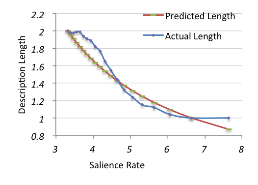
Figure 6: Description length as a function of salience, for flat descriptions with no ambiguity in descriptor nodes. Ambiguity in nodes being described is held constant at $\log_{2}100$ (i.e., 100 nodes corresponding to each name).

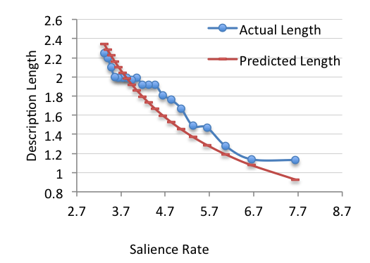
Figure 7: Description length as a function of salience, for flat descriptions. Ambiguity in nodes being described is held constant at $\log_{2}100$ (i.e., 100 nodes corresponding to each name). Ambiguity in descriptor nodes is $\log_{2}1.4$ (i.e., 1.4 nodes corresponding to each name, on average).

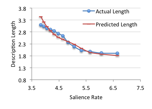
Figure 8: Description length as a function of salience, for deep descriptions. Ambiguity in nodes being described is held constant at $\log_{2}100$ (i.e., 100 nodes corresponding to each name). Ambiguity in descriptor nodes is $\log_{2}8$ (i.e., 8 nodes corresponding to each name, on average). Number of arcs between descriptor nodes ($bD$) comes from the actual graph.

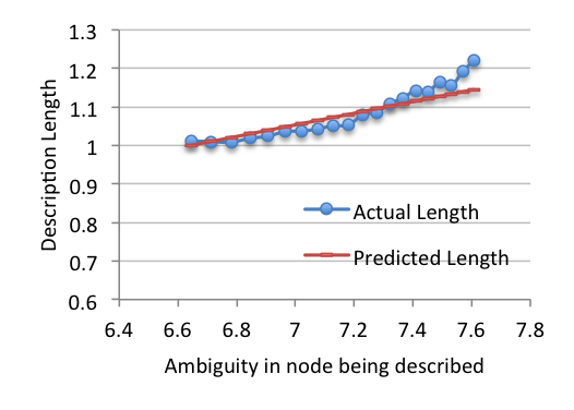
Figure 9: Description length as a function of ambiguity in nodes being described, for flat descriptions. Salience rate is held constant at $-\log_{2}0.01$ and there is no ambiguity in the descriptor nodes.

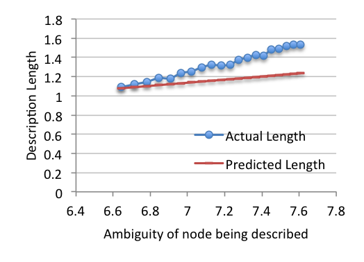
Figure 10: Description length as a function of ambiguity in nodes being described, for flat descriptions. Salience rate is held constant at $-\log_{2}0.01$. Ambiguity in descriptor nodes is $\log_{2}1.4$ (i.e., 1.4 nodes corresponding to each name, on average).

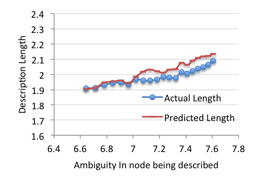
Figure 11: Description length as a function of ambiguity in the nodes being described, for deep descriptions. Salience rate is held constant at $-\log_{2}0.01$. Ambiguity in descriptor nodes is $\log_{2}10$ (i.e., 10 nodes corresponding to each name, on average). Number of arcs between descriptor nodes ($bD$) comes from the actual graph, which accounts for the jagged nature of the predicted length.

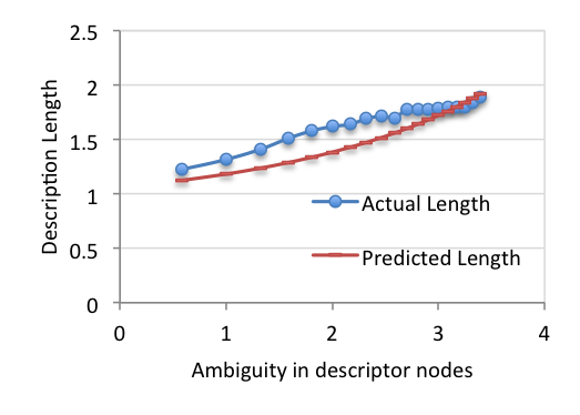
Figure 12: Description length as a function of ambiguity in the descriptor nodes, for flat descriptions. Salience rate is held constant at $-\log_{2}0.01$. Ambiguity in the nodes being described is held constant at $\log_{2}100$ (i.e., 100 nodes corresponding to each name, on average).

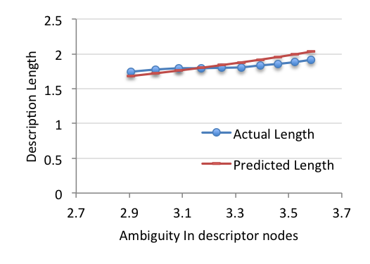
Figure 13: Description length as a function of ambiguity in the descriptor nodes, for deep descriptions. Salience rate is held constant at $-\log_{2}0.01$. Ambiguity in the nodes being described is held constant at $\log_{2}100$ (i.e., 100 nodes corresponding to each name, on average). Number of arcs between descriptor nodes ($bD$) comes from the actual graph.

Appendix 0.C Ubiquity of Reference by Description

Reference by description is ubiquitous in everyday human communication. Below are the results of an analysis of 50 articles from 7 different news sources, covering 3 different kinds of articles — analysis/opinion pieces, breaking news and wedding announcements/obituaries. We extracted the references to people, places and organizations from these articles. In each article entity pair, we examined the first reference in the article to that entity and analyzed it. The number of entities referenced and the size of descriptions, as measured by the number of descriptor entities in the description, are given in tables 1 and 2. We found the following:

1. Almost all references to people have descriptions. The only exceptions are very well known figures (e.g., Obama, Ronald Reagan).

2. References to many places, especially countries and large cities, do not have associated descriptions. References to smaller places, such as smaller cities and neighbourhoods follow a stylized convention, which gives the city, state and if neccessary, the country.

3. News articles tend to contain more references to public figures, who have shorter descriptions, reflecting the assumption of their being known to readers.

4. Wedding/obituary announcements, in contrast, tend to feature descriptions of greater detail.

5. The names of many organizations are, in effect, descriptions (e.g., Palo Alto Unified School District).

Article Type $\rightarrow$	Analysis/Opinion	Breaking	Obituaries	Total
Source $\downarrow$	Piece	News	Weddings
NY Times	23	6	24	53
BBC	14	24	4	42
Atlantic	121	0	0	121
CNN	10	11	6	27
Telegraph	12	20	10	42
LA Times	16	21	9	46
Washing. Post	28	23	8	59
Total	224	104	61	389

Table 1: Number of entity reference in each source, broken down by article type

Article Type $\rightarrow$	Analysis/Opinion	Breaking	Obituaries	Average
Source $\downarrow$	Piece	News	Weddings
NY Times	2.9	3	3.5	3.18
BBC	3	2.54	3.5	2.78
Atlantic	3.7	0	0	3.7
CNN	2.5	2.63	4	2.88
Telegraph	2.6	2.95	3.2	2.9
LA Times	2.43	2.52	3.55	2.69
Washing. Post	3.14	3.65	4	3.45
Average	3.29	2.92	3.57	3.23

Table 2: Average description size in each source, broken down by article type

Given that these articles are stories, the entities that are mentioned in them are closely related. Consequently, there exists no clear distinction between the parts of the description that serve to identify an entity from the message itself.

Appendix 0.D Alternate Problem Formulations

Descriptions based on random graph models are only one way of looking at the problem of Reference by Description. In this section, we briefly look at three alternate formulations. In all of these formulations, we continue to use the model described in section 3. We modify our analysis of descriptions and/or the richness of descriptions.

0.D.1 Combinatorial analysis

Here we look at descriptions from a combinatorial perspective. Variations exist for the following combinatorial decision problem: Given a graph with $N$ nodes, $B$ names and description size $D$, where each node is assigned one or zero of these names, does each node have a unique description, with fewer than $D$ nodes? In the worst case, $B=0$, in which case verification of a possible solution includes solving a subgraph isomorphism problem. Since subgraph isomorphism is known to be $NP$ complete, this problem is $NP$ complete. Since there are ${N\choose D}$ sets of $D$ nodes, we might need to solve as many subgraph isomorphism problems.

0.D.2 Descriptions and Logical Formulae

Here, we continue to model the domain of discourse as a directed labelled graph, but instead of restricting descriptions to subgraphs, we allow for a richer description language. More specifically, we use formulae in first order logic as descriptions.

Consider the class of descriptions where the node being described has no name ($A_{x}=\log(N)$), where some of the nodes in the description similarly have no name and others have no ambiguity. This class of descriptions can be represented as a first order formula with a single free variable (corresponding to the node being described) and some constant symbols (nodes with shared names). The formula is a unique descriptor for a node when the node is the only binding for the free variable that satisfies the formula. The simplest class of descriptions, ‘flat descriptions’, corresponds to the logical formula:

$$L_{x_{1}}(X,S_{1})\wedge L_{x_{2}}(X,S_{2})\wedge...\wedge L_{x_{S}}(X,S_{S})$$ (60)

where $L_{x_{i}}$ is the label of the arc between $X$ and the $i^{th}$ descriptor node.

Deep descriptions can be seen as introducing existentially quantified variables (corresponding to the descriptor nodes with no names) into the description. For the sake of simplicity, we consider graphs with a single label, $L$ (and $L_{null}$ indicating no arc). Consider a description fragment such as $L_{i}(X,S_{j})$, where $L_{i}$ is either $L$ or $L_{null}$. Let us allow a single nameless descriptor node. This corresponds to

$$(\exists y\ L_{i}(X,y)\wedge L_{i}(y,S_{j}))$$

Introducing two nameless descriptor nodes corresponds to

$$(\exists (y_{1},y_{2}) \ L_{i}(X,y_{1})\wedge L_{i}(X,y_{2})$$

$$\wedge L_{i}(y_{1},y_{2})\wedge L_{i}(y_{2},y_{1})$$

$$\wedge L_{i}(y_{1},S_{j})\wedge L_{i}(y_{2},S_{j}))$$

We can define different categories of descriptions by introducing constraints on the scope of the existential quantifiers. For example the nameless descriptor nodes can be segregated so that there are separate subgraphs relating the node being described to each of the shared nodes. The logical form of these descriptions (for a single nameless descriptor node) look like:

$$(\exists yL_{i}(X,y)\wedge L_{i}(y,S_{1}))$$

$$\wedge (\exists yL_{i}(X,y)\wedge L_{i}(y,S_{2}))$$

$$\wedge (\exists yL_{i}(X,y)\wedge L_{i}(y,S_{3}))\wedge\ldots$$

More complex descriptions can be created by allowing universally quantified variables, disjunctions, negations, etc. The axiomatic formulation also allows some of the shared domain knowledge to be expressed as axioms. The down side of such a flexible framework is that very few guarantees can be made about the computational complexity of decoding descriptions.

0.D.3 Algorithmic descriptions

We can allow descriptions to be arbitrary programs that take an entity (using some appropriate identifier that cannot be used in the communication) from the sender and output an entity (using a different identifier, understood by the receiver) to the receiver.

This approach allows us to handle graphs with structures/regularities that cannot be modeled using stochastic methods. An interesting question is the size of the smallest program required for a given domain, sender and receiver. If the shared domain knowledge is very low, the program will simply have to store a mapping from sender identifier to receiver identifier. As the shared domain knowledge increases, the program can construct and interpret descriptions.

References

- [1] C. C. Aggarwal. On k-anonymity and the curse of dimensionality. In Proceedings of the 31st international conference on Very Large Data Bases, pages 901–909, 2005.
- [2] C. Bizer, J. Lehmann, G. Kobilarov, S. Auer, C. Becker, R. Cyganiak, and S. Hellmann. Dbpedia-a crystallization point for the web of data. Web Semantics: science, services and agents on the world wide web, 7(3):154–165, 2009.
- [3] K. Bollacker, C. Evans, P. Paritosh, T. Sturge, and J. Taylor. Freebase: a collaboratively created graph database for structuring human knowledge. In 2008 ACM SIGMOD, pages 1247–1250. ACM, 2008.
- [4] W. W. Cohen, H. Kautz, and D. McAllester. Hardening soft information sources. In Proceedings of the sixth ACM international conference on Knowledge Discovery and Data mining, pages 255–259, 2000.
- [5] T. Cover and J. Thomas. Elements of Information Theory. Wiley-Interscience, 1991.
- [6] C. Data. An introduction to database systems. Addison-Wesley publ., 1975.
- [7] D. Dobkin, A. K. Jones, and R. J. Lipton. Secure databases: Protection against user influence. ACM Transactions on Database systems (TODS), 4(1):97–106, 1979.
- [8] A. K. Elmagarmid, P. G. Ipeirotis, and V. S. Verykios. Duplicate record detection: A survey. IEEE Transactions on Knowledge and Data Engineering, 19:1–16, 2007.
- [9] P. Erdős and A. Rényi. On random graphs. Publicationes Mathematicae Debrecen, 6:290–297, 1959.
- [10] G. Frege. Sense and reference. The philosophical review, pages 209–230, 1948.
- [11] L. Getoor, N. Friedman, D. Koller, and A. Pfeffer. Learning probabilistic relational models. In Relational data mining, pages 307–335. Springer, 2001.
- [12] L. Getoor and A. Machanavajjhala. Entity resolution: theory, practice & open challenges. Proceedings of the VLDB Endowment, 5(12):2018–2019, 2012.
- [13] R. V. Guha. Communicating and resolving entity references. CoRR, abs/1406.6973, 2014.
- [14] R. V. Guha and V. Gupta. Communicating semantics: Reference by description. CoRR, abs/1511.06341, 2015.
- [15] A. Korolova, K. Kenthapadi, N. Mishra, and A. Ntoulas. Releasing search queries and clicks privately. In Proceedings of the 18th international conference on World wide web, pages 171–180. ACM, 2009.
- [16] S. A. Kripke. Naming and necessity. Springer, 1972.
- [17] J. Markoff. John mccarthy, pioneer in artificial intelligence, dies at 84. New York Times, 2011.
- [18] A. Narayanan and V. Shmatikov. Myths and fallacies of personally identifiable information. Communications of the ACM, 53(6):24–26, 2010.
- [19] M. E. Newman and D. J. Watts. Scaling and percolation in the small-world network model. Physical Review E, 60(6):7332, 1999.
- [20] H. Pasula, B. Marthi, B. Milch, S. Russell, and I. Shpitser. Identity uncertainty and citation matching. In NIPS. MIT Press, 2003.
- [21] W. Quine. Mathematical logic. Harvard University Press, 1940.
- [22] B. Russell. On denoting. Mind, pages 479–493, 1905.
- [23] C. Shannon. The mathematical theory of communication. Bell System Technical Journal, 27:379–423, 1948.
- [24] D. J. Watts and S. H. Strogatz. Collective dynamics of ‘small-world’networks. nature, 393(6684):440–442, 1998.
- [25] W. E. Winkler. The state of record linkage and current research problems. In Statistical Research Division, US Census Bureau. Citeseer, 1999.