HATS-15b and HATS-16b: Two massive planets transiting old G dwarf stars

Abstract

We report the discovery of HATS-15 b and HATS-16 b, two massive transiting extrasolar planets orbiting evolved ($\sim 10$ Gyr) main-sequence stars. The planet HATS-15 b, which is hosted by a G9 V star ($V=14.8$ mag), is a hot Jupiter with mass of $2.17\pm 0.15\,M_{\mathrm{J}}$ and radius of $1.105\pm 0.0.040\,R_{\mathrm{J}}$, and completes its orbit in nearly 1.7 days. HATS-16 b is a very massive hot Jupiter with mass of $3.27\pm 0.19\,M_{\mathrm{J}}$ and radius of $1.30\pm 0.15\,R_{\mathrm{J}}$; it orbits around its G3 V parent star ($V=13.8$ mag) in $\sim 2.7$ days. HATS-16 is slightly active and shows a periodic photometric modulation, implying a rotational period of 12 days which is unexpectedly short given its isochronal age. This fast rotation might be the result of the tidal interaction between the star and its planet.

1. Introduction

Before the Kepler mission (Borucki et al., 2010), most of the exoplanets discovered with the transit method by the ground-based surveys (e.g. WASP and HATNet, Pollacco et al., 2006; Bakos et al., 2004) were hot Jupiters (i.e. those planets in the Jupiter-mass regime that circle very close-in their host star). This is essentially due to the relative ease with which this kind of exoplanet can be detected: indeed both the radial velocity (RV) and transit detection techniques are biased towards finding massive planets at short periods. Nowadays, with an increased sample of more than 1800 planets, we realize that the hot-Jupiter occurrence is just a tiny fraction, $\lesssim 1\%$ for solar-like stars, compared to the larger number of smaller (Neptunian and rocky) planets (e.g. Mayor et al., 2011; Howard et al., 2012; Dong & Zhu, 2013; Fressin et al., 2013).

However, hot-Jupiters are still of interest to astrophysicists because many of their properties are not well understood. In particular, it is not clear what are the physical mechanisms that cause them to migrate from their formation region down to $\sim 10^{-2}$ AU from the parent stars; it is also very puzzling that many of the known hot Jupiters have a radius larger than what predicted by standard models of structure of gaseous giant planets; hot Jupiters with masses $>2\,M_{\mathrm{J}}$ are, on the other hand, more an exception than a rule (e.g. Jiang et al., 2007). In this work, we present two new hot-Jupiters transiting planets, HATS-15b and HATS-16b, belonging to the class of massive gas planets.

The HATS-15 and HATS-16 planetary systems have been discovered within the HATSouth ground-based survey (e.g. Bakos et al., 2013; Penev et al., 2013). HATSouth is a network of six completely automated units (named HS-1 to HS-6), which are stationed in pairs at three different sites in the southern hemisphere: Las Campanas Observatory in Chile (LCO), the High Energy Spectroscopic System (HESS) site in Namibia and the Siding Spring Observatory (SSO) in Australia. The main part of each station is the mount on which four 18 cm astrographs and four CCD cameras are lodged. The mutual distance of the three sites, nearly $120^{\circ}$ from each other, permits operations of at least one station at any time, allowing a continuous 24–hour monitoring of a stellar field.

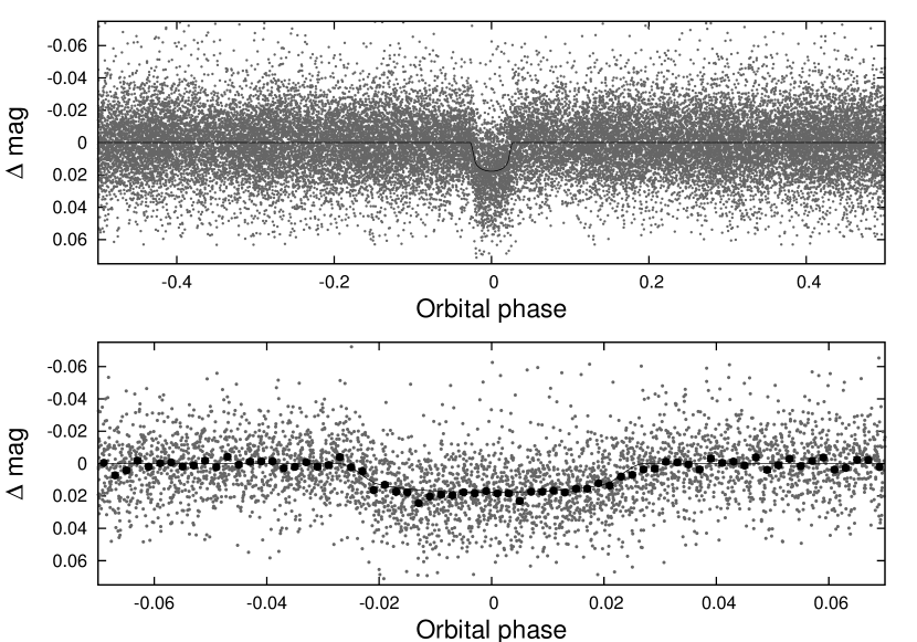
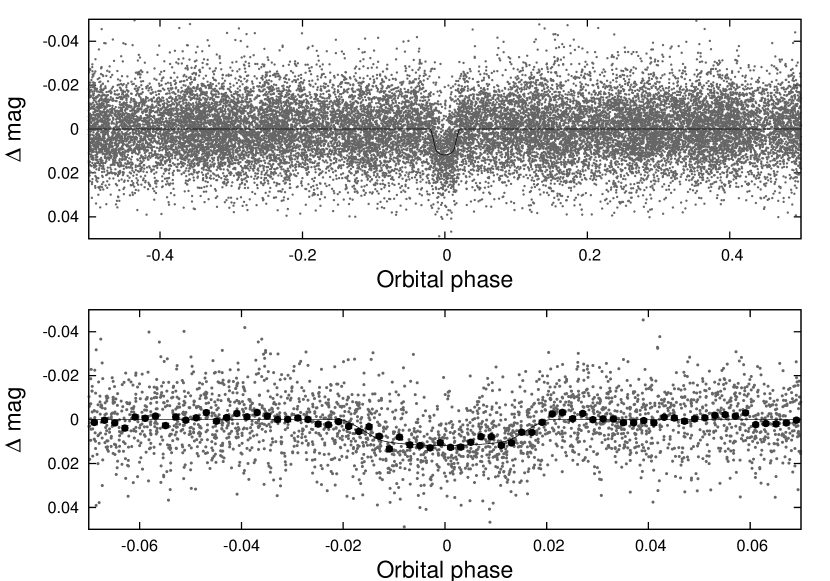
Figure 1.— HATSouth photometry for HATS-15 (left) and HATS-16 (right). The top panel of each system shows the relative full light curve phase-folded and unbinned; the superimposed solid lines are the model fits to the light curves. The bottom panels show the light curve zoomed-in on the transit. The dark filled circles represent the light curves binned in phase with a bin size of 0.002.

Operating since 2010, the HATSouth survey has discovered 16 exoplanets so far, including the two presented in this paper. These planets span a range in masses that goes from super-Neptune (HATS-7 b and HATS-8 b, Bakos et al., 2015; Bayliss et al., 2015) to super-Jupiters (e.g. HATS-11 b and HATS-16 b, Rabus et al., 2015, this work).

The paper is organized as follows: in Section 2 we describe the observations and data reduction that allowed us to discover and confirm the planetary nature of HATS-15b and HATS-16b. In Section 3 we outline the diverse steps of our analysis that brought us to discard the false positive scenarios and determine the stellar and planetary parameters of the two systems. Finally in Section 4, we discuss and summarize our findings.

2. Observations

2.1. Photometric detection

HATS-15 is a $V=14.77$ mag star, located in the Capricornus constellation, while HATS-16 (aka GSC 7516-00867) is a $V=13.83$ mag star in the Sculptor constellation. Both the stars have been identified as planetary host candidates based on roughly six months of continuous photometric observations. Specifically, HATS-15 was in the field-of-view (FOV) of two different HATS-fields (G581 and G582), and was therefore observed from September 2009 to September 2010 with all the units in the three sites. HATS-16 was observed from June 2013 to December 2013 with the HS-2, HS-4 and HS-6 units (located at LCO, HESS and SSO respectively). The target was simultaneously observed with two different cameras in each site, as it was lying in the overlapping region of the FOV of two cameras. Table 1 shows the details of the photometric observations, displaying the total number of photometric measurements, the observing cadence and other information.

The light curves of the two stars were obtained through aperture photometry from the properly calibrated (bias and dark subtracted and flat fielded) science frames following Bakos et al. (2013) and Penev et al. (2013). The light curves were detrended, using the TFA algorithm (Trend Filtering Algorithm; see Kovács et al., 2005), and then searched for a periodical signal by fitting them with a box-shaped transit model (Box Least Square; Kovács et al., 2002). We found that the HATS-15 photometry shows a periodic dip every 1.75 days, while in the HATS-16 light curve we detected a transit signal with a periodicity of 2.69 days. The phase-folded light curves of both the planets are shown in Fig. 1, and the data are provided in Table 2.

Table 1 Summary of photometric observations

Instrument/Field	Date(s)	# Images	Cadence	Filter	Precision
			(sec)		(mmag)
HATS-15
HS-1.3/G581	2009 Aug–2010 Sep	6802	288	$r$	19.1
HS-3.3/G581	2009 Sep–2010 Sep	8617	292	$r$	17.9
HS-5.3/G581	2009 Nov–2010 Sep	586	292	$r$	18.6
HS-2.2/G582	2009 Sep–2010 Sep	4450	284	$r$	19.9
HS-4.2/G582	2009 Sep–2010 Sep	7834	288	$r$	20.0
HS-6.2/G582	2010 Aug–2010 Sep	207	290	$r$	21.7
FTS 2 m/Spectral	2011 Sep 23	87	82	$i$	2.1
PEST 0.3 m	2013 May 21	143	130	$R_{\mathrm{C}}$	12.5
MPG 2.2 m/GROND	2013 Jun 15	71	224	$g$	1.1
MPG 2.2 m/GROND	2013 Jun 15	65	224	$r$	0.8
MPG 2.2 m/GROND	2013 Jun 15	70	224	$i$	1.2
MPG 2.2 m/GROND	2013 Jun 15	72	224	$z$	1.5
HATS-16
HS-2.1/G588	2013 Jun–2013 Oct	3888	279	$r$	12.9
HS-4.1/G588	2013 Jun–2013 Dec	4683	291	$r$	13.5
HS-6.1/G588	2013 Jun–2013 Dec	3618	296	$r$	13.2
HS-2.2/G588	2013 Jun–2013 Oct	1929	281	$r$	12.2
HS-4.2/G588	2013 Jun–2013 Dec	3732	291	$r$	11.9
HS-6.2/G588	2013 Jun–2013 Dec	3678	296	$r$	11.8
DK 1.54 m/DFOSC	2014 Oct 06	170	116	$R$	2.1

Table 2 Light curve data for HATS-15 and HATS-16.

Object	BJD	Mag	$\sigma_{\rm Mag}$	Mag(orig)	Filter	Instrument
	(2,400,000$+$)
HATS-15	$55435.70436$	$-0.02268$	$0.01260$	$\cdots$	$r$	HS
HATS-15	$55374.54242$	$-0.00238$	$0.02157$	$\cdots$	$r$	HS
HATS-15	$55386.77495$	$0.01740$	$0.01000$	$\cdots$	$r$	HS
HATS-15	$55096.69186$	$0.02154$	$0.01436$	$\cdots$	$r$	HS
HATS-15	$55416.48228$	$0.00679$	$0.00988$	$\cdots$	$r$	HS
HATS-15	$55124.65174$	$-0.04501$	$0.01408$	$\cdots$	$r$	HS
HATS-15	$55110.67192$	$-0.00283$	$0.02212$	$\cdots$	$r$	HS
HATS-15	$55367.55285$	$0.02756$	$0.00964$	$\cdots$	$r$	HS
HATS-15	$55381.53294$	$0.00608$	$0.01109$	$\cdots$	$r$	HS
HATS-15	$55409.49282$	$-0.00161$	$0.01282$	$\cdots$	$r$	HS

Note. — This table is available in a machine-readable form in the on-line journal. A portion is shown here for guidance regarding its form and content.

2.2. Spectroscopic Observations

In order to confirm the planetary nature of the two candidates and obtain the complete set of their orbital and physical parameters, systematic spectroscopic observations of the two systems are mandatory. Our observations can be divided in two different steps: first we observed our targets with low resolution spectrographs, or at high resolution but low S/N, to obtain an initial characterization of the star and exclude some of the most probable false positive scenarios; subsequently, we obtained several high-resolution high S/N spectra to measure the radial velocity of the two stars.

Figure 2.— Phased high-precision RV measurements for HATS-15 (left), and HATS-16 (right) from FEROS (filled circles), Coralie (open triangles), and HIRES (open circles). The top panel shows the phased measurements together with our best-fit circular-orbit model (see Table 5) for each system. Zero-phase corresponds to the time of mid-transit and the center-of-mass velocity has been subtracted. The second panel shows the velocity $O\!-\!C$ residuals from the best fit. The error bars include the jitter terms listed in Table 5 added in quadrature to the formal errors for each instrument. The third panel shows the bisector spans (BS). Note the different vertical scales of the panels.

For both the stars we obtained 4 spectra with the Wide-Field Spectrograph (WiFeS) mounted on the 2.3 m ANU telescope located at SSO. WiFeS is an image-slicing integral-field spectrograph (Dopita et al., 2007). According to the different slits used, it can achieve an average resolution up to $R=\lambda/\Delta\lambda\sim$7000 over a wavelength rage of 3300–9200 Å. The spectra were extracted and reduced following Bayliss et al. (2013). One of the spectra, was observed with a resolution of $R=3000$ for obtaining a first spectral classification of each star and verifying that they are not giants. By analyzing the spectra, we found that HATS-15 is a G9 dwarf ($\mathrm{T_{eff,*}}=5000\pm 300$ K and $\log{g_{\star}}=3.5\pm 0.3$) while HATS-16 is a G3 dwarf ($\mathrm{T_{eff,*}}=6300\pm 300$ K and $\log{g_{\star}}=4.6\pm 0.3$). The other three spectra where obtained with a higher resolution ($R=7000$) to look for a possible periodic RV signal higher than 5 km s^-1, which is the signature of an eclipsing binary that is the most probable false positive scenario. In both the cases, we did not find evidence of any RV variation higher than 0.5 km s^-1 for HATS-15 and 2 km s^-1 for HATS-16. Moreover, none of the two systems show a composed spectrum, allowing us to exclude the spectroscopic binary scenario.

Another reconnaissance spectrum for HATS-15 was observed with the du Pont telescope on August 21, 2013. The 2.5 m du Pont telescope is located at LCO, and is equipped with an echelle spectrograph capable to cover the optical range between 3700 and 7000 Å, achieving a maximum resolution of $R\sim$45000. We used a a $1^{\prime\prime}\times 4^{\prime\prime}$ slit that allowed a resolution of $R\sim$40000. The spectrum was reduced with an automated pipeline written for this instrument and similar to the one used for Coralie and FEROS (Brahm et al., 2015).

The reconnaissance spectroscopy observations pointed towards a planetary system scenario for both the systems. Therefore, we started a campaign to get high precision RV measurements, in order to determine the mass of the companions, and verify that the periodical signals in RV were consistent with the photometric ones.

Between June and November 2012 we obtained three high resolution spectra of HATS-15 with Coralie. The spectrograph Coralie is fed from the 1.2 m Swiss-Euler telescope, which is located at the ESO Observatory in La Silla, Chile. The instrument is a fiber-fed spectrograph with a resolution of $R\sim$60000 and a wavelength coverage between 3850 and 6900 Å (Queloz et al., 2001). During each science exposure, a simultaneous ThAr spectra was taken, to be able to operate a proper wavelength calibration. The spectra extraction was performed from the images calibrated with bias and flats obtained during the twilight following Marsh (1989). The RV of each spectrum was then measured by cross-correlation with a binary mask accurately chosen according to the spectral class of the target (for a complete description of the reduction pipeline see Jordán et al., 2014).

The bulk of the RV measurements, which allowed us to verify the planetary nature of both the candidates, was performed by utilizing the Fiber-fed Extended Range Optical Spectrograph (FEROS). It is an echelle spectrograph mounted on the MPG 2.2 m telescope, which is also situated at the La Silla Observatory. The instrument is capable of a wide wavelength coverage from 3700 to 8600 Å and has an average resolution of $R\sim$48000 (Kaufer & Pasquini, 1998). For HATS-15 we observed 13 spectra between September 2011 and May 2013, whereas 12 spectra were obtained for HATS-16 between June and October 2014. The data were reduced and RVs were measured, using the same pipeline written for Coralie and adapted for FEROS (Brahm et al., 2015).

Moreover, we obtained four observations of HATS-16 with HIRES in September 2014. HIRES (HIgh Resolution Echelle Spectrometer) is an echelle spectrograph mounted in the Nasmyth focus of the Keck-I telescope located on the mountain of Mauna Kea in Hawaii, USA. HIRES has a resolution up to 84000 and can cover wavelengths between 3000 and 11000 Å (Vogt et al., 1994). The observations were made using the standard high-precision RV setup for faint targets. We used the C2 decker obtaining a resolution of $R\sim 55000$. Unlike the previous two instruments used for high-resolution spectroscopy, the wavelength calibration was not conducted with the simultaneous observation of a ThAr spectrum, but with an Iodine absorption cell (Marcy & Butler, 1992). The radial velocity extraction was performed using a theoretical synthetic template drawn from the Coelho (2014) grid as described by Fulton et al. (2015). This method provides greater precision measurements for faint stars than the traditional technique of obtaining an additional iodine-free observation to be used as a template (e.g., Bayliss et al., 2015).

The high resolution RV measurements of both the systems showed a periodicity consistent with the one measured form the photometric observations. A periodic signal, presented both in the light curve and in the RV, might not be necessarily due to the presence of a planetary companion, but can be produced by a blended eclipsing binary. To exclude this false positive scenario we measured the bisector span (BS) for both the systems finding no hint of a periodicity consistent with the orbital period; for the BS measurements we followed a procedure similar to that of Torres et al. (2007), appropriately adapted to each instrument. The spectroscopic observations are summarized in Table 3, and phased high-precision RV and BS measurements are shown for each system in Figure 2.

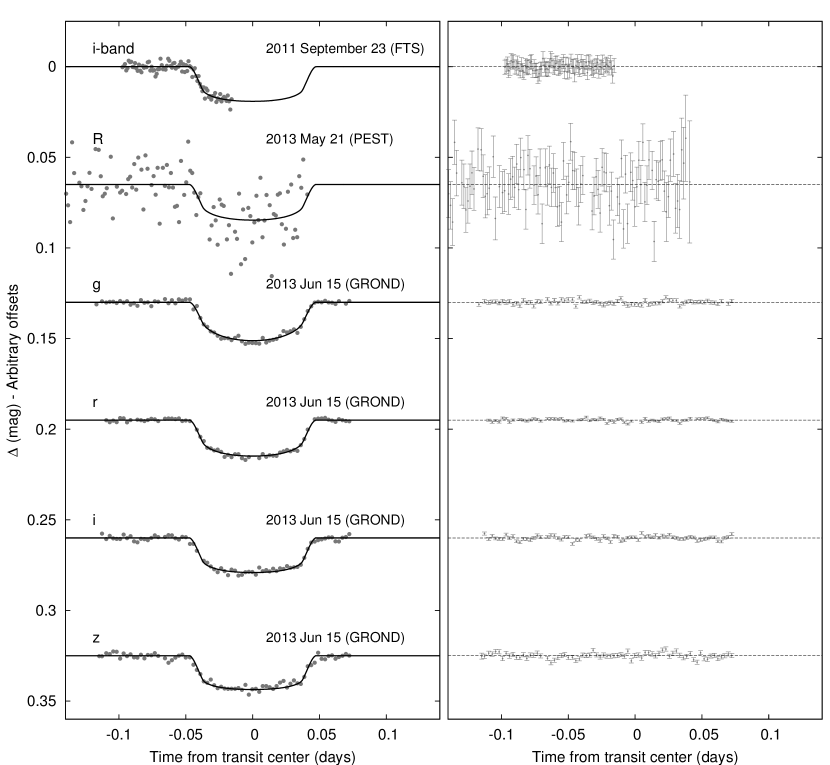
Figure 3.— Left: Unbinned transit light curves for HATS-15. The light curves have been corrected for quadratic trends in time fitted simultaneously with the transit model. The dates of the events, filters and instruments used are indicated. Light curves following the first are displaced vertically for clarity. Our best fit from the global modeling described in Section 3.5 is shown by the solid lines. Right: residuals from the fits are displayed in the same order as the left curves. The error bars represent the photon and background shot noise, plus the readout noise.

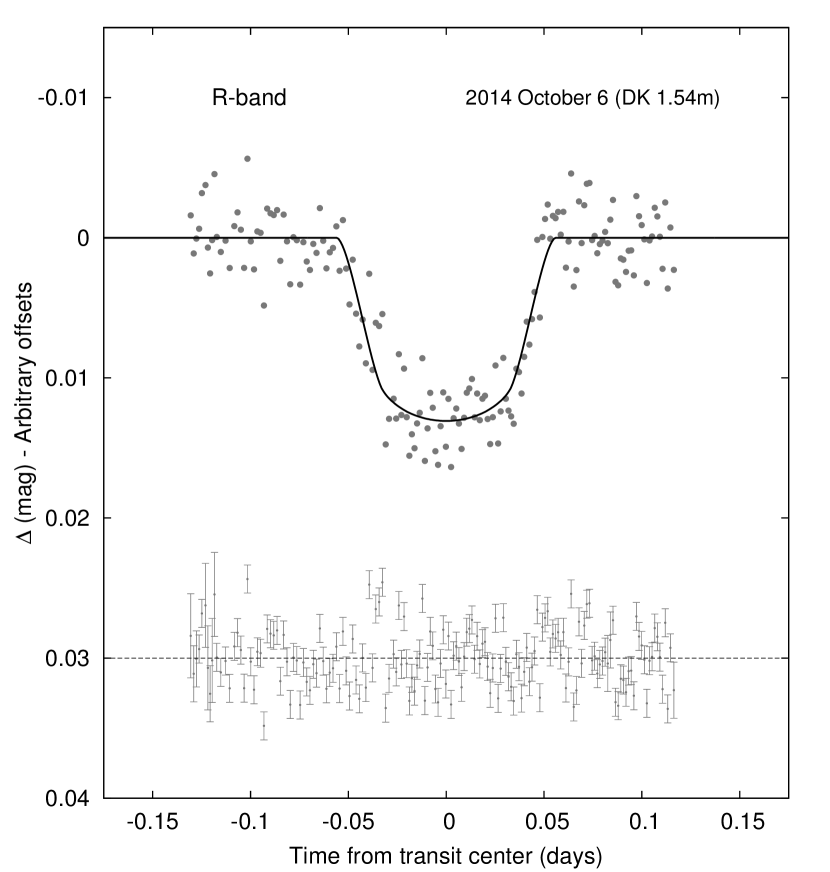
Figure 4.— Similar to Figure 3; we show the follow-up light curve for HATS-16. In this case, variations in the light curve that are correlated with the FWHM of the PSF are corrected simultaneously to the fitting of the transit.

Finally, four further high–resolution spectra of HATS-15 were obtained in August-September 2014 with the Planet Finder Spectrograph (PFS). PFS is an echelle spectrograph mounted on the 6.5 m Magellan Clay Telescope at Las Campanas Observatory in Chile. The maximum wavelength coverage PSF is capable of span the optical region from 3880 to 6680 Å, and can be used in different modes, yielding a maximum resolution of $R\sim 190000$ (Crane et al., 2010). For our observations, we used a $0.5^{\prime\prime}\times 2.5^{\prime\prime}$ slit having a resolving power of 76000. These spectra were used to determine the spectroscopic parameters for HATS-15 using the ZASPE program (see Section 3), while for HATS-16 the parameters have been measured by applying the same program to a combination of the FEROS spectra.

Table 3 Summary of spectroscopy observations

Instrument	UT Date(s)	# Spec.	Res.	S/N Range	$\gamma_{\rm RV}$	RV Precision
			$\Delta\lambda$/$\lambda$/1000		($\mathrm{km\,s}^{-1}$)	($\mathrm{m\,s}^{-1}$)
HATS-15
Reconnaissance
ANU 2.3 m/WiFeS	2011 Jul 26–28	3	7	13–22	-54.7	4000
ANU 2.3 m/WiFeS	2011 Jul 27	1	3	95	$\cdots$	$\cdots$
du Pont 2.5 m/Echelle	2013 Aug 21	1	40	36	-53.8	500
High resolution radial velocity
MPG 2.2 m/FEROS	2011 Sep–2013 May	13	48	16–49	-54.145	81
Euler 1.2 m/Coralie	2012 Jun–Nov	3	60	12–13	-54.270	246
Magellan 6.5 m/PFS	2014 Sep	4	76	40	$\cdots$	$\cdots$
HATS-16
Reconnaissance
ANU 2.3 m/WiFeS	2014 Jun 3–5	3	7	21–82	28.7	4000
ANU 2.3 m/WiFeS	2014 Jun 4	1	3	101	$\cdots$	$\cdots$
Euler 1.2 m/Coralie	2014 Jun 20	1	60	14	31.625	100
High resolution radial velocity
MPG 2.2 m/FEROS	2014 Jun–Oct	12	48	35–57	31.594	54
Keck 10 m/HIRES	2014 Jun 20	4	55	$\cdots$	$\cdots$	20

2.3. Photometric follow-up observations

Both the HATS-15 and HATS-16 planetary systems have been photometrically followed-up to properly constrain their orbital ephemeris and obtain a precise measure of the photometric parameters, which allow to directly estimate the mean density of the parent stars and, at the end, the radii of the planets. The photometric follow-up observations are summarized in Table 1 and the corresponding data are reported in Table 2 for both the systems.

We observed two partial transits and a complete one of HATS-15. Specifically, the first half transit was obtained with the Faulkes Telescope South (FTS) on September the $23^{\mathrm{th}}$ 2011, and consisted in the out-of-transit data, ingress and partial transit observation. The FTS is a 2.0 m telescope, located at SSO, and is part of the Las Cumbres Observatory Global Telescope (LCOGT) network. The telescope is equipped with a $4000\times 4000$ pixels camera with a pixel size of 0.15^′′. The observations were performed with an i-band filter and with the telescope out of focus, as no close-in background star was detected. The data reduction was performed using an automated aperture photometry pipeline utilising Sextractor (Bertin & Arnouts, 1996). In brief the science images are first calibrated via bias subtraction and flat-fielding, then the light curves are extracted via fix-aperture photometry.

The second-half transit was observed with the 30 cm PEST telescope on May the $21^{\mathrm{st}}$ 2013, and covered almost the whole transit excluding egress. The SBIG ST-8XME camera mounted on this telescope has a FOV of $31^{\prime}\times 21^{\prime}$, with a resolution of 1.2 arcsec per pixel. A $R_{\mathrm{C}}$ filter was used to take in-focus images with a cadence of 130 s. The light curve was extracted from the calibrated images (dark subtracted and flat-fielded) with aperture photometry. For a more exhaustive overview on the instrument’s characteristics and the data reduction description see Zhou et al. (2014).

A complete transit of HATS-15b was observed simultaneously in four different optical bands ($g^{\prime}$, $r^{\prime}$, $i^{\prime}$, $z^{\prime}$, similar to Sloan filters) using the multiband imager instrument GROND (Gamma Ray Optical Near-infrared Detector; Greiner et al., 2008). The observations, performed on June the $15^{\mathrm{th}}$ 2013, were obtained with the telescope slightly out of focus to increase the photometric precision. After de-biasing and flat-fielding the science frames, the photometry was extracted with a pipeline based on DAOPHOT that make use of the APER IDL function (for the GROND observing strategy and subsequent data reduction refer to Penev et al., 2013; Mohler-Fischer et al., 2013). The light curves for all the HATS-15 follow-up transits are shown in Figure 3.

We obtained a transit of HATS-16 with the DFOSC camera on October the $6^{\mathrm{th}}$ 2014. The DFOSC (Danish Faint Object Spectrograph and Camera) instrument is mounted on the 1.54 m Danish Telescope, at the La Silla Observatory. The CCD has a resolution of 0.39 arcsec per pixel and a FOV $13.7^{\prime}\times 13.7^{\prime}$. The telescope was defocused and a Bessel $R$ filter was used. After properly calibrating the images, aperture photometry was done following Deeg & Doyle (2001) to obtain the light curve. See Rabus et al. (2015) for a complete description of the instrument and reduction pipeline. The light curve for HATS-16 is shown in Figure 4.

Table 4 Stellar parameters for HATS-15 and HATS-16

	HATS-15	HATS-16
Parameter	Value	Value	Source
Astrometric properties and cross-identifications
2MASS-ID	2MASS 20442207-1926150	2MASS 23541409-3000467
GSC-ID	—	GSC 7516-00867
R.A. (J2000)	$20^{\mathrm{h}}44^{\mathrm{m}}22.20^{\mathrm{s}}$	$23^{\mathrm{h}}54^{\mathrm{m}}14.04^{\mathrm{s}}$	2MASS
Dec. (J2000)	$-19{\arcdeg}26{\arcmin}15.0{\arcsec}$	$-30{\arcdeg}00{\arcmin}46.8{\arcsec}$	2MASS
$\mu_{\rm R.A.}$ ($\rm mas\,yr^{-1}$)	$19.6\pm 2.5$	$21.7\pm 1.3$	UCAC4
$\mu_{\rm Dec.}$ ($\rm mas\,yr^{-1}$)	$3.7\pm 2.4$	$-2.6\pm 1.2$	UCAC4
Spectroscopic properties
$T_{\rm eff\star}$ (K)	$5311\pm 77$	$5738\pm 79$	ZASPE
$\rm[Fe/H]$	$0.000\pm 0.050$	$−0.100\pm 0.050$	ZASPE
$v\sin{i}$ ($\mathrm{km\,s}^{-1}$)	$4.18\pm 0.50$	$6.17\pm 0.22$	ZASPE
$v_{\rm mac}$ ($\mathrm{km\,s}^{-1}$)	3.3	4.0	Assumed
$v_{\rm mic}$ ($\mathrm{m\,s}^{-1}$)	0.85	1.06	Assumed
$\gamma_{\rm RV}$ ($\mathrm{km\,s}^{-1}$)	$−54.145\pm 0.020$	$31.594\pm 0.023$	FEROS
Photometric properties
$B$ (mag)	$15.797\pm 0.030$	$14.477\pm 0.060$	APASS
$V$ (mag)	$14.774\pm 0.010$	$13.834\pm 0.020$	APASS
$g$ (mag)	$15.323\pm 0.010$	$14.086\pm 0.020$	APASS
$r$ (mag)	$14.592\pm 0.010$	$13.645\pm 0.010$	APASS
$i$ (mag)	$14.320\pm 0.010$	$13.496\pm 0.030$	APASS
$J$ (mag)	$13.261\pm 0.027$	$12.652\pm 0.024$	2MASS
$H$ (mag)	$12.806\pm 0.024$	$12.335\pm 0.025$	2MASS
$K_{s}$ (mag)	$12.724\pm 0.032$	$12.280\pm 0.021$	2MASS
Derived properties
$M_{\star}$ ($M_{\sun}$)	$0.871\pm 0.023$	$0.970\pm 0.035$	YY+$\rho_{\star}$+ZASPE
$R_{\star}$ ($R_{\sun}$)	$0.922\pm 0.027$	$1.238^{+0.097}_{−0.127}$	YY+$\rho_{\star}$+ZASPE
$\log{g_{\star}}$ (cgs)	$4.449\pm 0.022$	$4.239\pm 0.079$	YY+$\rho_{\star}$+ZASPE
$\rho_{\star}$ ($\rm g\,cm^{-3}$)	$1.57\pm 0.12$	$0.72^{+0.26}_{−0.13}$	YY+$\rho_{\star}$+ZASPE
$L_{\star}$ ($L_{\sun}$)	$0.625\pm 0.057$	$\pm$	YY+$\rho_{\star}$+ZASPE
$M_{V}$ (mag)	$5.43\pm 0.11$	$\pm$	YY+$\rho_{\star}$+ZASPE
$M_{K}$ (mag,ESO)	$3.556\pm 0.071$	$\pm$	YY+$\rho_{\star}$+ZASPE
Age (Gyr)	$11.0^{+1.4}_{−2.0}$	$9.5\pm 1.8$	YY+$\rho_{\star}$+ZASPE
$A_{V}$ (mag)	$0.151\pm 0.063$	$0.000\pm 0.021$	YY+$\rho_{\star}$+ZASPE
Distance (pc)	$689\pm 23$	$774\pm 74$	YY+$\rho_{\star}$+ZASPE
$P_{\mathrm{rot\star}}$ (d)	$\cdots$	$12.350\pm 0.024$	HATS light curves

Note. — For HATS-15 b the fixed-circular-orbit model has a Bayesian evidence that is $\sim 2$ times larger than the evidence for the eccentric-orbit model, while for HATS-16 b the fixed-circular-orbit model has a Bayesian evidence that is $\sim 6$ times larger than the evidence for the eccentric-orbit model. We therefore assume a fixed circular orbit in generating the parameters listed here.

3. Analysis

3.1. Properties of the parent star

For achieving a precise determination of the physical properties of a new exoplanet, it is crucial to properly characterize its host star, especially its mass and radius. We obtained those quantities, and the other set of parameters describing the HATS-15 and HATS-16 stars, by properly combining the spectroscopic and photometric data.

The atmospheric parameters, including the effective temperature $T_{\mathrm{eff}}$, surface gravity $\log{g}$, metallicity [Fe/H] and the projected rotational velocity $v\sin{i}$, were measured by analyzing the high resolution spectra obtained with PFS for HATS-15 and FEROS for HATS-16. The analysis was performed using the Zonal Atmospherical Stellar Parameter Estimator (ZASPE) code (see Brahm et al., 2015). In brief, the atmospheric parameters are calculated iteratively, selecting a specific region of the spectra (between 5000 Å and 6000 Å) and fitting the median-combined observed spectra with a grid of synthetic ones (Husser et al., 2013). For HATS-15 we found: $T_{\mathrm{eff}}=5296\pm 76$, $\log{g}=4.60\pm 0.12$, [Fe/H]=$0.090\pm 0.040$ and $v\sin{i}=4.36\pm 0.24$; while for HATS-16: $T_{\mathrm{eff}}=5840\pm 120$, $\log{g}=4.50\pm 0.19$, [Fe/H]=$−0.010\pm 0.070$ and $v\sin{i}=6.01\pm 0.50$.

The fundamental stellar parameters were obtained combining the spectroscopic and photometric quantities with the Yonsei-Yale stellar evolutionary models (Y2 hereafter; Yi et al., 2001). In particular, for the analysis with the isochrones, we used the stellar density $\rho_{\star}$ obtained from the photometry instead of $\log{g}$ from the spectra, as it provides a more precise and more accurate constraint on the stellar properties (following Sozzetti et al., 2007). Assuming a nil eccentricity of the planetary orbit, the stellar density can be directly measured from the transit light curve as described in Seager & Mallén-Ornelas (2003).

For both the systems we performed a second time the analysis: first we re-derived the spectroscopic quantities with ZASPE, this time fixing the values of the log g to the ones retrieved from the stellar evolution models. Then we obtained the stellar properties once more modeling the data with the Y2 isochrones. We found that HATS-15 has a mass $M_{\star}=0.871\pm 0.023\,M_{\sun}$, radius $R_{\star}=0.922\pm 0.027\,R_{\sun}$ and an age of $11.0^{+1.4}_{-2.0}$ Gyr; while HATS-16 has $M_{\star}=0.970\pm 0.035\,M_{\sun}$, $R_{\star}=1.238^{+0.097}_{-0.127}\,R_{\sun}$ and age=$9.5\pm 1.8$ Gyr. The final values adopted in the subsequent analysis to derive the planetary parameters are presented in Table 4, while in Figure 5 the two stars are shown in a $T_{\rm eff\star}$–$\rho_{\star}$ diagram (similar to a Hertzsprung-Russell diagram).

To measure the distance of the two planetary systems we compared the magnitude observed with each filter with a set of predicted ones. The predicted magnitudes were determined using the Y2 isochrones and assuming an extinction law with $R_{\mathrm{V}}=3.1$ from Cardelli et al. (1989). Using the NASA/IPAC Extragalactic Database (NED) we checked that the value for the extinction were consistent with the expected reddening at the Galactic position of both the systems. We found that, within the error bars the $A_{\mathrm{V}}$ are consistent with those predicted from the extinction map by Schlegel et al. (1998) and Schlafly & Finkbeiner (2011). HATS-15 is $690\pm 23$ pc distant from the Sun, and HATS-16 is slightly farther away at $774\pm 74$ pc.

Figure 5.— Model isochrones from Yi et al. (2001) for the measured metallicities of HATS-15 (left) and HATS-16 (right). We show models for ages of 0.2 Gyr and 1.0 to 14.0 Gyr in 1.0 Gyr increments (ages increasing from left to right). The adopted values of $T_{\rm eff\star}$ and $\rho_{\star}$ are shown together with their 1$\sigma$ and 2$\sigma$ confidence ellipsoids. The initial values of $T_{\rm eff\star}$ and $\rho_{\star}$ from the first ZASPE and light curve analysis are represented with a triangle.

Table 5Orbital and planetary parameters for HATS-15 b and HATS-16 b

	HATS-15 b	HATS-16 b
Parameter	Value	Value
Light curve parameters
$P$ (days)	$1.74748753\pm 0.00000094$	$2.686502\pm 0.000011$
$T_{c}$ (${\rm BJD}$)	$2456387.21161\pm 0.00015$	$2456824.79069\pm 0.00076$
$T_{12}$ (days)	$0.09457\pm 0.00074$	$0.1092v0.0032$
$T_{12}=T_{34}$ (days)	$0.01144\pm 0.00069$	$0.0211\pm 0.0044$
$a/R_{\star}$	$6.33\pm 0.16$	$6.50^{+0.70}_{−0.43}$
$\zeta/R_{\star}$	$23.991^{+0.118}_{−0.081}$	$22.27\pm 0.49$
$R_{p}/R_{\star}$	$0.1229\pm 0.0012$	$0.1075\pm 0.0037$
$b^{2}$	$0.100^{+0.044}_{−0.054}$	$0.536^{+0.065}_{−0.125}$
$b\equiv a\cos i/R_{\star}$	$0.317^{+0.064}_{−0.101}$	$0.732^{+0.043}_{−0.091}$
$i$ (deg)	$87.13^{+0.97}_{−0.67}$	$83.53^{+1.37}_{−0.86}$0
Limb-darkening coefficients
$c_{1},g$ (linear term)	0.6795	$\cdots$
$c_{2},g$ (quadratic term)	0.1376	$\cdots$
$c_{1},r$	0.4560	0.3526
$c_{2},r$	0.2619	0.3264
$c_{1},i$	0.3470	$\cdots$
$c_{2},i$	0.2834	$\cdots$
$c_{1},z$	0.2742	$\cdots$
$c_{2},z$	0.2937	$\cdots$
$c_{1},R$	0.4259	0.3289
$c_{2},R$	0.2687	0.3276
RV parameters
$K$ ($\mathrm{m\,s}^{-1}$)	$399\pm 26$	$485\pm 25$00
$e$	$<0.126$	$<0.000$
Planetary parameters
$M_{p}$ ($M_{\rm J}$)	$2.17\pm 0.15$	$3.27\pm 0.19$
$R_{p}$ ($R_{\rm J}$)	$1.105\pm 0.040$	$1.30\pm 0.15$
$C(M_{p},R_{p})$	$0.18$	$0.10$
$\rho_{p}$ ($\rm g\,cm^{-3}$)	$1.97\pm 0.24$	$1.86^{+0.94}_{−0.48}$
$\log g_{p}$ (cgs)	$3.641\pm 0.040$	$3.685^{+0.117}_{−0.086}$
$a$ (AU)	$0.02712\pm 0.00023$	$0.03744\pm 0.00045$
$T_{\rm eq}$ (K)	$1505\pm 30$	$1592^{+61}_{−82}$
$\Theta$	$0.1211\pm 0.0088$	$0.194^{+0.030}_{−0.021}$
$\log_{10}\langle F\rangle$ (cgs)	$9.064\pm 0.035$	$9.161^{+0.065}_{−0.092}$

Note. — For HATS-15 b the fixed-circular-orbit model has a Bayesian evidence that is $\sim 2$ times larger than the evidence for the eccentric-orbit model, while for HATS-16 b the fixed-circular-orbit model has a Bayesian evidence that is $\sim 6$ times larger than the evidence for the eccentric-orbit model. We therefore assume a fixed-circular-orbit in generating the parameters listed here.

3.2. Rotational modulation

We inspected the entire light curves obtained from the HATS survey of both HATS-15 and HATS-16, in order to look for possible periodic modulations, caused by the presence of star spots on the surface of the host stars.

Already with a quick look at the light curves, it is possible to identify a periodicity around 12-13 days for HATS-16, while no perceivable modulation is visible in the HATS-15 photometry. In order to quantify the variability and check for possible false alarm, we used GLS, a FORTRAN based routine by Zechmeister & Kürster (2009), to calculate the generalized Lomb-Scargle periodogram. In brief the data are fitted with a sinusoidal function at different frequencies starting from a provided minimum of 0.0056 [1/d] (that is related to the time range over which the photometric data were acquired) to a maximum frequency of 22.33, with about 79000 steps. A window function is also provided, giving information on the possible false periodicity created by the data sampling. We found a peak in the frequencies corresponding to a period of $P=12.350\pm 0.024$ days and an amplitude of $2.91\pm 0.47$ mmag, with an extremely low false alarm probability (FAP, Cumming, 2004).

As a sanity check, we obtained the periodogram in several different ways always obtaining consistent values of the period. In particular, we calculated the periodogram both for the un-binned and binned data (using several bin sizes) and using also another program (Systemic2, by Meschiari et al., 2009) besides GLS. If the modulation is due to the activity of the star, then the amplitude of the periodic signal may vary in time with the spot coverage, while the period remains constant. We checked for this effect by dividing our data-set into three segments and calculating a periodogram for each one. The three periods are consistent within the error bars, even if in the last dataset the significance of the first peak is lower, as the amplitude of the signal is smaller than that in the first two cases. We assume the variability is due to the apparent spot coverage of the star changing as the star rotates and take the photometric period to be a measure of the stellar rotational period.

By comparing the rotational period found from the photometry to that inferred from the spectroscopic $v\sin i$ (assuming $\sin i=1$ and propagating the errors we obtain $P=10.148^{+0.874}_{-1.102}$ days), we find a slight inconsistency: the two periods are nearly $2\sigma$ away, and the latter is smaller than the first one. However, we stress that the measurement of the $v\sin{i}$ should be considered as an upper limit. It actually describes the broadening of the spectral lines that is caused by a multiplicity of other effects, which are difficult to take into account. Moreover, the rotational period found from photometry doesn’t take into account the possibility to have differential rotation. As the latitude of the spot group causing the photometric signal is unknown, the mean period might be larger (if the spots lie around the equator) or smaller (if the spots have a high latitude).

The periodogram, and the phase folded HATSouth photometry with the period of $P=12.35$ d are shown in Figure 6.

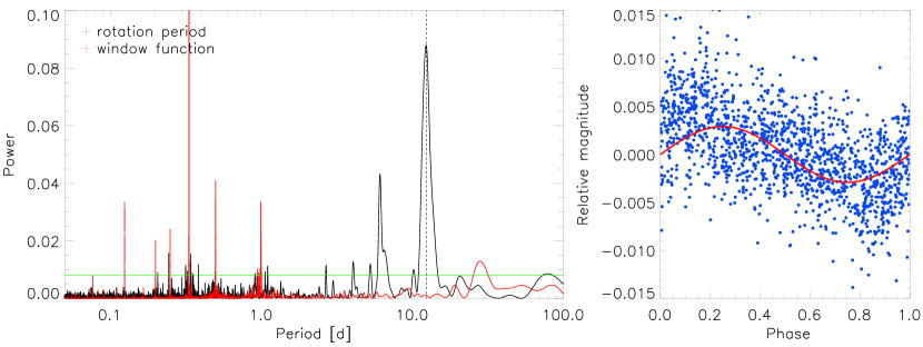
Figure 6.— Left: periodogram for the HATSouth photometric data of HATS-16 obtained during the $\sim$6 months of observations. The horizontal green line represent the false alarm probability FAP= 0.0001, wile the vertical dashed line corresponds to the maximum probability peak. In the same panel the window function is displayed with red lines. Right: HATSouth photometric data phase folded and binned in 0.001 phase bins for the period (P=12.35 d). The red solid line represents the best sinusoid fit with period fixed to the one found from the periodogram and an amplitude of $\sim$ 2.9 mmag.

3.3. Age of the systems

To determine the age of the two planetary systems, we used different methods. A first determination for both the systems was done by modeling the stellar parameters with the Y2 evolutionary model, which was already used in 3.1. We found an age of $11.0^{+1.4}_{-2.0}$ Gyr and $9.5\pm 1.8$ Gyr for HATS-15 and HATS-16, respectively, which suggest that both the systems are old with respect to the average ages of stars in similar spectral class and of exoplanets host in general (e.g. Bonfanti et al., 2015).

Since the rotation of a star is expected to slow down during its lifetime (e.g. Soderblom, 1983), it is therefore possible to correlate the stellar period to its age through the gyrochronology. According to Barnes (2007) the errors in the age estimation via gyrochronology for G and K stars are about 28%. Following the relations in Barnes (2007), and using the improved coefficients values from Angus et al. (2015), we calculated the gyrochronology age of HATS-16 from the rotational period, finding that is younger than 1 Gyr. Using gyrochronology we also calculated the lower limit for the age of HATS-15 using the period obtained from $v\sin i$ and assuming $i=90\deg$. However the lower limit we found of $\gtrsim 0.5$ Gyr does not give any useful constraint.

As expected from the rotational modulation (Figure 6), the HATS-16 star is slightly active and shows a cromospheric emission in the core of the Ca H & K absorption lines. We quantified this activity by calculating the activity indices from the ratio of the emission in the line cores, obtaining $S=0.2524$ and $\log{R^{\prime}_{\mathrm{H\,K}}}=-4.644$. Then, using the age-activity relation presented in Mamajek & Hillenbrand (2008), we estimated that the expected age of the star is 1.47 Gyr, compatible with the age based on gyrochronology, but substantially younger than the isochrone-based age.

A further way to constrain the age of a star is to measure its peculiar velocity in the Galactic frame and compare it with those of other stars in our Galaxy, whose age are well determined. Knowing the position of the planetary systems and their kinematics (radial velocity and proper motion measurements from Table 4), one may convert them to peculiar velocities $U$, $V$, $W$ that describe the motion of a star in galactic coordinates. Specifically, $U$ represents the radial component of the velocity, $V$ is the circular component, and $W$ is the vertical component with respect to the Milky Way disk. To compute the peculiar velocity of HATS-15 and HATS-16, we used a web-based calculator provided by D. Rodriguez. We then corrected our velocity values for the peculiar motion of the Sun ($U_{\sun}=7.01\pm 0.20$ km s^-1, $V_{\sun}=10.13\pm 0.12$ km s^-1 and $W_{\sun}=4.95\pm 0.09$ km s^-1, Huang et al., 2015). The results obtained for both the planets are $U=-75.89$ km s^-1, $V=6.18$ km s^-1 and $W=-12.03$ km s^-1 for HATS-15 and $U=-41.72$ km s^-1, $V=-30.85$ km s^-1 and $W=-43.00$ km s^-1 for HATS-16. For a very young star on a circular orbit, $U$ and $W$ should be close to 0 km s^-1; stars with ages around 1 Gyr can have a higher dispersion in velocities, with an average value of the order of $10-12$ km s^-1; finally, at an age around 10 Gyr, the velocities are expected to be of the order of $25-35$ km s^-1 (Binney et al., 2000). This increase in velocity dispersion with age can be explained taking into account the fact that stars, initially formed in the galactic plane (where molecular clouds and star forming region are mainly located), interact with the galactic environment and gain vertical and radial velocity component in the galactic reference frame (Nordström et al., 2004, and reference therein). The peculiar velocities of our two stars, compared with the average velocities for the stars in our Galaxy, point towards an old age, which is in good agreement with the ones that we found from the isochrone fitting.

3.4. Excluding blend scenarios

One of the most common false positive scenarios for candidates produced by transiting surveys are blends. We attempt to exclude the possibility that our two planetary systems are not hosting planets, but instead are diluted eclipsing binaries, following Hartman et al. (2012).

We modeled the available photometric data for each object as a blend between an eclipsing binary star system and a third star along the line of sight. The physical properties of the stars were constrained using the Padova isochrones (Bertelli et al., 2008), while we also required that the brightest of the three stars in the blend had atmospheric parameters consistent with those measured with ZASPE.

We found that for both HATS-15 and HATS-16, a model consisting of a single star with a transiting planet provides a lower $\chi^{2}$ fit to the available photometric data than any of the blended stellar eclipsing binary models tested. Based solely on the photometry, for HATS-15 we ruled out blend models with $\sim 1\sigma$ confidence, while for HATS-16 we rule them out with $\sim 2\sigma$ confidence. Moreover, we found that for both systems any blend model that could plausibly fit the photometry (i.e., which cannot be rejected with greater than $5\sigma$ confidence) would have been easily identified as a composite system based on the spectroscopic observations. Indeed, we simulated the cross-correlation functions for these possible blend systems, finding that in all the cases, at some of the observed phases, a double peak should have been seen, and that all of the blend scenarios which could plausibly fit the photometry of either system would have produced large RV and BS variations (greater than 1 $\mathrm{km\,s}^{-1}$), which is in conflict with the observations. We conclude, therefore, that both HATS-15 and HATS-16 are transiting planet systems, and that neither object is a blended stellar eclipsing binary system.

Albeit we can rule out the possibility that the two systems are not blended by an eclipsing binary, we cannot rule out the possibility that one of the two systems is a transiting planet system, whose photometry is diluted by the light coming from an unresolved stellar component. For HATS-15 we find that a system consisting of a $0.84\,M_{\sun}$ star with a transiting planet and a $0.65$ $M_{\sun}$ binary companion provides a slightly better fit to the photometric data ($\sim 1.5\sigma$) than the best-fit single-star-with-planet model. The secondary-to-primary $V$-band light ratio of this binary system is 14%, which would be marginally detectable in the observed CCFs unless the system were near conjunction. We also find that a binary star companion of any mass, up to that of the transiting planet host, provides a fit to the photometric data which cannot be distinguished from the best-fit single-star-with-planet model. For HATS-16 we find that binary star systems with a secondary mass between $0.65\,M_{\sun}$ and $0.8\,M_{\sun}$ can be ruled out at $3\sigma$ confidence based on the photometry. This is driven by the broad-band photometric colors which are consistent with the measured effective temperature of the primary star assuming no reddening. Binary companions close in mass to the primary yield similar photometric colors and are not ruled out, while binary companions below $0.65$ $M_{\sun}$ are too faint to significantly affect the photometric colors. Higher spatial resolution imaging and/or continued RV monitoring would be needed to search for binary star companions to either system. For the remainder of the paper we assume that each of the two systems is an isolated star with a close-in transiting planet.

3.5. Global modeling of the data

In order to measure the physical properties of the two planets, we modeled all the photometric and spectroscopic data in our possession following the same approach as in Pál et al. (2008); Bakos et al. (2010); Hartman et al. (2012).

As far as it concerns the light curves, both the HATSouth and the follow-up ones, the fit was performed using the transit models from Mandel & Agol (2002), employing a quadratic law to describe the limb darkening effect, and fixing the coefficients to those from Claret (2004). In the case of the HATSouth photometry, in modelling the transit depth, we included an extra parameter describing the possible dilution caused by the blending of neighboring stars, and the over-correction by the trend-filtering method. To correct for systematic errors in the photometry of the follow-up light curves, a quadratic trend was included in the model of each transit event. The RV data were fitted with Keplerian orbits, allowing the zero-point and the RV jitter for each instrument to vary independently as a free parameter.

To determine the posterior distribution of the parameters and obtain the relative uncertainties we used a Differential Evolution Markov Chain Monte Carlo (DEMCMC ter Braak, 2006; Eastman et al., 2013).

We fitted both fixed circular orbits and free-eccentricity models to the data, and for both systems found that the data are consistent with a circular orbit. As for both systems the fixed circular orbit model had a higher Bayesian evidence, we adopted the parameters assuming no eccentricity for either object.

The parameters obtained from this analysis for each system are listed in Table 5. In brief we found that HATS-15b has a mass of $M=2.17\pm 0.15\,M_{\mathrm{J}}$ and a radius of $R=1.105\pm 0.040\,R_{\mathrm{J}}$, resulting in a bulk density of $\rho=1.48\pm 0.18\,\rho_{\mathrm{J}}$. For HATS-16b, we found that it is more massive, $M=3.27\pm 0.19\,M_{\mathrm{J}}$, and larger, $R=1.30\pm 0.15\,R_{\mathrm{J}}$, which imply a slightly lower density, $\rho=1.39_{-36}^{+0.71}\,\rho_{\mathrm{J}}$.

4. Discussion and Conclusion

We have presented the discovery of HATS-15b and HATS-16b, two massive hot Jupiters orbiting around old dwarf stars. By carefully analyzing the photometric and spectroscopic data, we can exclude false positive scenarios, confirming the planetary nature of the transiting bodies. We found that HATS-15 is a planetary system, $\sim 690$ pc far away from our Sun, that hosts a $2.17\pm 0.15\,M_{\mathrm{J}}$ hot Jupiter, which orbits around a G9 V star in $\sim 1.75$ days. HATS-16b is a massive $3.27\pm 0.19\,M_{\mathrm{J}}$ hot Jupiter $\sim 770$ pc away from us, and is orbiting a G3 V star in $\sim 2.69$ days. Fig. 7 shows the locations of the two new planets in the period–mass diagram, together with the other known transiting exoplanets.

In § 3.3, we have presented several methods to estimate the stellar ages. In the case of HATS-15, the two different methods that we used (Y2 isochrones fitting and stellar kinematics) gave consistent values; we therefore adopted the value found from the modeling with the Y2, which dates the star to be $11.0^{+1.4}_{-2.0}$ Gyr old.

Concerning HATS-16, instead, we found a strong discrepancy between the age measured with Y2 and stellar kinematics, compared with the one obtained with gyrochronology and stellar activity. However, we believe that the age obtained from the stellar evolutionary models ($9.5\pm 1.8$ Gyr) is more reliable than the very young age found based on its activity. Indeed, an old age is more compatible with the slightly low density of the star, compared to what is expected for a young star with its effective temperature and metallicity. By studying all the exoplanetary host stars for which the rotational period is measured, Maxted et al. (2015) found that there is no evidence for the gyrochronological ages to be on average smaller than those measured from isochronal models. Therefore the cause of the discrepancy seen in our measurements has to be searched elsewhere, and not in a measurement bias. The short rotation period (12.4 d) of HATS-16, may be explained in a planet-star interaction context, in which the star has been tidally spun up by the planet (e.g. Pont, 2009; Husnoo et al., 2012). Given the mass of the planet, its distance from the star, and assuming a stellar tidal quality factor (i.e. the efficiency of tidal dissipation in the star) $Q_{*}$=10⁶, obtained from a rough estimation of the orbital evolution timescale (following Penev & Sasselov, 2011), we calculated that just few Gyr are necessary for spinning up the star to its current rotation (here we have assumed that all the angular momentum is dumped in the convective zone, and that only a few percent change in the orbital period is needed).

Considering the entire population of known gas planets, most of the planets in the high-mass regime are found to orbit their star at a large distance, and just few tens are hot Jupiters (see Fig. 7). The rareness of massive giants with $M\gtrsim 2\,M_{\mathrm{J}}$ and $P\lesssim 5$ d cannot be explained by observational biases, since the two more efficient detection methods (transit and RV) are more prone to find massive planets in short orbits than in larger ones

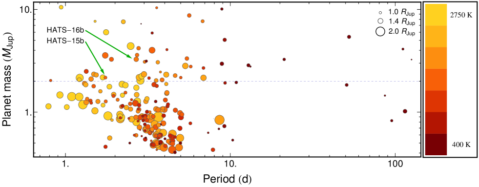
Figure 7.— Mass–period diagram of transiting exoplanets in the mass range $0.4\,M_{\mathrm{J}}<M_{\mathrm{p}}<10\,M_{\mathrm{J}}$. The planets are represented by circles, whose size is proportional to planet radius. Color indicates equilibrium temperature. The dashed line demarcates the high-mass regime ($M_{\mathrm{p}}>2\,M_{\mathrm{J}}$). The error bars have been suppressed for clarity. Data taken from the Transiting Extrasolar Planet Catalogue (TEPCat), which is available at http://www.astro.keele.ac.uk/jkt/tepcat/.

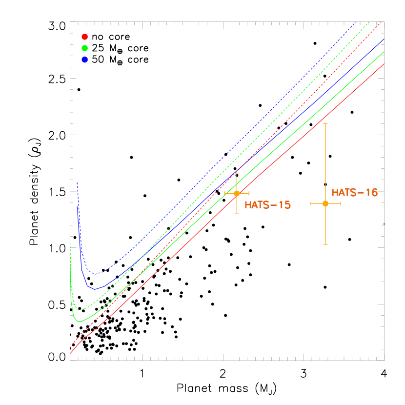
Figure 8.— The HATS-15 and HATS-16 planets (highlighted in orange) are presented in the mass–density diagram of the known transiting planets for which the mass is measured. The superimposed lines represent the expected density of the planet having an inner core of 0, 25 and 50 Earth masses, and calculated for 10 Gyr old planets at 0.02 AU, solid lines, and 0.045 AU, dashed lines (Fortney et al., 2007). To be noticed is that $\sim$2 - 3 $M_{\mathrm{J}}$ transiting planets are much rarer than those in the $\sim$0.1 - 1 $M_{\mathrm{J}}$ mass regime.

The reason of this paucity should be related to different channels that were undertaken by these planets during their formation and migration history. Alternatively, they are simply rarer than the lighter hot Jupiters, as it happens between planets and brown dwarfs. Actually, the existence of the brown-dwarf desert (i.e. companions in the mass range $10-100\,M_{\mathrm{J}}$ are $\sim 1$ order-of-magnitude rarer compared to less massive objects, e.g., Winn & Fabrycky, 2015 and references therein) is by now well ascertained. Finding and characterizing new hot Jupiters is the only key to clarify the causes of the rareness of massive hot Jupiters and the ongoing ground-based surveys, as well as the upcoming (TESS, Ricker et al., 2009) and future (PLATO, Catala & Plato Team, 2006) space missions, are essential for this purpose.

Using the planetary mass–density relations for planets with $M_{\mathrm{p}}\gtrsim 0.4\,M_{\mathrm{J}}$ presented in Bakos et al. (2015), we find that both the planets fall within the predicted range, in particular HATS-15b shows an average density among the planets with the same mass, while HATS-16b lies close to the lower limit of the relation. In addition, comparing the mass and radius of the two planets with the predictions of Fortney et al. (2007), we give some constraints on the presence of an inner heavy core. According to the distance from its parent star, the age of the system and for a fixed planetary mass, the expected radius of the planet is computed in the cases of different internal core masses. We found that HATS-16b is well described by a core-less model, whereas in the case of HATS-15b we expect that it has a very light core. Indeed, we can exclude the case of a massive core as our measurement is only consistent with models predicting a core-mass lower than $50\,M_{\oplus}$ (see Fig. 8).

Comparing HATS-16 b with known planets in the same mass range, we found that the majority of the planets are located far away from their host star having periods greater than 200 days. The eccentricity distribution for those planets seems to be more flat than for the confirmed planets with smaller masses, where there is a slight preference for circular orbits. Howbeit, this can be easily explained taking into account the fact most of those planets have very short periods and therefore are more prone to suffer from circularizations and tidal locking mechanism that result in circular orbits.

In the mass–period parameter space the twin systems to HATS-16 are Kepler-43 (Bonomo et al., 2012) and WASP-10 (Christian et al., 2009). The first system doesn’t show any hint of stellar activity or planet-star interaction, however this might not be surprising given the young age of the system. In the latter case the planet has an eccentric orbit that, assuming a $Q_{*}\sim 10^{5}$ or $\sim 10^{6}$, should have disappeared because of circularizations due to tidal interaction, but still persist indicating some other form of interaction e.g. the presence of an external massive body belonging to the same system.

Although having a mass twice that of Jupiter, HATS-15 b lies in a more populated region of the parameter space than HATS-16 b. There are indeed both long period and short period planets in its mass range that share their average properties with all the other planets. HATS-15 b finds its twin planet in WASP-87A b (Anderson et al., 2014). The main difference between the two planetary systems is that while HATS-15 is a single star, WASP-87 is composed by two stars: the mid-F type host star and a mid-G companion. More over given the different spectral class of the host star HATS-15 b has a less inflated radius than its twin and is therefore denser.

Table 6 Relative radial velocities and bisector spans for HATS-15 and HATS-16.

BJD	RV	$\sigma_{\rm RV}$	BS	$\sigma_{\rm BS}$	Phase	Instrument
(2,456,000$+$)	($\mathrm{m\,s}^{-1}$)	($\mathrm{m\,s}^{-1}$)	($\mathrm{m\,s}^{-1}$)	($\mathrm{m\,s}^{-1}$)
HATS-15
$-188.27661$	$418.77$	$54.00$	$-75.0$	$23.0$	$0.677$	FEROS
$-186.41173$	$418.77$	$32.00$	$16.0$	$15.0$	$0.744$	FEROS
$-185.23774$	$-279.23$	$45.00$	$0.0$	$19.0$	$0.416$	FEROS
$81.70953$	$-270.39$	$131.00$	$-345.0$	$37.0$	$0.176$	Coralie
$82.73890$	$769.61$	$189.00$	$-124.0$	$37.0$	$0.766$	Coralie
$146.71065$	$-344.23$	$75.00$	$-287.0$	$30.0$	$0.373$	FEROS
$162.62586$	$9.77$	$49.00$	$107.0$	$21.0$	$0.481$	FEROS
$167.63696$	$-337.23$	$32.00$	$57.0$	$15.0$	$0.348$	FEROS
$172.74493$	$-468.23$	$34.00$	$27.0$	$15.0$	$0.271$	FEROS
$241.56988$	$212.61$	$126.00$	$-48.0$	$37.0$	$0.657$	Coralie
$400.84394$	$389.77$	$35.00$	$44.0$	$16.0$	$0.801$	FEROS
$404.85903$	$-189.23$	$39.00$	$75.0$	$17.0$	$0.099$	FEROS
$406.82914$	$-261.23$	$43.00$	$71.0$	$19.0$	$0.226$	FEROS
$424.80863$	$48.77$	$41.00$	$10.0$	$18.0$	$0.515$	FEROS
$426.78243$	$138.77$	$85.00$	$10.0$	$34.0$	$0.644$	FEROS
$427.78530$	$-342.23$	$84.00$	$\cdots$	$\cdots$	$0.218$	FEROS
HATS-16
$841.86396$	$-477.43$	$18.00$	$63.0$	$16.0$	$0.355$	FEROS
$844.89323$	$-54.43$	$16.00$	$43.0$	$14.0$	$0.483$	FEROS
$846.85037$	$-465.43$	$14.00$	$44.0$	$13.0$	$0.211$	FEROS
$852.89702$	$-435.43$	$19.0$	$-215$	$16.0$	$0.462$	FEROS
$853.84870$	$439.57$	$23.0$	$-363$	$19.0$	$0.816$	FEROS
$854.90341$	$-482.43$	$19.0$	$-429$	$16.0$	$0.208$	FEROS
$858.68871$	$292.57$	$15.00$	$-36.0$	$14.0$	$0.618$	FEROS
$858.86912$	$500.57$	$16.00$	$23.0$	$14.0$	$0.685$	FEROS
$866.80486$	$342.57$	$17.00$	$69.0$	$15.0$	$0.639$	FEROS
$871.70647$	$-133.43$	$17.00$	$56.0$	$16.0$	$0.464$	FEROS
$908.12221$	$-57.08$	$5.94$	$\cdots$	$\cdots$	$0.019$	HIRES
$909.06821$	$-290.30$	$9.17$	$\cdots$	$\cdots$	$0.371$	HIRES
$910.05021$	$477.26$	$6.37$	$\cdots$	$\cdots$	$0.736$	HIRES
$912.07720$	$-94.72$	$6.24$	$\cdots$	$\cdots$	$0.491$	HIRES
$932.74739$	$-375.43$	$16.00$	$48.0$	$15.0$	$0.185$	FEROS
$942.64274$	$429.57$	$18.00$	$39.0$	$16.0$	$0.868$	FEROS

References

- Anderson et al. (2014) Anderson, D. R., Brown, D. J. A., Collier Cameron, A., et al. 2014, ArXiv e-prints, 1410.3449
- Angus et al. (2015) Angus, R., Aigrain, S., Foreman-Mackey, D., & McQuillan, A. 2015, MNRAS, 450, 1787
- Bakos et al. (2004) Bakos, G., Noyes, R. W., Kovács, G., et al. 2004, PASP, 116, 266
- Bakos et al. (2010) Bakos, G. A., Torres, G., Pál, A., et al. 2010, ApJ, 710, 1724
- Bakos et al. (2013) Bakos, G. A., Csubry, Z., Penev, K., et al. 2013, PASP, 125, 154
- Bakos et al. (2015) Bakos, G. A., Penev, K., Bayliss, D., et al. 2015, ApJ, 813, 111
- Barnes (2007) Barnes, S. A. 2007, ApJ, 669, 1167
- Bayliss et al. (2013) Bayliss, D., Zhou, G., Penev, K., et al. 2013, AJ, 146, 113
- Bayliss et al. (2015) Bayliss, D., Hartman, J. D., Bakos, G. A., et al. 2015, AJ, 150, 49
- Bertelli et al. (2008) Bertelli, G., Girardi, L., Marigo, P., & Nasi, E. 2008, A&A, 484, 815
- Bertin & Arnouts (1996) Bertin, E., & Arnouts, S. 1996, A&AS, 117, 393
- Binney et al. (2000) Binney, J., Dehnen, W., & Bertelli, G. 2000, MNRAS, 318, 658
- Bonfanti et al. (2015) Bonfanti, A., Ortolani, S., & Nascimbeni, V. 2015, ArXiv e-prints, 1511.01744
- Bonomo et al. (2012) Bonomo, A. S., Hébrard, G., Santerne, A., et al. 2012, A&A, 538, A96
- Borucki et al. (2010) Borucki, W. J., Koch, D., Basri, G., et al. 2010, Science, 327, 977
- Brahm et al. (2015) Brahm, R., et al. 2015, in prep.
- Cardelli et al. (1989) Cardelli, J. A., Clayton, G. C., & Mathis, J. S. 1989, ApJ, 345, 245
- Catala & Plato Team (2006) Catala, C., & Plato Team. 2006, in ESA Special Publication, Vol. 1306, ESA Special Publication, ed. M. Fridlund, A. Baglin, J. Lochard, & L. Conroy, 497
- Christian et al. (2009) Christian, D. J., Gibson, N. P., Simpson, E. K., et al. 2009, MNRAS, 392, 1585
- Claret (2004) Claret, A. 2004, A&A, 428, 1001
- Coelho (2014) Coelho, P. R. T. 2014, MNRAS, 440, 1027
- Crane et al. (2010) Crane, J. D., Shectman, S. A., Butler, R. P., et al. 2010, in Society of Photo-Optical Instrumentation Engineers (SPIE) Conference Series, Vol. 7735, Society of Photo-Optical Instrumentation Engineers (SPIE) Conference Series
- Cumming (2004) Cumming, A. 2004, MNRAS, 354, 1165
- Deeg & Doyle (2001) Deeg, H. J., & Doyle, L. R. 2001, in Third Workshop on Photometry, ed. W. J. Borucki & L. E. Lasher, 85
- Dong & Zhu (2013) Dong, S., & Zhu, Z. 2013, ApJ, 778, 53
- Dopita et al. (2007) Dopita, M., Hart, J., McGregor, P., et al. 2007, Ap&SS, 310, 255
- Eastman et al. (2013) Eastman, J., Gaudi, B. S., & Agol, E. 2013, PASP, 125, 83
- Fortney et al. (2007) Fortney, J. J., Marley, M. S., & Barnes, J. W. 2007, ApJ, 659, 1661
- Fressin et al. (2013) Fressin, F., Torres, G., Charbonneau, D., et al. 2013, ApJ, 766, 81
- Fulton et al. (2015) Fulton, B. J., Collins, K. A., Gaudi, B. S., et al. 2015, ApJ, 810, 30
- Greiner et al. (2008) Greiner, J., Bornemann, W., Clemens, C., et al. 2008, PASP, 120, 405
- Hansen & Barman (2007) Hansen, B. M. S., & Barman, T. 2007, ApJ, 671, 861
- Hartman et al. (2012) Hartman, J. D., Bakos, G. A., Béky, B., et al. 2012, AJ, 144, 139
- Howard et al. (2012) Howard, A. W., Marcy, G. W., Bryson, S. T., et al. 2012, ApJS, 201, 15
- Huang et al. (2015) Huang, Y., Liu, X.-W., Yuan, H.-B., et al. 2015, MNRAS, 449, 162
- Husnoo et al. (2012) Husnoo, N., Pont, F., Mazeh, T., et al. 2012, MNRAS, 422, 3151
- Husser et al. (2013) Husser, T.-O., Wende-von Berg, S., Dreizler, S., et al. 2013, A&A, 553, A6
- Jiang et al. (2007) Jiang, I.-G., Yeh, L.-C., Chang, Y.-C., & Hung, W.-L. 2007, AJ, 134, 2061
- Jordán et al. (2014) Jordán, A., Brahm, R., Bakos, G. A., et al. 2014, AJ, 148, 29
- Kaufer & Pasquini (1998) Kaufer, A., & Pasquini, L. 1998, in Society of Photo-Optical Instrumentation Engineers (SPIE) Conference Series, Vol. 3355, Optical Astronomical Instrumentation, ed. S. D’Odorico, 844–854
- Kovács et al. (2005) Kovács, G., Bakos, G., & Noyes, R. W. 2005, MNRAS, 356, 557
- Kovács et al. (2002) Kovács, G., Zucker, S., & Mazeh, T. 2002, A&A, 391, 369
- Mamajek & Hillenbrand (2008) Mamajek, E. E., & Hillenbrand, L. A. 2008, ApJ, 687, 1264
- Mandel & Agol (2002) Mandel, K., & Agol, E. 2002, ApJ, 580, L171
- Marcy & Butler (1992) Marcy, G. W., & Butler, R. P. 1992, PASP, 104, 270
- Marsh (1989) Marsh, T. R. 1989, PASP, 101, 1032
- Maxted et al. (2015) Maxted, P. F. L., Serenelli, A. M., & Southworth, J. 2015, A&A, 577, A90
- Mayor et al. (2011) Mayor, M., Marmier, M., Lovis, C., et al. 2011, ArXiv e-prints, 1109.2497
- Meschiari et al. (2009) Meschiari, S., Wolf, A. S., Rivera, E., et al. 2009, PASP, 121, 1016
- Mohler-Fischer et al. (2013) Mohler-Fischer, M., Mancini, L., Hartman, J. D., et al. 2013, A&A, 558, A55
- Nordström et al. (2004) Nordström, B., Mayor, M., Andersen, J., et al. 2004, A&A, 418, 989
- Pál et al. (2008) Pál, A., Bakos, G. A., Torres, G., et al. 2008, ApJ, 680, 1450
- Penev & Sasselov (2011) Penev, K., & Sasselov, D. 2011, ApJ, 731, 67
- Penev et al. (2013) Penev, K., Bakos, G. A., Bayliss, D., et al. 2013, AJ, 145, 5
- Pollacco et al. (2006) Pollacco, D. L., Skillen, I., Collier Cameron, A., et al. 2006, PASP, 118, 1407
- Pont (2009) Pont, F. 2009, MNRAS, 396, 1789
- Queloz et al. (2001) Queloz, D., Mayor, M., Udry, S., et al. 2001, The Messenger, 105, 1
- Rabus et al. (2015) Rabus, M., et al. 2015, in prep.
- Ricker et al. (2009) Ricker, G. R., Latham, D. W., Vanderspek, R. K., et al. 2009, in , #403.01
- Santos et al. (2013) Santos, N. C., Sousa, S. G., Mortier, A., et al. 2013, A&A, 556, A150
- Schlafly & Finkbeiner (2011) Schlafly, E. F., & Finkbeiner, D. P. 2011, ApJ, 737, 103
- Schlegel et al. (1998) Schlegel, D. J., Finkbeiner, D. P., & Davis, M. 1998, ApJ, 500, 525
- Seager & Mallén-Ornelas (2003) Seager, S., & Mallén-Ornelas, G. 2003, ApJ, 585, 1038
- Soderblom (1983) Soderblom, D. R. 1983, ApJS, 53, 1
- Sozzetti et al. (2007) Sozzetti, A., Torres, G., Charbonneau, D., et al. 2007, ApJ, 664, 1190
- ter Braak (2006) ter Braak, C. J. F. 2006, Statistics and Computing, 16, 239
- Torres et al. (2007) Torres, G., Bakos, G. A., Kovács, G., et al. 2007, ApJ, 666, L121
- Valenti & Fischer (2005) Valenti, J. A., & Fischer, D. A. 2005, ApJS, 159, 141
- Vogt et al. (1994) Vogt, S. S., Allen, S. L., Bigelow, B. C., et al. 1994, in Society of Photo-Optical Instrumentation Engineers (SPIE) Conference Series, Vol. 2198, Instrumentation in Astronomy VIII, ed. D. L. Crawford & E. R. Craine, 362
- Winn & Fabrycky (2015) Winn, J. N., & Fabrycky, D. C. 2015, ARA&A, 53, 409
- Yi et al. (2001) Yi, S., Demarque, P., Kim, Y.-C., et al. 2001, ApJS, 136, 417
- Zacharias et al. (2012) Zacharias, N., Finch, C. T., Girard, T. M., et al. 2012, VizieR Online Data Catalog, 1322, 0
- Zechmeister & Kürster (2009) Zechmeister, M., & Kürster, M. 2009, A&A, 496, 577
- Zhou et al. (2014) Zhou, G., Bayliss, D., Hartman, J. D., et al. 2014, MNRAS, 437, 2831