LAL-15-382

1 Motivation

The first accurate measurement of the $2S_{1/2}^{F=1}-2P_{1/2}^{F=2}$ Lamb shift transition in muonic hydrogen [1] has led, with the help of the currently accepted theoretical formulae (e.g. [2, 3]), to a determination of the proton radius $r_{E}$ with a precision of 0.8 per mil. The proton size puzzle arose from the discrepancy, by five standard deviations, between this result and the CODATA-2010 value [4], which was based on ordinary hydrogen spectroscopy as well as $ep$ scattering. This has stimulated a number of new theoretical and experimental investigations (see e.g. the review [5]). In particular, Antognini at al. [6] have measured both the $\nu_{t}\equiv 2S_{1/2}^{F=1}-2P_{3/2}^{F=2}$ and the $\nu_{s}\equiv 2S_{1/2}^{F=0}-2P_{3/2}^{F=1}$ transitions which has confirmed and refined the previous result on the Lamb shift (increasing the $r_{E}$ discrepancy to $7\sigma$) and further provides an experimental value for the $2S$ hyperfine splitting

$$\Delta E_{HFS}^{exp}=22.8089(51)\ (\hbox{meV})\ .$$ (1)

The hyperfine splitting is interesting as it probes aspects of the proton structure somewhat differently from the Lamb shift. While the influence of the proton radius $r_{E}$ is suppressed, the main structure dependent contribution is proportional to the Zemach radius $r_{Z}$: $\Delta E_{HFS}^{Z}=-0.1621(10)\,r_{Z}$ meV (with $r_{Z}$ in fm), as given in the review [8], and the next main structure dependent contribution is that associated with the forward proton polarizabilities. It has been estimated in ref. [9] as: $\Delta E_{HFS}^{pol}=(8.0\pm 2.6)$ $\mu\hbox{eV}$ (see also  [10]). It is noteworthy that the value of $r_{Z}$ that one determines from the HFS measurement in muonic hydrogen: $r_{Z}=1.082(37)$ fm [6] is in agreement with the value computed in terms of the proton form factors $G_{E}$, $G_{M}$ measured in $ep$ scattering, $r_{Z}=1.086(12)$ fm [11], at the present level of accuracy.

A possible role in muonic hydrogen of light, exotic (universality violating) particles, with vector or axial-vector ($J^{PC}=1^{--},\,=1^{++}$) quantum numbers has been considered [12, 13]. Similarly, the influence of exchanging a light pseudo-scalar particle ($J^{PC}=0^{-+}$) was recently studied in ref. [14]. In that case, the HFS splitting is affected but not the (appropriately defined) Lamb shift.

In this note, we point out that a light pseudo-scalar particle exists within the standard model, the neutral pion, and we perform the exercise to estimate the influence of the one-pion exchange mechanism on $\Delta{E}_{HFS}$. We will show that using chiral symmetry allows one to evaluate the two vertex functions which are needed, represented by blobs in Fig. 1, for small momentum transfer, based on experimental data.

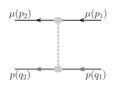
Figure 1: Single pion exchange in the $\mu p\to\mu p$ amplitude

The coupling of the $\pi^{0}$ to a lepton pair proceeds (within the standard model) via two virtual photons. The $\mu p\to\mu p$ one-pion exchange amplitude can also be viewed as a two-photon exchange amplitude. The pion pole in the Compton amplitude $\gamma p\to\gamma p$ contributes to the so-called proton backward spin polarizability $\gamma_{\pi}$ (e.g. [15]). The corresponding contribution in muonic hydrogen is then expected to be suppressed by one power of $\alpha$ as compared to the forward proton polarizability contribution. This explains why the simple mechanism of Fig. 1 does not seem to have been previously considered until very recently [16, 17]. Some enhancement might be expected from the fact that $\gamma_{\pi}$ is numerically large compared to the forward polarizabilities $\alpha_{p}$, $\beta_{p}$ and from the fact that the Yukawa potential has a relatively long range (on the scale of the proton size) which increases the overlap with the atomic wave-functions As a final motivation, let us recall that the $\pi^{0}\mu^{+}\mu^{-}$ coupling plays a significant role among the hadronic contributions to the muon $g-2$ [18] and it is thus of interest to probe the level of sensitivity of muonic hydrogen to this coupling.

2 Pion coupling amplitudes to leptons and to nucleons

2.1 $\pi^{0}$-lepton coupling

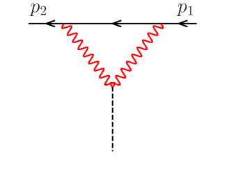
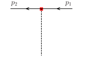
Figure 2: Feynman graphs which generate the $\pi^{0}$-lepton vertex amplitude at leading order in the chiral expansion.

For low momentum transfer, the $P{\ell^{+}}{\ell^{-}}$ vertex amplitude, where $P$ is a light neutral pseudo-scalar meson ($\pi^{0}$ or $\eta$) and $\ell^{\pm}$ is a light lepton ($e^{\pm}$ or $\mu^{\pm}$), can be evaluated in the chiral expansion [19]. At leading order, the amplitude is given from the two diagrams shown on fig. 2. In the one-loop diagram, the $P\gamma\gamma$ vertex is generated by the Wess-Zumino-Witten Lagrangian (see [20], chap. 22)

$${\cal L}_{WZ}=\frac{\alpha}{8\pi F_{\pi}}\epsilon^{\mu\nu\alpha\beta}\big{(}\pi^{0}+{1\over\sqrt{3}}\eta\big{)}\,F_{\mu\nu}F_{\alpha\beta}$$ (2)

with the sign corresponding to the convention $\epsilon^{0123}=1$ (we also use $\gamma^{5}=i\gamma^{0}\gamma^{1}\gamma^{2}\gamma^{3}$). This diagram accounts for the contributions of photons with low energy compared to 1 GeV. The higher energy contributions are parametrized through two chiral coupling constants $\chi_{1}$, $\chi_{2}$ in the Lagrangian [19],

$${\cal L}_{SLW}=\frac{3i{\alpha^{2}}}{32\pi^{2}}\,\bar{\ell}\gamma^{\mu}\gamma^{5}\ell\,\left(\chi_{1}\,{\langle Q^{2}U^{\dagger}D_{\mu}U-Q^{2}UD_{\mu}U^{\dagger}\rangle}+\chi_{2}\,{\langle QU^{\dagger}QD_{\mu}U-QUQD_{\mu}U^{\dagger}\rangle}\right)$$ (3)

where $U$ is the chiral $SU(3)$ matrix,

$$U=\exp\frac{i\Phi}{F_{\pi}},\quad\Phi=\begin{pmatrix}\pi^{0}+\dfrac{\eta}{\sqrt{3}}&\sqrt{2}\,{\pi^{+}}&\sqrt{2}\,{K^{+}}\\ \sqrt{2}\,{\pi^{-}}&-\pi^{0}+\dfrac{\eta}{\sqrt{3}}&\sqrt{2}\,{K^{0}}\\ \sqrt{2}\,{K^{-}}&\sqrt{2}\,{\bar{K}^{0}}&-\dfrac{2\,\eta}{\sqrt{3}}\\ \end{pmatrix}$$ (4)

and

$$D_{\mu}U=\partial_{\mu}U-i(v_{\mu}+a_{\mu})\,U+iU\,(v_{\mu}-a_{\mu})$$ (5)

where $v_{\mu}(\,a_{\mu}$) are external vector (axial-vector) sources (see [21]) and $Q$ is the charge matrix, $Q=diag(2/3,-1/3,-1/3)$. The tree graph shown in fig. 2 is computed from this Lagrangian. The coupling constants $\chi_{1}$, $\chi_{2}$ remove the ultraviolet divergence of the one-loop graph. Assuming the leptons to be on their mass shell, the $P{\ell^{+}}{\ell^{-}}$ vertex amplitude can be expressed in terms of a single Dirac structure,

$$i{\cal T}_{P{\ell^{+}}{\ell^{-}}}=r_{P}\frac{\alpha^{2}m_{\ell}}{2\pi^{2}F_{\pi}}\,{\cal A}_{\ell}((p_{1}-p_{2})^{2})\,\bar{u}_{\ell}(p_{2})\gamma^{5}u_{\ell}(p_{1}),$$ (6)

where $r_{P}=1,\ 1/\sqrt{3}$ if $P=\pi,\,\eta$. In practice, dimensional regularization brings in some scheme dependence because of the presence of the $\gamma^{5}$ matrix. For instance, the amplitudes computed in refs. [19] and [22] differ by a constant. Some discussion of this point can be found in ref. [23]. For definiteness, we will choose the convention of [22], which gives ${\cal A}_{\ell}(s)$ in the form

$${\cal A}_{\ell}(s)=\chi_{P}(\Lambda)+{3\over 2}\log\frac{m_{\ell}^{2}}{\Lambda^{2}}-\frac{5}{2}+C_{\ell}(s),\quad\chi_{P}=-{1\over 4}(\chi_{1}+\chi_{2})\$$ (7)

with

$$C_{\ell}(s)=\frac{1}{\beta_{\ell}(s)}\left[\hbox{Li}_{2}\frac{\beta_{\ell}(s)-1}{\beta_{\ell}(s)+1}+\frac{\pi^{2}}{3}+\frac{1}{4}\log^{2}\frac{\beta_{\ell}(s)+1}{\beta_{\ell}(s)-1}\right],\quad\beta_{\ell}(s)=\sqrt{1-4m_{\ell}^{2}/s}\ .$$ (8)

Using $\overline{MS}$ renormalization, the coupling constant combination $\chi_{P}$ becomes scale dependent with $d/d\Lambda\chi_{P}(\Lambda)=3/\Lambda$, which ensures that ${\cal A}_{\ell}$ is scale independent.

The value of $\chi_{P}(\Lambda)$ must be determined from experiment. For this purpose, we can use either $\pi^{0}\to e^{+}e^{-}$ which was measured recently by the KTeV collaboration [24] or $\eta\to\mu^{+}\mu^{-}$ (see [25]). It is convenient to consider the ratio $R_{P}=\Gamma(P\to{\ell^{+}}{\ell^{-}})/\Gamma(P\to\gamma\gamma)$ which should be less sensitive to higher order chiral corrections than the individual modes. It is expressed as follows, in terms of the amplitude ${\cal A}_{\ell}$,

$$R_{P}=\frac{2\,\alpha^{2}m_{\ell}^{2}}{\pi^{2}m_{P}^{2}}\,\beta_{\ell}(m^{2}_{P})\,\left|{\cal A}_{\ell}(m^{2}_{P})\right|^{2}\ \ .$$ (9)

In the case of the $\pi^{0}$, the quantity measured experimentally is the branching ratio for the decay mode $\pi^{0}\to e^{+}e^{-}(\gamma)$, including photons in the final state such that $s_{e^{+}e^{-}}\geq 0.95m^{2}_{\pi^{0}}$. The ratio which interest us, $R_{\pi^{0}}$, can be deduced from this result by removing the bremsstrahlung and the associated radiative corrections. These have been revised recently in ref. [26]. Using the results of that work, one deduces

$$R_{\pi^{0}}^{exp}=(6.96\pm 0.36)\cdot 10^{-8}\ .$$ (10)

There are two solutions for $\chi_{P}$ which correspond to this experimental result

$$\begin{array}[]{l}a)\,\chi_{P}(m_{\rho})=4.51\pm 0.97\\[2.0pt] b)\,\chi_{P}(m_{\rho})=-19.41\pm 0.97\\ \end{array}$$ (11)

(in which the scale was set to $\Lambda=m_{\rho}=0.774$ GeV). In order to decide on which solution to choose, we can compare with the model proposed in ref. [22]. It is based on a rigorous sum rule which holds in the large $N_{c}$ limit of QCD and the approximation of retaining only the lightest resonance in the sum. This model gives,

$$\chi_{P}^{LMD}(\Lambda)=\frac{11}{4}-\frac{3}{2}\log{m_{\rho}^{2}\over\Lambda^{2}}-\frac{4\pi^{2}F_{\pi}^{2}}{m_{\rho}^{2}}$$ (12)

and the uncertainty was estimated in ref. [22] to be of the order of 40%. Thus, one has

$$\chi_{P}^{LMD}(m_{\rho})\simeq 2.2\pm 0.8\ .$$ (13)

This result lies within one sigma of solution $a)$ and is not compatible with solution $b)$. This argument suggests that solution $a)$ is more likely to be the physically correct one.

Alternatively, we can determine the coupling constant $\chi_{P}$ from the decay mode of the $\eta$ meson, $\eta\to\mu^{+}\mu^{-}$ for which the experimental branching fraction is (see [25]): $BF(\eta\to\mu^{+}\mu^{-})=(5.8\pm 0.8)\cdot 10^{-6}$ leading to

$$R_{\eta}^{exp}=(1.47\pm 0.20)\cdot 10^{-5}$$ (14)

There are again two solutions for $\chi_{P}$ corresponding to this experimental result,

$$\begin{array}[]{l}a^{\prime})\,\chi_{P}(m_{\rho})=1.69\pm 0.87\\[2.0pt] b^{\prime})\,\chi_{P}(m_{\rho})=7.96\pm 0.87\ .\end{array}$$ (15)

None of these solutions is compatible with $b)$ of eq. (11): one can therefore safely conclude that solution $b)$ must be eliminated. We can also eliminate $b^{\prime})$ which is not compatible with the model estimate (12) while $a^{\prime})$ is. It seems reasonable, for our purposes, to perform an average of the $a)$ and $a^{\prime})$ values and thus use

$$\chi_{P}(m_{\rho})=3.10\pm 1.50\ ,$$ (16)

where we have slightly rescaled the error such that the two central values of $a)$ and $a^{\prime})$ lie within the error.

2.2 $\pi^{0}$-proton coupling

At leading order in the chiral expansion, the pion-nucleon coupling is given, at tree level, from the chiral Lagrangian [27]

$${\cal L}_{\pi NN}=\bar{\psi}\left(i\gamma^{\mu}\Delta_{\mu}-m_{N}+i{g_{A}\over 2}\gamma^{\mu}\gamma^{5}u^{\dagger}D_{\mu}Uu^{\dagger}\right)\psi,\quad$$ (17)

where $U$ is the $SU(2)$ chiral matrix here, $u=\sqrt{U}$, and

$$\Delta_{\mu}=\partial_{\mu}+\Gamma_{\mu},\quad\Gamma_{\mu}=\frac{1}{2}[u^{\dagger},\partial_{\mu}u]-\frac{1}{2}iu^{\dagger}(v_{\mu}+a_{\mu})u-\frac{1}{2}iu(v_{\mu}-a_{\mu})u^{\dagger}\$$ (18)

$v_{\mu}$ ($a_{\mu}$) being external vector (axial-vector) sources and $\psi$ is an isospin spinor containing the proton and the neutron,

$$\psi=\begin{pmatrix}\psi_{p}\\ \psi_{n}\\ \end{pmatrix}\ .$$ (19)

The coupling constant $g_{A}$ in the Lagrangian. (17) is easily identified as the axial charge of the proton and also controls the neutron-proton matrix element of the charged axial current,

$$\lim_{q^{\prime}=q}{\langle p(q^{\prime})|\bar{u}\gamma^{\mu}\gamma^{5}d|n(q)\rangle}=g_{A}\,\bar{u}_{p}(q)\gamma^{\mu}\gamma^{5}u_{n}(q)\ .$$ (20)

It is determined from neutron beta decay experiments to have the following positive value [25]

$$g_{A}=1.2723\pm 0.0023$$ (21)

The pion-proton vertex amplitude is then deduced from the Lagrangian (17) to be

$$i{\cal T}_{\pi pp}=-g_{\pi pp}\,\bar{u}_{p}(q_{2})\gamma^{5}u_{p}(q_{1}),\qquad g_{\pi pp}=\frac{g_{A}m_{p}}{F_{\pi}}$$ (22)

The expression of the coupling constant $g_{\pi pp}$ at leading chiral order, in terms of $g_{A}$, $m_{p}$ and $F_{\pi}$, as it appears in the above expression is, of course, the content of the Nambu-Goldberger-Treiman relation (e.g. [20] chap. 19). It is known that the higher order chiral corrections to this relation do not exceed a few percent.

3 Energy shifts in muonic hydrogen

3.1 $q^{2}=0$ approximation

Having determined the $\pi^{0}\mu\mu$ vertex (eq. (6)) and the $\pi^{0}pp$ vertex (eq. (22)) it is straightforward to derive the muon-proton scattering amplitude, $\mu(p_{1})p(q_{1})\to\mu(p_{2})p(q_{2})$ associated with one-pion exchange (Fig. 1)

$${\cal T}_{\mu p}=-{4m_{\mu}m_{p}\,\alpha^{2}g_{A}{\cal A}_{\mu}((p_{1}-p_{2})^{2})\over 8\pi^{2}F_{\pi}^{2}}{\bar{u}_{\mu}(p_{2})\gamma^{5}u_{\mu}(p_{1})\,\bar{u}_{p}(q_{2})\gamma^{5}u_{p}(q_{1})\over(p_{1}-p_{2})^{2}-m_{\pi}^{2}}$$ (23)

For our purposes, we can consider that both the muon and the proton are non-relativistic, therefore

$$(p_{1}-p_{2})^{2}=(q_{1}-q_{2})^{2}\simeq-(\vec{p}_{1}-\vec{p}_{2})^{2}\equiv-q^{2}\ .$$ (24)

At first, let us make the approximation to set $q^{2}=0$ in the vertex function ${\cal A}_{\mu}$. We then obtain the non-relativistic Yukawa potential in momentum space,

$$V_{\mu p}(\vec{q})=-\frac{{\cal T}_{\mu p}}{4m_{\mu}m_{p}}=\lambda\,{\cal A}_{\mu}(0)\,\frac{\vec{\sigma}_{\mu}\cdot\vec{q}\,\,\vec{\sigma}_{p}\cdot\vec{q}}{q^{2}+m_{\pi}^{2}},\quad\lambda={\alpha^{2}g_{A}\over 8\pi^{2}F_{\pi}^{2}}$$ (25)

The contributions to the atomic energy shifts are most easily performed by Fourier transforming to configuration space,

$$V_{\mu p}(\vec{r})=\tilde{\lambda}\,\left[\vec{\sigma}_{\mu}\cdot\vec{\sigma}_{p}\,V_{SS}(\vec{r})+S_{12}\,V_{T}(r)\right],\quad\tilde{\lambda}=-\lambda\,{\cal A}_{\mu}(0)\,\frac{m_{\pi}^{2}}{12\pi}$$ (26)

where $S_{12}=3\,\vec{\sigma}_{\mu}\cdot\hat{r}\,\vec{\sigma}_{p}\cdot\hat{r}-\vec{\sigma}_{\mu}\cdot\vec{\sigma}_{p}$ is the so-called tensor operator, and

$$V_{SS}(\vec{r})=\frac{\exp(-m_{\pi}r)}{r}-\frac{4\pi}{m_{\pi}^{2}}\delta^{3}(\vec{r}),\quad$$

$$V_{T}(r)=\left(1+\frac{3}{m_{\pi}r}+\frac{3}{m_{\pi}^{2}r^{2}}\right)\,\frac{\exp(-m_{\pi}r)}{r}\ .$$ (27)

Making use of the average result (16) for $\chi_{P}$, one obtains the following values for ${\cal A}_{\mu}(0)$ and for the overall coupling $\tilde{\lambda}$ in muonic hydrogen

$${\cal A}_{\mu}(0)=-5.37\pm 1.5\ ,\quad\tilde{\lambda}=(2.61\pm 0.49)\cdot 10^{-7}\ .$$ (28)

We can now compute the energy shifts of muonic hydrogen caused by the one-pion exchange amplitude. We will consider both the 2S and 2P energy shifts for completeness, the relevant radial Coulomb wave-functions are,

$$\psi_{2S}(r)={1\over\sqrt{2}}\exp\left(-{\mu\alpha r\over 2}\right)(1-{\mu\alpha r\over 2}),\ \psi_{2P}(r)={1\over 2\sqrt{6}}\exp\left(-{\mu\alpha r\over 2}\right)\mu\alpha r$$ (29)

where $\mu$ is the muon-proton reduced mass $1/\mu=1/m_{\mu}+1/m_{p}$. From these, one computes the expectation values of the components $V_{SS}$ and $V_{T}$ of the Yukawa potential. For the $S$-wave, firstly, one has

$${\langle 2S|V_{SS}|2S\rangle}\equiv Y_{S}(m_{\pi})=-\frac{(\mu\alpha)^{4}}{m_{\pi}^{3}}\,\frac{8+11\tilde{\alpha}+8\tilde{\alpha}^{2}+2\tilde{\alpha}^{3}}{4(1+\tilde{\alpha})^{4}},\quad\tilde{\alpha}=\frac{\mu\alpha}{m_{\pi}}\,\ .$$ (30)

When computing the expectation value in the $2S$ state, the contribution from the delta function in the potential $V_{SS}$ cancels the leading term in $\alpha$ from the contribution of the first piece. As a result of this cancellation, $Y_{S}$ scales as $\alpha^{4}$ and has a negative sign. For the 2P states, one has

$${\langle 2P|V_{SS}|2P\rangle}\equiv Y_{P}=m_{\pi}\tilde{\alpha}^{5}\,\frac{1}{4(1+\tilde{\alpha})^{4}}$$

$${\langle 2P|V_{T}|2P\rangle}\equiv T_{P}=m_{\pi}\tilde{\alpha}^{5}\,\frac{5+4\tilde{\alpha}+\tilde{\alpha}^{2}}{8(1+\tilde{\alpha})^{4}}$$ (31)

Table 1 lists the expressions for the shifts in the 2P and the 2S states of muonic hydrogen in terms of the integrals $Y_{S}$, $Y_{P}$, $T_{P}$ and the overall coupling $\tilde{\lambda}$ (given in eqs. (26) and  (28)) as well as the central numerical values. The contributions to the $2P_{3/2}$ states is particularly suppressed because the leading terms in $\alpha$ cancel in the combination $Y_{P}-{2\over 5}T_{P}$. Finally, in the $q^{2}=0$ approximation, the contribution from single pion exchange to the $2S$ hyperfine splitting in muonic hydrogen is

$$\Delta E_{HFS}^{\pi}=-(0.19\pm 0.05)\ \mu\hbox{eV}\ ,$$ (32)

which is small but not irrelevant. In contrast, the contributions to the HFS in the 2P states, as can be deduced from table 1 are too small to be of physical relevance. Our result  (32) disagrees with the one quoted in ref. [16] which uses the same approximation. We could trace the origin of the discrepancy, essentially, to an incorrect coefficient for the delta function in the Yukawa potential.

State	Expression	Value ($\mu$eV)
$2P^{F=2}_{3/2}$	$\tilde{\lambda}\,\left(Y_{P}-{2\over 5}T_{P}\right)$	$-1.3\,10^{-7}$
$2P^{F=1}_{3/2}$	$-{5\over 3}\tilde{\lambda}\,\left(Y_{P}-{2\over 5}T_{P}\right)$	$2.1\,10^{-7}$
$2P^{F=1}_{1/2}$	$-{1\over 3}\tilde{\lambda}\,\left(Y_{P}-4\,T_{P}\right)$	$0.9\,10^{-4}$
$2P^{F=0}_{1/2}$	$\tilde{\lambda}\,\left(Y_{P}-4\,T_{P}\right)$	$-2.8\,10^{-4}$
$2S^{F=1}_{1/2}$	$\tilde{\lambda}\,Y_{S}$	-0.049
$2S^{F=0}_{1/2}$	$-3\,\tilde{\lambda}\,Y_{S}$	0.146

Table 1: Contributions from the single pion exchange amplitude to the $2S$ and the $2P$ energy levels in muonic hydrogen

3.2 Influence of the vertex functions momentum dependence

The results quoted above were obtained setting $q^{2}=0$ in the vertex function ${\cal A}_{\mu}$. It was pointed out in ref. [17] that this is not a good approximation. Plotting ${\cal A}_{\mu}(-q^{2})$ (see fig. 3) shows indeed that the vertex function has a strong cusp at $q^{2}=0$ which induces a rapid variation. In the following we evaluate the corrections induced by the $q^{2}$ variation of ${\cal A}_{\mu}$. This is easily done by using the dispersion relation representation of the function ${\cal A}_{\mu}(-q^{2})$,

$${\cal A}_{\mu}(-q^{2})={\cal A}_{\mu}(0)-\frac{q^{2}}{\pi}\int_{0}^{\infty}ds^{\prime}\,\frac{{\rm Im\,}{\cal A}_{\mu}(s^{\prime})}{s^{\prime}(s^{\prime}+q^{2})}\ .$$ (33)

For small values of $q^{2}$ (compared to 1 $\rm{GeV}^{2}$) we can use the leading order chiral approximation which gives, for the imaginary part [19],

$$\begin{array}[]{lll}{\rm Im\,}{\cal A}_{l}(s^{\prime})=&-\pi\,\dfrac{\arctan{\sqrt{4m_{l}^{2}/s^{\prime}-1}}}{\sqrt{4m_{l}^{2}/s^{\prime}-1}}&\quad(s^{\prime}\leq 4m_{l}^{2})\\[14.22636pt] {\rm Im\,}{\cal A}_{l}(s^{\prime})=&-\pi\,\dfrac{\hbox{arctanh}\sqrt{1-4m_{l}^{2}/s^{\prime}}}{\sqrt{1-4m_{l}^{2}/s^{\prime}}}&\quad(s^{\prime}\geq 4m_{l}^{2})\\ \end{array}$$ (34)

(which is easily verified to be reproduced by the explicit expression (7) (8) of ${\cal A}_{l}$). Beyond the low $q^{2}$ region, estimates of the behaviour of ${\cal A}_{\mu}$ may be obtained based on modellings of the $\pi^{0}\gamma^{*}\gamma^{*}$ form factor (e.g. [28, 29] for recent work, see also [30] were a list of references to earlier work can be found). We will not consider these in detail here and content ourselves with a simple estimate of the role of the $q^{2}\mathrel{\raise 0.99025pt\hbox{$>$}\kern-7.7778pt\lower 2.58334pt\hbox{$\sim$}}1$ $\rm{GeV}^{2}$ region, taking into account the $q^{2}$ dependence attached to the $\pi pp$ vertex. In this case, a weak cusp is expected from the three pions threshold at $q^{2}=-9m_{\pi}^{2}$ and the $q^{2}$ dependence is expected to be smooth in the $q^{2}>0$ region. Models of the nucleon-nucleon interaction suggest a simple approximation for the behaviour in this region [31],

$$g_{\pi pp}(-q^{2})\simeq\frac{\Lambda_{\pi}^{2}}{\Lambda_{\pi}^{2}+q^{2}}\,g_{\pi pp}(0)$$ (35)

with $\Lambda_{\pi}\simeq 1.3$ GeV.

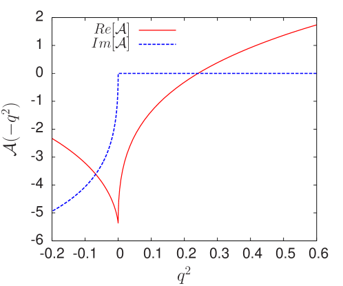
Figure 3: Vertex function ${\cal A}_{\mu}$ as a function of $q^{2}$.

We can now write the $\mu p$ potential, taking into account a more complete picture of the momentum dependence, as

$$V_{\mu p}(q^{2})=\lambda\,\frac{\Lambda_{\pi}^{2}}{\Lambda_{\pi}^{2}+q^{2}}\,\frac{{\cal A}_{\mu}(-q^{2})\,\vec{\sigma}_{\mu}\cdot\vec{q}\,\vec{\sigma}_{p}\cdot\vec{q}}{q^{2}+m_{\pi}^{2}}$$ (36)

(where $\lambda$ is given in eq. (25).) From this, it is not difficult to compute the Fourier transform, using the representation (33) for ${\cal A}_{\mu}(-q^{2})$, and then the expectation values using the formulae of the preceding section. The result for the $2S$ states can be written in the form,

$${\langle 2S|V_{\mu p}|2S\rangle}={\langle\sigma_{\mu}\cdot\sigma_{p}\rangle}\,\left(-{\cal A}_{\mu}(0)+\delta{\cal A}_{1}+\delta{\cal A}_{2}\right)\lambda\,\frac{m_{\pi}^{2}}{12\pi}Y_{S}(m_{\pi})$$ (37)

where the two corrective terms $\delta{\cal A}_{1}$, $\delta{\cal A}_{2}$ have the following expressions

$$\delta{\cal A}_{1}={\cal A}_{\mu}(0)\,\frac{m_{\pi}}{\Lambda_{\pi}+m_{\pi}}$$ (38)

and

$$\delta{\cal A}_{2}=\frac{2}{\pi}\int_{0}^{\infty}dx\, \frac{{\rm Im\,}{\cal A}_{\mu}(m_{\pi}^{2}x^{2})}{x(x^{2}-1)}\bigg{[}\frac{x^{4}}{1-R_{\pi}\,x^{2}}\frac{Y_{S}(m_{\pi}x)}{Y_{S}(m_{\pi})}$$

$$-\frac{1}{1-R_{\pi}}\left(\frac{x^{2}-1}{(1-R_{\pi}\,x^{2})R_{\pi}}\frac{Y_{S}(\Lambda_{\pi})}{Y_{S}(m_{\pi})}+1\right)\bigg{]}$$ (39)

with $R_{\pi}=m_{\pi}^{2}/\Lambda_{\pi}^{2}$. This expression agrees with the result of ref. [17] in the limit $\Lambda_{\pi}\to\infty$ and using the leading order approximation in $\alpha$ of the function $Y_{S}$ (which is valid except when $x$ is very close to zero). Fig. 4 shows that the integrand in eq. (3.2) is peaked at $x=0$. The effect of $\Lambda_{\pi}$ is essentially to cutoff the integration region $x>\Lambda_{\pi}/m_{\pi}$ which reduces the size of $\delta{\cal A}_{2}$ by 30% approximately. Using the numerical result (28) for ${\cal A}_{\mu}(0)$ we find, for the two corrective terms induced by the $q^{2}$ dependence of the vertices,

$$\delta{\cal A}_{1}\simeq-0.52,\quad\delta{\cal A}_{2}\simeq-2.30$$ (40)

which reduce the result based on ${\cal A}_{\mu}(0)$ by roughly 50%. It seems reasonable to affect an uncertainty of $\simeq 30\%$ to these corrective terms. We thus arrive at the following final estimate for the $2S$ hyperfine splitting induced by the exchange of one pion in muonic hydrogen,

$$\Delta{E}^{\pi}_{HFS}=-(0.09\pm 0.06)\ \mu\rm{eV}\ .$$ (41)

The magnitude of this result is compatible with that obtained in ref. [17] within the errors.

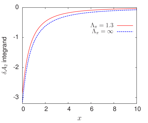
Figure 4: Integrand of the corrective term $\delta{\cal A}_{2}$ given in eq. (3.2).

4 Conclusions

The recent measurement of the 2S HFS in muonic hydrogen [6] incites one to try to improve the theoretical evaluations of the strong interaction effects, in order to reduce the error in the determination of the Zemach radius $r_{Z}$. In this context, we have considered here the “simple” one-pion exchange (Yukawa) contribution. We have indicated how to compute this contribution based on experimental results on $\pi^{0}\to e^{+}e^{-}$, $\eta\to\mu^{+}\mu^{-}$ and the associated low energy chiral expansion as developed, in this sector, in ref. [19]. The use of chiral symmetry is important in order to properly fix the signs of the relevant $\pi\ell\ell$ and $\pi NN$ coupling constants and is also necessary in order to perform low-momentum expansions at the vertices. The final result for the contribution of one-pion exchange to the HFS is given in eq. (41). It has a magnitude comparable to the smallest contributions which are already taken into account in the theoretical evaluation of the HFS (see the list of 28 contributions collected in table 3 of ref. [8]). At present, however, the main source of uncertainty affecting the strong interaction effects in the 2S HFS is that attached to the proton forward polarizabilities.

References

- [1] R. Pohl et al., Nature 466, 213 (2010)
- [2] K. Pachucki, Phys. Rev. A53, 2092 (1996)
- [3] E. Borie, Phys. Rev. A71, 032508 (2005), physics/0410051
- [4] P.J. Mohr, B.N. Taylor, D.B. Newell, Rev. Mod. Phys. 84, 1527 (2012), 1203.5425
- [5] C.E. Carlson, Prog. Part. Nucl. Phys. 82, 59 (2015), 1502.05314
- [6] A. Antognini, F. Nez, K. Schuhmann, F.D. Amaro, F. Biraben et al., Science 339, 417 (2013)
- [7] A.P. Martynenko, Phys. Atom. Nucl. 71, 125 (2008), hep-ph/0610226
- [8] A. Antognini, F. Kottmann, F. Biraben, P. Indelicato, F. Nez, R. Pohl, Annals Phys. 331, 127 (2013), 1208.2637
- [9] C.E. Carlson, V. Nazaryan, K. Griffioen, Phys. Rev. A78, 022517 (2008), 0805.2603
- [10] R.N. Faustov, A.P. Martynenko, Eur. Phys. J. C24, 281 (2002)
- [11] V. Nazaryan, C.E. Carlson, K.A. Griffioen, Phys. Rev. Lett. 96, 163001 (2006), hep-ph/0512108
- [12] V. Barger, C.W. Chiang, W.Y. Keung, D. Marfatia, Phys. Rev. Lett. 106, 153001 (2011), 1011.3519
- [13] S.G. Karshenboim, D. McKeen, M. Pospelov, Phys. Rev. D90(7), 073004 (2014), [Addendum: Phys. Rev.D90,no.7,079905(2014)], 1401.6154
- [14] W.Y. Keung, D. Marfatia, Phys. Lett. B746, 315 (2015), 1501.00455
- [15] D. Drechsel, T. Walcher, Rev. Mod. Phys. 80, 731 (2008), 0711.3396
- [16] H.Q. Zhou, H.R. Pang, Phys. Rev. A92(3), 032512 (2015)
- [17] F. Hagelstein, V. Pascalutsa (2015), 1511.04301
- [18] M. Knecht, A. Nyffeler, Phys. Rev. D65, 073034 (2002), hep-ph/0111058
- [19] M.J. Savage, M.E. Luke, M.B. Wise, Phys. Lett. B291, 481 (1992), hep-ph/9207233
- [20] S. Weinberg, The quantum theory of fields. Vol. 2: Modern applications (Cambridge University Press, 2013), ISBN 9781139632478, 9780521670548, 9780521550024
- [21] J. Gasser, H. Leutwyler, Nucl.Phys. B250, 465 (1985)
- [22] M. Knecht, S. Peris, M. Perrottet, E. de Rafael, Phys. Rev. Lett. 83, 5230 (1999), hep-ph/9908283
- [23] M.J. Ramsey-Musolf, M.B. Wise, Phys. Rev. Lett. 89, 041601 (2002), hep-ph/0201297
- [24] E. Abouzaid et al. (KTeV), Phys. Rev. D75, 012004 (2007), hep-ex/0610072
- [25] K.A. Olive et al. (Particle Data Group), Chin. Phys. C38, 090001 (2014)
- [26] P. Vasko, J. Novotny, JHEP 10, 122 (2011), 1106.5956
- [27] J. Gasser, M.E. Sainio, A. Svarc, Nucl. Phys. B307, 779 (1988)
- [28] A.E. Dorokhov, M.A. Ivanov, S.G. Kovalenko, Phys. Lett. B677, 145 (2009), 0903.4249
- [29] P. Masjuan, P. Sanchez-Puertas (2015), 1504.07001
- [30] L. Ametller, A. Bramon, E. Masso, Phys. Rev. D48, 3388 (1993), hep-ph/9302304
- [31] R. Machleidt, K. Holinde, C. Elster, Phys. Rept. 149, 1 (1987)