Phase-field study of electrochemical reactions at exterior and interior interfaces in Li-Ion battery electrode particles

Abstract

To study the electrochemical reaction on surfaces, phase interfaces, and crack surfaces in the lithium ion battery electrode particles, a phase-field model is developed, which describes fracture in large strains and anisotropic Cahn-Hilliard-Reaction. Thereby the concentration-dependency of the elastic properties and the anisotropy of diffusivity are also considered. The implementation in 3D is carried out by isogeometric finite element methods in order to treat the high order terms in a straightforward sense. The electrochemical reaction is modeled through a modified Butler-Volmer equation to account for the influence of the phase change on the reaction on exterior surfaces. The reaction on the crack surfaces is considered through a volume source term weighted by a term related to the fracture order parameter. Based on the model, three characteristic examples are considered to reveal the electrochemical reactions on particle surfaces, phase interfaces, and crack surfaces, as well as their influence on the particle material behavior. Results show that the ratio between the timescale of reaction and the diffusion can have a significant influence on phase segregation behavior, as well as the anisotropy of diffusivity. In turn, the distribution of the lithium concentration greatly influences the reaction on the surface, especially when the phase interfaces appear on exterior surfaces or crack surfaces. The reaction rate increases considerably at phase interfaces, due to the large lithium concentration gradient. Moreover, simulations demonstrate that the segregation of a Li-rich and a Li-poor phase during delithiation can drive the cracks to propagate. Results indicate that the model can capture the electrochemical reaction on the freshly cracked surfaces.

capbtabboxtable[][]

1 Introduction

Lithium ion batteries, with their high energy densities and light-weight designs, have found wide applications in portable electronics and electric vehicles. A typical lithium ion battery cell is illustrated in Figure 1. The current collectors and the binders between the electrodes (not depicted here) conduct the electrons, while the separator only permits the diffusion of lithium ions. The anode and cathode particles are surrounded by the electrolyte. Lithium ions intercalate into the electrodes through electrochemical reactions on the surface of the particles.

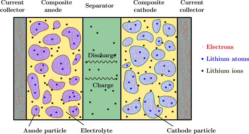
Figure 1: Schematic of a lithium-ion battery cell.

In the electrochemical system of a battery, the reaction rate is a key point since it is directly related to the charging/discharging performance of a battery. The phenomenological Butler-Volmer (BV) equation, which is based on a dilute solution model, may not be able to account for a separation of phases with different Li concentrations in materials, such as silicon and LiFePO₄. In the work of Singh et al. [1], a generalized BV kinetics model was proposed, which includes the influence of the phase transition on the surface reaction in a 1D case. Based on this model, Bai et al. [2] discussed the suppression of the phase segregation under large reaction rate. The two dimensional case, which also coupled the Cahn-Hilliard bulk diffusion was studied by Dargaville and Farrell [3]. Using different limits of the 1D case, they discussed when the orthotropic diffusivity becomes more isotropic. In the mechanically coupled modeling, there has also been a tendency recently to treat the electrochemical reaction on the surface directly through the BV equation rather than simply to replace the reaction by a source of constant or time dependent flux [4, 5].

The mechanical degradation of the electrode particle is widely believed to be closely related to the failure of the batteries and has been intensively studied in various chemo-mechanical coupled models [6, 7, 8, 9]. However, those models mainly treat the diffusion process as in a dilute solution, where the concentration smoothly changes with the incoming/outgoing flux, accompanied by a homogeneous “breathing-like” expansion and shrinkage of the particle, which will hardly lead to the failure of the electrode particles. In the work of Huttin et al. [10] and Walk et al. [11], Cahn-Hilliard equation was employed to investigate the stress state and compared it with the case of a dilute solution. The diffusion process was treated as isotropic in both works. However, as Rohrer et al. [12, 13] have pointed out from first principle calculations, the anisotropic volumetric expansion in Silicon will indeed initiate cracking, especially in large particles, where the segregation between amorphous and crystalline silicon phases can not be suppressed. Moreover, in positive electrode materials such as LiFePO₄, striped phase boundaries have observed by Chen et al. [14, 15] because of strong anisotropy and phase segregation. It demonstrates the necessity to employ a Cahn-Hilliard model and to consider the anisotropic diffusion property coupled with large deformations in describing the bulk behavior of the particle.

The dynamics of crack propagation in lithium ion battery electrode particles has long been a challenge. Recently, as the concept of phase-field modeling finds more applications in different disciplines, phase-field methods are also introduced to predict the crack propagation coupled with diffusion. In the phase-field fracture models, the damaged and undamaged materials are considered as two different phases, indicated by the distinct values of the order parameter. Schneider et al. [16] proposed a model coupling the mechanics with a general multiphase and multicomponent phase-field approach to describe the diffusion and crack propagation in brittle materials. Liang et al. [17] developed a phase-field model to predict the crack evolution in LiFePO₄ cathode nanoparticles in of Li-ion batteries. Concurrently, the phase-field fracture simulation in silicon anodes is also carried out by Zuo et al. [18]. Recently, Miehe et al. [19] conducted a comprehensive study on chemical reaction on fracture surfaces in the framework of phase-field fracture modeling, in addition to the reactions on exterior surfaces.

In this paper, the authors propose a phase-field model which accounts for electrochemical reactions on different interior and exterior of phases and crack surfaces based on the fully coupled Cahn-Hilliard-Reaction (CHR) model proposed in the work of Bazant [20]. To meet the demand of higher-order continuity arising from the Cahn-Hilliard equation, isogeometric analysis is employed.

The paper is organized as follows. In section 2, the phase-field fracture model coupled with anisotropic Cahn-Hilliard-Reaction problem in large strain model is formulated. The modeling of electrochemical reactions on the surface, phase interface, and on the crack surface is shown in section 3. Numerical details are given in section 4. Finally, three examples are given in section 5 to discuss the reaction rate, anisotropic diffusion, and the reaction on the crack surface.

2 Phase-field model of fracture and phase separation

2.1 Kinematics

According to continuum theory, the material coordinates $\displaystyle\mathbf{X}$ label each material point, while the spatial coordinates $\displaystyle\mathbf{x}$ denote points in the space. The motion of the body can be described by tracking the spatial coordinates of the material points at time $\displaystyle t$, i.e. $\displaystyle\mathbf{x}=\bm{\phi}(\mathbf{X},t)$. The deformation gradient at a given time is then defined as

$$\mathbf{F}=\bm{\nabla}_{\!\mathrm{R}}\,\bm{\phi}$$ (1)

in which $\displaystyle\bm{\nabla}_{\!\mathrm{R}}$ denotes the gradient with respect to the material point $\displaystyle\mathbf{X}$ in the reference (material) configuration. The deformation gradient is multiplicatively decomposed into two parts:

$$\mathbf{F}=\mathbf{F}^{e}\mathbf{F}^{c},$$ (2)

where $\displaystyle\mathbf{F}^{e}$ denotes the elastic distortion, and $\displaystyle\mathbf{F}^{c}$ the (de-)intercalation-induced deformation. The (de-)intercalation-induced deformation is usually assumed to be volumetric, and it can be further defined as

$$\mathbf{F}^{c}=\left(J^{c}\right)^{\frac{1}{3}}\mathbf{1},\quad\mathrm{with}\;\;J^{c}=1+\Omega c_{\mathrm{R}}$$ (3)

in which $\displaystyle c_{\mathrm{R}}(\mathbf{X},t)$ is the molar concentration per unit volume in the reference configuration, and $\displaystyle\Omega$ is the constant partial molar volume. Applying the normalization with respect to the maximum concentration $\displaystyle\mathrm{c}_{\mathrm{max}}$,

$$c={c_{\mathrm{R}}}/{\mathrm{c}_{\mathrm{max}}},\quad\,\Omega^{\ast}={\Omega}{\mathrm{c}_{\mathrm{max}}}.$$ (4)

one has

$$J^{c}=1+\Omega^{\ast}c.$$ (5)

On the other hand, one can also define the volumetric part of the elastic contribution $\displaystyle\mathbf{F}^{e}$,

$$J^{e}=\mathrm{det}\,\mathbf{F}^{e}=J/J^{c},\quad\mathrm{with}\;\;J=\mathrm{det}\,\mathbf{F}.$$ (6)

The right Cauchy-Green deformation tensors are

$$\mathbf{C}=\mathbf{F}^{\mathrm{T}}\mathbf{F},\quad\mathbf{C}^{e}=(\mathbf{F}^{e})^{\mathrm{T}}\mathbf{F}^{e}=\left(J^{c}\right)^{-\frac{2}{3}}\mathbf{C}.$$ (7)

Due to volumetric feature of $\displaystyle\mathbf{F}^{c}$, the deviatoric part of the total deformation equals that of the elastic deformation, i.e.,

$$\bar{\mathbf{C}}=\bar{\mathbf{C}}^{e},\quad\mathrm{with}\,\,\,\bar{\mathbf{C}}=J^{-\frac{2}{3}}\mathbf{C},\quad\bar{\mathbf{C}}^{e}=(J^{e})^{-\frac{2}{3}}\mathbf{C}^{e}.$$ (8)

It follows that

$$\bar{I}_{1}=\bar{I}^{e}_{1},\quad\mathrm{with}\,\,\,\bar{I}_{1}=\mathrm{tr}(\bar{\mathbf{C}}),\quad\bar{I}^{e}_{1}=\mathrm{tr}(\bar{\mathbf{C}}^{e}).$$ (9)

From the deformation gradient, the Green-Lagrange strain tensor is then defined as

$$\mathbf{E}=\frac{1}{2}\left(\mathbf{F}^{\mathrm{T}}\mathbf{F}-\mathbf{1}\right)=\frac{1}{2}\left(\mathbf{C}-\mathbf{1}\right).$$ (10)

2.2 Free energy density

We assume a free energy coupling the chemical and the mechanical field with a damage variable $\displaystyle\xi$ as

$$\psi_{\mathrm{R}}(c_{\mathrm{R}},\bm{\nabla}_{\!\!\mathrm{R}}c_{\mathrm{R}},\mathbf{C},\xi,\bm{\nabla}\xi)=\psi_{\mathrm{R}}^{c}(c_{\mathrm{R}})+\psi_{\mathrm{R}}^{i}(\bm{\nabla}_{\!\!\mathrm{R}}c_{\mathrm{R}})+\psi_{\mathrm{R}}^{f}(\xi,\bm{\nabla}_{\!\!\mathrm{R}}\xi)+\psi_{\mathrm{R}}^{e}(c_{\mathrm{R}},\mathbf{C},\xi),$$ (11)

where $\displaystyle\psi_{\mathrm{R}}^{c}$, $\displaystyle\psi_{\mathrm{R}}^{i}$, $\displaystyle\psi_{\mathrm{R}}^{f}$ and $\displaystyle\psi_{\mathrm{R}}^{e}$ are the bulk chemical free energy, the phase interface free energy, the fracture free energy, and the elastic free energy, respectively. In this paper, entities with subscript R indicate those defined per volume at reference configuration, unless otherwise indicated.

The first two terms allow for coexistence of two phase with different Lithium concentration, and the phases are separated by a diffusive interface. The bulk free energy $\displaystyle\psi^{c}_{\mathrm{R}}$ is only dependent on the concentration $\displaystyle c$ and is given as

$$\psi_{\mathrm{R}}^{c}(c)=\mathrm{RTc}_{\mathrm{max}}\left[c\ln c+(1-c)\ln(1-c)\right]+\mathrm{RTc}_{\mathrm{max}}\chi c(1-c),$$ (12)

in which R and T are the gas constant and the reference temperature, respectively. To achieve a double-well function of $\displaystyle\psi^{c}$, so that this energy density allows for a coexistence of two phases, one need to choose $\displaystyle\chi>2$. In the simulation, $\displaystyle\chi=2.5$ is adopted.

The interfacial free energy $\displaystyle\psi_{\mathrm{R}}^{i}$ gives an energetic penalty for the interface, which is expressed as

$$\psi_{\mathrm{R}}^{i}(\bm{\nabla}c_{\mathrm{R}})=\frac{1}{2}\mathrm{c}_{\mathrm{max}}{\color[rgb]{0,0,0}\bm{\nabla}_{\mathrm{R}}c\cdot\mathbf{K}\bm{\nabla}_{\mathrm{R}}c}.$$ (13)

Here, $\displaystyle\mathbf{K}$ is an interfacial parameter, which is defined as

$$\mathbf{K}=\left[\begin{array}[]{c c c}\kappa_{x}&&\\ &\kappa_{y}&\\ &&\kappa_{z}\end{array}\right]$$ (14)

to exhibit an orthotropy of the interface. The parameters $\displaystyle\kappa_{x}$, $\displaystyle\kappa_{y}$ and $\displaystyle\kappa_{z}$ are related to the interfacial thickness in the corresponding directions. For a 1D case, if the elastic influence is absent, we can obtain the interfacial thickness and the integrated interfacial energy as [21]

$$s=\mathbb{\Delta}c/\tan\theta=(c_{\beta}-c_{\alpha})\sqrt{\kappa^{\ast}/(2\mathbb{\Delta\psi}^{c}_{\mathrm{max}})},$$ (15)

$$\Psi^{i}=\int_{-\infty}^{\infty}\frac{\psi^{i}_{\mathrm{R}}}{\mathrm{RTc}_{\mathrm{max}}}\,\mathrm{dx}=\int_{-\infty}^{\infty}\frac{1}{2}\kappa^{\ast}\left(c_{,x}\right)^{2}\,\mathrm{dx}=\int_{c_{\alpha}}^{c_{\beta}}\sqrt{\kappa^{\ast}\mathbb{\Delta}\psi^{c}/2}\,\mathrm{dc},$$ (16)

where $\displaystyle s$ is the interface thickness defined as in Figure 2(a), $\displaystyle c_{\alpha},\,c_{\beta}$ and $\displaystyle\mathbb{\Delta\psi}^{c}$ are shown in Figure 2(b), and $\displaystyle\kappa^{\ast}=\kappa/(\mathrm{RTL}_{0}^{2})$, with L₀ being a characteristic length scale. We can see from (15) and (16) that, for a given bulk free energy, the interface thickness and the total energy are proportional to the square root of $\displaystyle\kappa$, that is, $\displaystyle s,\,\Psi_{i}\propto\sqrt{\kappa}$. It can be further concluded that, in the 3D case, if the interfacial parameter $\displaystyle\kappa$ in one direction is much smaller than those in the other two directions, the interfacial thickness and the energy expended across the interface will be much smaller in this direction. For instance, $\displaystyle\kappa_{x}\ll\kappa_{y}=\kappa_{z}$ gives $\displaystyle s_{1}\ll s_{2}=s_{3}$ and $\displaystyle\Psi^{i}_{1}\ll\Psi^{i}_{2}=\Psi_{3}$.

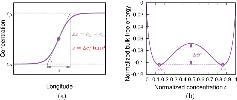
Figure 2: Definition of interface thickness for a 1D problem.

The damage-like order parameter $\displaystyle\xi$ is introduced to describe the damage state of the material, with a value of 1 when the material is unbroken and being 0 when it is fully broken. According to Bourdin et al. [22], the fracture free energy density is given by,

$$\psi_{\mathrm{R}}^{f}(\xi,\bm{\nabla}_{\!\!\mathrm{R}}\xi)=\mathcal{G}_{c}\left[\epsilon|\bm{\nabla}_{\!\!\mathrm{R}}\xi|^{2}+\frac{1}{4\epsilon}(1-\xi)^{2}\right].$$ (17)

Here, $\displaystyle\mathcal{G}_{c}$ is the critical energy release rate, and $\displaystyle\epsilon$ is a length scale which determines the width of the transition zone between the unbroken and the broken region.

The elastic energy $\displaystyle\psi^{e}_{\mathrm{R}}$ represents a stored energy of the elastic deformation. Although a crystal with anisotropic chemical properties will also show an anisotropy in mechanical properties, the quantitative relation is still unknown. For simplicity, for the undamaged region an isotropic neo-Hookean model is assumed

$$\psi_{\mathrm{R}}^{e0}(c_{\mathrm{R}},\mathbf{C})=J^{c}\left[\frac{K_{c}}{2}\left(J^{e}-1\right)^{2}+\frac{G_{c}}{2}\left(\bar{I}_{1}-3\right)\right],$$ (18)

in which $\displaystyle K_{c}$ and $\displaystyle G_{c}$ are phase-dependent elastic moduli which are expressed as

$$K_{c}=\mathrm{K}_{0}\left(c-\mathrm{c}_{\mathrm{in}}\right),\quad G_{c}=\mathrm{G}_{0}\left(c-\mathrm{c}_{\mathrm{in}}\right).$$ (19)

Here, K₀, G₀ and c_in are constants, and can be determined by a linear fitting of the measurements of the elastic moduli at different concentrations. For more details of an undamaged isotropic model we refer the reader to our previous work [23].

Following Schneider et al. [16] and Zuo et al. [18], we ignore the direct influence of diffusion on the crack propagation. That is, the chemical field will not directly lead to fracture, but through the stress field. Moreover, to account for the fact that cracks will not propagate under compressive volumetric stresses, the elastic free energy can be split into a positive part $\displaystyle\psi_{\mathrm{R}}^{e+}$ and a negative part $\displaystyle\psi_{\mathrm{R}}^{e-}$. The latter will not be involved in the coupling with the fracture. More specifically, the two parts take the form of

$$\displaystyle\psi_{\mathrm{R}}^{e+}(c_{\mathrm{R}},\mathbf{C})=J^{c}\left[\frac{K_{c}}{2}\left(J^{e+}-1\right)^{2}+\frac{G_{c}}{2}\left(\bar{I}_{1}-3\right)\right],$$ (20a)

$$\displaystyle\psi_{\mathrm{R}}^{e-}(c_{\mathrm{R}},J)=J^{c}\frac{K_{c}}{2}\left(J^{e-}-1\right)^{2},$$ (20b)

in which

$$\left\{\begin{array}[]{c c c c}J^{e+}=J^{e},&J^{e-}=1,&\mathrm{if}&J^{e}\geq 1;\\ J^{e+}=1,&J^{e-}=J^{e},&\mathrm{if}&J^{e}<1.\end{array}\right.$$ (21)

The elastic energy is defined as

$$\psi_{\mathrm{R}}^{e}(c_{\mathrm{R}},\mathbf{C},\xi)=(\xi^{2}+\eta)\psi_{\mathrm{R}}^{e+}+\psi_{\mathrm{R}}^{e-},$$ (22)

in which, $\displaystyle 0<\eta\ll 1$ is a constant introduced to prevent singularity inside the broken phase when $\displaystyle\xi=0$. This method has been successfully implemented in the works of Kuhn et al. [24, 25] and Schlüter et al. [26] with a careful choice of $\displaystyle\eta$.

2.3 Governing equations

In this model, there are three sets of field variables: a molar concentration $\displaystyle c_{\mathrm{R}}$, displacements $\displaystyle\bm{u}$, and a damage variable $\displaystyle\xi$. The variation of the total free energy can be expressed in terms of variations of those variables as

$$\delta\Psi=\int_{\mathrm{B}_{\mathrm{R}}}\mathbf{S}_{\mathrm{R}}:\delta\mathbf{E}\,\mathrm{dB}+\int_{\mathrm{B}_{\mathrm{R}}}\mu_{\mathrm{R}}\,\delta c_{\mathrm{R}}\,\mathrm{dB}+\int_{\mathrm{B}_{\mathrm{R}}}\zeta\,\delta\xi\,\mathrm{dB},$$ (23)

in which $\displaystyle\mathbf{S}_{\mathrm{R}}$ is the second Piola-Kirchhoff stress tensor, $\displaystyle\mu_{\mathrm{R}}$ is the chemical potential, $\displaystyle\zeta$ is the driving force for the fracture. $\displaystyle\Psi$ is defined as the free energy over the whole body as

$$\Psi=\int_{\mathrm{B}_{\mathrm{R}}}\psi_{\mathrm{R}}(c_{\mathrm{R}},\bm{\nabla}_{\!\!\mathrm{R}}c_{\mathrm{R}},\mathbf{C},\xi,\bm{\nabla}\xi)\,\mathrm{dB}.$$ (24)

With $\displaystyle\psi_{\mathrm{R}}$ defined in (11), the variation of $\displaystyle\Psi$ is given by

$$\displaystyle\delta\Psi \displaystyle=\int_{\mathrm{B}_{\mathrm{R}}}\left[\frac{\mathrm{d}\psi^{c}_{\mathrm{R}}}{\mathrm{d}c_{\mathrm{R}}}\delta c_{\mathrm{R}}+{\frac{\mathrm{d}\psi^{i}_{\mathrm{R}}}{\mathrm{d}\bm{\nabla}_{\!\mathrm{R}}c_{\mathrm{R}}}}\cdot\delta\bm{\nabla}_{\!\mathrm{R}}c_{\mathrm{R}}+\frac{\partial\psi^{e}_{\mathrm{R}}}{\partial c_{\mathrm{R}}}\delta c_{\mathrm{R}}+\frac{\partial\psi^{e}_{\mathrm{R}}}{\partial\mathbf{C}}:\delta\mathbf{C}\right.$$

$$\displaystyle\quad+\left.\frac{\partial\psi^{e}_{\mathrm{R}}}{\partial\xi}\delta\xi+\frac{\partial\psi^{f}_{\mathrm{R}}}{\partial\xi}\delta\xi+\frac{\partial\psi^{f}_{\mathrm{R}}}{\partial\bm{\nabla}\xi}\cdot\delta\bm{\nabla}\xi\right]\,\mathrm{dB}$$

$$\displaystyle=\int_{\mathrm{B}_{\mathrm{R}}}\left\{\left(\frac{\mathrm{d}\psi^{c}_{\mathrm{R}}}{\mathrm{d}c_{\mathrm{R}}}-\bm{\nabla}_{\!\mathrm{R}}\cdot\mathbf{K}\bm{\nabla}_{\!\mathrm{R}}c_{\mathrm{R}}+\frac{\partial\psi^{e}_{\mathrm{R}}}{\partial c_{\mathrm{R}}}\right)\delta c_{\mathrm{R}}+\bm{\nabla}_{\!\mathrm{R}}\cdot(\mathbf{K}\bm{\nabla}_{\!\mathrm{R}}c_{\mathrm{R}}\delta c_{\mathrm{R}})+\frac{2\partial\psi^{e}_{\mathrm{R}}}{\partial\mathbf{C}}:\delta\mathbf{E}\right.$$

$$\displaystyle\quad+\left[2\xi\psi^{e+}_{\mathrm{R}}\left.+\frac{\mathcal{G}_{c}}{2\epsilon}\left(\xi-1\right)-2\mathcal{G}_{c}\epsilon\Delta_{\mathrm{R}}\xi\right]\delta\xi+\bm{\nabla}_{\!\mathrm{R}}\cdot\left(\bm{\nabla}_{\!\mathrm{R}}\xi\delta\xi\right)\right\}\,\mathrm{dB}$$

$$\displaystyle=\displaystyle\int_{\mathrm{B}_{\mathrm{R}}}\left(\frac{\mathrm{d}\psi^{c}_{\mathrm{R}}}{\mathrm{d}c_{\mathrm{R}}}-\bm{\nabla}_{\!\mathrm{R}}\cdot\mathbf{K}\bm{\nabla}_{\!\mathrm{R}}c_{\mathrm{R}}+\frac{\partial\psi^{e}_{\mathrm{R}}}{\partial c_{\mathrm{R}}}\right)\delta c_{\mathrm{R}}\,\mathrm{dB}+\int_{\mathrm{B}_{\mathrm{R}}}\frac{2\partial\psi^{e}_{\mathrm{R}}}{\partial\mathbf{C}}:\delta\mathbf{E}\,\mathrm{dB}$$

$$\displaystyle\quad+\int_{\mathrm{B}_{\mathrm{R}}}\left[2\xi\psi^{e+}_{\mathrm{R}}+\frac{\mathcal{G}_{c}}{2\epsilon}\left(\xi-1\right)-2\mathcal{G}_{c}\epsilon\Delta_{\mathrm{R}}\xi\right]\delta\xi\,\mathrm{dB}$$

$$\displaystyle\quad+{\int_{\partial\mathrm{B}_{\mathrm{R}}}\mathbf{K}\bm{\nabla}_{\!\mathrm{R}}c_{\mathrm{R}}\cdot\mathbf{n}_{\mathrm{R}}\,\delta c_{\mathrm{R}}\,\mathrm{dS}}+\int_{\partial\mathrm{B}_{\mathrm{R}}}\bm{\nabla}_{\!\mathrm{R}}\xi\cdot\mathbf{n}_{\mathrm{R}}\,\delta\xi\,\mathrm{dS}.$$ (25)

Comparing (23) and (25), $\displaystyle\mathbf{S}_{\mathrm{R}}$, $\displaystyle\mu_{\mathrm{R}}$, $\displaystyle\zeta$ can be written as

$$\displaystyle\mathbf{S}_{\mathrm{R}}=\frac{2\partial\psi_{\mathrm{R}}}{\partial\mathbf{C}}=\left(\xi^{2}+\eta\right)\frac{2\partial\psi_{\mathrm{R}}^{e+}}{\partial\mathbf{C}}+\frac{2\partial\psi_{\mathrm{R}}^{e-}}{\partial\mathbf{C}},$$ (26a)

$$\displaystyle\mu_{\mathrm{R}}=\frac{\mathrm{d}\psi_{\mathrm{R}}^{c}}{\mathrm{d}c_{\mathrm{R}}}+\frac{\partial\psi_{\mathrm{R}}^{e}}{\partial c_{\mathrm{R}}}-\bm{\nabla}_{\!\!\mathrm{R}}\cdot\mathbf{K}\bm{\nabla}_{\!\!\mathrm{R}}c,$$ (26b)

$$\displaystyle\zeta=2\xi\psi_{\mathrm{R}}^{e+}-2\mathcal{G}_{c}\epsilon\Delta_{\!\mathrm{R}}\xi+\frac{\mathcal{G}_{c}}{2\epsilon}(\xi-1),$$ (26c)

with two boundary conditions $\displaystyle\mathbf{K}\bm{\nabla}_{\mathrm{R}}c_{\mathrm{R}}\cdot\mathbf{n}_{\mathrm{R}}=0$ and $\displaystyle\bm{\nabla}_{\mathrm{R}}\xi\cdot\mathbf{n}_{\mathrm{R}}=0$ to be fulfilled on the boundary surface in the reference configuration $\displaystyle\partial\mathrm{B}_{\mathrm{R}}$, in addition to the Dirichlet and Neumann boundary conditions from physical constraints and fluxes.

As for the governing equation of the mechanical part, we assume a quasi-static loading, thus ignoring the inertia terms. The governing equation for the local force balance in the body of the reference configuration B_R reads

$$\bm{\nabla}_{\!\!\mathrm{R}}\cdot\mathbf{P}_{\mathrm{R}}=\mathbf{0},$$ (27)

where $\displaystyle\mathbf{P}_{\mathrm{R}}$ is the first Piola-Kirchhoff stress, defined as

$$\mathbf{P}=\mathbf{F}\,\mathbf{S}_{\mathrm{R}}.$$ (28)

Molar concentration $\displaystyle c_{\mathrm{R}}$ is a conserved order parameter and subject to Cahn-Hilliard-type kinetics. In the authors’ previous paper [23], the species are assumed to be driven by a flux defined in the reference configuration, which leads to simplification in finite element implementation. In the present paper, a more physically based kinetics is employed, which defines the flux by the gradient of chemical potential at the current configuration. More specifically,

$$\frac{\partial c_{\mathrm{C}}}{\partial t}=-\bm{\nabla}_{\mathrm{\!\!C}}\cdot\bm{j}_{\mathrm{C}}$$ (29)

where the subscript C denotes quantities defined in the current configuration.

In the body B_C, the Cahn-Hilliard-type diffusion applies in the virgin state, while in the damaged region no diffusion is considered. It leads to

$$\bm{j}_{\mathrm{C}}=-\xi^{2}\bm{M}_{c}\bm{\nabla}\mu_{\mathrm{R}}\quad\mathrm{in}\quad\mathrm{B}_{\mathrm{C}},\\$$ (30)

where $\displaystyle\bm{M}_{c}$ is a mobility tensor defined as

$$\bm{M}_{c}=c(1-c)\left[\begin{array}[]{c c c}\mathrm{M}_{x}&&\\ &\mathrm{M}_{y}&\\ &&\mathrm{M}_{z}\end{array}\right]=c(1-c)\mathbf{M},$$ (31)

with $\displaystyle c(1-c)$ representing a degenerated mobility towards $\displaystyle c=0$ and $\displaystyle c=1$. On the boundary surface $\displaystyle\partial\mathrm{B}_{\mathrm{C}}$ and the surface of a newly created crack $\displaystyle\Gamma_{f}$, the flux is dependent on the electrochemical reaction, which follows a phenomenological Butler-Volmer equation. More details will follow in sections 3.1 and 3.2. Therefore, the flux is given as

$$\bm{j}_{\mathrm{C}}\cdot\mathbf{n}_{\mathrm{C}}=-\hat{j\,}_{s}\quad\mathrm{on}\quad\partial\mathrm{B}_{\mathrm{C}}\cup\Gamma_{f}.$$ (32)

Based on density functional theory calculations, Rohrer et al. [13] have concluded that the anisotropy of mobility is a consequence of orientation-dependent interface energies, and that high-energy interfaces are more mobile than low-energy interfaces. By recalling (16), it can be concluded that a higher $\displaystyle\kappa$ leads to a larger $\displaystyle M$. For simplicity, a proportional relation is assumed, that is, $\displaystyle\mathrm{M}_{x}:\mathrm{M}_{y}:\mathrm{M}_{z}=\kappa_{x}:\kappa_{y}:\kappa_{z}$. The chemical potential $\displaystyle\mu_{\mathrm{R}}$ expresses the free energy change for adding/subtracting one mole lithium into/out of the system, thus being the same for any configurations. The subscript R only indicates the fact that it is calculated by quantities in the reference configuration. Given the condition that the total mass should be conserved in different configurations,

$$\int_{\mathrm{B}_{\mathrm{C}}}\frac{\partial c_{\mathrm{C}}}{\partial t}\,\mathrm{d}\mathrm{B}=\int_{\mathrm{B}_{\mathrm{R}}}\frac{\partial c_{\mathrm{R}}}{\partial t}\,\mathrm{d}\mathrm{B},$$ (33)

equation (29) can be pulled back straightforwardly to the reference configuration as

$$\frac{\partial c_{\mathrm{R}}}{\partial t}=\bm{\nabla}_{\!\!\mathrm{R}}\cdot\left[\xi^{2}c(1-c)J\mathbf{F}^{-1}\mathbf{M}\mathbf{F}^{-\mathrm{T}}\bm{\nabla}_{\!\!\mathrm{R}}\mu_{\mathrm{R}}\right]\quad\mathrm{in}\quad\mathrm{B}_{\mathrm{R}}.$$ (34)

For later discussion, a dimensionless activity $\displaystyle a$ is introduced

$$\mathrm{RT}\ln a=\mu_{\mathrm{R}},$$ (35)

and an activity coefficient $\displaystyle\gamma$ as a ratio $\displaystyle\gamma=a/c$. Note that, when $\displaystyle a=c$ and thus $\displaystyle\gamma=1$, this model degenerates to an ideal dilute model.

As for a non-conserved order parameter $\displaystyle\xi$, the evolution equation follows an Allen-Cahn-type equation

$$\frac{\partial\xi}{\partial t}=-\mathrm{M}_{\xi}\zeta=-\mathrm{M}_{\xi}\left[2\xi\psi_{\mathrm{R}}^{e+}-2\mathcal{G}_{c}\epsilon\Delta_{\!\mathrm{R}}\xi+\frac{\mathcal{G}_{c}}{2\epsilon}(\xi-1)\right]$$ (36)

with M_ξ as the mobility for the evolution of $\displaystyle\xi$. Following Miehe et al. [27, 28] and Borden et al. [29], to mimic the irreversibility of the crack, a strain-history field $\displaystyle\mathcal{H}_{\mathrm{R}}$ is introduced as a substitution of $\displaystyle\psi_{\mathrm{R}}^{e+}$, which satisfies the Kuhn-Tucker conditions

$$\mathcal{H}_{\mathrm{R}}\geq\psi_{\mathrm{R}}^{e+},\quad\dot{\mathcal{H}_{\mathrm{R}}}\geq 0,\quad\dot{\mathcal{H}_{\mathrm{R}}}\left(\psi_{\mathrm{R}}^{e+}-\mathcal{H}_{\mathrm{R}}\right)=0.$$ (37)

The evolution for $\displaystyle\xi$ then reads

$$\frac{\partial\xi}{\partial t}=-\mathrm{M}_{\xi}\left[2\xi\mathcal{H}_{\mathrm{R}}-2\mathcal{G}_{c}\epsilon\Delta_{\!\mathrm{R}}\xi+\frac{\mathcal{G}_{c}}{2\epsilon}(\xi-1)\right].$$ (38)

In summary, the governing equations for three field variables $\displaystyle\bm{u}$, $\displaystyle c$ and $\displaystyle\xi$ are given in (27), (34) and (38), respectively.

3 Modeling of electrochemical reaction

3.1 Reaction on particle surfaces

On the particle surface, a Faradaic reaction

$$\mathrm{Li}^{+}+e^{-}\rightleftharpoons\mathrm{Li}$$ (39)

takes place, during which a Li-ion consumes an electron, as shown in Figure 3. The resultant neutral Lithium inserts into the host material.

Figure 3: Illustration of the electrochemical reaction on the surface

The rate of the reaction is described by a phenomenological Butler-Volmer (BV) equation,

$$\hat{j\,}_{s}=\mathrm{c}_{s}\mathrm{R}_{\mathrm{BV}}=\mathrm{c}_{s}\frac{a_{+}^{1-\beta}a^{\beta}}{\tau_{0}\gamma_{\mathrm{A}}}\left[\exp\left(-\beta\frac{\mathrm{F}\eta^{s}_{\mathrm{R}}}{\mathrm{RT}}\right)-\exp\left(\left(1-\beta\right)\frac{\mathrm{F}\eta^{s}_{\mathrm{R}}}{\mathrm{RT}}\right)\right],$$ (40)

in which c_s with the unit of $\displaystyle\text{\,}\mathrm{mol}\text{\,}{\mathrm{m}}^{-2}$ is the molar concentration of intercalation sites on the surface, R_BV is the reaction rate in unit $\displaystyle\text{\,}{\mathrm{s}}^{-1}$. Moreover, $\displaystyle\tau_{0}$ is the mean time for a single reaction step, which will be set differently to mimic a slow or fast reaction process in the simulation. The parameter $\displaystyle\gamma_{\mathrm{A}}$ denotes the chemical activity coefficient of the activated state, which is taken as $\displaystyle(1-c)^{-1}$, while $\displaystyle\beta$ is a symmetry factor for a forward and backward reaction indicated in (39) and is set to be $\displaystyle 0.5$. The Faraday constant F describes the amount of electric charge of one mole electrons. For more details on coefficients of this model, one can refer to the work of Bai et al. [2] and Dargaville et al. [3]. The definition of $\displaystyle a$ has been introduced in (35). The parameters $\displaystyle a_{+}$ and $\displaystyle a$ are activities of Li⁺ and Li, respectively. Since Li⁺ diffuses in the electrolyte much faster than Li diffuses in the electrode [2], $\displaystyle a_{+}$ is set to be unity for simplicity. For a similar reason, the activity of electrons $\displaystyle a_{-}$ is also set to be 1. The surface overpotential $\displaystyle\eta^{s}_{\mathrm{R}}$ is defined as the electrostatic potential of the working electrode relative to a reference electrode of the same kind placed in the solution adjacent to the surface of the working electrode. It can be expressed in terms of the electrochemical potentials as

$$\mathrm{F}\eta^{s}_{\mathrm{R}}=\mu_{\mathrm{Li}}-\mu_{\mathrm{Li}^{+}}-\mu_{e^{-}},$$ (41)

where $\displaystyle\mu_{\mathrm{Li}}$, $\displaystyle\mu_{\mathrm{Li}^{+}}$, $\displaystyle\mu_{e^{-}}$ are electrochemical potential of Li, Li⁺ and $\displaystyle e^{-}$, respectively, and which are expressed as

$$\displaystyle\mu_{\mathrm{Li}}=\mathrm{RT}\ln a=\mu_{\mathrm{R}},$$ (42)

$$\displaystyle\mu_{\mathrm{Li}^{+}}=\mathrm{RT}\ln a_{+}+\mathrm{F}\phi_{e}=\mathrm{F}\phi,$$ (43)

$$\displaystyle\mu_{e^{-}}=\mathrm{RT}\ln a_{-}-\mathrm{F}\phi=-\mathrm{F}\phi_{e}.$$ (44)

Here, $\displaystyle\phi_{e}$ denotes the electrostatic potential of the electrode, and $\displaystyle\phi$ represents that of the electrolyte. Insertion of the last three equations into the surface overpotential given in (41) leads to

$$\mathrm{F}\eta^{s}_{\mathrm{R}}=\mu_{\mathrm{R}}+\mathrm{F}\left(\phi_{e}-\phi\right)=\mu_{\mathrm{R}}+\mathrm{F}\mathbb{\Delta}\phi,$$ (45)

where $\displaystyle\mathbb{\Delta}\phi=\phi_{e}-\phi$ is the voltage drop across the electrode/electrolyte interface. As mentioned, the subscript R in $\displaystyle\eta$ is only to indicate that it is expressed by quantities in the reference configuration and is independent from the chosen configuration. On the other hand, the flux $\displaystyle\hat{j\,}_{s}$ is flow rate per unit area and is dependent on the configuration. However, this dependence is fully described in the parameter c_s. Therefore (40) is valid for both configurations, with the corresponding c_s. The same applies for the next section, where the reaction on the newly created crack surfaces is discussed.

By substituting (12), (26b) into (45), the normalized overpotential can be expressed as

$$\eta^{s}=\frac{\mathrm{F}\eta^{s}_{\mathrm{R}}}{\mathrm{RT}}=\ln\frac{c}{1-c}+\chi(1-2c)+\mu^{e}-\bm{\nabla}\cdot\mathbf{K}^{\ast}\bm{\nabla}c+\mathbb{\Delta}\phi^{\ast},$$ (46)

where $\displaystyle\mu^{e}=(1/\mathrm{RT})\partial\psi^{e}_{\mathrm{R}}/\partial c_{\mathrm{R}}$ is the normalized elastic chemical potential, $\displaystyle\mathbb{\Delta}\phi^{\ast}=\mathrm{F}\mathbb{\Delta}\phi/\left(\mathrm{RT}\right)$, $\displaystyle\mathbf{K}^{\ast}=\mathbf{K}/\left(\mathrm{RTL}_{0}^{2}\right)$, and $\displaystyle\bm{\nabla}=\mathrm{L}_{0}\bm{\nabla}_{\mathrm{R}}$. Here L₀ is a characteristic length which is introduced for normalization of the model discussed in Section 4.1

Note that, insertion of Li takes place on the surface for $\displaystyle\eta^{s}<0$, while extraction of Li happens for $\displaystyle\eta^{s}>0$. Thus, by choosing different voltage drop $\displaystyle\mathbb{\Delta}\phi^{\ast}$, the reaction can be controlled as forward and backward. In particular, when the interfacial and elastic chemical potential is disregarded, $\displaystyle\eta^{s}=\mu^{c}+\mathbb{\Delta}\phi^{\ast}$. As shown in Figure 4(a), when $\displaystyle\mathbb{\Delta}\phi^{\ast}$ is negative and large enough, the system will absorb Li until $\displaystyle c=c_{1}$ is reached. On the contrary, as shown in Figure 4(c), when $\displaystyle\mathbb{\Delta}\phi^{\ast}$ is positive and large enough, Li will be deintercalated from the system until $\displaystyle c=c_{5}$. However, when $\displaystyle-\mathbb{\Delta}\phi^{\ast}$ stays between two spinodal points, as shown in Figure 4(b), it is highly probable that both insertion and extraction will take place at the same time towards $\displaystyle c=c_{2}$ and $\displaystyle c=c_{3}$, since the whole system is unstable due to spinodal decomposition. Notice that $\displaystyle c_{2}$ and $\displaystyle c_{3}$ can be different from the concentrations in two phases $\displaystyle c_{\alpha}$ and $\displaystyle c_{\beta}$, which are the results of the spinodal decomposition. The values of $\displaystyle c_{2}$ and $\displaystyle c_{3}$ depend not only on the chemical state of the material, but also on the applied voltage potential drop $\displaystyle\mathbb{\Delta}\phi^{\ast}$. The reaction on the surface will automatically constrain the concentration in a way that the concentration will stay in the range from 0 to 1.

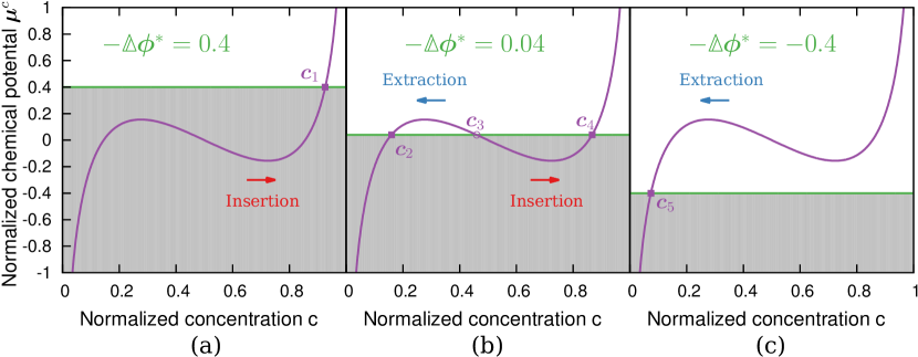
Figure 4: Insertion/extraction of Li under different normalized voltage drop $\displaystyle\mathbb{\Delta}\phi^{\ast}=\mathrm{F}\mathbb{\Delta}\phi/\left(\mathrm{RT}\right)$. The chemical potential $\displaystyle\mu^{c}=\ln c-\ln(1-c)+2.5\left(1-2c\right).$

Substitution of (46) into (40) leads to

$$\hat{j\,}_{s}=\frac{\mathrm{c}_{s}}{\tau_{0}}\left(1-c\right)\exp\left(-\frac{1}{2}\mathbb{\Delta}\phi^{\ast}\right)-\frac{\mathrm{c}_{s}}{\tau_{0}}\,c\exp\left[\chi\left(1-2c\right)+\mu^{e}-\bm{\nabla}\cdot\mathbf{K}^{\ast}\bm{\nabla}c+\frac{1}{2}\mathbb{\Delta}\phi^{\ast}\right].$$ (47)

3.2 Reaction on crack surfaces

In the framework of phase-field fracture models, the crack interface can be tracked through $\displaystyle\xi(\xi-1)\neq 0$ or $\displaystyle\bm{\nabla}\xi\neq 0$. Therefore, the boundary flux can be weighted by functions containing either or both of these two terms, in order to consider the reaction at the crack interface.

Denote the idealized crack surface by $\displaystyle\Gamma_{f}$ (one crack will create two surfaces facing towards each other), and by $\displaystyle\Gamma^{\prime}_{f}$ the level surface in the phase-field model for a constant $\displaystyle\xi$. The damage variable gradient $\displaystyle\bm{\nabla}\xi$ remains thus perpendicular to $\displaystyle\Gamma^{\prime}_{f}$. Introduce a vector $\displaystyle\bm{s}$, which lies parallel to the damage variable gradient $\displaystyle\bm{\nabla}\xi$. The flux on the crack surface can hence be approximated as the flux average across the interface

$$\int_{\Gamma_{f}}\hat{j\,}_{s}\,\mathrm{d}\Gamma\approx\frac{1}{\epsilon}\int_{s}\int_{\Gamma^{\prime}_{f}}g(\xi,\bm{\nabla}\xi)\hat{j\,}_{s}\,\mathrm{d}\Gamma^{\prime}\mathrm{d}s\approx\frac{1}{\epsilon}\int_{\mathrm{B}}g(\xi,\bm{\nabla}\xi)\hat{j\,}_{s}\,\mathrm{dB},$$ (48)

in which $\displaystyle\epsilon$ is a length parameter and related to the interface thickness. The weight function $\displaystyle g(\xi)$ contains either $\displaystyle\xi(\xi-1)$ or $\displaystyle\bm{\nabla}\xi$ as a factor. If the flux is kept constant across the interface, or varies very little along the direction of $\displaystyle\bm{\nabla}\xi$, we can observe the following relation

$$\frac{1}{\epsilon}\int_{s}\int_{\Gamma^{\prime}_{f}}g(\xi,\bm{\nabla}\xi)\hat{j\,}_{s}\,\mathrm{d}\Gamma^{\prime}\mathrm{d}s\approx\frac{1}{\epsilon}\int_{s}g(\xi,\bm{\nabla}\xi)\,\mathrm{d}s\int_{\Gamma^{\prime}}\hat{j\,}_{s}\mathrm{d}\Gamma^{\prime}.$$ (49)

It follows that the approximation of (48) is valid, if

$$\frac{1}{\epsilon}\int_{s}g(\xi,\bm{\nabla}\xi)\,\mathrm{d}s=1.$$ (50)

It should be commented that there will be several factors that can influence the accuracy of the approximation.

• The phase-field approximation of the cracked phase interface will determine the choice of $\displaystyle g(\xi)$. Usually $\displaystyle g(\xi)$ is chosen based on an uncoupled model for simplicity. However, when the mechanical stresses come into play, the $\displaystyle\xi$ profile can be different. The error can be even larger when $\displaystyle\xi(\xi-1)$ is used as its weighting term, since $\displaystyle\xi$ might not be 0 and 1 in two homogeneous phases, depending on the boundary condition given (the reader is referred to [29] for more details). Therefore $\displaystyle g(\xi)$ needs to be modified accordingly, when the influence of stresses is not negligible;

• The flux can vary strongly across the phase interface, especially when the diffusion is so slow that the concentration varies greatly along the direction of $\displaystyle\bm{\nabla}\xi$, making electrochemical reaction on/in the interface highly fluctuating in a small range. In these cases the equation (49) may not be accurate enough. One can, for instance, increase the polynomial order of $\displaystyle g(\xi)$, so that the fluctuation of the reaction will become negligible compared to $\displaystyle g(\xi)$.

As a simple case, we set $\displaystyle g(\xi)=\mathrm{A}\xi^{2}(1-\xi)^{2}$ with A being a coefficient to be determined. To this end, firstly, the profile of $\displaystyle\xi(x)$ across the interface on one side can be obtained by solving the following uncoupled 1D problem at equilibrium

$$\left\{\begin{array}[]{l c r}0=2\mathcal{G}_{c}\epsilon\xi^{\prime\prime}+\frac{1}{2}\frac{\mathcal{G}_{c}}{\epsilon}\left(s-1\right)&\mathrm{for}&0<x\leq\mathrm{L},\\ \xi|_{x=0}=0,&&\\ \xi^{\prime}|_{x=\mathrm{L}}=0.&&\end{array}\right.$$ (51)

The solution reads

$$\xi(x)=1-\cosh\left(\frac{x}{2\epsilon}\right)+\coth\left(\frac{\mathrm{L}}{2\epsilon}\right)\sinh\left(\frac{x}{2\epsilon}\right)=1+\sinh^{-1}\left(\frac{\mathrm{L}}{2\epsilon}\right)\sinh\left(\frac{x-\mathrm{L}}{2\epsilon}\right).$$ (52)

Inserting (52) into $\displaystyle g(\xi)$ and integrating over the whole length L, one has

$$\displaystyle 1 \displaystyle=\frac{1}{\epsilon}\mathrm{A}\int_{0}^{\mathrm{L}}\xi^{2}\left(1-\xi\right)^{2}\,\mathrm{d}x$$

$$\displaystyle=\frac{1}{\epsilon}\mathrm{A}\int_{0}^{\mathrm{L}}\left[1+\sinh^{-1}\left(\frac{\mathrm{L}}{2\epsilon}\right)\sinh\left(\frac{x-\mathrm{L}}{2\epsilon}\right)\right]^{2}\left[-\sinh^{-1}\left(\frac{\mathrm{L}}{2\epsilon}\right)\sinh\left(\frac{x-\mathrm{L}}{2\epsilon}\right)\right]^{2}\,\mathrm{d}x$$

$$\displaystyle\approx\frac{1}{\epsilon}\mathrm{A}\cdot\frac{1}{6}\epsilon=\frac{\mathrm{A}}{6},$$ (53)

which gives A$\displaystyle=6$ and $\displaystyle g(\xi)=6\xi^{2}(1-\xi)^{2}$. The evolution for the concentration can then be expanded from (34) as

$$\frac{\partial c_{\mathrm{R}}}{\partial t}=\bm{\nabla}_{\!\!\mathrm{R}}\cdot\left[\xi^{2}c(1-c)J\mathbf{F}^{-1}\mathbf{M}\mathbf{F}^{-\mathrm{T}}\bm{\nabla}_{\!\!\mathrm{R}}\mu_{\mathrm{R}}\right]+\frac{6}{\epsilon}\xi^{2}\left(1-\xi\right)^{2}\hat{j\,}_{s},$$ (54)

in which $\displaystyle\hat{j\,}_{s}$ is given in (47) to account for the flux due to electrochemical reaction.

4 Numerical treatment

4.1 Normalization

For the convenience of finite element implementation, the model presented above is normalized first. Introduce a dimensionless form of space and time as

$$\bar{\mathbf{X}}=\frac{\mathbf{X}}{\mathrm{L}_{0}},\quad\bar{t}=\frac{\mathrm{D}}{\mathrm{L}_{0}^{2}}\,t.$$ (55)

in which L₀ is a characteristic length scale, which is identical in the three directions, and D is a diffusion coefficient of one direction. Energy density is scaled by RTc_max, and the other quantities can be normalized accordingly as

$$\psi=\frac{\psi_{\mathrm{R}}}{\mathrm{RT}\mathrm{c}_{\mathrm{max}}},\quad\mu=\frac{\mu_{\mathrm{R}}}{\mathrm{RT}},\quad\mathbf{j}=\frac{\mathrm{L}_{0}}{\mathrm{D}\mathrm{c}_{\mathrm{max}}}\,\mathbf{j}_{\mathrm{R}},\quad\mathbf{S}=\frac{\mathbf{S}_{\mathrm{R}}}{\mathrm{RT}\mathrm{c}_{\mathrm{max}}},\quad\mathcal{H}=\frac{\mathcal{H}_{\mathrm{R}}}{\mathrm{RTc}_{\mathrm{max}}}.$$ (56)

For the fracture model, the normalized fracture length scale, energy release rate and the mobility are

$$\epsilon^{\ast}=\frac{\epsilon}{\mathrm{L}_{0}},\quad\mathcal{G}_{c}^{\ast}=\frac{\mathcal{G}_{c}}{\mathrm{L}_{0}\mathrm{RTc}_{\mathrm{max}}},\quad\mathrm{M}_{\xi}^{\ast}=\frac{\mathrm{M}_{\xi}\mathrm{L}_{0}^{2}\mathrm{RTc}_{\mathrm{max}}}{\mathrm{D}}$$ (57)

For the reaction, the surface site concentration c_s and the single reaction time step $\displaystyle\tau_{0}$ is

$$\mathrm{c}_{s}^{\ast}=\frac{\mathrm{c}_{s}}{\mathrm{c}_{\mathrm{max}}\mathrm{L}_{0}},\quad\tau_{0}^{\ast}=\frac{\mathrm{D}}{\mathrm{L}_{0}^{2}}\tau_{0}$$ (58)

Thus the normalized governing equations can be summarized as:

$$\left\{\begin{array}[]{l c l l l}\bm{\nabla}\cdot\mathbf{P}=\mathbf{0}&\mathrm{in}&\mathrm{B}&\times&\left[0,\bar{\mathcal{T}}\right],\\ \dot{c}=\bm{\nabla}\cdot\left[\xi^{2}c(1-c)J\mathbf{F}^{-1}\mathbf{M}^{\ast}\mathbf{F}^{-\mathrm{T}}\bm{\nabla}\mu\right]+\frac{6}{\epsilon^{\ast}}\xi^{2}\left(1-\xi\right)^{2}\bar{\hat{j\,}}_{s},&\mathrm{in}&\mathrm{B}&\times&\left[0,\bar{\mathcal{T}}\right],\\ \dot{\xi}=-M_{\xi}^{\ast}\left[2\xi\mathcal{H}-2\mathcal{G}_{c}^{\ast}\epsilon^{\ast}\Delta\xi+\frac{\mathcal{G}_{c}^{\ast}}{2\epsilon^{\ast}}\left(\xi-1\right)\right],&\mathrm{in}&\mathrm{B}&\times&\left[0,\bar{\mathcal{T}}\right],\\ \bar{\mathbf{u}}=\hat{\bar{\mathbf{u}}}&\mathrm{on}&\mathrm{S}_{\bar{\mathbf{u}}}&\times&\left[0,\bar{\mathcal{T}}\right],\\ \mathbf{P}\cdot\mathbf{n}=\hat{\bar{\mathbf{t}}}&\mathrm{on}&\mathrm{S}_{\bar{\mathbf{t}}}&\times&\left[0,\bar{\mathcal{T}}\right],\\ \mathbf{j}\cdot\mathbf{n}=-\bar{\hat{j\,}}_{s}&\mathrm{on}&\partial\mathrm{B}&\times&\left[0,\bar{\mathcal{T}}\right],\\ \mathbf{K}\bm{\nabla}c\cdot\mathbf{n}=0&\mathrm{on}&\partial\mathrm{B}&\times&\left[0,\bar{\mathcal{T}}\right],\\ \bm{\nabla}\xi\cdot\mathbf{n}=0&\mathrm{on}&\partial\mathrm{B}&\times&\left[0,\bar{\mathcal{T}}\right],\\ c\left(\bar{\mathbf{X}},0\right)=c_{0}\left(\bar{\mathbf{X}}\right)&\mathrm{in}&\mathrm{B},&&\\ \xi\left(\bar{\mathbf{X}},0\right)=0&\mathrm{on}&\Gamma_{f},&&\\ \xi\left(\bar{\mathbf{X}},0\right)=1&\mathrm{in}&\mathrm{B}\backslash\Gamma_{f},&&\end{array}\right.$$ (59)

with $\displaystyle\bar{\hat{j\,}}_{s}$ defined as

$$\bar{\hat{j\,}}_{s}=\frac{\mathrm{c}_{s}^{\ast}}{\tau_{0}^{\ast}}\left(1-c\right)\exp\left(-\frac{1}{2}\mathbb{\Delta}\phi^{\ast}\right)-\frac{\mathrm{c}_{s}^{\ast}}{\tau_{0}^{\ast}}\,c\exp\left[\chi\left(1-2c\right)+\mu^{e}-\bm{\nabla}\cdot\mathbf{K}^{\ast}\bm{\nabla}c+\frac{1}{2}\mathbb{\Delta}\phi^{\ast}\right]$$ (60)

4.2 Implementation details

This model is implemented by using the finite element program FEAP [30] with Non-Uniform Rational B-Splines (NURBS) as shape functions for the spatial discretization, which allow for a straightforward treatment of the fourth-order Cahn-Hilliard equation. The displacements $\displaystyle\bm{u}$, the concentration $\displaystyle c$ and the order parameter $\displaystyle\xi$ are nodal degrees of freedom. In addition, to deal with the additional boundary condition $\displaystyle\mathbf{K}\bm{\nabla}c\cdot\mathbf{n}=0$ arising along with the Cahn-Hilliard equation, a Lagrange multiplier $\displaystyle\lambda$ is introduced as an additional degree of freedom for each node. For more details about $\displaystyle\lambda$ the reader is referred to our previous work [23]. A backward Euler method is employed for the time integration, and Newton-Raphson iteration scheme is used for the nonlinear system of equations at each time step.

The above mentioned 6 field variables are interpolated under an isoparametric/isogeometric concept as

$$\bm{u}=N^{\mathrm{I}}\bm{u}^{\mathrm{I}},\quad c=N^{\mathrm{I}}c^{\mathrm{I}},\quad\xi=N^{\mathrm{I}}\xi^{\mathrm{I}},\quad\lambda=N^{\mathrm{I}}\lambda^{\mathrm{I}},$$ (61)

where $\displaystyle\left(\cdot\right)^{\mathrm{I}}$ is the value at the I-th control point, and $\displaystyle N^{\mathrm{I}}$ is the NURBS shape function associated with the I-th control point. The repeated I invokes the Einstein summation. The gradient terms are thus given by

$$\delta\mathbf{\underline{E}}=\mathbf{B}_{\bm{u}}^{\mathrm{I}}\delta\bm{u}^{\mathrm{I}},\quad\bm{\nabla}c=\mathbf{B}_{c}^{\mathrm{I}},\quad\bm{\nabla}\xi=\mathbf{B}_{\xi}^{\mathrm{I}},\quad\bm{\nabla}\lambda=\mathbf{B}_{\lambda}^{\mathrm{I}},$$ (62)

where $\displaystyle\mathbf{\underline{E}}$ is the Green-Lagrangian strain tensor in Voigt notation,

$$\mathbf{B}_{c}^{\mathrm{I}}=\mathbf{B}_{\xi}^{\mathrm{I}}=\mathbf{B}_{\lambda}^{\mathrm{I}}=\bm{\nabla}N^{\mathrm{I}}=\left[\begin{array}[]{c c c}N^{\mathrm{I}}_{,1}&N^{\mathrm{I}}_{,2}&N^{\mathrm{I}}_{,3}\end{array}\right]^{\mathrm{T}},$$ (63)

and

$$\mathbf{B}_{\bm{u}}^{\mathrm{I}}=\left[\begin{array}[]{c c c}F_{11}N^{\mathrm{I}}_{,1}&F_{21}N^{\mathrm{I}}_{,1}&F_{31}N^{\mathrm{I}}_{,1}\\ F_{12}N^{\mathrm{I}}_{,2}&F_{22}N^{\mathrm{I}}_{,2}&F_{32}N^{\mathrm{I}}_{,2}\\ F_{13}N^{\mathrm{I}}_{,3}&F_{23}N^{\mathrm{I}}_{,3}&F_{33}N^{\mathrm{I}}_{,3}\\ F_{11}N^{\mathrm{I}}_{,2}+F_{12}N^{\mathrm{I}}_{,1}&F_{21}N^{\mathrm{I}}_{,2}+F_{12}N^{\mathrm{I}}_{,1}&F_{31}N^{\mathrm{I}}_{,2}+F_{12}N^{\mathrm{I}}_{,1}\\ F_{12}N^{\mathrm{I}}_{,3}+F_{13}N^{\mathrm{I}}_{,2}&F_{22}N^{\mathrm{I}}_{,3}+F_{13}N^{\mathrm{I}}_{,2}&F_{32}N^{\mathrm{I}}_{,3}+F_{13}N^{\mathrm{I}}_{,2}\\ F_{13}N^{\mathrm{I}}_{,1}+F_{11}N^{\mathrm{I}}_{,3}&F_{23}N^{\mathrm{I}}_{,1}+F_{11}N^{\mathrm{I}}_{,3}&F_{33}N^{\mathrm{I}}_{,1}+F_{11}N^{\mathrm{I}}_{,3}\\ \end{array}\right].$$ (64)

Here, $\displaystyle N^{\mathrm{I}}_{,i}$ denotes $\displaystyle\partial N^{\mathrm{I}}/\partial X_{i}$, and $\displaystyle F_{ij}$ are the components of the deformation gradient $\displaystyle\mathbf{F}$.

Thus the discretized weak statement of (59) reads

$$\delta\Pi=(\delta\mathbf{u}^{\mathrm{I}})^{\mathrm{T}}\,\mathbf{R}^{\mathrm{I}}_{u}+\delta c^{\mathrm{I}}\,\mathrm{R}^{\mathrm{I}}_{c}+\delta\xi^{\mathrm{I}}\,\mathrm{R}^{\mathrm{I}}_{\xi}+\delta\lambda^{\mathrm{I}}\,\mathrm{R}^{\mathrm{I}}_{\lambda}=0,$$ (65)

in which the residuals are

$$\displaystyle\mathbf{R}^{\mathrm{I}}_{u} \displaystyle=\displaystyle-\int_{\mathrm{B}}(\mathbf{B}^{\mathrm{I}}_{u})^{\mathrm{T}}\left[\left(\xi^{2}+\eta\right)\frac{\partial\psi^{e+}}{\partial\mathbf{\underline{E}}}+\frac{\partial\psi^{e-}}{\partial\mathbf{\underline{E}}}\right]\,\mathrm{dB},$$ (66a)

$$\displaystyle\mathrm{R}^{\mathrm{I}}_{c} \displaystyle=\int_{\mathrm{B}}\dot{c}\,N^{\mathrm{I}}\,\mathrm{dB}+\int_{\mathrm{B}}\xi^{2}\left[1-2\chi c\left(1-c\right)\right]J\,(\bm{\nabla}c\cdot\mathbf{F}^{-1}\mathbf{M}^{\ast}\mathbf{F}^{-\mathrm{T}}\bm{\nabla}N^{\mathrm{I}})\,\mathrm{dB}$$

$$\displaystyle+\int_{\mathrm{B}}\xi^{2}c\left(1-c\right)J\,(\bm{\nabla}\mu^{e}\cdot\mathbf{F}^{-1}\mathbf{M}^{\ast}\mathbf{F}^{-\mathrm{T}}\bm{\nabla}N^{\mathrm{I}})\,\mathrm{dB}$$

$$\displaystyle+\int_{\mathrm{B}}2\xi c\left(1-c\right)J(\bm{\nabla}\cdot\mathbf{K}^{\ast}\bm{\nabla}c)\,(\bm{\nabla}\xi\cdot\mathbf{F}^{-1}\mathbf{M}^{\ast}\mathbf{F}^{-\mathrm{T}}\bm{\nabla}N^{\mathrm{I}})\,\mathrm{dB}$$

$$\displaystyle+\int_{\mathrm{B}}\xi^{2}\left(1-2c\right)J\,(\bm{\nabla}\cdot\mathbf{K}^{\ast}\bm{\nabla}c)\,(\bm{\nabla}c\cdot\mathbf{F}^{-1}\mathbf{M}^{\ast}\mathbf{F}^{-\mathrm{T}}\bm{\nabla}N^{\mathrm{I}})\,\mathrm{dB}$$

$$\displaystyle+\int_{\mathrm{B}}\xi^{2}c\left(1-c\right)(\bm{\nabla}\cdot\mathbf{K}^{\ast}\bm{\nabla}c)\,(\bm{\nabla}J\cdot\mathbf{F}^{-1}\mathbf{M}^{\ast}\mathbf{F}^{-\mathrm{T}}\bm{\nabla}N^{-1})\,\mathrm{dB}$$

$$\displaystyle+\int_{\mathrm{B}}\xi^{2}c\left(1-c\right)\,(\bm{\nabla}\cdot\mathbf{K}^{\ast}\bm{\nabla}c)\,\Delta N^{\mathrm{I}}\,\mathrm{dB}$$

$$\displaystyle+\int_{\mathrm{B}}\xi^{2}c\left(1-c\right)J\,(\bm{\nabla}\cdot\mathbf{K}^{\ast}\bm{\nabla}c)\,\left[\left(\bm{\nabla}\cdot\mathbf{F}^{-1}\mathbf{M}^{\ast}\mathbf{F}^{-\mathrm{T}}\right)\cdot\bm{\nabla}N^{\mathrm{I}}\right]\,\mathrm{dB}$$

$$\displaystyle+\int_{\mathrm{B}}\xi^{2}c\left(1-c\right)J\,(\bm{\nabla}\cdot\mathbf{K}^{\ast}\bm{\nabla}c)\,\left(\mathbf{F}^{-1}\mathbf{M}^{\ast}\mathbf{F}^{-\mathrm{T}}:\bm{\nabla}\bm{\nabla}N^{\mathrm{I}}\right)\,\mathrm{dB}$$

$$\displaystyle-\int_{\mathrm{B}}\frac{6\xi^{2}\left(1-\xi\right)^{2}}{\epsilon^{\ast}}\hat{j\,}_{s}N^{\mathrm{I}}\,\mathrm{dB}-\int_{\partial\mathrm{B}}\hat{j\,}^{s}\,N^{\mathrm{I}}\,\mathrm{dS}$$

$$\displaystyle+\int_{\mathrm{B}}\bm{\nabla}\lambda\cdot\mathbf{K}^{\ast}\bm{\nabla}N^{\mathrm{I}}\,\mathrm{dB}+\int_{\mathrm{B}}\lambda\,\bm{\nabla}\cdot\mathbf{K}^{\ast}\bm{\nabla}N^{\mathrm{I}}\,\mathrm{dB},$$ (66b)

$$\displaystyle\mathrm{R}^{\mathrm{I}}_{\xi} \displaystyle=\int_{\mathrm{B}}\dot{\xi}\,N^{\mathrm{I}}\,\mathrm{dB}-\int_{\mathrm{B}}\mathrm{M}_{\xi}^{\ast}\left[2\xi\,\mathcal{H}+\frac{\mathcal{G}_{c}^{\ast}}{2\epsilon^{\ast}}\left(\xi-1\right)\right]N^{\mathrm{I}}\,\mathrm{dB}$$

$$\displaystyle-\int_{\mathrm{B}}\mathrm{M}_{\xi}^{\ast}\cdot 2\mathcal{G}_{c}^{\ast}\epsilon^{\ast}\bm{\nabla}\xi\cdot\bm{\nabla}N^{\mathrm{I}}\,\mathrm{dB}$$ (66c)

$$\displaystyle\mathrm{R}^{\mathrm{I}}_{\lambda} \displaystyle=\int_{\mathrm{B}}\bm{\nabla}\cdot\mathbf{K}^{\ast}\bm{\nabla}c\,N^{\mathrm{I}}\,\mathrm{dB}+\int_{\mathrm{B}}\mathbf{K}^{\ast}\bm{\nabla}c\cdot\bm{\nabla}N^{\mathrm{I}}\,\mathrm{dB}-\frac{1}{\alpha}\int_{\mathrm{B}}\lambda\,N^{\mathrm{I}}\,\mathrm{dB}.$$ (66d)

Construction of the corresponding tangent matrices can be achieved according to the finite element theory.

5 Simulation results

5.1 Reaction on the particle surface

To study the phase segregation under different diffusion and reaction limits, a sphere with isotropic material is considered, where a homogeneous initial and boundary setup is also given. Symmetric mechanical constraints are applied on the planes of symmetry, while the spherical surface is set free from stresses. Electrochemical reaction takes place on the surface of the sphere, across which a constant voltage drop $\displaystyle\mathbb{\Delta\phi}$ is prescribed. It drives the reaction, such that the neutral Lithium is produced (consumed), until the particle is fully (dis-)charged. The reaction rate is controlled by the single reaction step time $\displaystyle\tau_{0}$, which is given as $\displaystyle 0.01\text{\,}\mathrm{s}$ for a fast reaction and $\displaystyle 1\text{\,}\mathrm{s}$ for a slow reaction. The parameters for the simulation are given in Table 1.

Gas constant (R)	$\displaystyle 8.32\text{\,}\mathrm{J}\text{\,}{\mathrm{mol}}^{-1}\text{\,}{\mathrm{K}}^{-1}$
Absolute temperature (T)	$\displaystyle 283\text{\,}\mathrm{K}$
Diffusivity (D)	$\displaystyle 7.08\text{\times}{10}^{-15}\text{\,}{\mathrm{m}}^{2}\text{\,}{\mathrm{s}}^{-1}$
Faraday’s constant (F)	$\displaystyle 96\,485\text{\,}\mathrm{C}\text{\,}{\mathrm{mol}}^{-1}$
Partial molar volume ($\displaystyle\Omega$)	$\displaystyle 3.497\text{\times}{10}^{-6}\text{\,}{\mathrm{m}}^{3}\text{\,}{\mathrm{mol}}^{-1}$
Maximum concentration ($\displaystyle\mathrm{c}_{\mathrm{max}}$)	$\displaystyle 2.29\text{\times}{10}^{4}\text{\,}\mathrm{mol}\text{\,}{\mathrm{m}}^{-3}$
Phase parameter ($\displaystyle\chi$)	$\displaystyle 2.5$
Interface parameter ($\displaystyle\kappa$)	$\displaystyle 1.0\text{\times}{10}^{-10}\text{\,}\mathrm{J}\text{\,}{\mathrm{mol}}^{-1}\text{\,}{\mathrm{m}}^{2}$
Length scale (L0)	$\displaystyle 1\text{\,}\mathrm{\SIUnitSymbolMicro m}$
Bulk modulus slope (K0)	$\displaystyle 100\text{\,}\mathrm{MPa}$
Shear modulus slope (G0)	$\displaystyle 100\text{\,}\mathrm{MPa}$
Concentration intercept ($\displaystyle\mathrm{c}_{\mathrm{in}}$)	$\displaystyle 10.0$
Surface site concentration (cs)	$\displaystyle 6.78\text{\times}{10}^{-6}\text{\,}\mathrm{mol}\text{\,}{\mathrm{m}}^{-2}$
Single reaction step time ($\displaystyle\tau_{0}$)	$\displaystyle 0.01\text{\,}\mathrm{s}$ (fast)/$\displaystyle 1\text{\,}\mathrm{s}$ (slow)
Voltage drop electrode/electrolyte ($\displaystyle\mathbb{\Delta}\phi$)	$\displaystyle-4.88\text{\,}\mathrm{mV}$
Initial normalized concentration ($\displaystyle c_{0}$)	0.25

Table 1: Parameters for the simulation of the spherical particle.

The state of charge (SOC) with respect to time is measured in the simulation by integrating all the Lithium inside the particle at each current time compared with the amount in a full lithiation ($\displaystyle c_{\mathrm{R}}=\mathrm{c}_{\mathrm{max}}$). The results are shown in Figure 5.

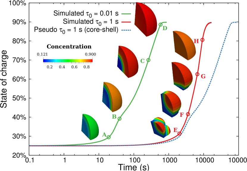
Figure 5: The SOC with corresponding concentration profile of the particle at different charging rate. A fast reaction (green line) can give a core-shell structure while a slow reaction (red line) will not preserve the core-shell. However, the latter can give a more robust reaction after the phase segregation occurs. The pseudo plot is the curve when the core-shell structure is enforced when $\displaystyle\tau_{0}=$\displaystyle 1\text{\,}\mathrm{s}$$.

The solid lines describe the simulated SOC with respect to time. Both curves show the same tendency of the reaction, which is fairly fast at the beginning and slows down towards the end of the charge. Both of them show an acceleration of reaction when the particle is charged at roughly $\displaystyle 30\text{\,}\mathrm{\char 37\relax}$ (A, E), because in both cases the phases start to form and the overpotential $\displaystyle\eta^{s}$ increases rapidly as the concentration increases, which can be seen in Figure 4 (a).

However, the phase segregation is very different in the two cases. The green line shows that, when the reaction is fast enough, a core-shell structure can be achieved. This is in agreement with the predictions in the work of Singh et al. [31], which stated that in an isotropic bulk-transport-limited case, where the bulk diffusion is much slower than the reaction, the phase boundary is driven largely by the incoming flux, thus a shrinking-core profile being formed. On the other hand, as shown by the red line, when the surface reaction is slow enough, the species can be always equilibrated by the bulk transport. In this case, the spinodal decomposition, or nucleation, initiates from the surface, where the dynamics of reaction can greatly fluctuate the species concentration. They are very unstable inside the spinodal region. The reaction in the core-shell structure slows down as the two phase region is finally formed (B, C), because the outer shell approaches a full lithiation. However, in the other case, the reaction maintains its rate (F, G) until the phase segregation is suppressed. Based on the simulation results of the case $\displaystyle\tau_{0}=$\displaystyle 0.01\text{\,}\mathrm{s}$$, one can predict the state of charge curve for $\displaystyle\tau_{0}=1s$ when the core-shell structure in enforced, simply by scaling the time of the fast case by a factor of 100. For comparison, this predicted result is shown by the curve in blue color in Fig. 5. It shows that if the core-shell structure is maintained, the lithiation process becomes slower than that in the case when the particle is free to adjust the phase pattern for a more robust reaction.

5.2 Reaction inside the interface

To investigate the reaction in different phases and the phase interface, a square plate with isotropic and anisotropic chemical properties is studied in this section. The geometry is given in Figure 7. No preferred direction for the reaction is assumed. Therefore, in the simulation, the reaction will take place in all six surfaces of the plate and the reaction rate is governed by the chemical state at each position on the surface. The anisotropic interfacial parameter $\displaystyle\kappa$ and diffusivity D in different directions is given in Tabel 7. In this model, the mechanical part is disregarded.

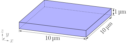
Figure 6: Sketch and measurements of the square plate problem. All six surfaces of the plate are exposed to the electrolyte, therefore electrochemical reaction can take place on all sides.

Interfacial Parameter	$\displaystyle\kappa_{x}$	$\displaystyle 1.0\text{\times}{10}^{-10}\text{\,}\mathrm{J}\text{\,}{\mathrm{mol}}^{-1}\text{\,}{\mathrm{m}}^{-2}$
	$\displaystyle\kappa_{y}$	$\displaystyle 1000\,\kappa_{x}$
	$\displaystyle\kappa_{z}$	$\displaystyle 1000\,\kappa_{x}$
	Dx	$\displaystyle 7.08\text{\times}{10}^{-15}\text{\,}{\mathrm{m}}^{2}\text{\,}{\mathrm{s}}^{-1}$
Diffusivity	Dy	1000 Dx
	Dz	1000 Dx
Sing. reac.	$\displaystyle\tau_{0}$	$\displaystyle 1\text{\,}\mathrm{s}$

Figure 7: Anisotropic interface and diffusivity parameters for the plate problem. For the isotropic case, the parameters for x direction are used for all three directions. All other parameters are given in Table 1.

In the isotropic case, as shown in Figure 8, the flux is marching towards the interior from all four sides, and the phase segregation of a Li-rich frame and a Li-deficient depression forms. As more flux comes in, there arises an island of Li-rich phase in the middle of the Li-poor phase. This can be explained by the dynamics of diffusion and reaction, where the whole system is perturbed strongly and it is easy to achieve a phase segregation once the magnitude of fluctuation is large enough. As for the reaction, by comparing the concentration profile and the reaction rate, one can observe that the reaction peaks at the interface front, where the concentration gradient is very high. In the two homogeneous phases, the reaction is relatively slow, especially in the Li-rich phase, where the reaction almost stops. This low efficiency of reaction in the Li-rich phase explains again why the core-shell structure is lithiated much slower than the other, studied in the last subsection.

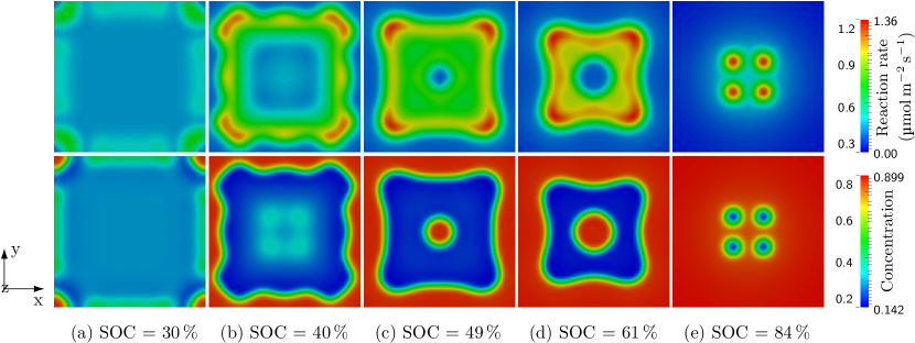
Figure 8: Contour plot of the reaction rate and the concentration SOC in an isotropic diffusion process. The peak of the reaction will always take place near the interface.

Figure 9 shows the case of an anisotropic diffusion. As explained in the section 2.2, the interfacial parameter is chosen in such a way that $\displaystyle\kappa_{x}:\kappa_{y}:\kappa_{z}=\mathrm{D}_{x}:\mathrm{D}_{y}:\mathrm{D}_{z}$. In the simulation, the diffusion in x direction is set to be slowest. Note that even though diffusivity in y, z direction is the same, in z-direction lithium sites are filled faster than in y-direction. This is due to the fact that the dimension in z-direction is smaller than that in y-direction. In contrast to the isotropic case, phase segregation initiates from the two ends although the reaction takes place in all six sides of x axis. As time goes on, the phase interface marches towards the center. A third Li-rich phase appears in the middle when SOC is approximately $\displaystyle 50\text{\,}\mathrm{\char 37\relax}$, thus the formation of stripes appears. This result supports the domino-cascade model of LiFePO₄, which was proposed in the work of Delma et al. [32]

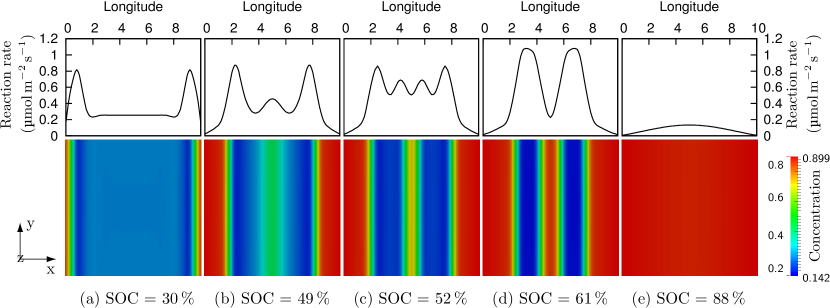
Figure 9: Contour plot of the concentration and plot of the reaction rate along the direction of the slowest diffusion (x direction) at different SOC in an anisotropic diffusion process.

These two cases are extreme. However, with proper implementation of crystal anisotropy, by filling the diffusion matrix also in the off-diagonal entries, one can also achieve a core-shell structure with a polygon core, as observed in the work of Liu et al. [33].

5.3 Reaction on the crack surface

As final example, we simulate an infinitely long cylinder with two initial parallel longitudinal cracks on its exterior. The problem is illustrated in Figure 11, and the corresponding parameters are given in Table 11. The electrode/electrolyte voltage drop is given such that Li is extracted from the cylinder. The reaction only takes place on the cylindrical surface and the crack surface. As it is explained in section 3.2, the reaction on the crack surface is approximated by the weighted source in the phase-field theory. In order to reach the diffusive profile for the initial crack, the reaction is set to be zero for the first 3 seconds.

Figure 10: Illustration and measurements of an infinite cylinder with initial cracks. One quarter of a disc with a thickness of $\displaystyle 1\text{\,}\mathrm{\SIUnitSymbolMicro m}$ under plane strain assumption is simulated.

Voltage drop eld./ely. ($\displaystyle\mathbb{\Delta}\phi$)	$\displaystyle 4.88\text{\,}\mathrm{mV}$
Single reac. step time ($\displaystyle\tau_{0}$)	$\displaystyle 0.01\text{\,}\mathrm{s}$
Initial concentration ($\displaystyle c_{0}$)	$\displaystyle 0.8\text{\,}$
Energy release rate ($\displaystyle\mathcal{G}_{c}$)	$\displaystyle 6\text{\times}{10}^{-2}\text{\,}\mathrm{N}\text{\,}{\mathrm{m}}^{-1}$
Crack lenth scale ($\displaystyle\epsilon$)	$\displaystyle 0.05\text{\,}\mathrm{\SIUnitSymbolMicro m}$
Crack mobility (Mc)	$\displaystyle 1.3\text{\times}{10}^{-3}\text{\,}\mathrm{J}\text{\,}{\mathrm{m}}^{-3}\text{\,}{\mathrm{s}}^{-1}$

Figure 11: Simulation parameters for the crack propagation problem. Others parameters can be found in Table 1.

The results of the crack propagation is shown in Figure 12. Initially, the concentration field is homogeneous. As the outer layer loses more lithium, a two-phase profile appears. It should be noted that at the crack tip lithium can be supplied quickly from the unbroken material. In fact, due to the large tensile stresses at the crack tip, the drift effect of the mechanical field towards the crack tip becomes prominent. This effect can be seen more clearly in Figure 12(c), where the phase interface on the crack surface is far behind that in the other part of the material.

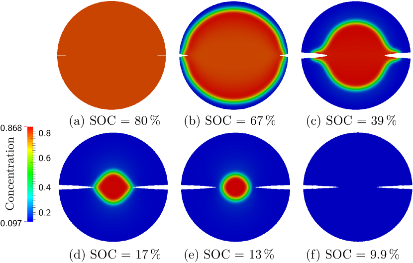
Figure 12: Crack propagation under delithiation and phase segregation. a) Initial homogeneous state. b) Formation of phase segregation initiates the crack propagation. c) Intermediate stage when the crack propagates faster than phase interface. d) Stage when phase interface leaves the crack tip. e) Stage when phase interface moves towards center. d) Final stage when the reaction stops.

On the other hand, due to the loss of lithium, the outer layer turns to shrink. Because of this mismatch with the interior Li-rich phase, tensile circumferential stresses arise in the outer layer, which drives the crack to propagate. At the first stage, the crack propagates faster than the interface. It then slows down, until the phase interface runs over the crack tip. After the phase interface leaves the crack, the propagation of crack turns to stop, due to the decrease of the driving force. However, the phase interface continues to move. The Li-rich phase gradually reforms into a circular. At the end of the simulation, the whole material is almost fully delithiated, and the reaction stops. It should be mentioned that the interplay between the phase segregation and the crack propagation can strongly depend on the choice of the kinetics parameters. A more comprehensive study on this topic will be carried out in the future.

During the whole process, lithium can indeed be released on the crack surface. To check the approximated reaction on the crack surface, the reaction and the corresponding concentration profile on the circular plate at SOC = $\displaystyle 40\text{\,}\mathrm{\char 37\relax}$ are demonstrated in Fig. 13. At this state, on the crack surface both phases and phase interface are exposed to the electrolyte. By comparing these two plots, it can be seen that near the crack surface, the reaction peaks in the neighborhood of the interface and gradually diffuses into the bulk. In the Li-poor region, the reaction almost vanishes, while towards the crack tip the reaction is rather strong.

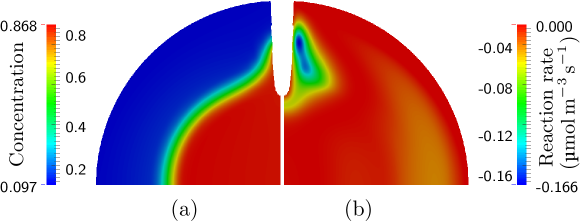
Figure 13: Reaction rate at the crack interface. a) The concentration profile when SOC = $\displaystyle 40\text{\,}\mathrm{\char 37\relax}$. b) The simulated reaction rate around the crack interface.

6 Conclusion

In this paper, the electrochemical reaction in the lithium ion batteries is studied by using phase-field modeling of fracture coupled with anisotropic Cahn-Hilliard-type diffusion in the large deformation regime.

The reaction on the surface is modeled through a modified Butler-Volmer equation, taking into account the influence of phase separation on the surface. The reaction on the crack surface is considered as a source term within the volume weighted by a damage-variable-related term to constrain the reaction to take place only on the transition zone between the unbroken and broken state.

Three examples are carried out to study different aspects. The first example of an isotropic sphere shows that the ratio of the timescale of the reaction and diffusion greatly influences the phase segregation of the material: a fast reaction gives a “shrinking core” while a slow reaction has the nucleation initiated already from the surface. In turn, the phase segregation also influences the real reaction rate through the electrochemical potential on the surface. When a core-shell structure is formed, the highly homogeneous concentration on the surface prevents the lithium from further inserting into the particle. However, an uneven distribution of the concentration, although accompanied by a highly distorted surface, can give a much more robust reaction in the long run. In the second example, the reaction on the interface of two phases in an isotropic diffusion and anisotropic diffusion is studied. Results show that, both in isotropic and anisotropic cases, the reaction rate peaks near the interface, where there exists a large concentration gradient. The last example shows the reaction on the crack surface. It is shown that the crack evolution can be driven by a outflow of the species when the material exhibits a phase segregation behavior. The electrochemical reaction on the newly created crack surfaces has been discussed, along with the interaction between the crack propagation and the phase segregation process.

References

- [1] G. K. Singh, G. Ceder, M. Z. Bazant, Intercalation dynamics in rechargeable battery materials: General theory and phase-transformation waves in LiFePO4, Electrochimica Acta 53 (26) (2008) 7599–7613. doi:10.1016/j.electacta.2008.03.083.
- [2] P. Bai, D. A. Cogswell, M. Z. Bazant, Suppression of Phase Separation in LiFePO4 Nanoparticles During Battery Discharge, Nano Letters 11 (11) (2011) 4890–4896. doi:10.1021/nl202764f.
- [3] S. Dargaville, T. W. Farrell, The persistence of phase-separation in LiFePO4 with two-dimensional Li+ transport: The Cahn-Hilliard-reaction equation and the role of defects, Electrochimica Acta 94 (2013) 143–158. doi:10.1016/j.electacta.2013.01.082.
- [4] C. V. Di Leo, E. Rejovitzky, L. Anand, A Cahn-Hilliard-type phase-field theory for species diffusion coupled with large elastic deformations: Application to phase-separating Li-ion electrode materials, Journal of the Mechanics and Physics of Solids 70 (2014) 1–29. doi:10.1016/j.jmps.2014.05.001.
- [5] H. Dal, C. Miehe, Computational electro-chemo-mechanics of lithium-ion battery electrodes at finite strains, Computational Mechanics 55 (2) (2014) 303–325. doi:10.1007/s00466-014-1102-5.
- [6] J. Christensen, J. Newman, Stress generation and fracture in lithium insertion materials, Journal of Solid State Electrochemistry 10 (5) (2006) 293–319. doi:10.1007/s10008-006-0095-1.
- [7] X. Zhang, W. Shyy, A. M. Sastry, Numerical simulation of intercalation-induced stress in Li-ion battery electrode particles, Journal of The Electrochemical Society 154 (10) (2007) A910–A916. doi:10.1149/1.2759840.
- [8] P. Stein, B. Xu, 3D Isogeometric Analysis of intercalation-induced stresses in Li-ion battery electrode particles, Computer Methods in Applied Mechanics and Engineering 268 (2014) 225–244. doi:10.1016/j.cma.2013.09.011.
- [9] S. Huang, F. Fan, J. Li, S. Zhang, T. Zhu, Stress generation during lithiation of high-capacity electrode particles in lithium ion batteries, Acta Materialia 61 (12) (2013) 4354–4364. doi:10.1016/j.actamat.2013.04.007.
- [10] M. Huttin, M. Kamlah, Phase-field modeling of stress generation in electrode particles of lithium ion batteries, Applied Physics Letters 101 (13) (2012) 133902. doi:10.1063/1.4754705.
- [11] A.-C. Walk, M. Huttin, M. Kamlah, Comparison of a phase-field model for intercalation induced stresses in electrode particles of lithium ion batteries for small and finite deformation theory, European Journal of Mechanics - A/Solids 48 (2014) 74–82. doi:10.1016/j.euromechsol.2014.02.020.
- [12] J. Rohrer, K. Albe, Insights into Degradation of Si Anodes from First-Principle Calculations, The Journal of Physical Chemistry C 117 (37) (2013) 18796–18803. doi:10.1021/jp401379d.
- [13] J. Rohrer, A. Moradabadi, K. Albe, P. Kaghazchi, On the origin of anisotropic lithiation of silicon, Journal of Power Sources 293 (2015) 221–227. doi:10.1016/j.jpowsour.2015.05.057.
- [14] G. Chen, X. Song, T. J. Richardson, Electron Microscopy Study of the LiFePO4 to FePO4 Phase Transition, Electrochemical and Solid-State Letters 9 (6) (2006) A295–A298. doi:10.1149/1.2192695.
- [15] C. V. Ramana, A. Mauger, F. Gendron, C. M. Julien, K. Zaghib, Study of the Li-insertion/extraction process in LiFePO4/FePO4, Journal of Power Sources 187 (2) (2009) 555–564. doi:10.1016/j.jpowsour.2008.11.042.
- [16] D. Schneider, M. Selzer, J. Bette, I. Rementeria, A. Vondrous, M. J. Hoffmann, B. Nestler, Phase-Field Modeling of Diffusion Coupled Crack Propagation Processes, Advanced Engineering Materials 16 (2) (2014) 142–146. doi:10.1002/adem.201300073.
- [17] L. Liang, M. Stan, M. Anitescu, Phase-field modeling of diffusion-induced crack propagations in electrochemical systems, Applied Physics Letters 105 (16) (2014) 163903. doi:10.1063/1.4900426.
- [18] P. Zuo, Y.-P. Zhao, A phase field model coupling lithium diffusion and stress evolution with crack propagation and application in lithium ion batteries, Physical Chemistry Chemical Physics 17 (1) (2014) 287–297. doi:10.1039/C4CP00563E.
- [19] C. Miehe, H. Dal, A. Raina, A phase field model for chemo-mechanical induced fracture in lithium-ion battery electrode particles, International Journal for Numerical Methods in Engineering (2015) n/a–n/adoi:10.1002/nme.5133.
- [20] M. Z. Bazant, Theory of Chemical Kinetics and Charge Transfer based on Nonequilibrium Thermodynamics, Accounts of Chemical Research 46 (5) (2013) 1144–1160. doi:10.1021/ar300145c.
- [21] J. W. Cahn, J. E. Hilliard, Free energy of a nonuniform system. I. interfacial free energy, The Journal of Chemical Physics 28 (26) (1958) 258–267. doi:10.1016/j.electacta.2008.03.083.
- [22] B. Bourdin, G. A. Francfort, J.-J. Marigo, The Variational Approach to Fracture, Journal of Elasticity 91 (1-3) (2008) 5–148. doi:10.1007/s10659-007-9107-3.
- [23] Y. Zhao, P. Stein, B.-X. Xu, Isogeometric analysis of mechanically coupled Cahn–Hilliard phase segregation in hyperelastic electrodes of Li-ion batteries, Computer Methods in Applied Mechanics and Engineering 297 (2015) 325–347. doi:10.1016/j.cma.2015.09.008.
- [24] C. Kuhn, R. Müller, A continuum phase field model for fracture, Engineering Fracture Mechanics 77 (18) (2010) 3625–3634. doi:10.1016/j.engfracmech.2010.08.009.
- [25] C. Kuhn, A. Schlüter, R. Müller, On degradation functions in phase field fracture models, Computational Materials Science 108, Part B (2015) 374–384. doi:10.1016/j.commatsci.2015.05.034.
- [26] A. Schlüter, A. Willenbüücher, C. Kuhn, R. Müller, Phase field approximation of dynamic brittle fracture, Computational Mechanics 54 (5) (2014) 1141–1161. doi:10.1007/s00466-014-1045-x.
- [27] C. Miehe, M. Hofacker, F. Welschinger, A phase field model for rate-independent crack propagation: Robust algorithmic implementation based on operator splits, Computer Methods in Applied Mechanics and Engineering 199 (45-48) (2010) 2765 – 2778. doi:http://dx.doi.org/10.1016/j.cma.2010.04.011.
- [28] C. Miehe, L.-M. Sch Phase field modeling of fracture in multi-physics problems. Part I. Balance of crack surface and failure criteria for brittle crack propagation in thermo-elastic solids, Computer Methods in Applied Mechanics and Engineering 294 (2015) 449 – 485. doi:http://dx.doi.org/10.1016/j.cma.2014.11.016.
- [29] M. J. Borden, C. V. Verhoosel, M. A. Scott, T. J. R. Hughes, C. M. Landis, A phase-field description of dynamic brittle fracture, Computer Methods in Applied Mechanics and Engineering 217–220 (2012) 77–95. doi:10.1016/j.cma.2012.01.008.
-
[30]
R. L. Taylor, FEAP - finite
element analysis program (2014).
URL http://www.ce.berkeley.edu/projects/feap - [31] G. K. Singh, G. Ceder, M. Z. Bazant, Intercalation dynamics in rechargeable battery materials: General theory and phase-transformation waves in LiFePO4, Electrochimica Acta 53 (26) (2008) 7599–7613. doi:10.1016/j.electacta.2008.03.083.
- [32] C. Delmas, M. Maccario, L. Croguennec, F. Le Cras, F. Weill, Lithium deintercalation in LiFePO4 nanoparticles via a domino-cascade model, Nature Materials 7 (8) (2008) 665–671. doi:10.1038/nmat2230.
- [33] X. H. Liu, L. Zhong, S. Huang, S. X. Mao, T. Zhu, J. Y. Huang, Size-Dependent Fracture of Silicon Nanoparticles During Lithiation, ACS Nano 6 (2) (2012) 1522–1531. doi:10.1021/nn204476h.