Deforming convex projective manifolds

Abstract.

We study a properly convex real projective manifold with (possibly empty) compact, strictly-convex boundary, and which consists of a compact part plus finitely many convex ends. We extend a theorem of Koszul which asserts that for a compact manifold without boundary the holonomies of properly convex structures form an open subset of the representation variety. We also give a relative version for non-compact $(G,X)$-manifolds of the openness of their holonomies.

Given a subset $\Omega\subset{\mathbb{R}}P^{n}$ the frontier is ${\operatorname{Fr}}(\Omega)={\rm cl}({\Omega})\setminus\operatorname{int}(\Omega)$ and the boundary is $\partial\Omega=\Omega\cap{\operatorname{Fr}}(\Omega)$. A properly convex projective manifold is $M=\Omega/\Gamma,$ where $\Omega\subset{\mathbb{R}}P^{n}$ is a convex set with non-empty interior, and ${\rm cl}({\Omega})$ does not contain any ${\mathbb{RP}}^{1}$, and $\Gamma\subset\operatorname{PGL}(n+1,{\mathbb{R}})$ acts freely and properly discontinuously on $\Omega$. If, in addition, ${\operatorname{Fr}}(\Omega)$ contains no line segment then $M$ and $\Omega$ are strictly-convex. The boundary of $M$ is strictly-convex if $\partial\Omega$ contains no line segment.

If $M$ is a compact $(G,X)$-manifold then a sufficiently small deformation of the holonomy gives another $(G,X)$-structure on $M$. In [25, 26] Koszul proved a similar result holds for closed, properly convex, projective manifolds. In particular, nearby holonomies continue to be discrete and faithful representations of the fundamental group.

Koszul’s theorem cannot be generalized to the case of non-compact manifolds without some qualification—for example, a sequence of hyperbolic surfaces whose completions have cone singularities can converge to a hyperbolic surface with a cusp. The holonomy of a cone surface in general is neither discrete nor faithful. Therefore we must impose conditions on the holonomy of each end.

If $M$ is a geometrically finite hyperbolic manifold $M$ with a convex core that has compact boundary, then every end of $M$ is topologically a product, and is foliated by strictly-convex hypersurfaces. These hypersurfaces are either convex towards $M$ so that cutting along one gives a submanifold of $M$ with convex boundary, and the holonomy of the end contains only hyperbolics; or else convex away from $M$, in which case the end is a cusp and the holonomy of the end contains only parabolics.

This paper studies properly convex manifolds whose ends are either convex towards or away from $M$. An end that is convex towards $M$ may be compactified by adding a convex boundary. Generalized cusps are those that are convex away from $M$ with virtually nilpotent fundamental group. The holonomy of a generalized cusp may contain both hyperbolic and parabolic elements.

Definition 0.1.

A generalized cusp is a properly convex manifold $C$ homeomorphic to $\partial C\times[0,\infty)$ with compact, strictly-convex boundary and with $\pi_{1}C$ virtually nilpotent.

For instance, all ends of a finite volume hyperbolic manifold are generalized cusps. For an $n$–manifold $M$, possibly with boundary, define $\operatorname{Rep}(\pi_{1}M)=\operatorname{Hom}(\pi_{1}M,\operatorname{GL}(n+1,{\mathbb{R}}))$ and $\operatorname{Rep_{ce}}(M)$ to be the subset of $\operatorname{Rep}(\pi_{1}M)$ consisting of holonomies of properly convex structures on $M$ with $\partial M$ strictly-convex, and such that each end is a generalized cusp. A group $\Gamma\subset\operatorname{GL}(n+1,{\mathbb{R}})$ is a virtual flag group if it contains a subgroup of finite index that is conjugate into the upper-triangular group. The set of virtual flag groups is written $\operatorname{VFG}$.

Theorem 0.2.

Suppose $N$ is a compact connected $n$–manifold and $\mathcal{V}=\cup_{i}V_{i}\subseteq\partial N$ is the union of some of the boundary components of $N.$ Let $M=N\setminus\mathcal{V}$. Assume $\pi_{1}V_{i}$ is virtually nilpotent for each $i$. Let $B_{i}\cong V_{i}\times[0,1)$ be the end of $M$ corresponding to $V_{i}$. Then $\operatorname{Rep_{ce}}(M)$ is an open subset of

$$\operatorname{VFG}(M):=\{\rho\in\operatorname{Rep}(\pi_{1}M):\forall i\ \rho(\pi_{1}B_{i})\in\operatorname{VFG}\}.$$

A similar statement holds for orbifolds since a properly convex orbifold has a finite cover which is a manifold, and the property of being properly convex is unchanged by coverings. This theorem is a consequence of our main theorem (6.29) that a certain map is open. By (6.11) $\rho(\pi_{1}B_{i})\in\operatorname{VFG}$ iff there is a finite index subgroup $\Gamma<\rho(\pi_{1}B_{i})$ such that every eigenvalue of every element of $\Gamma$ is real.

There is a Margulis lemma for properly convex manifolds that says the local fundamental group is virtually nilpotent (0.1) in Cooper, Long and Tillmann [13], also Crampon and Marquis [14]. There is a thick-thin decomposition for strictly convex manifolds (0.2) in [13], also Crampon and Marquis [15]; but not for properly convex manifolds. Each component of the thin part of a strictly convex manifold is a Margulis tube or a cusp and has virtually nilpotent fundamental group consisting of parabolics. This motivates the definition of generalized cusp above. There is a discussion of cusps in properly convex manifolds in §5 of [13].

Here is some intuition for the proof of (0.2). Many of the ideas are already present for surfaces. Suppose $M$ is a projective compact surface without boundary. There is a developing map $\operatorname{dev}:\widetilde{M}\rightarrow{\mathbb{RP}}^{2}$. If $M$ is properly convex then this map is injective and the image is a domain $\Omega\subset{\mathbb{R}}^{2}$ bounded by a convex closed curve $C\subset{\mathbb{R}}^{2}$. There is a compact polygonal fundamental domain $D\subset\Omega$ and the images of $D$ under the holonomy $\rho:\pi_{1}M\rightarrow\Gamma\subset\operatorname{PGL}(3,{\mathbb{R}})$ tesselate $\Omega$. Small images of $D$ accumulate on $C$. Suppose $\rho^{\prime}$ is a nearby homomorphism. Our aim is to show there is a convex closed curve $C^{\prime}$ close to $C$ that bounds a domain $\Omega^{\prime}$ that is preserved by $\Gamma^{\prime}=\rho^{\prime}(\pi_{1}M)$.

The convexity of $C$ is a phenomenon that takes place at infinity with regard to $\Omega$. A priori, there is no reason to expect this phenomenon to be stable with respect to small deformations. A finite generating set for $\pi_{1}M$ determines a word metric on $\pi_{1}M$. If $g\in\pi_{1}M$ is not too far from the identity in the word metric then $\rho^{\prime}(g)$ and $\rho(g)$ are close and send $D$ to almost the same set. However, for large elements $g$, one loses control, and there is no obvious reason why images of $D$ should accumulate on some convex curve $C^{\prime}$. Thus convexity of $C=\partial\Omega$ is a limiting feature of large group elements in $\pi_{1}M$, and this might be destroyed by arbitrarily small deformations $\rho^{\prime}$. In fact this is what happens with the example of surfaces with cone singularities discussed above. Convexity is stable for closed surfaces for reasons that we now outline.

Let $U\subset{\mathbb{R}}^{3}$ be the half space $x_{3}\geq 0$ and $P=\partial U$ the plane $x_{3}=0.$ Suppose $D\subset U$ is a disc, bounded by the simple closed curve $C=D\cap P$, and $S=\operatorname{int}(D)$. If $S$ is convex down then $C$ is convex, and bounds a convex domain $\Omega\subset P$, and $S$ is a graph over $\Omega$. The condition that $S$ is convex down is a condition over (finite) points in $\Omega$ rather than a condition at infinity. One might imagine that $S$ is the surface of a mountain. If this surface is convex then the boundary of the base of the mountain is also convex.

The tautological line bundle $\xi M$ over $M$ is an affine manifold. For a properly convex projective structure on $M$, there is a section $\sigma(M)$ of this bundle that is a surface in $\xi M$ which is strictly convex in the sense that the Hessian is strictly positive. The image of the universal cover of $\sigma(M)$ under the developing map is a surface $S\subset{\mathbb{R}}^{3}$ that limits on the sphere at infinity. By viewing ${\mathbb{R}}^{3}\subset{\mathbb{RP}}^{3}$, and choosing a suitable new affine patch where the sphere at infinity becomes $P$, we can instead view $S$ as a surface in $U$ as above, and then $M=\Omega/\rho(\pi_{1}M)$. If $M$ is compact then $\sigma(M)$ is compact. A small deformation, $M^{\prime}$ of $M$, gives a nearby strictly-convex surface $\sigma(M^{\prime})$ in $\xi M^{\prime}$, that develops to another convex surface $S^{\prime}$ in ${\mathbb{R}}^{3}$ and gives a convex domain $\Omega^{\prime}\subset P$. This is the intuition for Koszul’s theorem when $M$ is closed.

Now suppose that $M$ is a compact manifold, $N$, union a (generalized) cusp $C$. One first shows that for the deformed cusp $C^{\prime}$ that $\xi C^{\prime}$ contains a nearby strictly convex surface ${\sigma(C^{\prime}})$. Since $N$ is compact $\xi N^{\prime}$ contains a nearby convex surface $\sigma(N^{\prime})$. One now deforms and joins $\sigma(N^{\prime})$ and $\sigma(C^{\prime})$, maintaining convexity, to obtain a strictly-convex hypersurface in $\xi M^{\prime}$. This implies $M^{\prime}$ is properly convex.

Section 1 describes the $(G,X)$-Extension Theorem (1.7). This generalizes a well-known result for compact manifolds (the holonomies of $(G,X)$-structures form an open subset of the representation variety) by providing a relative version. Section 2 recalls the definition and properties of the tautological bundle. Section 3 reviews Hessian metrics and gives a characterization of properly convex manifolds in terms of the existence of a certain kind of Hessian metric on the tautological line bundle. Section 4 shows that various functions on properly convex projective manifolds are uniformly bounded, including a proof of the folklore result that they admit Riemannian metrics with all sectional curvatures bounded in terms of dimension.

The Convex Extension Theorem (5.8) is a version of (1.7) for properly convex manifolds with strictly-convex boundary. A consequence is (0.3) below. Roughly this says that if you can convexly deform the ends of a properly convex manifold then you can convexly deform the manifold. There is no assumption that the fundamental group of an end is virtually nilpotent for this result.

Theorem 0.3.

Suppose $M=A\cup\mathcal{B}$ is a properly convex manifold with (possibly empty) compact strictly-convex boundary, and $A$ is a compact connected submanifold of $M$ with $\partial A=\partial M\sqcup\partial\mathcal{B}$, and $\mathcal{B}\cong\partial\mathcal{B}\times[0,\infty)=B_{1}\sqcup\cdots\sqcup B_{k}$, and each $B_{i}$ is connected and $\pi_{1}$-injective in $M$.

Suppose $\rho:(-1,1)\to\operatorname{Rep}(\pi_{1}M)$ is continuous and $\rho_{t}:=\rho(t)$ and $\rho_{0}$ is the holonomy of $M$. Let ${\mathfrak{C}}$ denote the space of closed subsets of ${\mathbb{RP}}^{n}$ with the Hausdorff topology. Suppose for all $1\leq i\leq k$ and all $t\in(-1,1)$ that

• there is a properly convex set $\Omega_{i}(t)\subset{\mathbb{RP}}^{n},$ that is preserved by $\rho_{t}(\pi_{1}B_{i}),$

• $P_{i}(t)=\Omega_{i}(t)/\rho_{t}(\pi_{1}B_{i})$ is a properly convex manifold and $\partial P_{i}(t)$ is strictly-convex,

• there is a projective diffeomorphism from $P_{i}(0)$ to $B_{i},$

• $P_{i}(t)$ is diffeomorphic to $B_{i},$

• the two maps $t\mapsto{\rm cl}(\Omega_{i}(t))$ and $t\mapsto{\rm cl}(\partial\Omega_{i}(t))$ into ${\mathfrak{C}}$ are continuous.

Then there is $\epsilon>0$ such that for all $t\in(-\epsilon,\epsilon)$ there is a properly convex projective structure on $M$ with holonomy $\rho(t)$ such that $\partial M$ is strictly-convex and $B_{i}$ is projectively diffeomorphic to $P_{i}(t)$.

If $\Omega\subset{\mathbb{RP}}^{n}$ we write $\operatorname{PGL}(\Omega)$ for the subgroup of $\operatorname{PGL}(n+1,{\mathbb{R}})$ that preserves $\Omega$. Section 6 proves that generalized cusps contain homogeneous cusps (6.3):

Theorem 0.4.

Suppose $C=\Omega/\Gamma$ is a generalized cusp. Then $C$ contains a generalized cusp $C^{\prime}=\Omega^{\prime}/\Gamma$ such that $\operatorname{PGL}(\Omega^{\prime})$ acts transitively on $\partial\Omega^{\prime}$.

An algebraic argument (6.18) uses $\Gamma$ is virtually nilpotent to show that if $C=\Omega/\Gamma$ is a generalized cusp then $\Gamma$ has a finite index subgroup that is a lattice in a connected Lie group $T=T(\Gamma)$ that is conjugate into the upper-triangular group.

Next (6.24) shows that the $T$-orbit of some point $p\in\Omega$ is a strictly-convex hypersurface $S=T\cdot p$. The convex hull of $S$ is a domain $\Omega_{T}$ that is preserved by all of $\Gamma$, and we may shrink $C$ to be $\Omega_{T}/\Gamma$ giving (0.4).

From (0.4) it follows that generalized cusps are stable (6.28): if $\Gamma$ is deformed to a nearby virtual flag group $\Gamma^{\prime}$, then $T^{\prime}=T(\Gamma^{\prime})$ is a nearby Lie group, so $S^{\prime}=T(\Gamma^{\prime})\cdot p$ is a nearby strictly-convex hypersurface which gives a nearby domain $\Omega_{T^{\prime}}$ and a nearby generalized cusp $C^{\prime}=\Omega_{T^{\prime}}/\Gamma^{\prime}$.

The convex extension theorem and the stability of generalized cusps imply the main theorem (0.2). Ballas, Cooper and Leitner [3] classify generalized cusps, and their properties are studied. This classification for 3-manifolds is given without proof in section 7.

A function is Hessian-convex if it is smooth and has positive definite Hessian. This property is preserved by composition with diffeomorphisms that are close to affine. Section 8 reviews various types of convexity and contains a theorem about approximating strictly-convex functions on affine manifolds by Hessian-convex ones. As a result, for our purposes strictly and Hessian convex are more or less equivalent. Section 9 is a short proof of Benzécri’s Theorem. We have put these results at the end of the paper with the intention of not breaking the narrative.

There is an entirely PL approach to (0.2) which, however, we do not develop in this paper. It is based on using the convex hull of the orbit of one point instead of a characteristic surface.

Theorem (0.2) does not always remain true if $\partial M$ is convex but not strictly-convex. However, in some cases, the theorem can still be applied. For instance, a hyperbolic manifold $M$ with compact, totally geodesic boundary is a submanifold of a finite volume hyperbolic manifold with strictly-convex smooth boundary obtained by fattening. In particular, any small deformation in $\operatorname{PGL}(4,\mathbb{R})$ of the holonomy in $PO(3,1)$ of a compact Fuchsian manifold is the holonomy of a strictly-convex projective structure on (surface)$\times[0,1].$

The reader only interested in the proof of (0.2) when $M$ is compact need only read section 1 up to (1.2), and then sections 2 to 4 stopping before (4.2). Those interested only in the proof of (0.3) can omit section 6.

Most of sections 1-4 is not new, and there is considerable overlap in the first 5 sections with the results and methods of Choi in [8]. Marquis determined the holonomies of properly convex surfaces with cusps [30] and [29]. In [12] Cooper and Long give a method of constructing fundamental domains for some strictly-convex manifolds with cusps. Using the main result of this paper, Ballas found new properly convex structures on the figure eight knot obtained by deforming the complete hyperbolic structure [2]. The type of geometry in a generalized cusp can change during a deformation. For example a generalized cusp with diagonal holonomy can transition to one with parabolic holonomy. This is related to the study of geometric transition, see Cooper, Danciger and Wienhard [11].

In section 5 of [13] there is a discussion of properly convex $n$-manifolds with parabolic holonomy. Such a manifold is diffeomorphic to a product $C\times{\mathbb{R}}$ and $\Gamma=\pi_{1}C$ is virtually nilpotent. The manifold $C$ is compact iff the Hirsch rank of $\Gamma$ is maximal: namely $(n-1)$. In [13] these cusps are called maximal, and it is shown in this case that $\Gamma$ is conjugate into $PO(n,1)$. In general, parabolics are not conjugate into $PO(n,1)$. In this paper frequent use is made of the fact that $\partial C$ is compact is equivalent to $H_{n-1}(C;\mathbb{Z}_{2})\cong\mathbb{Z}_{2}$. For consistency with [13] one might call such generalized cusps maximal. However, to keep this paper from becoming even longer, these are the only type of generalized cusp we consider, therefore we do not use the term maximal.

0.1. Acknowledgments

Work partially supported by U.S. National Science Foundation grants DMS 1107452, 1107263, 1107367 RNMS: GEometric structures And Representation varieties (the GEAR Network). Cooper was partially supported by NSF grants DMS 1065939, 1207068 and 1045292 and thanks IAS and the Ellentuck Fund for partial support. Long was partially supported by grants from the NSF. Tillmann was partially supported by Australian Research Council grant DP140100158. We thank the referee for an excellent job.

1. (G,X) structures and Extending Deformations

The goal of this section is a relative version of the well-known fact (1.2) that for compact manifolds the set of holonomies of $(G,X)$-structures is an open subset of the representation variety. The Extension Theorem (1.7) implies that if $\mathcal{B}$ is a codimension-0 submanifold of a connected manifold $M$ with $M\setminus\mathcal{B}$ compact and connected, then given a $(G,X)$-structure on $M$ with holonomy $\rho$, together with a nearby representation $\sigma$, and given a nearby $(G,X)$-structure on each component of $\mathcal{B}$ with holonomy the restriction of $\sigma$, there is a nearby $(G,X)$-structure on $M$ with holonomy $\sigma$ that extends the structure on $\mathcal{B}$.

A geometry is a pair $(G,X)$ where $G$ is a Lie group which acts transitively and real-analytically on a manifold $X$. A $(G,X)$-structure on a manifold $M$ (possibly with boundary) is a maximal atlas of charts which takes values in $X$, so that transitions maps are locally the restriction of elements of $G$. A map between $(G,X)$ manifolds is a $(G,X)$ map if locally it is conjugate via $(G,X)$-charts to an element of $G$.

Let $\pi:\widetilde{M}\to M$ be (a fixed choice for) the universal cover of $M$. We regard $\pi_{1}M$ to be defined as the group of covering transformations of this covering. A local diffeomorphism $f:\widetilde{M}\to X$ determines a $(G,X)$-structure on $\widetilde{M}$. If all the covering transformations are $(G,X)$-maps then there is a unique $(G,X)$-structure on $M$ such that the covering space projection is a $(G,X)$-map. In this case $f$ is called a developing map for this structure and determines a homomorphism $\operatorname{hol}=\mathcal{H}ol(f):\pi_{1}M\to G$ called holonomy.

For smooth manifolds $M^{m}$ and $N^{n}$ the set of smooth maps $C^{\infty}_{w}(M,N)$ has the weak topology [22, Hirsch page 35]. The space of diffeomorphisms ${\operatorname{Diff}}(M)$ is a subspace of $C^{\infty}_{w}(M,M)$. If $N=\mathbb{R}$ then $C^{\infty}_{w}(M):=C^{\infty}_{w}(M,\mathbb{R})$.

The set of all developing maps is denoted $\mathcal{D}ev(M,(G,X))$ or just $\mathcal{D}ev(M)$. The $(G,X)$-structure on $M$ given by $\operatorname{dev}\in\mathcal{D}ev(M)$ is written $(M,\operatorname{dev})$. There is a natural map of $\mathcal{D}ev(M)$ into $C_{w}^{\infty}(\operatorname{int}\widetilde{M},X)$ given by restricting the developing map to $\operatorname{int}\widetilde{M}$. This map is injective because $\operatorname{int}\widetilde{M}$ is dense in $\widetilde{M}$.

Definition 1.1.

The geometric topology on $\mathcal{D}ev(M)$ is the subspace topology from $C_{w}^{\infty}(\operatorname{int}\widetilde{M},X)$.

Thus two developing maps for $M$ are close if they are close on a large compact set in $\widetilde{M}$ that is disjoint from $\partial\widetilde{M}$. The following is due to Thurston [38], see also Goldman [19] and Choi [7]. The topology on $\operatorname{Hom}(\pi_{1}M,G)$ is the compact-open topology.

Proposition 1.2 (holonomy is open).

Suppose $M$ is a compact connected smooth manifold possibly with boundary. Then $\mathcal{H}ol:\mathcal{D}ev(M,(G,X))\to\operatorname{Hom}(\pi_{1}M,G)$ is continuous and open.

Given $\operatorname{dev}_{M}\in\mathcal{D}ev(M)$ and $\operatorname{dev}_{N}\in\mathcal{D}ev(N)$ a smooth map $f:M\to N$ is close to a $(G,X)$ map if it is covered by $F:\widetilde{M}\to\widetilde{N}$ and there is $g\in G$ such that $g\circ\operatorname{dev}_{N}\circ F$ is close to $\operatorname{dev}_{M}$ in $C^{\infty}_{w}(\widetilde{M},X)$. This means there is a large compact set $K\subset\operatorname{int}\widetilde{M}$ and some $g\in G$ such that for each $x\in K$ there is an open neighborhood $U\subset\widetilde{M}$ with $V=\operatorname{dev}_{M}(U\cap K)$ and the map $g\circ\operatorname{dev}_{N}\circ F\circ(\operatorname{dev}_{M}|_{U\cap K})^{-1}$ is close to the inclusion map $V\hookrightarrow X$ in $C^{\infty}_{w}(V,X)$. This notion of close depends on $\operatorname{dev}_{M}$ but not on the choice of developing map $\operatorname{dev}_{N}$ for a given $(G,X)$-structure on $N$.

There is a nice description of what it means for two developing maps in $\mathcal{D}ev(M)$ to be close when one of them is injective. Suppose $\operatorname{dev}\in\mathcal{D}ev(M)$ is injective and $\Omega=\operatorname{dev}(\widetilde{M})$ and $\rho=\mathcal{H}ol(\operatorname{dev})$ and $\Gamma=\rho(\pi_{1}M)$. Then $N=\Omega/\Gamma$ is a $(G,X)$ manifold that is $(G,X)$-diffeomorphic to $M$. We choose the universal cover $\widetilde{N}=\Omega$ then $\pi_{1}N=\Gamma$ by our definition as the group of covering transformations. There is a homeomorphism between spaces of developing maps $\mathcal{D}ev(M)\to\mathcal{D}ev(N)$.

Definition 1.3.

Replacing $\mathcal{D}ev(M)$ by $\mathcal{D}ev(N)$ is called choosing $\operatorname{dev}$ as the basepoint for the space of developing maps.

The developing map $\operatorname{dev}_{*}\in\mathcal{D}ev(N)$ for $N$ is the inclusion map $i:\widetilde{N}\hookrightarrow X$ and $\mathcal{H}ol(\operatorname{dev}_{*}):\Gamma\hookrightarrow G$ is also the inclusion map. If $N$ has no boundary then $\mathcal{D}ev(N)$ is a subspace of $C^{\infty}_{w}(\widetilde{N},X)$ so $\operatorname{dev}^{\prime}\in\mathcal{D}ev(N)$ is close to $\operatorname{dev}_{*}$ if $\operatorname{dev}^{\prime}$ is close to $i$ in $C^{\infty}_{w}(\widetilde{N},X)$.

The idea for the extension theorem is the following. Suppose $(M=A_{1}\cup A_{2},\operatorname{dev})$ is a $(G,X)$-manifold with holonomy $\rho$, and $C=A_{1}\cap A_{2}\cong\partial A_{i}\times[0,1]$ is a connected collar neighborhood of $\partial A_{i}$ and the inclusion map $C\hookrightarrow M$ is $\pi_{1}$-injective. Suppose $\rho^{\prime}:\pi_{1}M\rightarrow G$ is a nearby homomorphism and $(A_{i},\operatorname{dev}_{i}^{\prime})$ is a nearby $(G,X)$-structure to $(A_{i},\operatorname{dev}|A_{i})$ with holonomy $\rho^{\prime}|\pi_{1}A_{i}$. If $C$ is compact we show there is a nearby $(G,X)$-structure on $M$ obtained by gluing $(A_{1},\operatorname{dev}_{1}^{\prime})$ to $(A_{2},\operatorname{dev}_{2}^{\prime})$ by a $(G,X)$-diffeomorphism. This is done in (1.4) which uses analytic continuation to map the submanifold $C\subset(A_{1},\operatorname{dev}_{1}^{\prime})$ into $(A_{2},\operatorname{dev}_{2}^{\prime})$ by a $(G,X)$-diffeomorphism.

Lemma 1.4 (lifting developing maps).

In this statement all manifolds and maps are $(G,X)$. Suppose $N$ and $P$ are connected manifolds and $\theta:\pi_{1}N\to\pi_{1}P$ is a homomorphism such that $\operatorname{hol}_{N}=\operatorname{hol}_{P}\circ\theta$. Suppose $\pi_{P}:\widetilde{P}\to P$ and $\pi_{N}:\widetilde{N}\to N$ are universal covers and $i:Q\hookrightarrow\widetilde{N}$ is the inclusion map of a path-connected set $Q$ with $\pi_{N}(Q)=N$. Suppose $\operatorname{dev}_{N}\circ i:Q\to X$ lifts to a map $j:Q\to\widetilde{P}$ such that $\operatorname{dev}_{P}\circ j=\operatorname{dev}_{N}\circ i$. Then there is $k:N\to P$ covered by $\widetilde{k}:\widetilde{N}\to\widetilde{P}$ that extends $j$.

Proof.

Because the covering translates of $Q$ cover $\widetilde{N}$ and the manifolds $N$ and $P$ have (via $\theta$) the same holonomy, $j$ can be extended by analytic continuation to an equivariant $(G,X)$-map $\widetilde{k}:\widetilde{N}\to\widetilde{P}$. Equivariance implies $\widetilde{k}$ covers a $(G,X)$-map $k:N\to P$. ∎

For a closed manifold $M$ two nearby developing maps with the same holonomy differ by composition with a diffeomorphism of $M$ close to the identity. If $M$ has boundary then the boundary can move, so this result only holds outside a small neighborhood of the boundary, cf. the discussion in I.1.5 and I.1.6 leading to the proof of I.1.7.1 in Canary, Epstein and Green [6].

If $P$ is a smooth manifold then ${\operatorname{Diff}}_{0}(\widetilde{P},{P})\subset{\operatorname{Diff}}(\widetilde{P})$ is defined to be the identity component of the subgroup of diffeomorphisms that cover an element of ${\operatorname{Diff}}(P)$. The next result says that if two developing maps are close, and have the same holonomy then, after changing one by a small isotopy, the developing maps are equal on a compact submanifold in the interior.

Corollary 1.5.

Suppose $P$ is a smooth manifold. Let $\rho\in\operatorname{Hom}(\pi_{1}P,G)$ be the holonomy of $\operatorname{dev}\in\mathcal{D}ev(P,(G,X))$ and $\mathcal{D}ev_{\rho}(P)\subset\mathcal{D}ev(P)$ be the subspace of developing maps with holonomy $\rho$. Then the map ${\operatorname{Diff}}_{0}(\widetilde{P},{P})\to\mathcal{D}ev_{\rho}(P)$ given by $f\mapsto\operatorname{dev}\circ f$ is an open map.

It follows that, if $N$ is a compact codimension-0 manifold in the interior of $P$, and $\operatorname{dev}^{\prime}\in\mathcal{D}ev_{\rho}(P)$ is close enough to $\operatorname{dev}$, then there is $k\in{\operatorname{Diff}}(P)$ covered by $\widetilde{k}\in{\operatorname{Diff}}_{0}(\widetilde{P},{P})$ such that $\operatorname{dev}=\operatorname{dev}^{\prime}\circ\widetilde{k}$ on $N$, and $k$ is isotopic to the identity by a small isotopy supported in a small neighborhood of $N$.

Proof.

Let $\pi_{P}:\widetilde{P}\to P$ and $\pi_{N}:\widetilde{N}\to N$ be universal covers. Let $Q\subset\widetilde{N}$ be a compact connected manifold such that $\pi_{N}(Q)=N$. Since $\operatorname{dev}|_{Q}:Q\to X$ factors through the inclusion $j:Q\hookrightarrow\widetilde{P}$ and $(\pi_{p}\circ j)(Q)\subset\operatorname{int}(P)$ it follows that if $\operatorname{dev}^{\prime}$ is close enough to $\operatorname{dev}$ then $\operatorname{dev}^{\prime}|Q:Q\to X$ has a nearby lift $j^{\prime}:Q\to\widetilde{P}$. By (1.4) there is a $(G,X)$-map $k:(N,\operatorname{dev}^{\prime}|N)\to(P,\operatorname{dev}|N)$ that lifts to a map that extends $j^{\prime}$. If $\operatorname{dev}^{\prime}$ is sufficiently close to $\operatorname{dev}$, then $k$ is close to the inclusion, and the result now follows from the fact that a diffeomorphism (namely $k$) close to an inclusion is ambient isotopic to the inclusion by a small ambient isotopy, Lima [28]. ∎

Given a connected $\pi_{1}$-injective submanifold $B\subset M$ we fix a choice of some component $\widetilde{B}\subset\widetilde{M}$ of the preimage $B$ in the universal cover of $M$ and identify $\pi_{1}B$ with those covering transformations of $\widetilde{M}$ that preserve $\widetilde{B}$. If $\operatorname{dev}_{M}$ is a developing map for a $(G,X)$-structure on $M$ the restriction to $B$ is $\operatorname{dev}_{M|B}:=\operatorname{dev}_{M}|\widetilde{B}$.

Suppose $M$ is a smooth manifold with (possibly empty) boundary and $\mathcal{B}\subset M$ is a codimension-0 submanifold that is a closed subset such that $A={\rm cl}(M\setminus\mathcal{B})$ is compact manifold. Suppose $\mathcal{B}=B_{1}\sqcup\cdots B_{k}$ has $k<\infty$ connected components and each component is $\pi_{1}$-injective. Define the relative-holonomy space

$$\mathcal{R}el\mathcal{H}ol(M,\mathcal{B},(G,X))\subset\operatorname{Hom}(\pi_{1}M,G)\times\prod_{i=1}^{k}\mathcal{D}ev(B_{i},(G,X))$$

to be the subset of all $(\rho,\operatorname{dev}_{1},\cdots,\operatorname{dev}_{k})$ such that $\mathcal{H}ol(\operatorname{dev}_{i})=\rho|\pi_{1}B_{i}$. This space has the subspace topology of the product topology.

Definition 1.6.

A developing map for $M$ restricts to give developing maps on each component of $\mathcal{B}$ and this defines the relative holonomy map $\operatorname{\mathcal{E}}:\mathcal{D}ev(M,(G,X))\longrightarrow\mathcal{R}el\mathcal{H}ol(M,\mathcal{B},(G,X))$

$$\operatorname{\mathcal{E}}(\operatorname{dev}_{M})=(\mathcal{H}ol(\operatorname{dev}_{M}),\operatorname{dev}_{M|B_{1}},\cdots,\operatorname{dev}_{M|B_{k}})$$

This map depends on a fixed choice of one component $\widetilde{B}_{i}\subset\widetilde{M}$ for each $i$. In the special case that $\mathcal{B}$ is empty then $\operatorname{\mathcal{E}}=\mathcal{H}ol$. We will apply this when $\mathcal{B}$ consists of the ends of $M$ which is why the symbol $\operatorname{\mathcal{E}}$ is used. However the result is of interest even when everything is compact.

Theorem 1.7 (Extension theorem).

Suppose $M$ is a smooth manifold with (possibly empty) boundary and $\mathcal{B}\subset M$ is a $\pi_{1}$-injective codimension-0 submanifold that is a closed subset such that $A={\rm cl}(M\setminus\mathcal{B})$ is a compact connected manifold. Then $\operatorname{\mathcal{E}}:\mathcal{D}ev(M,(G,X))\longrightarrow\mathcal{R}el\mathcal{H}ol(M,\mathcal{B},(G,X))$ is continuous and open.

Proof.

Continuity is easy. We prove openness. For simplicity we will assume that ${\mathcal{B}}=B$ is connected; the multi-end case merely requires more notation. Suppose $\operatorname{\mathcal{E}}(\operatorname{dev}_{\rho,M})=(\rho,\operatorname{dev}_{\rho,M|B})$ and $(\sigma,\operatorname{dev}_{\sigma,B})$ is nearby in $\mathcal{R}el\mathcal{H}ol(M,\mathcal{B},(G,X))$.

Let $E\subset B$ be a compact collar of $\partial B$ and $C=A\cup E$. By (1.2) there is $\operatorname{dev}_{\sigma,C}:\widetilde{C}\to X$ close to $\operatorname{dev}_{\rho,M|C}$ with holonomy (the restriction of) $\sigma$. Using (1.5) to change $\operatorname{dev}_{\sigma,E}$ by a small isotopy, we may assume $\operatorname{dev}_{\sigma,C}$ and $\operatorname{dev}_{\sigma,B}$ are equal on a smaller collar $E^{-}\subset E$. This gives a developing map $\operatorname{dev}_{\sigma,M}:\widetilde{M}\to X$ close to $\operatorname{dev}_{\rho,M}$ that is given by $\operatorname{dev}_{\sigma,C}$ on $\widetilde{A}$ and $\operatorname{dev}_{\sigma,B}$ on $\widetilde{B}$. ∎

2. Tautological Bundles

There is a bundle $\xi M\to M$ over a real projective manifold $M$ called the tautological line bundle. In the next section we show that $M$ is properly convex iff $\xi M$ admits a certain kind of metric.

Radiant affine geometry is ${\mathbb{L}}=(\operatorname{GL}(n+1,{\mathbb{R}}),{\mathbb{R}}^{n+1}\setminus 0)$. A manifold with this structure is called a radiant affine manifold. It ought to be called a linear manifold since transition functions are linear maps.

Projective geometry over a real vector space $V$ is ${\mathbb{P}}=(\operatorname{PGL}(V),{\mathbb{P}}(V))$ where ${\mathbb{P}}(V)=(V-0)/{\mathbb{R}}^{*}$. Positive projective space is ${\mathbb{P}}_{+}(V)=(V-0)/{\mathbb{R}}_{+}$ and the action of $\operatorname{GL}(V)$ on $V$ induces an effective action of $\operatorname{P_{+}GL}(V)=\operatorname{GL}(V)/{\mathbb{R}}_{+}$ on ${\mathbb{P}}_{+}(V)$ which gives positive projective geometry ${\mathbb{P}}_{+}=(\operatorname{P_{+}GL}(V),{\mathbb{P}}_{+}(V))$. If $X\subset V$ we write ${\mathbb{P}}(X)$ for its image in ${\mathbb{P}}(V)$ and similarly ${\mathbb{P}}_{+}(X)\subset{\mathbb{P}}_{+}(V)$.

We identify ${\mathbb{P}}_{+}({\mathbb{R}}^{n+1})$ with the unit sphere $\SS^{n}\subset{\mathbb{R}}^{n+1}$ and radial projection $\pi_{\xi}:{\mathbb{R}}^{n+1}\setminus 0\to\SS^{n}$ is $\pi_{\xi}(x)=x/\|x\|$. An action of $A\in\operatorname{SL}_{\pm}(n+1,{\mathbb{R}})$ on $\SS^{n}$ is given by $A(\pi_{\xi}x)=\pi_{\xi}(Ax)$. Clearly ${\mathbb{P}}_{+}\cong\SS:=(\operatorname{SL}_{\pm}(n+1,{\mathbb{R}}),\SS^{n})$.

For each of the geometries $\mathbb{G}$ above there is a space of developing maps $\mathcal{D}ev(M,\mathbb{G})$ with the geometric topology. By lifting developing maps one obtains:

Proposition 2.1.

The natural map $\mathcal{D}ev(M,\SS)\to\mathcal{D}ev(M,\mathbb{P})$ is $2:1$.

Thus every projective structure on $M$ lifts to a positive projective structure. If $M$ is a real projective $n$–manifold, then the holonomy $\rho:\pi_{1}M\longrightarrow\operatorname{PGL}(n+1,{\mathbb{R}})$ lifts to $\widetilde{\rho}:\pi_{1}M\longrightarrow\operatorname{SL}_{\pm}(n+1,{\mathbb{R}})$ and $\operatorname{dev}:\widetilde{M}\to{\mathbb{RP}}^{n}$ lifts to $\widetilde{\operatorname{dev}}:\widetilde{M}\to\SS^{n}$. We will pass back and forth between projective geometry and positive projective geometry without mention. The tautological bundle over $\SS^{n}$ is $\pi_{\xi}:\mathbb{R}^{n+1}\setminus 0\longrightarrow\SS^{n}$. The total space is a radiant affine manifold. There is an action of $({\mathbb{R}},+)$ on the total space called the radial flow given by $\Phi_{t}(x)=\exp(-t)x$. This bundle is a principal $({\mathbb{R}},+)$-bundle. All this structure is preserved by the action of $\operatorname{GL}(n+1,{\mathbb{R}})$ on ${\mathbb{R}}^{n+1}-0$ covering the action of $\operatorname{SL}_{\pm}(n+1,{\mathbb{R}})$ on $\SS^{n}$

Suppose $M$ is a projective $n$–manifold defined by a developing map $\operatorname{dev}_{{}_{M}}:\widetilde{M}\to\SS^{n}$ with holonomy $\rho:\pi_{1}M\to\operatorname{SL}_{\pm}(n+1,{\mathbb{R}})$ and with universal cover $\pi_{{}_{M}}:\widetilde{M}\to M$. Then pullback gives a line-bundle $\pi_{\xi}:\xi\widetilde{M}\to\widetilde{M}$ where

$$\xi\widetilde{M}=\{(\widetilde{m},x)\in\widetilde{M}\times({\mathbb{R}}^{n+1}\setminus 0):\operatorname{dev}(\widetilde{m})=\pi_{\xi}(x)\}\qquad\pi_{\xi}(\widetilde{m},x)=\widetilde{m}$$

Recall that we defined $\pi_{1}M$ as the group of covering transformations of $\widetilde{M}$. There is an action of ${\tau\in}\pi_{1}M$ on $\xi\widetilde{M}$ given by $\tau\cdot(\widetilde{m},x)=(\tau(\widetilde{m}),(\rho(\tau))(x))$. The quotient of $\xi\widetilde{M}$ by $\pi_{1}M$ is called the tautological bundle $\xi M$. There is a natural bundle map $\xi_{{}_{M}}:\xi M\to M$ given by $\xi_{{}_{M}}[\widetilde{m},x]=\pi_{{}_{M}}(\widetilde{m})$. There is also a natural radiant affine manifold structure on $\xi M$ with developing map $\operatorname{dev}_{\xi}:\xi\widetilde{M}\to{\mathbb{R}}^{n+1}\setminus 0$ given by $\operatorname{dev}_{\xi}(\widetilde{m},x)=x$, and with holonomy $\rho\circ(\xi_{M})_{*}$

There is a radial flow on $\xi M$ given by $\Phi_{t}[m,x]=[m,\exp(-t)\cdot x]$ so $\xi M$ is a principal $({\mathbb{R}},+)$ bundle over $M$. Orbits are called flow-lines. The tautological circle bundle is $\xi_{1}M=\xi M/\Phi_{1}$. It is sometimes called an affine suspension. Observe that the developing maps of $\xi M$ and $\xi_{1}M$ are the same.

Definition 2.2.

We make use of the following covering space trick. If $M$ is a compact projective manifold (possibly with boundary) then $\xi_{1}M$ is a compact affine manifold. Since $\pi_{1}(\xi_{1}M)=\pi_{1}M\oplus{\mathbb{Z}}$, small deformations of the holonomy of $M$ give small deformations of the holonomy of $\xi_{1}M$. The latter is compact, so (1.2) implies there is a nearby affine structure on $\xi_{1}M$ with the deformed holonomy, and hence also a nearby affine structure on the non-compact manifold $\xi M$.

Definition 2.3.

A flow function is a function $c:\xi M\to{\mathbb{R}}$ that is flow equivariant, which means that $c(\Phi_{t}(p))=t+c(p)$ for all $p,t$.

A flow function determines a section $\sigma:M\to\xi M$ of the bundle $\xi_{{}_{M}}:\xi M\to M$ defined by $c(\sigma(x))=0$. Conversely a section $\sigma$ determines a flow function $c$ via $c(x)=-t$ if $\Phi_{t}(x)=\sigma(\pi x)$. So the negative of the flow function is the amount of time it takes a point to flow onto this section.

We will mostly be concerned with the situation where $\Omega\subset{\mathbb{RP}}^{n}$ is properly convex and $\operatorname{dev}_{{}_{M}}:\widetilde{M}\to\Omega$ is injective. In this case $\operatorname{dev}_{\xi}$ is a diffeomorphism onto the cone ${\mathcal{C}}\Omega\subset{\mathbb{R}}^{n+1}\setminus 0$ defined in section 4. This identifies $\xi M$ with ${\mathcal{C}}\Omega/\Gamma,$ where $\Gamma=\operatorname{hol}(\pi_{1}M)$. Moreover $\operatorname{dev}_{{}_{M}}$ identifies $\widetilde{M}$ with a subset of $\SS^{n}$. Using these identifications $\xi_{{}_{M}}:\xi M\to M$ is covered by $\pi_{\xi}$.

3. Hessian Metrics and Convexity

The ideas in this section go back to Koszul [25, 26], and we have followed the exposition in Shima and Yagi [35]. However our notation and terminology are somewhat different.

Suppose $M$ is a simply connected affine manifold and $\operatorname{dev}:M\to{\mathbb{R}}^{n}$ is some developing map. Given $a,b\in M$ a segment in $M$ from $a$ to $b$ is a map $\gamma:[u,v]\to M$ such that $\gamma(u)=a$ and $\gamma(v)=b$ and $\operatorname{dev}\circ\gamma$ is affine. We often denote such a segment by $[a,b]$. It is a unit segment if $[u,v]$ is the unit interval $I:=[0,1]$. A ray in $M$ is a non-constant affine map $\gamma:[0,s)\to M$ with $s\in(0,\infty]$ which does not extend to a segment. A unit triangle in $M$ is a map $\tau:\Delta\to M$ such that $\operatorname{dev}\circ\tau$ is affine where $\Delta\subset{\mathbb{R}}^{2}$ is the triangle with vertices $0,e_{1},e_{2}$. The sides of a triangle are segments.

A $C^{2}$ function $c:M\to{\mathbb{R}}$ is Hessian convex if for every (non-degenerate) segment $\gamma:[-1,1]\to M$ the function $F=c\circ\gamma$ satisfies $F^{\prime\prime}>0$. Then $c$ defines a Riemannian metric on $M$ via $\|\gamma^{\prime}(0)\|^{2}=F^{\prime\prime}(0)$ called a Hessian metric. See Shima [34] for a discussion.

An affine manifold $M$ has convex boundary if for each $p\in\partial M$ there is an affine coordinate chart $(U,\phi)$ with $p\in U$ and a closed half-space $H\subset{\mathbb{R}}^{n}$ such that $\phi(U)\subset H$ and $\phi(p)\in\partial H$.

Theorem 3.1.

Suppose $M$ is a simply-connected affine $n$–manifold with convex boundary and $M$ has a Hessian metric that makes $M$ into a complete metric space. Then $\operatorname{dev}:M\rightarrow{\mathbb{R}}^{n}$ is an affine isomorphism onto a convex subset of ${\mathbb{R}}^{n}$.

Proof.

It suffices to show that for every pair of segments $[p,a]$ and $[p,b]$ in $M$ there is a segment $[a,b]$ in $M$. This is because every pair of points in $M$ can be connected by a polygonal path composed of finitely many segments. One may replace a pair of adjacent segments in this path by one segment. It follows that $a$ and $b$ are contained in a single segment. Since $\operatorname{dev}:M\to{\mathbb{R}}^{n}$ sends segments to segments, if $\operatorname{dev}(a)=\operatorname{dev}(b)$ then the segment in $M$ from $a$ to $b$ maps to a segment in ${\mathbb{R}}^{n}$ with both endpoints the same. Hence this segment is a single point, so $a=b$, and $\operatorname{dev}$ is injective. Since every pair of points in $M$ are contained in a segment, the same is true of $\operatorname{dev}(M)$, therefore $\operatorname{dev}(M)$ is convex. Thus $\operatorname{dev}$ is an affine isomorphism onto a convex set.

Given unit segments $\alpha:I\to[p,a]$ and $\beta:I\to[p,b]$ let $\mathcal{I}\subset I$ be the set of $t\in I$ such there is a unit triangle $\tau:\Delta\rightarrow M$ with vertices $p=\tau(0)$ and $\alpha(t)=\tau(e_{1})$ and $\beta(t)=\tau(e_{2})$. Then $\mathcal{I}$ is connected and contains $0$. It suffices to show $\mathcal{I}=I$ since then $\gamma(t)=\tau(te_{1}+(1-t)e_{2})$ is a segment containing $a$ and $b$.

Since $\partial M$ is convex it easily follows from the standard argument about sets with convex boundary that $\mathcal{I}$ is open. To show $\mathcal{I}$ is closed we may assume $\mathcal{I}=[0,1)$ by reparameterizing. After this reparameterization, $\tau$ is defined on the interior of $\Delta$ and also on the two sides given by $\alpha$ and $\beta$ since $a,b\in M$. However $\tau$ might not be defined on part of the side connecting $e_{1}$ to $e_{2}$.

The Hessian metric is given by some function $c:M\to{\mathbb{R}}$. Given any segment $\gamma$ in $M$ define $\ell(\gamma)$ to be its length. If $\gamma$ is a unit segment and $F=c\circ\gamma$ then

$$\ell(\gamma)=\int_{0}^{1}\sqrt{F^{\prime\prime}(t)}dt$$

By the Cauchy-Schwartz inequality for $L^{2}$

$$\ell(\gamma)\leq\left(\int_{0}^{1}F^{\prime\prime}(t)dt\right)^{1/2}\left(\int_{0}^{1}dt\right)^{1/2}\leq\sqrt{|F^{\prime}(1)|+|F^{\prime}(0)|}$$

For $s\in[0,1)$ there is a unit segment $\gamma_{s}$ given by $\gamma_{s}(t)=\tau(s(te_{1}+(1-t)e_{2}))$ with endpoints $\alpha(s)$ and $\beta(s)$. By the triangle inequality

$$d(p,\gamma_{s}(t))\leq d(p,\gamma_{s}(0))+d(\gamma_{s}(0),\gamma_{s}(t))\leq\ell(\alpha)+\ell(\gamma_{s})$$

The function $G(s,t)=\tau(s(te_{1}+(1-t)e_{2}))$ is defined and smooth for all $(s,t)$ in the domain $[0,1)\times[0,1]\cup\{1\}\times\{0,1\}$. By compactness there is $K>0$ such that $|\partial G/\partial t|\leq K$ for all $s\in[0,1]$ and $t\in\{0,1\}$. It follows that for all $s\in[0,1)$ and $t\in[0,1]$ we have

$$d(p,\gamma_{s}(t))\leq\ell(\alpha)+\sqrt{2K}=:R.$$

Since the metric on $M$ is complete, the ball $P\subset M$ with center $p$ and radius $R$ is compact and contains all the segments $\gamma_{s}$ with $s\in[0,1)$. It follows that $\gamma_{s}$ converges to a segment $\gamma_{1}\subset P$ as $s\to 1$ so $1\in\mathcal{I}$. ∎

Definition 3.2.

If $M$ is a projective $n$–manifold a convexity function for $M$ is a Hessian-convex flow function $c:\xi M\to{\mathbb{R}}$. It is complete if the Hessian metric given by $c$ is complete.

The flow-equivariance of $c$ implies the radial flow acts by isometries of the Hessian metric on $\xi M$ given by $c$. The 1-form $dc$ is preserved by the flow and therefore is the pullback of a 1-form $\alpha$ on $\xi_{1}M$. Koszul works with $\alpha$ but we work with $c$.

The Hilbert metric on a properly convex subset $\Omega\subset{\mathbb{RP}}^{n}$ is a Finsler metric given by the Hilbert-Finsler norm on $T_{x}\Omega$, see Papadopoulos and Troyanov [32] and Marquis [31]. For the definition of Hessian-convex hypersurface see the start of section 8. The next result is that the flow function $c$ is Hessian-convex iff the level set $c^{-1}(0)$ is a Hessian-convex hypersurface that is convex in the backward direction of the flow, i.e. $c^{-1}(-\infty,0]$ is convex.

Lemma 3.3.

Suppose $M$ is properly convex and $N=\xi M$ and $\|\cdot\|$ is the Hilbert-Finsler norm on $T_{x}N$. Suppose $c:N\to{\mathbb{R}}$ is a flow function and $S=c^{-1}(0)$. Then at $x\in S$ there is a splitting $T_{x}N=V\oplus E$ which is orthogonal with respect to $Q:=D^{2}_{x}c$ where $V=\ker d_{x}c\subset T_{x}N$ is the tangent hyperplane to the hypersurface $S$ and $E=\langle e\rangle$ where $e=\Phi^{\prime}_{0}(x)$ is a tangent vector to the flow.

Moreover $Q(e,e)=\|e\|^{2}=1$. Thus if $\kappa\in[0,1]$ then $Q\geq\kappa\|\cdot\|^{2}$ iff $Q|V\geq\kappa(\|\cdot\|\ |V)^{2}$.

In particular $c$ is Hessian-convex iff $S$ is a Hessian-convex hypersurface that is convex in the backward direction of the radial flow

Proof.

This is a local question so it suffices to assume $\xi M$ is a properly convex cone in ${\mathbb{R}}^{n+1}\setminus 0$, and $S$ is a hypersurface, and the radial flow is $\Phi_{t}(x)=\exp(-t)\cdot x$. Since $c$ is a flow function $c(\Phi_{t}(x))=c(x)+t$. This implies $c(s\cdot x)=c(x)-\log s$. From this it follows that $D^{2}_{x}c(e,v)=0$ for all $v\in V$ which proves the $Q$-orthogonality of the direct sum.

The Hilbert-Finsler norm on $(0,\infty)$ is $ds/s$. The radial flow on $(0,\infty)$ is $\Phi_{t}(s)=\exp(-t)s$ so $e=\Phi^{\prime}_{0}(s)=s\cdot\partial/\partial s$ and $\|e\|=1$. Moreover

$$Q(e,e)=s^{2}Q(\partial/\partial s,\partial/\partial s)=s^{2}d^{2}(-\log s)/ds^{2}=1.$$

Observe that $Q|V$ is positive definite iff $S$ Hessian-convex in the backward direction of the flow. ∎

Theorem 3.4.

Suppose $M$ is a projective manifold with (possibly empty) convex boundary and $c:\xi M\to{\mathbb{R}}$ is a complete convexity function. Then $M$ is properly convex.

Proof.

By (3.1) $\operatorname{dev}:\xi\widetilde{M}\to{\mathbb{R}}^{n+1}\setminus 0$ is injective and the image is a convex cone ${\mathcal{C}}\subset{\mathbb{R}}^{n+1}$. It suffices to show that $\Omega:=\pi_{\xi}({\mathcal{C}})$ is properly convex. Let $\pi:\xi\widetilde{M}\to\xi M$ be the universal cover and $\widetilde{c}=c\circ\pi$. The function $f={\widetilde{c}}\circ\operatorname{dev}^{-1}:{\mathcal{C}}\to{\mathbb{R}}$ is a complete convexity function: it is strictly-convex, and the hypersurfaces $S_{t}=f^{-1}(t)$ are connected, and strictly-convex, and foliate ${\mathcal{C}}$. The radial flow on $\xi{\widetilde{M}}$ is conjugate to the radial flow $\Phi_{t}(x)=\exp(-t)\cdot x$ on ${\mathbb{R}}^{n+1}$ so $\Phi_{s}(S_{t})=S_{t+s}$. Define $S:=S_{0}$.

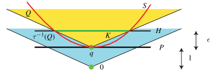
Figure 1. Flowing S backward

Let $q$ be a point in the interior of $S$. We can choose coordinates in ${\mathbb{R}}^{n+1}$ so that $S$ is tangent at $q=(1,0,\cdots,0)=e_{1}$ to the hyperplane $P$ given by $x_{1}=1$ and $S$ lies on the opposite side of $P$ to $0$.

The sublevel set $W=f^{-1}(-\infty,0]=\cup_{t\leq 0}\Phi_{t}(S)\subset{\mathcal{C}}$ is obtained by flowing $S$ backward. Let $H$ be the hyperplane $x_{1}=1+\epsilon$. Refer to Figure 1. We do not know that $S$ is properly embedded in ${\mathbb{R}}^{n+1}$. However if $\epsilon>0$ is small enough we can work in a chart for a small neighborhood of $\operatorname{dev}^{-1}(q)$ in $\xi\widetilde{M}$ and see that $K=H\cap W$ is a compact convex set and $\partial K=H\cap S$.

Let $Q$ be the convex cone consisting of the set of rays starting at $q$ and intersecting $K$. Since $q\in\partial W=S$ and $W$ is convex it follows that $Q$ contains the subset of $W$ above $H$. Unit vertical translation upwards $\tau:{\mathbb{R}}^{n+1}\to{\mathbb{R}}^{n+1}$ is given by $\tau(x)=x+e_{1}$. Note that $\tau(Q)\subset Q$. Since we can assume $\epsilon<1$ it follows that $\tau(S)$ is above $H$, therefore $Q$ contains $\tau(S)$. Hence $\tau^{-1}(Q)$ contains $S$. Since $\tau^{-1}(Q)$ is the cone from $0$ of $\tau^{-1}(K)$, it is preserved by $\Phi$ so it contains the entire orbit $\Phi\cdot S={\mathcal{C}}$. It follows that $\Omega=\pi_{\xi}({\mathcal{C}})\subset{\mathbb{RP}}^{n}$ is contained in $\pi_{\xi}(\tau^{-1}(K))$. Since $\tau^{-1}(K)$ is a compact convex set in $x_{n}=\epsilon$ it follows that $\Omega$ is properly convex. ∎

4. The Characteristic Convexity Function

In this section $V={\mathbb{R}}^{n+1}$ and $\Omega\subset\mathbb{S}(V)=\SS^{n}$ is an open properly convex set. The open convex cone ${{\mathcal{C}}}\Omega\subset V$ consists of all $t\cdot v$ with $v\in\Omega$ and $t>0$. The dual cone ${{\mathcal{C}}}\Omega^{*}\subset V^{*}$ is the set of all $\phi\in V^{*}$ with $\phi(x)>0$ for all $x\in{{\mathcal{C}}}\overline{\Omega}$. The dual domain is $\Omega^{*}={\mathbb{P}}({\mathcal{C}}\Omega^{*})\subset{\mathbb{P}}(V^{*})$. The characteristic function ${\mathchoice{\raisebox{0.0pt}{$\displaystyle\chi$}}{\raisebox{0.0pt}{$\textstyle\chi$}}{\raisebox{0.0pt}{$\scriptstyle\chi$}}{\raisebox{0.0pt}{$\scriptscriptstyle\chi$}}}={\mathchoice{\raisebox{0.0pt}{$\displaystyle\chi$}}{\raisebox{0.0pt}{$\textstyle\chi$}}{\raisebox{0.0pt}{$\scriptstyle\chi$}}{\raisebox{0.0pt}{$\scriptscriptstyle\chi$}}}_{{}_{\Omega}}:{{\mathcal{C}}}\Omega\longrightarrow{\mathbb{R}}^{+}$ of Koecher [24] and Vinberg [39] is defined by

$${\mathchoice{\raisebox{0.0pt}{$\displaystyle\chi$}}{\raisebox{0.0pt}{$\textstyle\chi$}}{\raisebox{0.0pt}{$\scriptstyle\chi$}}{\raisebox{0.0pt}{$\scriptscriptstyle\chi$}}}(x)=\int_{{{\mathcal{C}}}\Omega^{*}}e^{-\psi(x)}d\psi$$

where $d\psi$ is a fixed choice of Euclidean volume form on $V^{*}$. This function is real analytic, non-negative, and ${{\mathchoice{\raisebox{0.0pt}{$\displaystyle\chi$}}{\raisebox{0.0pt}{$\textstyle\chi$}}{\raisebox{0.0pt}{$\scriptstyle\chi$}}{\raisebox{0.0pt}{$\scriptscriptstyle\chi$}}}}(tx)=t^{-(n+1)}{\mathchoice{\raisebox{0.0pt}{$\displaystyle\chi$}}{\raisebox{0.0pt}{$\textstyle\chi$}}{\raisebox{0.0pt}{$\scriptstyle\chi$}}{\raisebox{0.0pt}{$\scriptscriptstyle\chi$}}}(x)$ for $t>0$. More generally, if $A$ is in the subgroup $\operatorname{GL}({{\mathcal{C}}}\Omega)\subset\operatorname{GL}(V)$ that preserves ${{\mathcal{C}}}\Omega,$ then ${\mathchoice{\raisebox{0.0pt}{$\displaystyle\chi$}}{\raisebox{0.0pt}{$\textstyle\chi$}}{\raisebox{0.0pt}{$\scriptstyle\chi$}}{\raisebox{0.0pt}{$\scriptscriptstyle\chi$}}}(Ax)=(\det A)^{-1}{\mathchoice{\raisebox{0.0pt}{$\displaystyle\chi$}}{\raisebox{0.0pt}{$\textstyle\chi$}}{\raisebox{0.0pt}{$\scriptstyle\chi$}}{\raisebox{0.0pt}{$\scriptscriptstyle\chi$}}}(x)$. The level sets of ${\mathchoice{\raisebox{0.0pt}{$\displaystyle\chi$}}{\raisebox{0.0pt}{$\textstyle\chi$}}{\raisebox{0.0pt}{$\scriptstyle\chi$}}{\raisebox{0.0pt}{$\scriptscriptstyle\chi$}}},$ called characteristic hypersurfaces, are smooth, convex, and meet each ray in ${{\mathcal{C}}}\Omega$ once transversely. The characteristic section is the map $\sigma_{{}_{\Omega}}:\Omega\longrightarrow{{\mathcal{C}}}\Omega$ given by

$$\sigma_{{}_{\Omega}}(x)=x\cdot({\mathchoice{\raisebox{0.0pt}{$\displaystyle\chi$}}{\raisebox{0.0pt}{$\textstyle\chi$}}{\raisebox{0.0pt}{$\scriptstyle\chi$}}{\raisebox{0.0pt}{$\scriptscriptstyle\chi$}}}(x))^{1/(n+1)}$$

It has image the characteristic hypersurface $S_{\Omega}={\mathchoice{\raisebox{0.0pt}{$\displaystyle\chi$}}{\raisebox{0.0pt}{$\textstyle\chi$}}{\raisebox{0.0pt}{$\scriptstyle\chi$}}{\raisebox{0.0pt}{$\scriptscriptstyle\chi$}}}^{-1}(1)$. The radial flow $\Phi_{t}(x)=e^{-t}\cdot x$ on $V$ preserves ${{\mathcal{C}}}\Omega$ and there is a flow function on ${{\mathcal{C}}}\Omega$ given by

$$\operatorname{c}=\operatorname{c}_{{}_{\Omega}}=(n+1)^{-1}\log{\mathchoice{\raisebox{0.0pt}{$\displaystyle\chi$}}{\raisebox{0.0pt}{$\textstyle\chi$}}{\raisebox{0.0pt}{$\scriptstyle\chi$}}{\raisebox{0.0pt}{$\scriptscriptstyle\chi$}}}$$

The Hessian $D^{2}c$ is a positive definite quadratic form at each point of ${{\mathcal{C}}}\Omega$ and gives a complete metric on ${{\mathcal{C}}}\Omega$. Thus $\operatorname{c}_{{}_{\Omega}}:{\mathcal{C}}\Omega\to{\mathbb{R}}$ is a complete convexity function called the characteristic convexity function. References for the above are Goldman [18], and [17].

If $\Gamma\subset\operatorname{SL}_{\pm}({\mathcal{C}}\Omega)$ is the holonomy of a properly convex manifold $M=\Omega/\Gamma$ with developing map $\operatorname{dev}$, then $\xi M$ is identified with ${{\mathcal{C}}}\Omega/\Gamma$. Since $c_{{}_{\Omega}}$ is preserved by $\Gamma$ it covers a map $c_{\operatorname{dev}}=c_{{}_{M}}:\xi M\to{\mathbb{R}}$. This is a convexity function for $M$ called the characteristic convexity function for $M$.

Definition 4.1.

The subspace ${\mathcal{D}ev}_{c}(M)\equiv\mathcal{D}ev_{c}(M,\mathbb{P}_{+})\subset\mathcal{D}ev(M,\mathbb{P}_{+})$ consists of the developing maps of properly convex structures for which $\partial M$ is strictly-convex.

Proof of (0.2) when $M$ is closed..

Suppose $M$ is properly convex with holonomy $\rho$ and $c_{M}:\xi M\to{\mathbb{R}}$ is a characteristic convexity function. If $\rho^{\prime}$ is close to $\rho$ then, by (1.2), there is a radiant affine manifold $N_{1}$ with holonomy $\rho^{\prime}$ and a diffeomorphism $f:\xi_{1}M\to N_{1}$ that is close to an affine map. Taking infinite cyclic covers gives a map $F:\xi M\to N$ that is close to affine. The hypersurface $S=c^{-1}(0)\subset\xi M$ maps to a hypersurface in $N$. Since $S$ is compact, Hessian-convex, and transverse to the radial flow, if $F$ is close enough in $C^{2}(\xi M,N)$ to affine, then $F(S)\subset N$ is Hessian-convex, and transverse to the radial flow $\Phi_{N}$ on $N$. This section of the radial flow defines a convexity function on $N$ by (3.3). This convexity function is complete because $N_{1}$ is compact and every Riemannian metric on a compact manifold is complete. It follows from (3.4) that $N/\Phi_{N}$ is properly convex.∎

From here until (4.2) we allow $\Omega$ to have boundary $\partial\Omega$ that is an open subset of ${\operatorname{Fr}}(\Omega)$. Let ${\mathfrak{C}}$ be the set of closed subsets of $\SS^{n}$ equipped with the Hausdorff topology. Let ${\mathcal{P}}$ be the set of properly convex $n$–manifolds $\Omega\subset\SS^{n}$ with (possibly empty) strictly-convex boundary. There is an injective map $\iota:{\mathcal{P}}\to{\mathfrak{C}}\times{\mathfrak{C}}$ defined by $f(\Omega)=({\rm cl}(\Omega),{\rm cl}(\partial\Omega))$. The Hausdorff boundary topology on ${\mathcal{P}}$ is the subspace topology given by this embedding. Thus a neighborhood of $\Omega$ consists of all $\Omega^{\prime}\in{\mathcal{P}}$ close to $\Omega$ such that $\partial\Omega^{\prime}$ is also close to $\partial\Omega$. This topology is given by a metric.

Definition 4.2.

The strong geometric topology on ${\mathcal{D}ev}_{c}(M)$ is the smallest refinement of the geometric topology such that the map ${\mathcal{D}ev}_{c}(M)\to{\mathcal{P}}$ given by $\operatorname{dev}\mapsto\operatorname{Im}(\operatorname{dev})$ is continuous.

If $M$ is closed, the strong geometric topology equals the geometric topology because fixed points of elements of the holonomy are dense in $\partial\operatorname{Im}(\operatorname{dev})$. In general two developing maps are close in this topology if they are close in the $C^{\infty}$ topology on a large compact set in the universal cover of the interior and, in addition, their images are close in the above sense. This can be expressed more simply using basepoints in the space of developing maps as in (1.3):

Suppose $\operatorname{dev}_{\rho}\in\mathcal{D}ev_{c}(M)$ and $\rho=\mathcal{H}ol(\operatorname{dev}_{\rho})$ and $\Gamma=\rho(\pi_{1}M)\subset\operatorname{SL}{{}_{\pm}}(n+1,{\mathbb{R}})$ and $\Omega_{\rho}=\operatorname{Im}(\operatorname{dev}_{\rho})\subset\SS^{n}$. Choosing $\operatorname{dev}_{\rho}$ as a basepoint means: replace $M$ by $\Omega_{\rho}/\Gamma$. Thus $\operatorname{dev}_{\rho}=i:\widetilde{M}\hookrightarrow\SS^{n}$ is now the inclusion. Then $\operatorname{dev}_{\sigma}\in{\mathcal{D}ev}_{c}(M)$ is close to $\operatorname{dev}_{\rho}$ in the strong geometric topology means: the restrictions of $\operatorname{dev}_{\sigma}$ and $i$ are close in $C^{\infty}_{w}(\operatorname{int}(\widetilde{M}),\SS^{n})$ and $\Omega_{\sigma}=\operatorname{Im}(\operatorname{dev}_{\sigma})$ is close to $\Omega_{\rho}$ in ${\mathcal{P}}$.

There is a similar notion for the radiant affine manifolds. The radiant affine manifold $N={\mathcal{C}}\Omega_{\rho}/\Gamma$ is ${\mathbb{L}}$-equivalent to $\xi M_{\rho}$. The developing map for $N$ is the inclusion $i=\operatorname{dev}_{\rho}^{\xi}:{\mathcal{C}}_{\rho}\Omega\hookrightarrow{\mathbb{R}}^{n+1}$ and $\operatorname{dev}_{\rho}^{\xi}\in\mathcal{D}ev(N,{\mathbb{L}})$. A nearby developing map $\operatorname{dev}^{\xi}_{\sigma}\in\mathcal{D}ev(N,{\mathbb{L}})$ in the strong geometric topology means: the restrictions of $\operatorname{dev}^{\xi}_{\sigma}$ and $i$ are close in $C^{\infty}_{w}(\operatorname{int}({\mathcal{C}}\Omega_{\rho}),{\mathbb{R}}^{n+1})$ and in addition ${\mathcal{C}}\Omega_{\sigma}$ is close to ${\mathcal{C}}\Omega_{\rho}$ in ${\mathcal{P}}$.

Let ${\mathcal{P}}^{\prime}\subset{\mathcal{P}}$ be the subspace of open properly convex sets. For $K\subset V$ define ${\mathcal{P}}^{\prime}(K)=\{\Omega\in{\mathcal{P}}^{\prime}\ :\ K\subset{\mathcal{C}}\Omega\ \}$. The map ${\mathcal{P}}^{\prime}\to{\mathcal{P}}^{\prime}$ given by $\Omega\mapsto\Omega^{*}$ is continuous.

Lemma 4.3.

If $K\subset\mathbb{R}^{n+1}{\setminus 0}$ is compact, then the function $\overline{{\mathchoice{\raisebox{0.0pt}{$\displaystyle\chi$}}{\raisebox{0.0pt}{$\textstyle\chi$}}{\raisebox{0.0pt}{$\scriptstyle\chi$}}{\raisebox{0.0pt}{$\scriptscriptstyle\chi$}}}}:{\mathcal{P}}^{\prime}(K)\to C^{\infty}(K)$ defined by $\overline{{\mathchoice{\raisebox{0.0pt}{$\displaystyle\chi$}}{\raisebox{0.0pt}{$\textstyle\chi$}}{\raisebox{0.0pt}{$\scriptstyle\chi$}}{\raisebox{0.0pt}{$\scriptscriptstyle\chi$}}}}(\Omega)={\mathchoice{\raisebox{0.0pt}{$\displaystyle\chi$}}{\raisebox{0.0pt}{$\textstyle\chi$}}{\raisebox{0.0pt}{$\scriptstyle\chi$}}{\raisebox{0.0pt}{$\scriptscriptstyle\chi$}}}_{{}_{\Omega}}|K$ is continuous.

Proof.

Since both topologies are metrizable it suffices to show that the image of a convergent sequence converges. Suppose the sequence $\Omega_{k}\in{\mathcal{P}}^{\prime}(K)$ converges to $\Omega_{\infty}\in{\mathcal{P}}^{\prime}(K)$, and denote the respective characteristic functions by ${\mathchoice{\raisebox{0.0pt}{$\displaystyle\chi$}}{\raisebox{0.0pt}{$\textstyle\chi$}}{\raisebox{0.0pt}{$\scriptstyle\chi$}}{\raisebox{0.0pt}{$\scriptscriptstyle\chi$}}}_{k}$ and ${\mathchoice{\raisebox{0.0pt}{$\displaystyle\chi$}}{\raisebox{0.0pt}{$\textstyle\chi$}}{\raisebox{0.0pt}{$\scriptstyle\chi$}}{\raisebox{0.0pt}{$\scriptscriptstyle\chi$}}}_{\infty}$. Define the smooth function $h:V\times V^{*}\longrightarrow{\mathbb{R}}$ by $h(x,\phi)=\exp(-\phi x)$. Then for $x\in K$, if $\partial^{\alpha}$ is an $n$’th order mixed partial derivative on $V$, then $\partial^{\alpha}h(x,\phi)=p(\phi)h(x,\phi)$ where $p(\phi)$ is a monomial of degree $n$ in the coordinates of $\phi$. Let $U=\Omega_{\infty}^{*}\ \Delta\ \Omega_{k}^{*}$ be the symmetric difference then

$$|\partial^{\alpha}{\mathchoice{\raisebox{0.0pt}{$\displaystyle\chi$}}{\raisebox{0.0pt}{$\textstyle\chi$}}{\raisebox{0.0pt}{$\scriptstyle\chi$}}{\raisebox{0.0pt}{$\scriptscriptstyle\chi$}}}_{\infty}(x)-\partial^{\alpha}{\mathchoice{\raisebox{0.0pt}{$\displaystyle\chi$}}{\raisebox{0.0pt}{$\textstyle\chi$}}{\raisebox{0.0pt}{$\scriptstyle\chi$}}{\raisebox{0.0pt}{$\scriptscriptstyle\chi$}}}_{k}(x)|\leq\int_{{{\mathcal{C}}}U}|p(\phi)h(x,\phi)|d\phi.$$

Since $K\subset{{\mathcal{C}}}(\Omega_{k}\cap\Omega_{\infty})$ it follows that $\phi(x)>0$ for all $x\in K$ and $\phi\in{\mathcal{C}}U$. Now $p(\phi)$ is polynomial in $\phi$, and $h(x,\phi)$ is exponential in $\phi$, so $p(\phi)h(x,\phi)\to 0$ exponentially fast as $\phi\to\infty$ in ${{\mathcal{C}}}U$. It follows that if $U$ is small enough, then $|\partial^{\alpha}{\mathchoice{\raisebox{0.0pt}{$\displaystyle\chi$}}{\raisebox{0.0pt}{$\textstyle\chi$}}{\raisebox{0.0pt}{$\scriptstyle\chi$}}{\raisebox{0.0pt}{$\scriptscriptstyle\chi$}}}_{\infty}-\partial^{\alpha}{\mathchoice{\raisebox{0.0pt}{$\displaystyle\chi$}}{\raisebox{0.0pt}{$\textstyle\chi$}}{\raisebox{0.0pt}{$\scriptstyle\chi$}}{\raisebox{0.0pt}{$\scriptscriptstyle\chi$}}}_{k}|<\epsilon$ on $K$. See (I.3.1) of Faraut and Korányi [16] for more details. ∎

It follows that nearby properly convex manifolds (without boundary) have nearby characteristic convexity functions:

Lemma 4.4.

Suppose $\partial M=\emptyset$. The map $\mathcal{D}ev_{c}(M)\to C^{\infty}_{w}(\xi M)$ given by $\operatorname{dev}\mapsto c_{\operatorname{dev}}$ is continuous. Here, the strong geometric topology is used on $\mathcal{D}ev_{c}(M).$

Proof.

If $\operatorname{dev},\operatorname{dev}^{\prime}\in\mathcal{D}ev_{c}(M)$ are close in the strong geometric topology then $\Omega^{\prime}=\operatorname{Im}(\operatorname{dev}^{\prime})$ is close to $\Omega=\operatorname{Im}(\operatorname{dev})$ in ${\mathcal{P}}$. By (4.3) the restrictions to $K$ of ${\mathchoice{\raisebox{0.0pt}{$\displaystyle\chi$}}{\raisebox{0.0pt}{$\textstyle\chi$}}{\raisebox{0.0pt}{$\scriptstyle\chi$}}{\raisebox{0.0pt}{$\scriptscriptstyle\chi$}}}_{\Omega}$ and ${\mathchoice{\raisebox{0.0pt}{$\displaystyle\chi$}}{\raisebox{0.0pt}{$\textstyle\chi$}}{\raisebox{0.0pt}{$\scriptstyle\chi$}}{\raisebox{0.0pt}{$\scriptscriptstyle\chi$}}}_{\Omega^{\prime}}$ are close. Composing with $\log$ shows that $c_{\Omega}$ and $c_{\Omega^{\prime}}$ are close on $K$. Thus the characteristic convexity functions $c_{\operatorname{dev}}$ and $c_{\operatorname{dev}^{\prime}}$ are close. ∎

We wish to give universal bounds on the derivatives of certain real-valued functions defined on radiant affine manifolds of the form $N={{\mathcal{C}}}\Omega/\Gamma$. If $M$ is a smooth manifold and $f\in C^{\infty}(M)$ is a smooth function, then the $k$-th derivative $D^{k}f_{x}$ at $x\in M$ is a symmetric $k$-linear map on the vector space $V=T_{x}M$ (an element of $\operatorname{Hom}(\operatorname{Sym}^{k}(V),{\mathbb{R}})$). Given a norm on $V$ we get an operator norm $\|D^{k}f_{x}\|$ defined as the infimum of $K$ for which $|D^{k}f_{x}(v_{1},\cdots,v_{k})|\leq K\|v_{1}\|\cdots\|v_{k}\|$. In our case $M={{\mathcal{C}}}\Omega$ is properly convex, and hence a Finsler manifold using the Hilbert metric on ${\mathcal{C}}\Omega$. This gives a norm $\|\cdot\|_{{\mathcal{C}}\Omega}$ called the Hilbert-Finsler norm on the tangent space to ${{\mathcal{C}}}\Omega$. There is a corresponding operator norm. The group $\operatorname{GL}({\mathcal{C}}\Omega)$ acts by isometries of this norm, which therefore pushes down to a norm on the tangent space of $N={\mathcal{C}}\Omega/\Gamma$.

Given a point $x\in{{\mathcal{C}}}\Omega$ there is a Benzécri chart $\tau$ for ${{\mathcal{C}}}\Omega$ (see 9.1) centered on $x$. This chart determines a Euclidean metric $d_{E}$ on ${{\mathcal{C}}}\Omega$, and there is also the Hilbert metric $d_{H}=d_{{{\mathcal{C}}}\Omega}$. There is a constant $K>0$ depending only on dimension such that in the ball of $d_{H}$-radius $1$ around $x$ we have $K^{-1}\cdot d_{E}\leq d_{H}\leq K\cdot d_{E}$.

It follows that universal bounds on operator norms using the Hilbert metric give bounds in the Euclidean metric for Benzécri coordinates, and vice-versa. Thus we may regard these universal bounds as bounds on ordinary partial derivatives of functions defined in a small neighborhood of the origin in ${\mathbb{R}}^{n}$ by means of Benzécri coordinates. We now use Benzécri’s compactness theorem (9.2) with (4.3) to provide uniform bounds on various properties of characteristic functions.

The restriction of the Hessian metric $D^{2}c$ to the characteristic hypersurface $S=S_{\Omega}$ is a Riemannian metric that is preserved by $\operatorname{SL}_{\pm}({\mathcal{C}}\Omega)$. If $M=\Omega/\Gamma$ is a properly convex manifold, then radial projection gives a natural identification ${\widetilde{M}}\equiv S$ and this puts a Riemannian metric on $M$ called the induced metric. The following seems to be folklore:

Corollary 4.5 (bounded curvature).

For each dimension $n>0$ there is $k_{n}>0$ such that if $M$ is a properly convex projective manifold of dimension $n$, then all sectional curvatures $\kappa$ of the induced metric on $M$ satisfy $|\kappa|<k_{n}$. Moreover the induced metric is $k_{n}$-biLipschitz equivalent to the Hilbert metric, and is therefore complete.

Proof.

If the first assertion is false there is a sequence $M_{k}=\Omega_{k}/\Gamma_{k}$ and a point $x_{k}\in M_{k}$ and a sectional curvature $\kappa>k$ at $x_{k}$. By Benzécri compactness (9.2) we may assume these domains are in Benzecri position (9.1) with $x_{k}=0$ and $\Omega_{k}\to\Omega_{\infty}$. The sectional curvature is given by a function that is a formula involving various partial derivatives of the flow function $c$. By (4.3) these functions converge to some (finite) sectional curvature for $M_{\infty}$, a contradiction. This also proves the biLipschitz result. ∎

Lemma 4.6 (uniform Hessian-convexity).

For each dimension $n$ there is ${\kappa=\kappa(n)>0}$ with the following property. Suppose $\Omega\subset{\mathbb{R}}P^{n}$ is open and properly convex and $c:{{\mathcal{C}}}\Omega\longrightarrow{\mathbb{R}}$ is the characteristic convexity function. Then $D^{2}\operatorname{c}\geq\kappa\|\cdot\|_{{\mathcal{C}}\Omega}^{2}$ everywhere.

Proof.

Since $\operatorname{c}$ is preserved by each element of $\operatorname{GL}({{\mathcal{C}}}\Omega)$ up to adding a constant, it suffices to show there is $\kappa$ such that the result holds at the center of every Benzécri domain $\Omega=\SS^{n}\cap{\mathcal{C}}\Omega$. The set of all such domains is compact (9.2), and by (4.3) the characteristic function varies smoothly with the Benzécri domain, so the result follows. ∎

If $f:(-\epsilon,\epsilon)\to{\mathcal{C}}\Omega$ is an arc parameterized by arc length then $(c\circ f)^{\prime\prime}$ is a second directional derivative. The conclusion can be rephrased as $(c\circ f)^{\prime\prime}\geq\kappa$ for every second directional derivative. We will abuse notation and write this as $c^{\prime\prime}\geq\kappa$.

Suppose $B$ is a properly convex submanifold of a properly convex manifold $M$, both without boundary, then $\xi B\subset\xi M$. The next result says that far inside $B$ the characteristic convexity functions for $B$ and $M$ are almost equal.

Lemma 4.7 (convexity functions on submanifolds).

Given $\epsilon>0$ and a dimension $n,$ there is $R=R(\epsilon,n)>0$ with the following property. Suppose $B\subset M$ are properly convex $n$–manifolds with characteristic convexity functions $c_{B}$ and $c_{M}$. Let $U\subset B$ be the subset of all $x$ with $d_{M}(x,M\setminus B)>R$ and define $g=c_{M}-c_{B}:\xi U\to{\mathbb{R}}$. Then $\|D^{k}g\|<\epsilon$ for $0\leq k\leq 2$.

Proof.

Let $\Omega_{U}\subset\Omega_{B}\subset\Omega_{M}\subset\SS^{n}$ be images of the developing maps of $U\subset B\subset M$ respectively. Since $g$ is constant along rays from the origin in ${{\mathcal{C}}}\Omega_{U}$ it suffices to show the bounds hold for $x\in\Omega_{U}:=\SS^{n}\cap{\mathcal{C}}\Omega_{U}$. Choose a Benzécri chart for $\Omega_{M}$ centered on $x$. In this chart the Euclidean distance between $\partial\Omega_{M}$ and $\partial\Omega_{B}$ is bounded above by a function $f(R)$ independent of $\Omega_{M}$ and $\Omega_{B}$ and $f(R)\to 0$ as $R\to\infty$. The result now follows using (9.2) and (4.3). ∎

5. Deforming Properly Convex Manifolds rel ends

In this section we prove a version of (1.7) for convex manifolds. We show that the only obstruction to deforming a properly convex manifold is whether the ends have such a deformation. Suppose $M_{\rho}$ is a properly convex manifold with holonomy $\rho$. The main result of this section (5.8) is that for representations $\sigma$ sufficiently close to $\rho$, if the ends of $M_{\rho}$ can be deformed to properly convex manifolds with holonomy the restriction of $\sigma$, then these deformations can be extended to all of $M_{\rho}$ to give a properly convex structure $M_{\sigma}$.

Definition 5.1.

A Finsler manifold $M=\Omega/\Gamma$ has controlled ends if there is a smooth proper function, called an exhaustion function, $f:M\to[0,\infty)$ and $K>0$ such that $\|Df\|,\|D^{2}f\|<K$ in the Finsler norm.

For example every finite volume complete hyperbolic manifold has controlled ends. If $C\cong\partial C\times[0,\infty)$ is a horocusp in a hyperbolic manifold $M$ then the horofunction $f(x)=d_{M}(x,\partial C)$ is an exhaustion function. A similar construction works on a generalized cusp (6.30). There are complete Riemannian manifolds with no exhaustion function. However:

Proposition 5.2.

Every properly convex manifold has controlled ends.

Proof.

By (4.5) every properly convex manifold admits a complete Riemannian metric that is biLipschitz equivalent to the Hilbert metric and which has bounded sectional curvature. It is a result of Schoen and Yau [33] (see also Tam [37] and Proposition 26.49 in Chow et al. [10]) that a complete Riemannian manifold of bounded sectional curvature has a proper function with bounded gradient and Hessian. ∎

Definition 5.3.

A localization function on a Finsler manifold $M$ is a smooth function $\lambda:M\to[0,1]$ with compact support and $\|D\lambda\|,\|D^{2}\lambda\|\leq 1$.

Corollary 5.4.

If $M$ is a properly convex manifold and $X\subset M$ is compact, then there is a localization function $\lambda$ on $M$ with $\lambda(X)=1$.

Proof.

By (5.2) there is an exhaustion function $f:M\rightarrow[0,\infty)$. By multiplying $f$ by a small positive scalar we may assume $\|Df\|,\|D^{2}f\|<1$ and that $f(X)\subset[0,1]$. Let $\beta:{[0,\infty)}\rightarrow[0,1]$ be a smooth function with compact support and $\beta({t})=1$ for all ${t}\leq 1$, and $\|\beta^{\prime}(t)\|,\|\beta^{\prime\prime}(t)\|\leq 1/10$ for all $t$. Then $\lambda=\beta\circ f$ has compact support and $\lambda(X)=1$. By the chain rule $\|D\lambda\|,\|D^{2}\lambda\|\leq 1$. ∎

Suppose $M=A\cup{\mathcal{B}}$ is a connected $n$–manifold and $A$ is a compact submanifold with $\partial A=\partial M\sqcup\partial{\mathcal{B}}$ and $\mathcal{B}$ has $k$ components $B_{i}$ with $1\leq i\leq k$ such that $B_{i}=\partial{B_{i}}\times[0,\infty)$. By (1.6) there is a relative holonomy map

$$\operatorname{\mathcal{E}}_{\mathbb{P}}:\mathcal{D}ev(M,\mathbb{P})\to\mathcal{R}el\mathcal{H}ol(M,\mathcal{B},\mathbb{P})$$

The subspace $\mathcal{D}ev_{c}(M,\mathbb{P})\subset\mathcal{D}ev(M,\mathbb{P})$ consists of the developing maps of properly convex structures for which $\partial M$ is strictly-convex. The subspace $\mathcal{R}el\mathcal{H}ol_{e}(M,\mathcal{B},\mathbb{P})\subset\mathcal{R}el\mathcal{H}ol(M,\mathcal{B},\mathbb{P})$ consists of the data for which each $B_{i}$ is properly convex, and $\partial B_{i}$ is strictly-convex. Then $\mathcal{D}ev_{e}(M,\mathbb{P})=\operatorname{\mathcal{E}}_{\mathbb{P}}^{-1}\mathcal{R}el\mathcal{H}ol_{e}(M,\mathcal{B},\mathbb{P})$ consists of developing maps for which these ends are properly convex with strictly-convex boundary. Finally $\mathcal{D}ev_{ce}(M,\mathbb{P})=\mathcal{D}ev_{c}(M,\mathbb{P})\cap\mathcal{D}ev_{e}(M,\mathbb{P})$ is the subspace of developing maps for properly convex structures on $M$, with $\partial M$ strictly-convex, and for which each $B_{i}$ is properly convex, and $\partial B_{i}$ is strictly-convex. The following is well known for manifolds of negative sectional curvature, cf (2.3) in Baker and Cooper [1].

Lemma 5.5.

Suppose $M$ is a properly convex real projective manifold, possibly with boundary, and $B\subset M$ is a properly convex submanifold. Then $B$ is $\pi_{1}$-injective in $M$.

Proof.

The holonomy for $B$ is injective because $B$ is properly convex. The holonomy for $B$ factors through the holonomy for $M$, therefore the map induced by inclusion $\pi_{1}B\to\pi_{1}M$ is injective. ∎

Theorem 5.6.

$\operatorname{\mathcal{E}}_{{}_{\mathbb{P}}}:\mathcal{D}ev_{ce}(M,\mathbb{P})\to\mathcal{R}el\mathcal{H}ol_{e}(M,\mathcal{B},\mathbb{P})$ is open using the geometric topology on the domain and the strong geometric topology on the codomain.

Proof.

Initially assume $M$ has no boundary. Given a developing map in $\mathcal{D}ev_{ce}(M,\mathbb{P})$ the first step is to show a nearby relative holonomy is given by a nearby (possibly not convex) projective structure that has the given end data. Then this structure is shown to be properly convex.

By (5.5) each component of $\mathcal{B}$ is $\pi_{1}$-injective in $M$. It then follows from (1.7) that $\operatorname{\mathcal{E}}_{{}_{\mathbb{P}}}:\mathcal{D}ev(M,\mathbb{P})\to\mathcal{R}el\mathcal{H}ol(M,\mathcal{B},\mathbb{P})$ is open using the geometric topologies in domain and codomain. Hence the restriction $\operatorname{\mathcal{E}}_{{}_{\mathbb{P}}}:\mathcal{D}ev_{e}(M,\mathbb{P})\to\mathcal{R}el\mathcal{H}ol_{e}(M,\mathcal{B},\mathbb{P})$ is also open with these topologies. Thus it is open using the strong geometric topology (which is finer than the geometric topology) on the codomain and the geometric topology on the domain. The end geometric topology on $\mathcal{D}ev_{e}(M,\mathbb{P})$ is defined to be the smallest refinement of the geometric topology such that $\operatorname{\mathcal{E}}_{{}_{\mathbb{P}}}$ is continuous. Then $\operatorname{\mathcal{E}}_{{}_{\mathbb{P}}}$ is open and continuous with the end geometric topology on the domain and the strong geometric topology on the codomain. This completes the first step.

As usual we will assume that ${\mathcal{B}}=B$ is connected. It suffices to show that $\mathcal{D}ev_{ce}(M,\mathbb{P})$ is open in $\mathcal{D}ev_{e}(M,\mathbb{P})$ with respect to the end geometric topology. A neighborhood $\mathcal{U}\subset\mathcal{D}ev_{e}(M,\mathbb{P})$ of $\operatorname{dev}_{\rho}$ in this topology consists of all developing maps $\operatorname{dev}_{\sigma}$ that are nearby in $C^{\infty}_{w}(\widetilde{M},{\mathbb{RP}}^{n})$ and in addition have the property that $\operatorname{dev}_{\sigma}(\widetilde{B})$ is close to $\operatorname{dev}_{\rho}(\widetilde{B})$ in ${\mathcal{P}}$.

Suppose $\operatorname{dev}_{\rho}\in\mathcal{D}ev_{ce}(M,\mathbb{P})$ has holonomy $\rho$ and $\operatorname{dev}_{\sigma}\in\mathcal{U}$ has holonomy $\sigma$. The corresponding projective structures (charts) on $M$ are denoted by $M_{\rho}$ and $M_{\sigma}$. We must show $\operatorname{dev}_{\sigma}\in\mathcal{D}ev_{c}(M,\mathbb{P})$. To do this we construct a complete convexity function on the tautological bundle $\xi M_{\sigma}$. It then follows that $M_{\sigma}$ is properly convex by (3.4).

In this sketch various manifolds should be replaced by the corresponding tautological line bundles, but for ease of exposition we do not do this. There are convexity functions for $M_{\rho}$ and $B_{\sigma}$. If $\rho$ is close to $\sigma$ then there is a diffeomorphism $M_{\rho}\rightarrow M_{\sigma}$ that is close to the identity over a large compact set $K$ whose complement is far out in the cusp $B$. The convexity function on $M_{\sigma}$ is obtained by using the one for $M_{\rho}$ over most of $K$, and the one for $B_{\sigma}$ outside $K$. We slowly transition from one function to the other over $\partial K\times[0,1]$ using a localization function to give a convex combination that changes in the $[0,1]$ direction. This ends the sketch.

We will use $M_{\rho}$ as a basepoint for ${\mathcal{D}ev}_{c}(M)$ as in (1.3), see also (4.2). Thus we replace $M$ by $M_{\rho}$ and will usually omit the subscript $\rho$. Then $\widetilde{M}=\Omega_{\rho}\subset\SS^{n}$ and $\operatorname{dev}_{\rho}:\Omega_{\rho}\hookrightarrow\SS^{n}$ is the inclusion map. Similarly we use $\xi M:={\mathcal{C}}\Omega_{\rho}/\Gamma$ as a basepoint for $\mathcal{D}ev(\xi M_{\rho},{\mathbb{L}})$ and write this as $\mathcal{D}ev(\xi M,{\mathbb{L}})$. Then $\xi\widetilde{M}_{\rho}={\mathcal{C}}\Omega_{\rho}\subset{\mathbb{R}}^{n+1}$.

We use the Hilbert-Finsler norm $\|\cdot\|$ on $\xi M$ to calculate operator norms. Recall $\xi_{1}M=\xi M/\Phi_{1}$ is the tautological circle bundle and has an infinite cyclic cover $\xi M$. Let $\kappa=\kappa(\dim(M))>0$ be the lower bound on the Hessian of characteristic functions given by (4.6) and $\epsilon=\kappa/10$. Let $R=R(\epsilon,\dim(\xi M))$ be the constant given by (4.7) and $K\subset M$ a compact connected submanifold such that $\xi_{1}K$ contains the $R$-neighborhood of $\xi_{1}A$ in $\xi_{1}M$. Hence the characteristic functions $c_{\rho,B}$ and $c_{\rho,M}$ are $\epsilon$–close in $C^{2}(\xi(M\setminus K))$.

By (5.4) there is a localization function $\lambda:\xi_{1}M\to[0,1]$ with $\lambda(\xi_{1}K)=1$ that has support inside a compact connected submanifold $\xi_{1}L$. Define $J={\rm cl}(L\setminus K)$. Then every point in $\xi_{1}J$ is distance at least $R$ from $\partial(\xi_{1}B)$. All these submanifolds depend on the choice of $\epsilon$. Let $\widetilde{\lambda}:\xi M\to[0,1]$ be the function that covers $\lambda$. We abuse notation by writing $\widetilde{\lambda}$ as $\lambda$. Observe that $\lambda^{-1}(0,1)\subset\xi J$.

Claim 1. There is a convexity function $c:\xi M\to\mathbb{R}$ which equals $c_{\rho,M}$ on $\xi K$ and equals $c_{\rho,B}$ on $\xi(M\setminus L)$ and $D^{2}c\geq(\kappa/2)\|\cdot\|^{2}$.

Proof of Claim 1.

First blend $c_{\rho,M}$ and $c_{\rho,B}$ inside $\xi J$ using $\lambda$ to get $f:\xi M\to{\mathbb{R}}$ given by

$$f=\lambda\cdot c_{\rho,M}+(1-\lambda)\cdot c_{\rho,B}=c_{\rho,M}+(1-\lambda)\cdot g$$

where $g=c_{\rho,B}-c_{\rho,M}$. The map $f$ is well defined even though $c_{\rho,B}$ is only defined on $\xi B$ because $(1-\lambda)=0$ outside $\xi B$.

Subclaim: $D^{2}f\geq(\kappa/2)\|\cdot\|^{2}$. Outside $\xi J$ this follows from (4.6) since $f=c_{\rho,M}$ on $\xi K$, and $f=c_{\rho,B}$ on $\xi(M\setminus L)$. On $\xi J$ we show this using directional derivatives. By the product rule

$$f^{\prime\prime}=c^{\prime\prime}_{\rho,M}+g^{\prime\prime}-(\lambda^{\prime\prime}g+2\lambda^{\prime}g^{\prime}+\lambda g^{\prime\prime}).$$

Since $M_{\rho}$ is properly convex $c^{\prime\prime}_{\rho,M}\geq\kappa$ by (4.6). Also $|\lambda|,|\lambda^{\prime}|,|\lambda^{\prime\prime}|\leq 1$ because $\lambda$ is a localization function and $|g|,|g^{\prime}|,|g^{\prime\prime}|<\epsilon=\kappa/10$ on $\xi J$ by definition of $R$ and $K$, so

$$|\ g^{\prime\prime}-(\lambda^{\prime\prime}g+2\lambda^{\prime}g^{\prime}+\lambda g^{\prime\prime})\ |\leq 5\epsilon=\kappa/2.$$

Thus $f^{\prime\prime}\geq\kappa/2$ which proves the subclaim. The level set $S=f^{-1}(0)$ is Hessian-convex in the backward direction of the flow and is the $0$-set of a unique flow function $c$ which coincides with $c_{\rho,B}$ outside $\xi L$. It follows from (3.3) that $c^{\prime\prime}\geq\kappa/2$ also. This proves claim 1. ∎

To avoid a proliferation of notation, and because what we are about to do is similar to what we just did, we reuse notation as follows. We define the new $K$ to be the old $L$, and the new $\lambda$ is a localization function on $\xi_{1}M$ with $\lambda(\xi_{1}K)=1$, and the new $L\subset M$ is a compact connected manifold so that $\xi_{1}L$ contains the support of $\lambda$. Then redefine $J={\rm cl}(L\setminus K)$. Let $E:={\rm cl}(M\setminus K)\subset B$. Again we write the lift as $\lambda:\xi M\to{\mathbb{R}}$. There are characteristic convexity functions $c_{\rho,B}:\xi B_{\rho}\to{\mathbb{R}}$ and $c_{\sigma,B}:\xi B_{\sigma}\to{\mathbb{R}}$.

Since $\xi_{1}L_{\rho}$ is compact, if $\mathcal{U}$ is small there is a diffeomorphism $H:\xi_{1}M_{\rho}\to\xi_{1}M_{\sigma}$ such that $H|\xi_{1}L_{\rho}$ is close in $C^{\infty}$ to the identity in the following sense. The map $H$ is covered by $\widetilde{H}:\xi\widetilde{M}_{\rho}\to\xi\widetilde{M}_{\sigma}$, and the restriction of $\widetilde{H}$ is close to the inclusion $\xi\widetilde{L}_{\rho}\hookrightarrow{\mathbb{R}}^{n+1}$ in $C^{\infty}_{w}(\xi\widetilde{L}_{\rho},{\mathbb{R}}^{n+1})$. The map $\widetilde{H}$ also covers a map $h:\xi M_{\rho}\to\xi M_{\sigma}$.

Set $g=(c_{\sigma,B})\circ h-c_{\rho,B}:\xi E_{\rho}\to{\mathbb{R}}$. If $\mathcal{U}$ is small enough then by (4.4) $c_{\sigma,B}$ and $c_{\rho,B}$ are close on $\xi J_{\rho}$. Since $\widetilde{H}$ is close to the identity map, and covers $h$, if follows that $\|D^{k}g\|<\epsilon$ for $k\in\{0,1,2\}$ everywhere on $\xi_{1}J_{\rho}$. Define $f:\xi M_{\rho}\to\mathbb{R}$ by

$$f=\lambda\cdot c+(1-\lambda)\cdot(c_{\sigma,B})\circ h.$$

As before this is well defined. Claim 2. $f^{\prime\prime}\geq\kappa/2$ on $\xi L_{\rho}$.

Proof of Claim 2.

When $\lambda=1$ then $f^{\prime\prime}=c^{\prime\prime}\geq\kappa/2$ by claim 1. The set where $\lambda<1$ is contained in $\xi J_{\rho}$. On $\xi J_{\rho}$ and $c=c_{\rho,B}$ so

$$f=\lambda\cdot c_{\rho,B}+(1-\lambda)\cdot(c_{\sigma,B})\circ h=c_{\rho,B}+(1-\lambda)\cdot g$$

and

$$f^{\prime\prime}=c_{\rho,B}^{\prime\prime}+g^{\prime\prime}-(\lambda^{\prime\prime}\cdot g+2\lambda^{\prime}g^{\prime}+g^{\prime\prime}).$$

Then $c_{\rho,B}^{\prime\prime}\geq\kappa/2$ by (4.6). As before $|\lambda|,|\lambda^{\prime}|,|\lambda^{\prime\prime}|\leq 1$ and by the above $|g|,|g^{\prime}|,|g^{\prime\prime}|<\epsilon$. Since $\epsilon<\kappa/10$ this proves claim 2. ∎

Since $\widetilde{H}$ is close to the inclusion in $C^{\infty}_{w}(\xi\widetilde{L}_{\rho},{\mathbb{R}}^{n+1})$ it follows that $f\circ h^{-1}$ is Hessian-convex on $\xi L_{\sigma}$. Outside this set $f\circ h^{-1}=c_{\sigma,B}$ which is Hessian-convex. This proves $f:\xi M_{\sigma}\to{\mathbb{R}}$ is Hessian-convex everywhere.

Again it follows from (3.3) that there is a Hessian-convex flow function $c_{\sigma}:\xi M_{\sigma}\to{\mathbb{R}}$ defined by $f\circ h^{-1}$. The corresponding Hessian metric on $\xi_{1}M_{\sigma}$ is complete because $\xi_{1}L_{\sigma}$ is compact so the metric is complete on $\xi_{1}L_{\sigma}$, and outside $\xi_{1}L_{\sigma}$ it is the complete metric given by the properly convex end $\xi_{1}B_{\sigma}$. It follows that the Hessian metric on $\xi M_{\sigma}$ is also complete. This completes the proof when $M$ has no boundary.

Now suppose $M$ has (compact) boundary and set $P=\operatorname{int}(M)$. Then $P$ is properly convex with a characteristic convexity function $c:\xi P_{\rho}\to{\mathbb{R}}$. The idea is to shrink $M$ a bit to obtain a submanifold $N\subset P$ with Hessian-convex boundary. The restriction to $N$ of the convexity function for $P$ can be used in the above arguments. It is a complete metric with $\partial N$ at a finite distance.

By (8.3) there is a submanifold $N\subset M$ with Hessian-convex, compact boundary such that ${\rm cl}(M\setminus N)$ is a collar of $\partial M$. The restriction of $c$ to $\xi N$ is a complete convexity function. There is a diffeomorphism $F:\xi M\to\xi N$ close to the identity in $C^{2}$ that is the identity outside a small collar of $\partial({\xi}M)$. Then $c_{\rho,M}:=(c|_{\xi N})\circ F:\xi M\to\mathbb{R}$ is a complete convexity function. The pullback of the restriction to $\xi N$ of the Hilbert metric on $\xi P$ is a complete metric on $\xi M$. The proof now proceeds as above to construct a complete convexity function on $\xi M_{\sigma}$. ∎

To apply (5.6) involves finding deformations of the cusps that are nearby in the strong geometric topology. This involves finding a diffeomorphism from the original cusp to the deformed cusp that is close to projective. To make this task easier we show such a map exists for a small deformation of the holonomy if the deformed domain is close to the original domain.

The projective Kleinian group space for a smooth manifold $M$ is

$$\mathcal{K}(M)=\{(\Omega,\rho)\ \in{\mathcal{P}}\times\operatorname{Rep}(M):\ M\ {\rm diffeomorphic\ to\ }\Omega/\rho(\pi_{1}M)\}$$

with topology given by the subspace topology of the product topology on ${\mathcal{P}}\times\operatorname{Rep}(M)$. This topology is given by a metric. If $(\Omega,\rho)\in\mathcal{K}(M)$ then $\Omega/\rho(\pi_{1}M)$ is a properly convex manifold with strictly-convex boundary. If $M$ is closed then $\rho$ determines $\Omega$. There is a natural map

$$\mathcal{K}:\mathcal{D}ev_{c}(M,\mathbb{P})\to\mathcal{K}(M)$$

given by $\mathcal{K}(\operatorname{dev})=(\operatorname{dev}(\widetilde{M}),\operatorname{hol}(\operatorname{dev}))$.

Proposition 5.7.

Suppose $M\cong\partial M\times[0,\infty)$ is a connected smooth manifold and $\partial M$ is compact. Then $\mathcal{K}$ is a continuous open map for the strong geometric topology on $\mathcal{D}ev_{c}(M,\mathbb{P})$.

Proof.

Continuity is obvious. Suppose $\operatorname{dev}_{\rho}\in\mathcal{D}ev_{c}(M,\mathbb{P})$ and $\mathcal{K}(\operatorname{dev}_{\rho})=(\Omega_{\rho},\rho)$ and that $(\Omega_{\sigma},\sigma)\in\mathcal{K}(M)$ is close. Then $Q=\Omega_{\sigma}/\sigma(\pi_{1}M)$ is a properly convex manifold. We identify $M\equiv\Omega_{\rho}/\rho(\pi_{1}M)$. It suffices to show there is a diffeomorphism $M\to Q$ which is almost a projective map between large compact sets in the interiors.

By (8.3) there is a diffeomorphism $M\cong\partial M\times[0,\infty)$ so that $\partial M\times t$ is $\operatorname{dev}_{\rho,M}$-Hessian-convex for all $0<t\leq 1$. For $k>1$ define $N=\partial M\times[1/k,k]$ and $W=\partial M\times[0,k+1]$ and ${E}=\partial M\times 1/k$. These are all compact. By (1.2) there is a $\operatorname{dev}_{\sigma,W}\in\mathcal{D}ev(W,\mathbb{P})$ with holonomy $\sigma$ that is close to $\operatorname{dev}_{\rho,M}{|W}$ over a compact set in $\widetilde{W}$ that covers $N$.

By (1.5) we may change $\operatorname{dev}_{\sigma,W}$ by a small isotopy so that there is a projective embedding $f:N\to Q$. If $\sigma$ is close enough to $\rho$ then, since the hypersurface ${E}$ is Hessian-convex for $\operatorname{dev}_{\rho,M},$ it follows that ${E}$ is also Hessian-convex for $\operatorname{dev}_{\sigma,W}$. Hence $f({E})$ is Hessian-convex in $Q$.

Let $P$ be the closure of the component of $Q\setminus f(N)$ that contains $\partial Q$. Since $\partial M$ is compact, for homology reasons $f({E})$ separates $\partial Q$ from the end of $Q$, thus $P$ is compact and $\partial P=\partial Q\sqcup f({E})$. Claim: $P$ is diffeomorphic to ${E}\times I$.

Since $E$ is $\operatorname{dev}_{\sigma,N}$-Hessian-convex there is a nearest point retraction (using the Hilbert metric on $Q$) $r:P\to{E}$ with fibers that are lines, and this gives a homeomorphism $P\to{E}\times I$. By [40] smooth manifolds are PL. The $M\times I$ theorem, Hirsch and Mazur [23], says that if $M$ is a PL manifold, then every smoothing of $M\times I$ is diffeomorphic to a product. Thus $P$ is diffeomorphic to $E\times I$, which proves the claim.

It follows that $P$ is a collar of $\partial Q$ so $R=P\cup f(N)\cong{E}\times[0,k]$ is also a collar of $\partial Q$. Thus $Q^{\prime}={\rm cl}(Q\setminus R)$ is diffeomorphic to ${E}\times[k,\infty)$. Clearly $P$ lies in a small neighborhood of $\partial Q$. We can now extend $f$ to a diffeomorphism $f:M\to Q$ by sending $\partial M\times[0,1/k]$ to $P$ and $\partial M\times[k,\infty)$ to $Q^{\prime}$. This is close to a projective map on $N$. Define $\operatorname{dev}_{\sigma,M}:\widetilde{M}\to{\mathbb{RP}}^{n}$ by $\operatorname{dev}_{\sigma,M}=\operatorname{dev}_{\sigma,Q}\circ\widetilde{f}$. Since $f$ is close to projective over $N$ it follows that $\operatorname{dev}_{\sigma,M}$ is close to $\operatorname{dev}_{\rho,M}$. ∎

Suppose $M=A\cup\mathcal{B}$ is a smooth manifold with (possibly empty) boundary and $A$ is a compact submanifold of $M$ with $\partial A=\partial M\sqcup\partial\mathcal{B}$. Suppose $\mathcal{B}=B_{1}\sqcup\cdots\sqcup B_{k}$ has $k$ connected components, and $B_{i}\cong\partial B_{i}\times[0,\infty)$. Define the Kleinian relative-holonomy space

(1) $$\mathcal{R}el\mathcal{H}ol(M,\mathcal{B},\mathcal{K})\subset\operatorname{Rep}(\pi_{1}M)\times\prod_{i=1}^{k}\mathcal{K}(B_{i})$$

to be the subset of all $(\rho,(\Omega_{1},\rho_{1}),\cdots,(\Omega_{k},\rho_{k}))$ such that $\rho_{i}=\rho|\pi_{1}B_{i}$. This space has the subspace topology of the product topology.

For each $B_{i}\subset M$ we fix a choice of some component $\widetilde{B}_{i}\subset\widetilde{M}$ of the preimage $B_{i}$ in the universal cover of $M$. Then $\Omega_{i}=\operatorname{dev}(\widetilde{B}_{i})$ and $\Gamma_{i}=\operatorname{hol}(\pi_{1}B_{i})$ gives a point in $\mathcal{K}(B_{i})$. This defines the Kleinian relative holonomy map

$$\operatorname{\mathcal{E}}_{\mathcal{K}}:\mathcal{D}ev_{ce}(M,\mathbb{P})\longrightarrow\mathcal{R}el\mathcal{H}ol(M,\mathcal{B},\mathcal{K})$$

Theorem 5.8 (Convex Extension Theorem).

$\operatorname{\mathcal{E}}_{\mathcal{K}}:\mathcal{D}ev_{ce}(M,\mathbb{P})\to\mathcal{R}el\mathcal{H}ol(M,\mathcal{B},\mathcal{K})$ is open using the geometric topology on the domain.

Proof.

Follows immediately from (5.6) and (5.7).∎

Proof of (0.3).

The map $\gamma:(-1,1)\to\mathcal{R}el\mathcal{H}ol(M,\mathcal{B},\mathcal{K})$ defined by

$$\gamma(t)=(\rho_{t},(\Omega_{1}(t),\rho_{t}|_{\pi_{1}B_{1}}),\cdots,(\Omega_{k}(t),\rho_{t}|_{\pi_{1}B_{k}}){)}$$

is continuous by hypothesis (5) of (0.3). By (5.8) $\operatorname{\mathcal{E}}_{\mathcal{K}}$ is open, and $\gamma(0)\in\operatorname{Im}(\operatorname{\mathcal{E}}_{\mathcal{K}})$, thus for some $\epsilon>0$ that ${\gamma}(-\epsilon,\epsilon)\subset\operatorname{Im}(\operatorname{\mathcal{E}}_{\mathcal{K}})$. So for $|t|<\epsilon$ there is $\operatorname{dev}_{t}\in\mathcal{D}ev_{ce}(M,\mathbb{P})$ with $\operatorname{\mathcal{E}}_{\mathcal{K}}(\operatorname{dev}_{t})=\gamma(t)$. Define $M_{t}$ to be the projective structure on $M$ defined by $\operatorname{dev}_{t}$. Then $M_{t}$ is properly convex, with holonomy $\rho_{t}$, and $\partial M_{t}$ is strictly-convex. Moreover the projective structure on $M_{t}$ restricted to $B_{i}$ is diffeomorphic to $P_{i}(t)$ by definition of $\operatorname{\mathcal{E}}_{\mathcal{K}}$. ∎

6. Generalized Cusps

A generalized cusp is a certain kind of properly convex projective manifold. The main result of this section is that holonomies of generalized cusps with fixed topology form an open subset in a certain semi-algebraic set (6.28). This follows from the fact that a generalized cusp contains a homogeneous cusp (6.3). We then prove the main theorem (6.29).

A cusp in a hyperbolic manifold viewed as a projective manifold is characterized by being projectively equivalent to an affine manifold that has a foliation by strictly-convex hypersurfaces that are images of horospheres, together with a transverse foliation by parallel lines. This characterization does not work in general. Consider the affine manifold $M=U/\Gamma\cong T^{2}\times[0,\infty),$ where

$$U=\{(x_{1},x_{2},x_{3}):x_{3}\geq x_{1}^{2}+x_{2}^{2}>0\ \}$$

and $\Gamma$ is the cyclic group generated by $(x_{1},x_{2},x_{3})\mapsto(2x_{1},2x_{2},4x_{3})$. It has a foliation by tori that are the images of the strictly-convex hypersurfaces $z=K(x^{2}+y^{2})$ for $K\geq 1,$ and it has a transverse foliation by vertical lines. However $M$ is not convex.

Definition 6.1.

A generalized cusp is a properly convex manifold $C=\Omega/\Gamma$ homeomorphic to $\partial C\times[0,\infty)$ with $\partial C$ a closed manifold and $\pi_{1}C$ virtually nilpotent such that $\partial\Omega$ contains no line segment, i.e. $\partial C$ is strictly-convex. The group $\Gamma$ is called a generalized cusp group.

A quasi-cusp is a properly convex manifold with interior homeomorphic to $Q\times{\mathbb{R}}$, and $Q$ is a closed manifold, and $\pi_{1}Q$ is virtually nilpotent.

If $\Gamma$ contains no hyperbolics, then $C$ is called a cusp and $\Gamma$ is conjugate to a subgroup of $PO(n,1)$ by Theorem (0.5) in [13]. An example of a quasi-cusp is $\Delta/\Gamma$ for any discrete subgroup $\Gamma\cong{\mathbb{Z}}^{n-1}$ of the diagonal group in $SL(n+1,{\mathbb{R}}),$ where $\Delta\subset{\mathbb{RP}}^{n}$ is the interior of an $n$-simplex that is preserved by $\Gamma$.

Definition 6.2.

A generalized cusp $\Omega/\Gamma$ is homogeneous if $\operatorname{PGL}(\Omega)$ acts transitively on $\partial\Omega$. The group $\operatorname{PGL}(\Omega)$ is called a (generalized) cusp Lie group.

For example a cusp in a hyperbolic manifold is homogeneous if and only if it is the quotient of a horoball $\Omega\subset\mathbb{H}^{n}$. In this case $\operatorname{PGL}(\Omega)$ is conjugate to the subgroup of $PO(n,1)\cong Isom({\mathbb{H}}^{n})$ that fixes one point at infinity. Cusp Lie groups for 3–manifolds are listed in section 7.

Theorem 6.3.

Every generalized cusp contains a homogeneous generalized cusp.

There is an equivalence relation on generalized cusps generated by the property that one cusp can be projectively embedded in another. Equivalent cusps have conjugate holonomy. One can shrink a cusp by removing a collar from the boundary. However sometimes one can remove a submanifold at the other end. For example there might be a totally geodesic codimension–1 compact submanifold in the interior of the cusp, which one could cut along. It simplifies matters to do this ahead of time.

Definition 6.4.

A generalized cusp $C$ is minimal if, for every cusp $C^{\prime}\subset C$ with $\partial C^{\prime}=\partial C$, it follows that $C=C^{\prime}$.

If $M$ is a convex manifold and $X\subset M$ then the convex hull, $\operatorname{CH}(X)$, of $X$ is the intersection of all convex submanifolds of $M$ that contain $X$. Suppose $f:S^{1}\times(-1,1]\rightarrow C$ is a diffeomorphism, and $C$ has a hyperbolic metric such that $\gamma=f(S^{1}\times 0)$ is a geodesic, and the distance $d(f(e^{i\theta},t),\gamma)=|t|$. Thus $C$ is a hyperbolic annulus with one convex boundary component, and the other boundary component deleted. Moreover $C$ is a generalized cusp, and $C^{\prime}=\operatorname{CH}(\partial C)=f(S^{1}\times{(}0,1])$ is a minimal cusp.

Lemma 6.5.

Every generalized cusp contains a unique minimal cusp. A finite cover of a minimal cusp is minimal.

Proof.

Suppose $C=\Omega/\Gamma$ is a generalized cusp. Let $\Omega^{\prime}$ be the convex hull of $\partial\Omega$. Then $\Omega^{\prime}\subset\Omega$ is properly convex and $\Gamma$-invariant and $\partial\Omega^{\prime}=\partial\Omega$. The cusp $C^{\prime}=\Omega^{\prime}/\Gamma$ is the unique minimal cusp contained in $C$. If $M$ is a finite cover of $C^{\prime}$ then $M=\operatorname{CH}(\partial M)$ so $M$ is also minimal. ∎

The following will be used frequently

Lemma 6.6.

Suppose $M$ is a quasi-cusp of dimension $n$, and $P\subset M$ is a convex submanifold, and $\pi_{1}P\rightarrow\pi_{1}M$ is an isomorphism then

• the universal cover $\widetilde{M}$ is contractible.

• $M$ is an Eilenberg-MacLane space: a $K(\pi_{1}(M),1)$.

• $H_{n-1}(\pi_{1}M;{\mathbb{Z}}_{2})\cong H_{n-1}(M;{\mathbb{Z}}_{2})\cong{\mathbb{Z}}_{2}$.

• If $\dim P<n$ then $\dim(P)=n-1$ and $P$ is a closed manifold.

• If $P\subset\operatorname{int}(M)$ and $\dim(P)<\dim(M)$ then $P$ separates.

Proof.

1,2 and 3 follow immediately from the definition. Since $P$ and $M$ are convex, they are aspherical. Hence the inclusion $P\hookrightarrow M$ is a homotopy equivalence. By (3) $H_{n-1}(P;{\mathbb{Z}}_{2})\cong{\mathbb{Z}}_{2}$ from which (4) follows.

For (5), it follows from (4) that $\dim P=n-1$. By definition of quasi-cusp, the interior of $M$ is homeomorphic to $Q\times{\mathbb{R}}$ for some closed manifold $Q$. Since $P$ and $Q$ are both closed, for sufficiently large $t\in{\mathbb{R}}$ if follows that $P$ separates $Q\times t$ from $Q\times(-t)$. ∎

By (2.1) the holonomy of a projective structure lifts to $\operatorname{GL}(n+1,\mathbb{R})$, and we will use this lift in what follows.

If $V$ is a finite dimensional vector space of dimension $n$ then a (complete) flag for $V$ is a sequence of subspaces $0=V_{0}<V_{1}\cdots<V_{n}=V$ with $\dim(V_{i})=i$. The subgroup $\operatorname{UT}(n)<\operatorname{GL}(n,{\mathbb{R}})$ consists of all upper-triangular matrices with positive diagonal entries. A group $\Gamma\subset\operatorname{GL}(n,{\mathbb{R}})$ is conjugate into $\operatorname{UT}(n)$ if and only if $\Gamma$ preserves a flag and every weight of $\Gamma$ is positive.

A connected nilpotent subgroup $\Gamma$ of $\operatorname{GL}(n,{\mathbb{C}})$ preserves a flag for ${\mathbb{C}}^{n}$. However if $\Gamma$ is not connected this need not be true. For example the quaternionic group of order $8$ in $\operatorname{GL}(2,{\mathbb{C}})$ does not preserve a flag. First we show (6.11) that there is a finite index subgroup of $\Gamma$ that preserves a flag. The index of a subgroup $H<G$ is written $|G:H|$. A subgroup $H\leq G$ is characteristic if every automorphism of $G$ preserves $H$. It is routine to show

Lemma 6.7.

$\exists\;h(n,k)>0$ such that if the group $G$ is generated by $k$ elements, then there is a characteristic subgroup $C\leq G$ with $|G:C|\leq h(n,k)$ such that if $H\leq G$ is any subgroup with index $|G:H|\leq n$ then $C\leq H$.

Suppose $V$ is a vector space over ${\mathbb{C}}$. A weight of a subgroup $\Gamma\subset\operatorname{GL}(V)$ is a homomorphism (character) $\lambda:\Gamma\rightarrow{\mathbb{C}}^{*}$ such that the weight space $E(\lambda)$ and generalized weight space $V(\lambda)$ are both non-trivial. Here,

$$E(\lambda)=\bigcap_{\gamma\in\Gamma}(\ker(\gamma-\lambda(\gamma))\quad\text{and}\quad V(\lambda)=\bigcup_{n>0}\ {\bigcap}_{\gamma\in\Gamma}(\ker(\gamma-\lambda(\gamma))^{n}.$$

A (generalized) weight space is $\Gamma$ invariant. A one-dimensional weight space is the same thing as a one-dimensional $\Gamma$–invariant subspace. The vector space $V$ has a generalized weight decomposition if $V=\oplus V(\lambda),$ where the sum is over all weights.

The group $\Gamma$ is polycyclic of (Hirsch) length (at most) $k$ if there is a subnormal series $\Gamma=\Gamma_{k}\vartriangleright\Gamma_{k-1}\cdots\vartriangleright\Gamma_{1}\vartriangleright\Gamma_{0}=1$ with $\Gamma_{i+1}/\Gamma_{i}$ cyclic for every $i$. A subgroup of a polycyclic group of length $k$ is polycyclic of length at most $k$. Every finitely-generated nilpotent group is polycyclic.

Lemma 6.8.

$\exists\;c=c(n,k)$ such that if $\Gamma<\operatorname{GL}({\mathbb{C}}^{n})$ is polycyclic of length at most $k,$ then there is a characteristic subgroup $C\leq\Gamma$ with $|\Gamma:C|\leq c$ and $C$ preserves a one-dimensional subspace of ${\mathbb{C}}^{n}$.

Proof.

We use induction on $n$ and $k$. For $n=1$ the result is obvious. For $k=1$ the result follows from Jordan normal form with $c=1$. Assume the result true for $k$. Suppose $\Gamma$ is polycyclic of length $k+1$. Then $\Gamma$ contains a normal polycyclic group $\Gamma_{k}$ of length $k$ with $\Gamma/\Gamma_{k}$ cyclic. There is a characteristic subgroup $C_{k}\leq\Gamma_{k}$ of index at most $c(n,k)$ that preserves a one-dimensional subspace $W$.

There is some weight $\lambda:C_{k}\longrightarrow{\mathbb{C}}^{*}$ with $W$ contained in the weight space $E=E(\lambda)$. There are at most $n$ weights for $C_{k}$. If $\theta$ is an automorphism of $C_{k}$ then $\lambda\circ\theta$ is a weight for $C_{k}$. Since $C_{k}$ is a characteristic subgroup of $\Gamma_{k}$, and $\Gamma_{k}$ is normal in $\Gamma$, it follows that $C_{k}$ is preserved by all inner automorphisms of $\Gamma$. Thus an inner automorphism of $\Gamma$ permutes these weights, so an element $\gamma\in\Gamma$ induces a permutation of the weights with order $m\leq n!$. Choose $\gamma\in\Gamma$ which generates $\Gamma/\Gamma_{k}$. Then $\gamma^{m}$ induces the identity permutation. Hence the subgroup $\Gamma^{\prime}=\langle C_{k},\gamma^{m}\rangle$ preserves $E$. Applying Jordan normal form to $\gamma^{m}|E$ gives a one-dimensional subspace of $E$ that is preserved by $\gamma^{m}$. This subspace is also preserved by $C_{k}$. Then $|\Gamma:\Gamma^{\prime}|\leq m|\Gamma_{k}:C_{k}|\leq n!\cdot c(n,k)$ since $m\leq n!$. By (6.7) there is a characteristic subgroup $C\leq\Gamma^{\prime}\leq\Gamma$ with $|\Gamma:C|\leq c(n,k+1)=h(n!\cdot c(n,k),k+1)$.∎

Proposition 6.9.

$\exists\;d(n,k)$ such that for all polycyclic groups $G$ of length at most $k$ there is a characteristic subgroup $C\leq G$ with $|G:C|\leq d(n,k)$ such that if $\rho:G\longrightarrow\operatorname{GL}(n,{\mathbb{C}}),$ then $\rho(C)$ preserves a flag in ${\mathbb{C}}^{n}$.

Proof.

Below we show by induction on $n$ that, for a fixed $\rho$, there is a subgroup of index at most $e(n,k)=\prod_{i=1}^{n}c(i,k)$ that preserves a flag. The result follows from (6.7) with $d(n,k)=h(e(n,k),k)$.

For $n=1$ the result is clear. By (6.8) there is a subgroup $\Gamma^{\prime}<\Gamma=\rho(G)$ of index at most $c(n,k)$ that preserves a one-dimensional subspace $E\subset V={\mathbb{C}}^{n}$. Then $\Gamma^{\prime}$ acts on $V/E\cong{\mathbb{C}}^{n-1}$. By induction there is $\Gamma^{\prime\prime}<\Gamma^{\prime}$ with $|\Gamma^{\prime}:\Gamma^{\prime\prime}|\leq e(n-1,k)$ that preserves a flag $\mathcal{F}$ in $V/E$. The preimage of $\mathcal{F}$ in $V$, together with $E$, forms a flag for $V$ which is preserved by ${\Gamma}^{\prime\prime}$. Moreover $|\Gamma:\Gamma^{\prime\prime}|=|\Gamma:\Gamma^{\prime}|\cdot|\Gamma^{\prime}:\Gamma^{\prime\prime}|\leq c(n,k)e(n-1,k)=e(n,k)$. ∎

Definition 6.10.

Suppose $G$ is a finitely-generated, virtually nilpotent group. Let $k$ the smallest integer such that $G$ is polycyclic of length $k$. Given ${n}>0$ the ${n}$–core of $G$ is the subgroup, $\operatorname{core}(G,{n})$, of $G$ that is the intersection of all subgroups of $G$ of index at most $2^{n}\cdot d({n},k)$.

Clearly $\operatorname{core}({n},G)$ is a characteristic subgroup of finite-index in $G$ that is contained in every subgroup of index at most $2^{n}$ in the subgroup $C\leq G$ from (6.9).

Corollary 6.11.

Suppose $G$ is a finitely-generated, virtually nilpotent group and $H=\operatorname{core}(G,{n})$. Then for every homomorphism $\rho:G\to\operatorname{GL}({n},{\mathbb{F}})$:

• If ${\mathbb{F}}={\mathbb{C}}$, then $\rho(H)$ preserve a flag in ${\mathbb{C}}^{n}$.

• If ${\mathbb{F}}={\mathbb{R}}$ and every weight of $\rho(H)$ is real, then $\rho(H)$ is conjugate into $UT({n})$.

• If ${\mathbb{F}}={\mathbb{R}}$ then $\rho(G)\in\operatorname{VFG}$ if and only if every weight of $\rho(H)$ is real.

• $\operatorname{VFG}(G,n)=\{\rho\in\operatorname{Hom}(G,\operatorname{GL}({n},{\mathbb{R}}))\ :\ \rho(G)\in\operatorname{VFG}\ \}$ is semi-algebraic.

Proof.

Let $C$ be the characteristic subgroup of $G$ given by (6.9). Then $H\leq C$ so (1) follows. (2) follows from (1) as follows. Set $U={\mathbb{R}}^{n}$ and $V=U\otimes{\mathbb{C}}$ so $G\subset\operatorname{GL}(U)\subset\operatorname{GL}(V)$. By (1) $V=\oplus V(\lambda)$ where $V(\lambda)=\cap_{{c\in C}}\ker(\rho({c})-\lambda({c}))^{n}$. Observe that $V(\lambda)\subset{\mathbb{C}}^{n}$ is given by linear equations that are defined over ${\mathbb{R}}$ because $\lambda({C})\subset{\mathbb{R}}$ and $\rho({C})\subset\operatorname{GL}({n},{\mathbb{R}})$. Thus $V(\lambda)$ is the complexification of $U(\lambda)=\cap_{{c\in C}}\ker(\rho({c})-\lambda({c}))^{n}\subset{\mathbb{R}}^{n}$ so $U=\oplus U(\lambda)$. Hence $\rho({C})$ preserves a flag in ${\mathbb{R}}^{n}$. By replacing $C$ by a certain subgroup, $C_{0}$, of index at most $2^{n}$ we may ensure that all real weights are positive. Since $H\leq C_{0}$ it follows that $\rho(H)$ is conjugate into $\operatorname{UT}(n)$. Clearly (2) implies (3). (4) follows from (2) and the observation that the condition that every weight is real is defined by the semi-algebraic equations that say every eigenvalue of every element of $\rho(H)$ is real. ∎

Suppose $U$ is a real vector space and $\Gamma<\operatorname{GL}(U)$ preserves a flag in $V=U\otimes{\mathbb{C}}$. Then combining each weight $\lambda$ for $V$ with the complex-conjugate weight $\overline{\lambda}$ gives a real invariant subspace $U(\lambda,\overline{\lambda})=(V(\lambda)+V(\overline{\lambda}))\cap U\subset U$ and $U=\bigoplus U(\lambda,\overline{\lambda})$. We call $U(\lambda,\overline{\lambda})$ a conjugate generalized weights space. For each $\gamma\in\Gamma$ the eigenvalues of $\gamma|_{U(\lambda,\overline{\lambda})}$ are $\lambda(\gamma)$ and $\overline{\lambda}(\gamma)$.

Proposition 6.12.

Suppose $P=\Omega/\Gamma$ is a quasi-cusp of dimension $n$. Then $\operatorname{core}(\Gamma,n+1)$ is conjugate into $\operatorname{UT}(n+1)$. In particular $\Gamma\in\operatorname{VFG}$.

Proof.

Write $V={\mathbb{R}}^{n+1}$ so $\Gamma\subset\operatorname{PGL}(V)$. By (2.1) we may lift to get $\Gamma\subset\operatorname{GL}(V)$. By (6.11)(1) we can conjugate so that $H=\operatorname{core}(\Gamma,n+1)$ is contained in the upper-triangular subgroup in $\operatorname{GL}(n+1,{\mathbb{C}})$. We replace $\Gamma$ by $H$. Then $V=A\oplus B$ where $A$ is the sum of the generalized weight spaces for real weights and $B=\oplus B_{i}$ is the sum of the remaining conjugate generalized weights spaces. It suffices to show $B=0$, since then by (6.11)(2) $\Gamma$ is conjugate into $\operatorname{UT}(n+1)$.

Each vector $x\in V$ is uniquely expressed as a linear combination $a+b_{1}+\cdots+b_{k}$ with $a\in A$ and $b_{i}\in B_{i}$. Define $n(x)$ to be the number of distinct $i$ with $b_{i}\neq 0$. Choose $x\neq 0$ with $[x]\in\Omega$ so that $n(x)$ is minimal. Claim $n(x)=0$.

Proof of the claim.

If $n(x)\neq 0,$ then some $b_{j}\neq 0$. There is $\gamma\in\Gamma$ which has eigenvalues $\lambda_{j}(\gamma),\overline{\lambda}_{j}(\gamma)$ that are not real. Let $\langle\gamma\rangle$ be the cyclic group generated by $\gamma$. Let $C\subset B_{j}$ be the convex hull of the orbit $\langle\gamma\rangle\cdot b_{j}$.

Suppose $0\notin C$. Then $K={\rm cl}({\mathbb{P}}_{+}(C))$ is a closed convex cell in ${\mathbb{P}}_{+}(B_{j})$ that is preserved by $\gamma$. By the Brouwer fixed point theorem, $\gamma$ fixes a point $[v]\in K$, so $v\in B_{j}$ is an eigenvector of $\gamma|B_{j}$ with a positive eigenvalue. However every eigenvector for $\gamma$ in $B_{j}$ has eigenvalue $\lambda_{j}(\gamma)$ or $\overline{\lambda}_{j}(\gamma)$ which are both not real. This contradiction shows that $0\in C.$

The convex cone ${{\mathcal{C}}}\Omega\subset V$ is preserved by $\Gamma$. Since $0\in C$ there is a finite convex combination $\sum t_{i}\gamma^{i}b_{j}=0$ with $t_{i}\geq 0$ and $\sum t_{i}=1$. Since $x\in{{\mathcal{C}}}\Omega$ and this cone is $\Gamma$-invariant it follows that $\gamma^{i}x\in{{\mathcal{C}}}\Omega$. Since ${\mathcal{C}}\Omega$ is convex, the convex combination $x^{\prime}=\sum t_{i}\gamma^{i}x\in{{\mathcal{C}}}\Omega$. In particular $x^{\prime}\neq 0$ and $[x^{\prime}]\in\Omega$. The component of $x^{\prime}$ in $B_{j}$ is $\sum t_{i}\gamma^{i}b_{j}=0$. Since the conjugate weights spaces are $\Gamma$ invariant, the property that a point has a zero component in some $B_{i}$ is preserved by $\Gamma$, so $n(x^{\prime})<n(x)$ contradicting minimality. Hence no such $b_{j}$ exists, and this proves the claim. ∎

Since $x\neq 0$ it follows that $A\neq 0$ and $[x]\in W:=\Omega\cap{\mathbb{P}}(A)$ is a nonempty properly convex set that is preserved by $\Gamma$. The submanifold $M=W/\Gamma$ of $P$ is convex and $\pi_{1}M\rightarrow\pi_{1}P$ is an isomorphism so $\dim(M)\geq n-1$ by (6.6). Now $B_{i}$ has real dimension at least $2$, so $\dim A\leq\dim V-\dim B_{i}\leq n-1$. But $\dim M=\dim{\mathbb{P}}(A)=\dim A-1\leq n-2$, which is a contradiction. ∎

Suppose $H$ is a Lie group. A virtual syndetic hull of a discrete subgroup $\Gamma<H$ is a connected Lie subgroup $G<H$ such that $|\Gamma:G\cap\Gamma|<\infty$ and $(G\cap\Gamma)\backslash G$ is compact. In other words $\Gamma$ is virtually a (cocompact) lattice in $H$. When syndetic hulls exist they are not always unique because the exponential map on $\mathfrak{gl}(n)$ is not injective for $n\geq 2$. It is useful to have a unique version of a syndetic hull. For more about syndetic hulls see Witte [41]. Some of the arguments that follow are inspired by section 9 of [13] which derives the classification of cusps in strictly convex projective manifolds. In particular this applies to the role of the syndetic hull.

Let $\mathfrak{r}\subset\mathfrak{gl}$ be the subset of all matrices $M$ such that all the eigenvalues of $M$ are real. The set $R=\exp(\mathfrak{r})$ consists of all matrices $A$ such that every eigenvalue of $A$ is positive. Then $\exp:\mathfrak{r}\longrightarrow R$ is a diffeomorphism with inverse $\log$. An element of $R$ is called an e-matrix, and a group $G\subset R$ is called an e-group. For example $\operatorname{UT}(n)$ is an e-group. The property of being an e-group is preserved by conjugation. If $G$ is a connected e-group, then $\exp:\mathfrak{g}\longrightarrow G$ is a diffeomorphism. If $S\subset R$ define $\langle\log S\rangle$ to be the vector subspace of $\mathfrak{gl}$ spanned by $\log S$.

Definition 6.13.

Given a discrete subgroup $\Gamma\subset\operatorname{GL}(n,{\mathbb{R}})$ a virtual e-hull for $\Gamma$ is a connected Lie group $G$ that is an e-group and $|\Gamma:G\cap\Gamma|<\infty$ and $(G\cap\Gamma)\backslash G$ is compact. There might not be such $G$.

Proposition 6.14 ((9.3) of [13]).

Suppose that $\Gamma$ is a finitely-generated, discrete nilpotent subgroup of $\operatorname{GL}(n,{\mathbb{R}})$. Then $\Gamma$ contains a subgroup of finite index $\Gamma_{0}$, which has a syndetic hull $G\leq\operatorname{GL}(n,{\mathbb{R}})$ that is nilpotent, simply-connected, and a subgroup of the Zariski closure of $\Gamma_{0}.$

Lemma 6.15.

If $\Gamma\subset\operatorname{UT}(n)$ is a finitely-generated discrete nilpotent subgroup, then it has an e-hull $G\subset\operatorname{UT}(n)$.

Proof.

By (6.14) there is a finite index subgroup $\Gamma_{0}\subset\Gamma$ which has a syndetic hull $G$. The Zariski closure of $UT(n)$ is the Borel subgroup $B$ of all upper triangular matrices in $\operatorname{GL}(n,{\mathbb{R}})$. It follows that the Zariski closure of $\Gamma$ is in $B$, so $G\subset B$. Moreover $G$ is connected so $G\subset UT(n)$. Since $\left|\Gamma:\Gamma_{0}\right|<\infty$ and $\Gamma_{0}\subset G$ it follows that $\langle\log\Gamma\rangle=\langle\log\Gamma_{0}\rangle\subset\mathfrak{g}$ thus $\Gamma\subset G$. Since $G\subset\operatorname{UT}(n)$ it is an e-group. Moreover $\Gamma\backslash G$ is a quotient of $\Gamma_{0}\backslash G$ and so is compact. Hence $G$ is a syndetic hull of $\Gamma$.∎

Lemma 6.16.

If $G_{0}$ and $G_{1}$ are virtual e-hulls of a discrete subgroup $\Gamma\subset\operatorname{GL}(n,{\mathbb{R}})$ then $G_{0}=G_{1}$.

Proof.

The group $H=G_{0}\cap G_{1}$ is connected because if $h\in H,$ then the one parameter group $\exp\langle\log h\rangle$ is contained in both $G_{0}$ and $G_{1}$. With $R$ defined above set $\Gamma^{\prime}=\Gamma\cap R$. If $\gamma\in\Gamma^{\prime}$ then $\gamma^{m}\in G_{i}$ for some ${m}>0$. Thus $\log\gamma^{m}={m}\log\gamma\in\log G_{i}$ so $\gamma\in G_{i}$. Thus $\Gamma^{\prime}=\Gamma\cap G_{i}\subset G_{i}$ so $\Gamma^{\prime}\subset H$. Since $\Gamma^{\prime}$ is a lattice in $G_{i}$, and $H$ is a closed subgroup of $G_{i}$, it follows that $\Gamma^{\prime}$ is also a lattice in $H$. Since $H$ and $G_{i}$ are diffeomorphic to their Lie algebras, if $H\neq G_{i}$ then $\dim H<\dim G_{i}$ which contradicts that $\Gamma^{\prime}$ is a lattice in $G_{i}$.∎

Definition 6.17.

If $\Gamma\subset GL(n,{\mathbb{R}})$ is finitely-generated and $\Gamma\in VFG,$ then the translation group of $\Gamma$ is $T(\Gamma)=\exp\langle\log(\operatorname{core}(\Gamma,n))\rangle$.

Theorem 6.18.

If $\Omega/\Gamma$ is a quasi-cusp then $T(\Gamma)$ is the unique virtual e-hull of $\Gamma$.

Proof.

Set $n=1+\dim\Omega$. Recall that the definition of quasi-cusp implies $\Gamma$ is virtually nilpotent. By (6.12) $\operatorname{core}(\Gamma,n)$ is conjugate into $\operatorname{UT}(n)$ and is therefore an e-group. By (6.15) $\operatorname{core}(\Gamma,n)$ has an e-hull, $T$, that is conjugate into $\operatorname{UT}(n)$. Thus $T$ is a virtual e-hull of $\Gamma$. Uniqueness of $T$ follows from (6.16). It is now clear that $T=T(\Gamma)$. ∎

The next thing to do is show that, if $\Omega/\Gamma$ is a generalized cusp of dimension $n$, the orbit under $T(\Gamma)$ of a point $x\in\partial\Omega$ is a strictly convex hypersurface. The key to doing this is to show that, if the cusp is minimal, then $\Omega$ is a closed convex subset of ${\mathbb{R}}^{n}$ bounded by $\partial\Omega$, see (6.22).

A projective flow $\Phi$ on ${\mathbb{RP}}^{n}$ is a continuous monomorphism $\Phi:{\mathbb{R}}\longrightarrow\operatorname{PGL}(n+1,{\mathbb{R}})$. There is an infinitesimal generator $A\in\mathfrak{gl}_{n+1}$ with $\Phi_{t}:=\Phi(t)=\exp(tA)$. If $p\in{\mathbb{RP}}^{n}$ and $\Phi_{t}(p)=p$ for all $t,$ then $p$ is a stationary point of $\Phi$. A radial flow is a projective flow that is stationary on a hyperplane $H\cong{\mathbb{R}}P^{n-1}$, and that is parameterized so that $\Phi_{t}(p)\to r\in H$ as $t\to-\infty$ whenever $p$ is not stationary. It follows that $\Phi_{t}=\exp(tA),$ where $A\in\mathfrak{gl}_{n+1}$ is a rank one matrix, and $H$ is the projectivization of $\ker A$. The projectivization of the image of $A$ is a point $p\in{\mathbb{R}}P^{n}$, called the center of the flow, that is also fixed by $\Phi$. Every orbit is contained in a line containing the center. This property characterizes radial flows.

A radial flow is parabolic if $p\in H$ and hyperbolic otherwise. Every radial flow is conjugate to one generated by an elementary matrix $E_{i,j}$. A parabolic flow is conjugate to $(I+t\cdot E_{1,n+1})$ and a hyperbolic flow is conjugate to the diagonal group $(\exp(t),1,\cdots,1)$. The backward orbit of $X\subset{\mathbb{RP}}^{n}$ is $\Phi_{(-\infty,0]}(X)$. A set $X\subset{\mathbb{RP}}^{n}$ is backward invariant if $X$ contains its backward orbit, and it is backward vanishing if $\cap_{t<0}\Phi_{t}(X)=\emptyset$.

A displacing hyperplane for a radial flow $\Phi$ is a hyperplane $P$ such that $P$ and $\Phi_{t}(P)$ are disjoint in ${\mathbb{RP}}^{n}\setminus H$ for all $t\neq 0$. A hyperplane $P$ is displacing if and only if $P\neq H$ and $P$ does not contain the center of $\Phi$.

Proposition 6.19.

Suppose $\Omega/\Gamma$ is a quasi-cusp and $\Gamma\subset\operatorname{UT}(n+1)$. If $\lambda:\Gamma\to{\mathbb{R}}^{*}$ is a weight with generalized weight space $V=V(\lambda)$ then there is a radial flow $\Phi=\Phi^{\lambda}$ that is centralized by $\Gamma$, and $\Phi$ acts trivially on each generalized weight space other than $V$.

If $\dim V\geq 2$, then $\Phi$ is parabolic, and if $\dim V=1,$ then $\Phi$ is hyperbolic. The center of $\Phi$ is contained in ${\mathbb{P}}(E(\lambda))$. The group $G(\Gamma):=T(\Gamma)\times\Phi({\mathbb{R}})$ generated by $T(\Gamma)$ and $\Phi({\mathbb{R}})$ is their internal direct product. If the orbit of $x\in{\mathbb{RP}}^{n}$ under $T(\Gamma)$ is a strictly-convex hypersurface then $G(\Gamma)\cdot x\subset{\mathbb{RP}}^{n}$ is open.

Proof.

We may assume $\Gamma$ is upper-triangular and block diagonal, with one block for each generalized weight space. We may assume $V$ is the first block and set $m=\dim V$. As above, let $E_{i,j}\in\mathfrak{gl}(n{+1})$ be the elementary matrix with $1$ in row $i$ and column $j$. Define $\Phi(t)=\exp(tE_{1,m})$. Then $\mathbb{R}^{n+1}=V\oplus W$ where $W$ is the sum of the other generalized weight spaces and the action of $\Phi$ on $W$ is trivial. If $m=1$ then $\Phi(t)=\operatorname{diag}(\exp(t),1,\cdots,1)$ is a hyperbolic flow. If $m\geq 2$ then $\Phi(t)$ is a parabolic flow given by the unipotent subgroup with $t$ in the top right corner of the block for $V$. The center is ${\mathbb{P}}(e_{1})$ and the stationary hyperplane is $H={\mathbb{P}}(\langle e_{1},\cdots,e_{m-1}\rangle\oplus W)$. It is easy to check that $\Gamma$ centralizes $\Phi$.

Since $T(\Gamma)=\exp(\mathfrak{t})$ and $\Phi({\mathbb{R}})=\exp(\mathfrak{f})$ are $e$-groups, if they have a nontrivial intersection, then $\Phi({\mathbb{R}})\subset T(\Gamma)$. The orbits of $\Phi$ are lines. If $S=T(\Gamma)\cdot x$ is a strictly-convex hypersurface, then it does not contain a line so $\Phi({\mathbb{R}})\cap\Gamma$ is trivial, and $\Phi({\mathbb{R}})\cdot S\subset{\mathbb{RP}}^{n}$ is open. Since $\Phi({\mathbb{R}})$ and $T(\Gamma)$ commute they generate $G=T(\Gamma)\times\Phi({\mathbb{R}})$. ∎

Definition 6.20.

A radial flow $\Phi_{t}$ is compatible with a properly convex manifold $M=\Omega/\Gamma$ if $\Phi({\mathbb{R}})$ commutes with $\Gamma$, and $\Omega$ is disjoint from the stationary hyperplane of $\Phi$, and $\Omega$ is backward invariant and backward vanishing.

A radial flow end is a properly convex manifold $M=\Omega/\Gamma$ with compact, strictly convex boundary, and for which there is a compatible radial flow. A radial flow cusp is a radial flow end that is also a generalized cusp.

The hypersurfaces $\widetilde{S}_{t}:=\Phi_{-t}(\partial\Omega)$ are strictly-convex and $\Gamma$-invariant. Those with $t\geq 0$ foliate $\Omega$. They are all disjoint from $H$. Their images under the projection $\pi:\Omega\to M$ give a product foliation of $M$ by compact, strictly-convex, hypersurfaces $S_{t}=\pi(\widetilde{S}_{t})$. There is a transverse foliation of $\Omega$ by flow-lines that limit on the center of $\Phi$. These project to a transverse foliation of $M$ by rays.

The flow time function is $\widetilde{T}:\Omega\to[0,\infty)$ defined by $\widetilde{T}(x)=t$ if $\Phi_{t}(x)\in\partial\Omega$. Thus $\widetilde{T}(x)$ is the amount of time for $x$ to flow into $\partial\Omega$ and $\widetilde{T}(\widetilde{S}_{t})=t$. Let $\pi:\Omega\to M$ be the projection. Then there is a map $T:M\to[0,\infty)$ defined by $T(\pi x)=\widetilde{T}(x)$. The level sets of $T$ are the hypersurfaces $S_{t}$.

Lemma 6.21.

Suppose $\Phi$ is a radial flow with center $p$ and stationary hyperplane $H$. Suppose $\Omega\subset{\mathbb{RP}}^{n}\setminus H$ is properly convex. If $\Phi$ is hyperbolic and $p\notin{\rm cl}(\Omega),$ then $\Omega$ is backward vanishing. If $\Phi$ is parabolic, then $\Omega$ is backward vanishing for either $\Phi(t)$ or $\Phi^{\prime}(t):=\Phi(-t)$.

Proof.

If $\Phi$ is hyperbolic and $p\notin{\rm cl}(\Omega),$ then by the Hahn-Banach separation theorem there is a hyperplane $P$ that separates $\Omega$ from $p$. If $\Phi$ is parabolic, then choose any hyperplane $P$ disjoint from $\Omega$ that does not contain $p$. In either case $P$ is a displacing hyperplane. After possibly reversing $\Phi$ in the parabolic case, the component of ${\mathbb{R}}^{n}\setminus P$ that contains $\Omega$ is a half-space that is backward vanishing, and hence so is $\Omega$. ∎

The reason for introducing radial flow ends is:

Lemma 6.22.

Suppose $\Omega\subset{\mathbb{RP}}^{n}$ and $M=\Omega/\Gamma$ is a radial flow end with radial flow $\Phi.$ Let $H\subset{\mathbb{RP}}^{n}$ be the stationary hyperplane for $\Phi$, and $\overline{\Omega}={\rm cl}(\Omega)\subset{\mathbb{RP}}^{n}$. Then $\partial\overline{\Omega}=\partial\Omega\sqcup(H\cap\overline{\Omega})$. In particular, $\Omega$ is a closed convex subset of ${\mathbb{R}}^{n}={\mathbb{RP}}^{n}\setminus H$ bounded by the properly embedded, strictly-convex hypersurface $\partial\Omega$.

Proof.

Let ${\mathbb{R}}^{n}={\mathbb{RP}}^{n}\setminus H,$ so that $\Omega\subset{\mathbb{R}}^{n}$. It suffices to show that $\partial\Omega$ is properly embedded in ${\mathbb{R}}^{n}$ and therefore $\Omega$ is a closed convex set in ${\mathbb{R}}^{n}$ bounded by $\partial\Omega$.

Let $p$ be the center of $\Phi$. Choose a displacing hyperplane $P\subset{\mathbb{RP}}^{n}$ that is disjoint from $\Omega$ such that if $\Phi$ is hyperbolic then $P$ separates $p$ from $\Omega$ in ${\mathbb{R}}^{n}$.

Let $U$ be the closure of the component of ${\mathbb{R}}^{n}\setminus P$ that is the half-space containing $\Omega.$ Then $U$ is backward invariant. Thus $U$ is the backward orbit of $P$. Define the function $\tau:U\to[0,\infty)$ by $\tau(x)=t$ if $\Phi_{t}(x)\in P$. This is the amount of time it takes $x$ to flow into $P$. Observe that if $x,y\in\Omega,$ then $\widetilde{T}(x)-\widetilde{T}(y)=\tau(x)-\tau(y)$.

Because $\widetilde{S}_{t}:=\Phi_{-t}(\partial\Omega)$ is strictly-convex, it follows that the only critical points of the restriction of $\widetilde{T}$ to a segment are maxima, and therefore there is at most one critical point on a segment. Thus $T:M\to[0,\infty)$ has the same critical point behavior along segments.

Choose a metrically-complete Riemannian metric on $M$ and use the lifted metric on $\Omega$. Suppose $\partial\Omega$ is not properly embedded in ${\mathbb{R}}^{n}$. Then there is a sequence $\widetilde{p}_{k}\in\partial\Omega$ which converges in ${\mathbb{R}}^{n}$ to a point $\widetilde{p}_{\infty}\notin\partial\Omega$.

Let $\alpha_{k}$ be the length of $[\widetilde{p}_{0},\widetilde{p}_{k}]\subset\Omega$. Then $\alpha_{k}\to\infty$ because $\widetilde{p}_{\infty}\notin\Omega$ and the metric on $\Omega$ is complete. Let $\widetilde{\ell}_{k}:[0,1]\to[\widetilde{p}_{0},\widetilde{p}_{k}]$ be the unit segment. Then $\widetilde{\ell_{k}}$ converges to $\widetilde{\ell}_{\infty}:[0,1]\to[\widetilde{p}_{0},\widetilde{p}_{\infty}]$. The restriction of $\widetilde{\ell}_{\infty}$ to $[0,1)$ is a ray, $\widetilde{\ell}:[0,1)\to\Omega$, of infinite length in $\Omega$. Since $\widetilde{p}_{k}\to\widetilde{p}_{\infty}$ there is $\beta>0$ such that ${\widetilde{T}}\circ\widetilde{\ell}_{k}\leq\beta$ for all $k\in[0,\infty]$.

The projection $\ell_{k}=\pi\circ\widetilde{\ell}_{k}:[0,1]\to M$ is an immersed affine segment and $T\circ\ell_{k}\leq\beta$. Thus $\ell_{k}$ is contained in the compact set $M_{\beta}:=\cup_{0\leq t\leq\beta}S_{t}$. These segments converge to the ray $\ell=\pi\circ\widetilde{\ell}$ of infinite length that is also contained $M_{\beta}$. Now $T\circ\ell:[0,1)\to[0,\beta]$ is eventually monotonic. Thus there is a segment, $\ell^{*}:[0,1]\to M_{\beta}$, of length $1$ that is a limit of subsegments of $\ell$ of length 1, and $T\circ\ell^{*}$ is some constant $\alpha$. Thus $\ell^{*}$ is contained in $S_{\alpha}$. But this contradicts the fact that $S_{\alpha}$ is strictly-convex. It follows that $\partial\Omega$ is properly embedded in ${\mathbb{R}}^{n}$. Hence $\Omega$ is a closed convex set in ${\mathbb{R}}^{n}$. ∎

To apply this we need

Proposition 6.23.

Every minimal generalized cusp $C=\Omega/\Gamma$ with $\Gamma\subset\operatorname{UT}(n+1)$ is a radial flow cusp.

Proof.

It suffices to show there is a radial flow that is compatible with $C$.

Claim 1. $\Omega$ is disjoint from every $\Gamma$-invariant hyperplane $H$.

Proof of claim 1.

If $H\cap\Omega\neq\emptyset$, then $H\cap\partial\Omega\neq\emptyset$ since $C$ is minimal. Observe that $H\cap\Omega$ is properly convex and preserved by $\Gamma$. Thus $R=(H\cap\Omega)/\Gamma$ is a convex codimension-1 submanifold of $C$ with nonempty boundary, which contradicts (6.6).∎

There are now two cases:

Parabolic case. There is a generalized weight space $W$ for $\Gamma$ with $\dim W\geq 2$. Let $\Phi$ be the parabolic radial flow that centralizes $\Gamma$ given by (6.19). Let $H$ be the stationary hyperplane and $p\in H$ the center of $\Phi$. Let $P$ be a displacing hyperplane that is tangent to $\Omega$ at $q\in\partial\Omega$.

Hyperbolic case. Every generalized weight space has dimension $1$, so $\Gamma$ is diagonalizable. The weight spaces projectivize to give points $p_{0},\cdots,p_{n}\in{\mathbb{RP}}^{n}$ that are in general position. The hyperplane $P_{i}$ contains all these points except $p_{i}$. These hyperplanes divide ${\mathbb{RP}}^{n}$ into $2^{n}$ open $n$-simplices. These hyperplanes are $\Gamma$-invariant so $\Omega$ is contained in one of these simplices, say $\Delta$, by minimality of the cusp. There is a vertex $p$ of $\Delta$ with $p\notin\overline{\Omega}$ because $\partial\Omega$ is a strictly-convex hypersurface in $\Delta$. After relabelling $p=p_{0}$, let $H=P_{0}$ and let $\Phi$ be the radial flow with center $p$ and stationary hyperplane $H$. Then $\Phi$ centralizes $\Gamma$ and $p$ is disjoint from ${\rm cl}(\Omega)$. By the proof of (6.21) there is a displacing hyperplane $P$ that separates $p$ from $\Omega$.

In each case, $\Omega$ is disjoint from $H$ by claim 1. Set ${\mathbb{R}}^{n}={\mathbb{RP}}^{n}\setminus H$ so $\Omega\subset{\mathbb{R}}^{n}$. Let $U$ be the closure of the component of ${\mathbb{R}}^{n}\setminus P$ that contains $\Omega$. Choose linear coordinates on ${\mathbb{R}}^{n}$ such that $q=e_{1}=(1,0,\cdots,0),$ and $U$ is the half-space $x_{1}\geq 1,$ and, moreover, $p=0$ in the hyperbolic case and $p$ is the limit of the positive $x_{1}$-axis in the parabolic case. Then $P=\partial U$ is the horizontal hyperplane $x_{1}=1$.

We may assume $U$ is backward invariant after possibly reversing the flow in the parabolic case. We reparameterize $\Phi$ so that in these coordinates, in the parabolic case $\Phi_{t}(x)=x-t\cdot e_{1}$, and in the hyperbolic case $\Phi_{t}(x)=\exp(-t)\cdot x$.

Let $p_{1}:U\to P$ be the projection along flow-lines. In the parabolic case $p_{1}(x_{1},\cdots,x_{n})=(1,x_{2},\cdots,x_{n})$ and in the hyperbolic case $p_{1}(x_{1},\cdots,x_{n})=(1,x_{2}/x_{1},\cdots,x_{n}/x_{1})$. Let $\Omega_{1}$ be the backward orbit of $\operatorname{int}\Omega$.

Claim 2. $\Omega_{1}$ is open in ${\mathbb{R}}^{n}$, properly convex, backward invariant and contains $\operatorname{int}(\Omega)$.

Proof of claim 2.

Clearly $\Omega_{1}$ is open, backward invariant, and contains $\operatorname{int}(\Omega)$. Suppose $a,b\in\Omega_{1}.$ Then $a=\Phi_{\alpha}(a^{\prime})$ and $b=\Phi_{\beta}(b^{\prime})$ for some $\alpha,\beta\leq 0$ and $a^{\prime},b^{\prime}\in\operatorname{int}\Omega$. Let $\ell=[a^{\prime},b^{\prime}]$ be the line segment with endpoints $a^{\prime},b^{\prime}$. Since $\Omega$ is convex $\ell\subset\Omega$. Then $\cup_{t\leq 0}\Phi_{t}(\ell)$ is a planar convex set in $\Omega_{1}$ that contains $a$ and $b$. Hence $\Omega_{1}$ is convex.

Let $C$ be the cone of $\Omega$ from $0$. Since $\Omega$ is properly convex, and ${0}\notin\overline{\Omega}$, it follows that $C$ is properly convex. Moreover $C$ contains $\Omega_{1}$, so $\Omega_{1}$ is properly convex, proving claim 2. ∎

We want to add a boundary to $\Omega_{1}$ and show this gives $\Omega$. Define $\Omega_{M}$ to be the flow closure of $\Omega_{1}$, i.e. the set of all points $x$ such that $\Phi_{t}(x)\in\Omega_{1}$ for all $t<0$. Clearly $\Omega_{M}\subset{\rm cl}(\Omega_{1})\subset{\mathbb{R}}^{n}$. There is a homeomorphism $\widetilde{F}:\partial\Omega_{M}\times[0,\infty)\to\Omega_{M}$ given by $F(x,t)=\Phi_{-t}(x)$. Since $\Omega_{1}$ is open, $\Omega_{M}$ is a manifold with boundary $\partial\Omega_{M}$. It is clear that $\Omega_{M}$ is disjoint from $H$, backward invariant and backward vanishing.

Claim 3. $\Gamma$ acts freely and properly discontinuously on $\Omega_{M}.$

Proof of claim 3.

Since $\Gamma$ commutes with $\Phi$ it follows that $\Omega_{1}$ is preserved by $\Gamma$. Also $\Gamma$ acts freely on $\Omega$, it contains no elliptics, and therefore acts freely on $\Omega_{1}$. By (1.3) of [13] $\Gamma$ is discrete and therefore acts properly discontinuously on $\Omega_{1}$. The map $\Phi_{-1}$ embeds $\Omega_{M}$ into $\Omega_{1}$ and, since $\Phi_{-1}$ commutes with $\Gamma$, it follows that $\Gamma$ acts freely and properly discontinuously on $\Omega_{M}$. ∎

Thus $M=\Omega_{M}/\Gamma$ is a properly convex manifold and there is a homeomorphism $F:\partial M\times[0,\infty)\to M$ covered by $\widetilde{F}$. Claim 4. $M=C$.

First we show $C\subset M$. Since $\operatorname{int}(\Omega)\subset\Omega_{1}$ it follows that $\operatorname{int}(C)\subset\operatorname{int}(M)$. By (8.3) there is a collar neighborhood $P\subset C$ of $\partial C$ with $\partial P=\partial C\sqcup Q$ and $Q$ is strictly-convex. Let $R={\rm cl}(C\setminus P)$ so $\partial R=Q$ and $R$ is a generalized cusp contained in $M$. Thus $X={\rm cl}(M\setminus R)\cong\partial X\times I$ is a compact, and $P\setminus\partial C\subset X,$ so it follows that $\partial C{\subset X}\subset M$, thus $C\subset M$.

The intersection of an orbit under the flow $\Phi$ with $\Omega_{M}$, and also its image in $M$, is called a flow-line. Every flow-line $\lambda$ in $M$ ends on $\partial M$ and is properly embedded. Moreover $C\cap\lambda$ is convex. Since $\partial C$ separates $\partial M$ from the end of $M$, it follows that $\lambda\cap C$ is all of $\lambda$ except, possibly, a bounded interval at the end of $\lambda.$ It follows that for all $t<0$ that $\Phi_{t}(C)\subset C$ so $C$ is backward invariant. It now follows that $\Omega_{1}=\Omega$ and $M=C$, and this implies $\Phi$ is compatible with $C$. ∎

Now we know that $\Omega$ is a closed subset of ${\mathbb{R}}^{n}$ we are ready to show the orbits of the translation group are properly embedded convex hypersurfaces in ${\mathbb{R}}^{n}$.

Proposition 6.24.

Suppose $C=\Omega/\Gamma$ is a minimal generalized cusp and $\Gamma\subset\operatorname{UT}(n+1)$. Let $T=T(\Gamma)$ be the translation group. Then $C$ contains a minimal homogeneous cusp $C_{T}=\Omega_{T}/\Gamma$ and $T$ acts transitively on $\partial\Omega_{T}$.

Proof.

By (6.23) $C$ is a radial flow cusp for some flow $\Phi$. Let $H$ be the stationary hyperplane of $\Phi$ and set ${\mathbb{R}}^{n}={\mathbb{RP}}^{n}\setminus H$. Since $T$ centralizes $\Phi$, it preserves $H$, and acts affinely on ${\mathbb{R}}^{n}$. Claim. There is $x\in\Omega$ such that $T\cdot x\subset\Omega$.

Proof of claim.

Let $\pi:\Omega\longrightarrow C$ be the covering space projection. There is a continuous map $F:T\times\partial\Omega\to{\mathbb{R}}^{n}/\Gamma$ given by $F(t,x)=\pi(t\cdot x)$. Since $\partial C=\partial\Omega/\Gamma$ is compact, there is a compact subset $D\subset\partial\Omega$ such that $\Gamma\cdot D=\partial\Omega.$ So $T\cdot\partial\Omega$=$T\cdot D$ because $\Gamma\subset T$. There is compact $X\subset T$ such that $\Gamma X=T.$ So $T\cdot D=(\Gamma X)\cdot D$. Hence $\operatorname{Im}(F)=\pi(X\cdot D)$ because $\pi(\Gamma\cdot x)=\pi(x)$. Thus ${K=}\operatorname{Im}(F)\subset{\mathbb{R}}^{n}/\Gamma$ is compact, because it equals $F(X\times D)$, and $X\times D$ is compact. Choose $x\in\operatorname{int}(\Omega)$ such that $\pi(x)\notin K$. Then $T\cdot x$ is connected, and disjoint from $\partial\Omega$. By (6.22) $\operatorname{int}(\Omega)\subset\mathbb{R}^{n}$ is bounded by $\partial\Omega$. It follows that $T\cdot x\subset\Omega$. This proves the claim. ∎

The set $\Omega_{T}={\rm cl}(\operatorname{CH}(T\cdot x))\subset\Omega$ is properly convex and $T$–invariant. Claim $\partial\Omega_{T}$ is strictly convex. Since $\Omega_{T}$ is a closed properly convex set in ${\mathbb{R}}^{n}$, there is an extreme point $y\in\partial\Omega_{T}$ at which $\partial\Omega_{T}$ is strictly-convex. Thus $\partial\Omega_{T}$ is strictly-convex at every point in the orbit $S=T\cdot y\subset\partial\Omega_{T}$. Then $\Omega_{S}:=\operatorname{CH}(S)\subset\Omega_{T}$ is properly convex. Since $\Gamma\subset T$ it follows that $\Omega_{S}$ is $\Gamma$-invariant. Thus $C_{S}=\Omega_{S}/\Gamma$ is a generalized cusp and a submanifold of $C$. It follows from (6.6) that $\dim\Omega_{S}=\dim\Omega$. Moreover $S\subset\partial\Omega_{T}$ so $S\subset\partial\Omega_{S}$. Since $\Omega_{S}=CH(S)$ it follows that $S=\partial\Omega_{S}{=\partial\Omega_{T}}$ and $\Omega_{S}=\Omega_{T}$, which proves the claim. ∎

If $\Omega/\Gamma$ is a generalized cusp, by (6.24) there is a homogeneous domain $\Omega_{T}\subset\Omega$ that is preserved by the finite index subgroup of $\Gamma\cap T(\Gamma)$. Next we show that $\Omega_{T}$ is preserved by all of $\Gamma$.

Lemma 6.25.

Suppose $C=\Omega/\Gamma$ is a minimal generalized cusp and $T=T(\Gamma)\subset\operatorname{UT}(n+1)$ and $\Gamma_{0}=T\cap\Gamma$. Suppose $\Omega/\Gamma_{0}$ contains a homogeneous cusp $\Omega_{T}/\Gamma_{0}$ and $\Omega_{T}$ is preserved by $T$. Then $\Gamma$ preserves $\Omega_{T}$ so $C$ contains the homogeneous generalized cusp $\Omega_{T}/\Gamma$.

Proof.

By (6.23) $C^{*}=\Omega_{T}/\Gamma_{0}$ is a radial flow cusp and by (6.22) $\Omega_{T}\subset{\mathbb{R}}^{n}$ is bounded by the strictly-convex properly embedded hypersurface $\partial\Omega_{T}$. By (6.18) $T=T(\Gamma)$ is the unique translation group that contains $\Gamma$.

Since $\Gamma$ normalizes itself it follows that $\Gamma$ normalizes $T$ and therefore $\Gamma$ permutes the decomposition of ${\mathbb{RP}}^{n}$ into $T$–orbits. The domain $\Omega_{T}$ is foliated by $T$–orbits and $\Omega_{T}/T\cong[0,1)$. Since $\Gamma\cap T$ preserves $\Omega_{T}$ and $|\Gamma:\Gamma\cap T|<\infty$ it follows the $\Gamma$–orbit of $\Omega_{T}$ is a finite number of pairwise disjoint convex sets all contained in $\Omega$. Thus $\Gamma\cap T$ permutes these domains. There is a finite index subgroup $\Gamma_{1}\subset\Gamma\cap T$ that preserves each domain. We may assume $\Gamma_{1}$ is normal in $\Gamma$. Thus $M=\Omega/\Gamma_{1}$ is a regular cover of $C$ that contains one copy of $P=\Omega_{T}/\Gamma_{1}$ for each domain. However $M$ and each copy of $P$ is a generalized cusp. Each copy of $\partial P$ separates $\partial M$ from the end of $M$. Since the copies of $P$ are disjoint there is only one copy of $P$ and $\Gamma$ preserves $\Omega_{T}$. ∎

Proof of (6.3).

Suppose $C=\Omega/\Gamma$ is a generalized cusp of dimension $n$. We may assume $C$ is minimal by (6.5). Since $\Gamma$ is virtually nilpotent, it follows from (6.12) there is a finite index subgroup $\Gamma^{\prime}<\Gamma$ that is conjugate into $\operatorname{UT}(n+1)$. We will assume this conjugacy has been done. Then $\widetilde{C}=\Omega/\Gamma^{\prime}$ is a generalized cusp that is a finite cover of $C$ and is minimal by (6.5). It follows from (6.18) that $\Gamma^{\prime}$ is a lattice in a connected upper-triangular Lie group $T=T(\Gamma)$. By (6.23) it follows that $\widetilde{C}$ is a radial flow cusp for a radial flow $\Phi$ with stationary hyperplane $H$. Let ${\mathbb{R}}^{n}={\mathbb{RP}}^{n}\setminus H.$ By (6.22) $\Omega\subset{\mathbb{R}}^{n}$ is a closed strictly-convex set bounded by the strictly-convex hypersurface $\partial\Omega$. By (6.24) there is a properly convex $\Omega_{T}\subset\Omega$ that is $T$-invariant and thus $\Gamma^{\prime}$-invariant. By (6.25) $\Omega_{T}$ is preserved by all of $\Gamma$ hence $\Omega_{T}/\Gamma$ is a homogeneous cusp in $C$ and $\Gamma<\operatorname{PGL}(\Omega_{T})$. ∎

Lemma 6.26.

Suppose $G$ is a connected group with $\dim G=n-1$. For $x\in{\mathbb{RP}}^{n}$ the subset of $\operatorname{Hom}(G,\operatorname{GL}(n+1,{\mathbb{R}}))$ consisting of all $\rho$ with $\rho(G)\cdot x$ a Hessian convex hypersurface is open.

Proof.

Suppose the map $f:G\longrightarrow{\mathbb{RP}}^{n}$ given by $f(g)=(\rho(g))\cdot x$ has image a strictly-convex hypersurface $S$. Because $G$ acts transitively on $S$ by projective maps it follows that $S$ is strictly-convex everywhere if and only if it is strictly-convex at the single point $x$. Let $\nu$ be the normal to $S$ at $x$, and $e\in G$ the identity. Hessian convexity of $S$ at $x$ is equivalent to the quadratic form $Q=\nu\cdot D^{2}_{e}f$ being positive or negative definite. This form $Q=Q(\rho)$ is a smooth function of $\rho$, and the set of definite quadratic forms is open in the set of all quadratic forms. ∎

Definition 6.27.

If $C$ is a generalized cusp of dimension $n$, then $\mathcal{GC}(C)$ is the subspace of $\operatorname{Hom}(\pi_{1}C,\operatorname{GL}(n+1,{\mathbb{R}}))$ consisting of holonomies of all generalized cusp structures on $C$, and $\operatorname{VFG}({C})$ is the subspace of all $\rho$ with $\rho(\pi_{1}{C})\in\operatorname{VFG}$

Theorem 6.28 (stability of generalized cusps).

Suppose ${C}$ is a generalized cusp of dimension $n$. Then

• $\operatorname{VFG}({C})$ is semi-algebraic.

• $\mathcal{GC}(C)\subset\operatorname{VFG}(C).$

• $\theta:\mathcal{K}({C})\rightarrow\operatorname{VFG}({C})$ given by $\theta(\Omega,\rho)=\rho$ is a continuous open map.

• $\mathcal{GC}(C)=\operatorname{Im}(\theta)$.

Proof.

By (6.11) $\operatorname{VFG}({C})$ is semi-algebraic. By definition $(\Omega,\rho)\in\mathcal{K}({C})$ if and only if $\Omega/\operatorname{Im}(\rho)$ is a generalized cusp diffeomorphic to ${C}$, thus $\mathcal{GC}(C)=\operatorname{Im}(\theta)$. Every generalized cusp is homogeneous by (6.3), and (6.12) implies the holonomy contains a finite index subgroup that is conjugate into an upper triangular group, so $\mathcal{GC}(C)\subset\operatorname{VFG}({C})$. It is obvious that $\theta$ is continuous, it only remains to show it is open.

Set $H=\operatorname{core}(\pi_{1}{C},n+1)$. By (6.17) , given $(\Omega,\rho)\in\mathcal{K}({C})$ the translation group is

$$T(\rho):=T(\rho(\pi_{1}{C}))=\exp\langle\log(\rho H)\rangle.$$

This is clearly a continuous function of $\rho$.

Choose $x\in\partial\Omega$. By (6.26) for $\sigma\in\operatorname{VFG}({C})$ close enough to $\rho$ the hypersurface $S=T(\sigma)\cdot x$ is Hessian convex, and close to $\partial\Omega$. By (6.19) there is a radial flow $\Phi$ that is centralized by $T(\sigma)$ and the group $G=T(\sigma)\oplus\Phi({\mathbb{R}})$ has an open orbit $W$ in ${\mathbb{RP}}^{n}$. Moreover $W$ is foliated by the strictly-convex hypersurfaces $S_{t}=\Phi_{t}(S)$.

After replacing $t$ by $-t$ we may assume for $t<0$ and close to $0$ that $S_{t}$ is on the convex side of $S=S_{0}$. Let $\Omega^{+}=\cup_{t\leq 0}S_{t}.$ Then $\partial\Omega^{+}=S_{0}$. This set is preserved by $T(\sigma)$ and therefore by $\sigma(H)$. It is contained in a properly convex cone by the argument of (3.4) using Figure 1. Hence $\Omega(\sigma):=\operatorname{CH}(\Omega^{+})$ is properly convex and $T(\sigma)$–invariant. The argument of claim 3 in (6.23) shows that $\sigma(H)$ acts freely and properly discontinuously on $\Omega(\sigma)$. Since $\Omega(\sigma)$ is $T(\sigma)$–invariant, $\partial\Omega(\sigma)$ is Hessian convex. Thus $\Omega(\sigma)/\sigma(H)$ is a homogeneous generalized cusp.

It only remains to show that $\Omega(\sigma)$ is preserved by all of $\sigma(\pi_{1}{C})$. The argument is very similar to the proof of (6.25). The $\sigma(\pi_{1}{C})$–orbit of $\Omega(\sigma)$ is finite because $|\pi_{1}{C}M:H|<\infty$. By (6.16) $T(\sigma)$ is the unique virtual e-hull of $\sigma(\pi_{1}{C})$. Thus $\sigma(\pi_{1}{C})$ preserves the decomposition of ${\mathbb{RP}}^{n}$ into $T(\sigma)$–orbits. Moreover $\Omega(\sigma)$ is a union of such orbits. Thus if $g\in\pi_{1}{C}$ then $(\sigma g)(\Omega(\sigma))$ is either $\Omega(\sigma)$ or disjoint from $\Omega(\sigma)$. We need only look at finitely many such $g$. Observe that $\Omega(\sigma)$ is close to $\Omega(\rho)$ and $\rho(g)$ is close to $\sigma(g)$ and $\rho(\pi_{1}{C})$ preserves $\Omega(\rho).$ Thus $\rho(g)$ preserves $\Omega(\rho)$ so $(\sigma g)(\Omega(\sigma))$ intersects $\Omega(\sigma)$. It follows that $(\sigma g)(\Omega(\sigma))=\Omega(\sigma)$. ∎

We remark that when ${C}\cong T^{2}\times[0,\infty)$ the subset of diagonal representations in $\operatorname{GL}(3,{\mathbb{R}})$ given by holonomies of generalized cusps is not closed. The boundary consists of properly convex structures on ${C}$ with $\partial{C}$ flat, thus not strictly-convex.

Theorem 6.29 (Main Theorem).

Suppose $N$ is a compact connected $n$–manifold and $\mathcal{V}=\cup_{i=1}^{k}V_{i}\subseteq\partial N$ is the union of some of the boundary components of $N.$ Assume $\pi_{1}V_{i}$ is virtually nilpotent for each $i$. Let $M=N\setminus\mathcal{V}$. Then the holonomy map $\mathcal{H}ol:\mathcal{D}ev_{ce}(M)\to\operatorname{VFG}(M)$ is continuous and open, and $\operatorname{VFG}(M)$ is a semi-algebraic subset of $\operatorname{Hom}(\pi_{1}M,\operatorname{GL}(n+1,{\mathbb{R}}))$.

Proof.

Continuity is obvious. That $\operatorname{VFG}(M)$ is semi-algebraic follows from (6.11). Let $B_{i}$ be the end of $M$ corresponding to $V_{i}$ and $\mathcal{B}=\cup B_{i}$. Given a developing map $\operatorname{dev}\in\mathcal{D}ev_{ce}(M)$ the holonomy $\rho=\mathcal{H}ol(\operatorname{dev})\in\operatorname{VFG}(M)$ by (6.12). The restriction $(\operatorname{dev}|B_{i})$ determines a generalized cusp $B_{i}\cong\Omega_{i}/\Gamma_{i}$ with holonomy $\Gamma_{i}=\rho(\pi_{1}B_{i})$. If $\rho^{\prime}\in\operatorname{VFG}(M)$ is sufficiently close to $\rho$, then by (6.28) there are nearby generalized cusps $B_{i}\cong\Omega^{\prime}_{i}/\Gamma^{\prime}_{i}$ with holonomy $\Gamma^{\prime}_{i}=\rho^{\prime}(\pi_{1}B_{i})$. Thus $x=(\rho,(\Omega_{1},\Gamma_{1}),\cdots,(\Omega_{k},\Gamma_{k}))$ and $x^{\prime}=(\rho^{\prime},(\Omega_{1}^{\prime},\Gamma^{\prime}_{1}),\cdots,(\Omega^{\prime}_{k},\Gamma^{\prime}_{k}))$ are close in $\mathcal{R}el\mathcal{H}ol(M,\mathcal{B},\mathcal{K})$. By (5.8) the map

$$\operatorname{\mathcal{E}}_{\mathcal{K}}:\mathcal{D}ev_{ce}(M,\mathbb{P})\to\mathcal{R}el\mathcal{H}ol(M,\mathcal{B},\mathcal{K})$$

is open, so there is $\operatorname{dev}^{\prime}$ close to $\operatorname{dev}$ with $\operatorname{\mathcal{E}}_{\mathcal{K}}(dev^{\prime})=x^{\prime}$ and $\mathcal{H}ol(x^{\prime})=\rho^{\prime}$. Hence $\mathcal{H}ol$ is open. ∎

Proof of (0.2).

By definition $\operatorname{Rep_{ce}}(M)=\operatorname{Im}(\mathcal{H}ol)$, so the result follows from (6.29).∎

We may avoid appealing to the theorem of Schoen and Yau used in the proof of (5.2) for the manifolds appearing in the main theorem using:

Lemma 6.30.

Every homogeneous cusp has an exhaustion function.

Proof.

Suppose ${C}=\Omega/\Gamma$ is a homogeneous cusp and $T=T(\Gamma)$ is the translation subgroup. Then $\Omega$ has a codimension–1 foliation by $T$–orbits that covers a smooth foliation of ${C}$. Pick $y$ in the interior of $\Omega$ and define $F:\Omega\to\mathbb{R}$ by $F(x)=d_{\Omega}(x,T\cdot y)$ if $T\cdot y$ separates $\partial\Omega$ from $x$, and define $F(x)=0$ otherwise. Then $F$ covers a map $f:{C}\to\mathbb{R}$ and $Y=f^{-1}(0)$ is a compact collar neighborhood of $\partial{C}$ and $f(x)=d(y,Y)$ and $f^{-1}(t)$ is a leaf of the foliation of ${C}$ for $t>0$.

It is clear that $\|df\|\leq 1$ when $f>0$. Thus it suffices to show that $\|D^{2}f\|$ is bounded. Suppose there is a sequence $({C}_{k},f_{k},x_{k})$ such that $\|D^{2}f_{k}\|_{x_{k}}>k$. Then ${C}_{k}=\Omega_{k}/\Gamma_{k}$ and $\Gamma_{k}$ is a lattice in $G_{k}=\operatorname{PGL}(\Omega_{k})$. We may assume all the $\Omega_{k}$ are in Benzecri position and $0$ covers $x_{k}$. We may also assume $\Omega_{k}\to\Omega$ in the Hausdorff topology. Then $G_{k}\to G\subset\operatorname{PGL}(\Omega)$. The $T$ orbits are a smooth foliation of $\Omega$ and we define a smooth function $F:\Omega\longrightarrow\mathbb{R}$ using $y=0$ as above. Then $F_{k}$ converges to $F$ in $C^{\infty}$ on compact sets. But $\|D^{2}f_{k}\|=\|D^{2}F_{k}\|\to\infty$ contradicts $\|D^{2}F\|<\infty$ because $F$ is smooth.∎

7. Three dimensional generalized cusps

An orientable three-dimensional generalized cusp is diffeomorphic to $T^{2}\times[0,\infty)$, and Leitner [27] shows that the holonomy is conjugate into a unique group of the form below with $\beta\geq\alpha>0$ fixed, where $n$ is the number of non-trivial weights:

$$C_{0}=\begin{pmatrix}1&s&t&\frac{s^{2}+t^{2}}{2}\\ 0&1&0&s\\ 0&0&1&t\\ 0&0&0&1\end{pmatrix}\qquad C_{1}=\begin{pmatrix}e^{s}&0&0&0\\ 0&1&t&\frac{1}{2}t^{2}-s\\ 0&0&1&t\\ 0&0&0&1\end{pmatrix}$$

$$C_{2}(\alpha)=\begin{pmatrix}e^{s}&0&0&0\\ 0&e^{t}&0&0\\ 0&0&1&-t-\alpha s\\ 0&0&0&1\end{pmatrix}\qquad C_{3}(\alpha,\beta)=\begin{pmatrix}e^{s}&0&0&0\\ 0&e^{t}&0&0\\ 0&0&e^{-\alpha s-\beta t}&0\\ 0&0&0&1\end{pmatrix}$$

Figure 2. Generalized cusps in dimension $3$

A related statement, due to Benoist, is in (2.7) of [4]. There is a compact, properly convex domain $\Omega_{n}=\Omega_{n}(\alpha,\beta)$ preserved by $C_{n}=C_{n}(\alpha,\beta)$ and $\partial\Omega_{n}=A\sqcup B$ where $A=C_{n}\cdot x$ is an orbit and $B$ is a simplex contained in a projective hyperplane. If $\Gamma_{n}\subset C_{n}$ is a lattice then $\overline{M}=\Omega_{n}/\Gamma_{n}$ is a compactification of the generalized cusp $M=(\Omega_{n}\setminus B)/\Gamma_{n}$ obtained by adding $\partial_{\infty}\overline{M}=B/\Gamma$ which is a point for $C_{0}$, a circle for $C_{1}$, and a torus for $C_{2}$ or $C_{3}$. The group $C_{n}$ is a translation group and is contained in the cusp Lie group $\operatorname{PGL}(\Omega_{n})$.

The group $C_{0}$ is conjugate into $PO(3,1)$ and contains the holonomy of a cusp of a hyperbolic 3-manifold. Ballas [2] found a lattice in $C_{1}$ that is the holonomy of a generalized cusp for a properly convex structure on the figure eight knot complement. The groups $C_{3}(\alpha,\beta)$ are diagonal affine groups that satisfy the uniform middle eigenvalue condition of Choi [9]. Gye-Seon Lee found lattices in some of these groups that are holonomies of generalized cusps for a properly convex structure on the figure eight knot complement. At the time of writing it is not known if there is 3-manifold that admits a finite volume hyperbolic structure and also a properly convex structure that is a lattice in some $C_{2}(\alpha)$. The classification of generalized cusps in all dimensions is given in Ballas, Cooper and Leitner [3].

8. Convex Smoothing

We are concerned with various kinds of convexity. A function $f:(a,b)\to{\mathbb{R}}$ is convex if

$$\forall(c,d)\subset(a,b)\ \forall t\in(0,1)\quad f(tc+(1-t)d)\leq tf(c)+(1-t)f(d)$$

and strictly-convex if the above inequality is always strict. It is Hessian-convex if $f$ is smooth and $f^{\prime\prime}>0$ everywhere. A convex function is strictly-convex at $p\in(a,b)$ if the graph of $y=f(x)$ intersects the tangent line at $x=p$ at the single point $(p,f(p))$.

Each of these definitions extends to a function $f:M\to{\mathbb{R}}$ on an affine manifold $M$ by requiring its restriction to each line segment in $M$ to have the corresponding property. In the case of Hessian convex we also require $f$ is smooth. It follows that if a convex function $f:M\to{\mathbb{R}}$ is strictly-convex at the point $p\in M$, then there is hyperplane $H$ and a neighborhood $U\subset M$ of $p$ such the graph of $f|U$ intersects $H$ only at $p$. For affine manifolds, we show how to approximate a convex function which is strictly-convex somewhere by a smooth, Hessian-convex one.

The main application is that given a projective manifold which has a convex boundary that is strictly-convex at some point, we can shrink the manifold slightly to produce a submanifold with Hessian-convex boundary: locally the graph of a Hessian-convex function. One might imagine using sandpaper to smooth the boundary and produce a submanifold with smooth strictly-convex boundary.

The idea is to improve a convex function which is already Hessian-convex on some open subset, by changing it in a small convex set $C$, and leaving it unchanged outside $C$. This is done so that it is Hessian-convex inside a slightly smaller convex set $C^{-}\subset C$, and also Hessian-convex at any point where it was previously Hessian-convex. In this way the problem is reduced to a local one in Euclidean space.

Greene and Wu [21, Theorem 2], and also [20], showed that on a Riemannian manifold, any function $f$ with the property that locally there is a function $g$ with positive definite Hessian such that $f-g$ is convex along geodesics (they call $f$ strictly-convex) can be uniformly approximated by smooth, Hessian-convex functions. Smith [36] gives an example, for each $k\geq 0$, of a $C^{k}$ convex function on a non-compact Euclidean surface which is not approximated by a $C^{k+1}$ convex function.

A function $f$ is convex down if $-f$ is convex. This means secant lines lie below the graph: $tf(a)+(1-t)f(b)\leq f(ta+(1-t)b)$ for all $a,b$ and $0\leq t\leq 1$. Equivalently the set of points below the graph of $f$ is convex.

If $f,g$ are smooth convex down functions, then $\min(f,g)$ is convex down, but need not be smooth at points where $f=g$. We construct a smooth approximation $m^{\kappa}$ on ${\mathbb{R}}_{+}^{2}$ which agrees with $\min$ outside a certain neighborhood of the diagonal and has good convexity properties.

Lemma 8.1 (smoothing min).

Given $\kappa\in(0,1)$ there is a smooth function $m^{\kappa}:{\mathbb{R}}_{+}^{2}\longrightarrow{\mathbb{R}}_{+},$ which is convex-down and non-decreasing in each variable ($m^{\kappa}_{x}\geq 0,m^{\kappa}_{y}\geq 0$), such that if $x\leq\kappa y$ or $y\leq\kappa x,$ then $m^{\kappa}(x,y)=\min(x,y)$. Moreover $m^{\kappa}$ is linear along rays: $m^{\kappa}(tx,ty)=t\cdot m^{\kappa}(x,y)$ for $t\geq 0$. It follows that if $f,g:C\longrightarrow{\mathbb{R}}_{+}$ are convex down, then so is $h(x)=m^{\kappa}(f(x),g(x))$.

Proof.

On ${\mathbb{R}}_{+}^{2}$

$$\min(x,y)=(x+y)\cdot k(x/(x+y)),\qquad\text{where }k(t)=\min(t,1-t).$$

Choose $\delta$ so that $\kappa=\delta/(1-\delta).$ Then $\delta\in(0,1/2)$. Let $K:[0,1]\longrightarrow[0,1]$ be a convex-down smooth function that agrees with $k$ outside $(\delta,1-\delta)$. Define $m:{\mathbb{R}}_{+}^{2}\longrightarrow{\mathbb{R}}$ by

$$m(x,y)=(x+y)\cdot K(x/(x+y)).$$

Clearly $m$ is linear along rays. If $x/(x+y)\leq\delta,$ then $m(x,y)=x$. This happens when $x\leq\kappa y$. Similarly $m(x,y)=y$ when $y\leq\kappa x$, thus

$$m(x,y)=\min(x,y)\quad\text{if}\quad x\leq\kappa y\ \text{or\ }y\leq\kappa x.$$

The subset of ${\mathbb{R}}_{+}^{2}$ where neither $x\leq\kappa y$ nor $y\leq\kappa x$ is called the transition region. Outside the transition region $m=\min$.

The graph of $m$ is a convex-down surface above ${\mathbb{R}}^{2}_{+}$ that is a union of rays starting at the origin. One can picture the graph of $m$: it is the cone from the origin of the convex-down arch that is the part of the graph lying above $x+y=1$. This arch is given by $K(x)$. Since $K(x)$ is convex down, the graph of $m$ is convex-down; though in the radial direction it is, of course, linear.

This surface is comprised of three parts. The central part is curved down. The other two parts are sectors of flat planes, one containing the $x$–axis and the other containing the $y$–axis.

We claim $m(x,y)$ is a non-decreasing function of each variable. This is clear on the two parts of the graph of $m$ that are flat, since they are planes containing either the $x$-axis or the $y$-axis. Now

$$m_{x}(a,b)=\frac{\partial m}{\partial x}=K(a/(a+b))+(a+b)\cdot b(a+b)^{-2}K^{\prime}(a/(a+b)).$$

Since $m_{x}(ta,tb)=m_{x}(a,b)$ we may assume $a+b=1.$ Then

$$m_{x}(a,b)=K(a)+(1-a)K^{\prime}(a)=:c.$$

The point $(x,y)=(1,c)$ lies on the tangent line to the graph of $y=K(x)$ at $x=a$. Since this graph is convex down, and underneath the graph of $y=k(x)$, it follows that $c\geq 0$. This is best seen by staring at a diagram. Similar calculations work for $m_{y}$. This proves the claim.

Next we deduce that $h$ is convex-down using these two properties of $m$, where

$$h(ta+(1-t)b)=m(f(ta+(1-t)b),g(ta+(1-t)b)).$$

Since $m_{x}\geq 0$ and $f$ is convex-down

$$m(f(ta+(1-t)b),g(ta+(1-t)b))\geq m(tf(a)+(1-t)f(b),g(ta+(1-t)b))$$

Similarly $m_{y}\geq 0$ and $g$ is convex-down

$$\begin{array}[]{rcl}m(tf(a)+(1-t)f(b),g(ta+(1-t)b))&\geq&m(tf(a)+(1-t)f(b),tg(a)+(1-t)g(b))\\ &=&m(t(f(a),g(a))+(1-t)(f(b),g(b))).\end{array}$$

Finally since $m$ is convex down

$$\begin{array}[]{rcl}m(t(f(a),g(a))+(1-t)(f(b),g(b)))&\geq&t\cdot m(f(a),g(a))+(1-t)m(f(b),g(b))\\ &=&t\cdot h(a)+(1-t)h(b).{\hskip 136.5733pt\qed}\end{array}$$

Corollary 8.2 (relative convex smoothing).

Suppose $C\subset{\mathbb{R}}^{n}$ is a compact convex set with nonempty interior and $C^{-}$ is a compact convex set in the interior of $C$. Suppose $f:C\longrightarrow{\mathbb{R}}$ is a non-constant, convex function, which is Hessian-convex on a (possibly empty) subset $S\subset C$. Assume $f|\partial C=0$. Then there is a convex function $F:C\longrightarrow{\mathbb{R}}$ such that $F$ is Hessian-convex on $S\cup C^{-}$ and $f=F$ on some neighborhood of $\partial C$.

Proof.

Observe $f<0$ on the interior of $C$. Let $g$ be a Hessian-convex function on ${\mathbb{R}}^{n}$ which is negative everywhere on $C$ and $g\geq f/2$ everywhere on $C^{-}$. Since $f$ is not identically zero this can be done with, for example, $g(x)=\alpha\|x\|^{2}+\beta$ with suitable constants.

For $\kappa\in(0,1/2)$ define $F(x)=-m^{\kappa}(-f(x),-g(x))$ then $F(x)=\max(f(x),g(x))$ except when $f(x)$ is close enough to $g(x)$, depending on $\kappa$. Since $g<f=0$ on $\partial C$ it follows that $F=f$ on some neighborhood of $\partial C$. Moreover $F=g$ on $C^{-}$ and therefore $F$ is Hessian-convex on $C^{-}$.

By (8.1) $F$ is convex. Since $m=m^{\kappa}$ and $g$ are smooth and the composition of smooth functions is smooth, it follows $F$ is smooth on $S$. It only remains to show $D^{2}F$ is positive definite on $S$. It suffices to show for every $a\in S$ and every unit vector $u\in{\mathbb{R}}^{n}$ the function $p(t)=-F(a+t\cdot u)$ satisfies $p^{\prime\prime}(0)<0.$ Computing

$$p^{\prime}=-m_{x}f_{u}-m_{y}g_{u}$$

where

$$m_{x}=\frac{\partial m}{\partial x},\ m_{y}=\frac{\partial m}{\partial y}$$

and $f_{u},g_{u}$ are the derivatives in direction $u$ at $a\in C,$

$$f_{u}=df(u),\quad g_{u}=dg(u).$$

Then

$$p^{\prime\prime}=[m_{xx}(f_{u})^{2}+2m_{xy}f_{u}g_{u}+m_{yy}(g_{u})^{2}]\ -\ [m_{x}f_{uu}+m_{y}g_{uu}].$$

Since $m$ is smooth and convex down it follows that $D^{2}m$ is negative semi-definite, so the first term is $\leq 0$. By 8.1 we have $m_{x}\geq 0$ and $m_{y}\geq 0$. Also $g_{uu}>0$ everywhere and $f_{uu}>0$ on $S$. Since $m$ is linear along rays, and $m(x,y)>0$ on the positive quadrant ($x>0$ and $y>0$), it follows that $m_{x}+m_{y}>0$ on the positive quadrant, so the $m_{x}f_{uu}+m_{y}g_{uu}>0$ everywhere on $S$. Hence $p^{\prime\prime}<0$ everywhere on $S$ as required. ∎

A component $N$ of the boundary of a projective manifold $M$ is Hessian-convex if $N$ is locally the graph over the tangent hyperplane of a smooth function with positive definite Hessian in some chart.

Proposition 8.3 (smoothing convex boundary).

Suppose $M$ is a projective manifold and $\partial M$ is everywhere locally convex, and also strictly-convex at one point on each component of $\partial M$. Then there is a submanifold $N\subset M$ such that $M\setminus\operatorname{int}(N)\cong[0,1]\times\partial N$ and $\partial N$ is Hessian-convex.

Proof.

Suppose $\partial M$ is strictly-convex at $x\in\partial M$. Choose a (subset of a) hyperplane $H\subset M$ close to $x$ so that the component, $C$, of $M\setminus H$ containing $x$ is a small convex set $V$. Using local affine coordinates, $S=C\cap\partial M$ is the graph over $H$ of a convex function $f,$ which is $0$ on $H\cap\partial M$. Apply (8.2) to produce a smooth function $g$ with positive definite Hessian and satisfying $0\leq g\leq f$. The graph of $g$ is a smooth hypersurface between $H$ and $S$. Replace $S$ by this graph. This smoothes out part of $\partial M$. Repeating this procedure smoothes the entire boundary. ∎

In a similar way one can prove:

Corollary 8.4 (smoothing convex functions).

Suppose $M$ is a connected affine manifold and $f:M\longrightarrow\mathbb{R}$ is a convex function, which is strictly-convex at some point. Given $\epsilon>0$ there is $g:M\longrightarrow\mathbb{R},$ which is smooth, Hessian-convex and satisfies $|f-g|<\epsilon$.

9. Benzécri’s Theorem

Theorem 9.1 (Benzécri [5]).

For each $n>1$ there is a Benzécri constant $R=R_{\mathcal{B}}(n)\leq 5^{n-1}$ with the following property. Suppose $\Omega$ is a properly convex open subset of ${\mathbb{RP}}^{n}$ and $p\in\Omega$. Then there is a projective transformation $\tau\in\operatorname{PGL}(n+1,{\mathbb{R}})$ such that $\tau(p)=0$ and $B(1)\subset\tau(\Omega)\subset B(R),$ where $B(t)$ is the closed ball of radius $t$ in ${\mathbb{R}}^{n}$ centered at $0$.

The projective transformation $\tau$ is called a Benzécri chart for $\Omega$ centered at $p$ and the image $\tau(\Omega,p)$ is called Benzécri position. The following proof is shorter and more elementary than the traditional proof using John ellipsoids, and also provides an algorithm to find a Benzécri chart. The set of Benzécri charts for $(\Omega,p)$ is a compact subset of $\operatorname{PGL}(n+1,{\mathbb{R}})$.

Proof.

The proof is by induction on $n$. If $n=1,$ then $\Omega$ is an open interval in ${\mathbb{R}}P^{1}$ with closure a closed interval. There is a projective transformation taking $\Omega$ to $(-1,1)$ and $p$ to $0$ so $R_{\mathcal{B}}(1)=1$.

For the inductive step, choose a projective hyperplane $H^{n-1}\subset{\mathbb{RP}}^{n}$ containing $p$. Then $\Omega^{\prime}=\Omega\cap H$ is an open convex set in $H\cong{\mathbb{R}}P^{n-1}$ and $p\in\Omega^{\prime}$. Since $\Omega$ is properly convex, $\overline{\Omega}$ is disjoint from some projective hyperplane $K^{n-1}.$ Thus $\overline{\Omega}^{\prime}=\overline{\Omega}\cap H$ is disjoint from $H\cap K,$ which is a hyperplane in $H$. It follows that $\Omega^{\prime}$ is properly convex in $H$. By induction, and after choosing appropriate coordinates on an affine patch in $H$ (or using a fixed coordinate system and applying a Benzécri transformation to $\Omega^{\prime}$), we may assume that $\Omega^{\prime}\subset{\mathbb{R}}^{n-1}\times 0\subset H$ with $p=0$ and $B^{n-1}(1)\subset\Omega^{\prime}\subset B^{n-1}(r),$ where $r=R_{\mathcal{B}}(n-1)$.

Figure 3. Shadows

There are affine coordinates on ${\mathbb{RP}}^{n}\setminus K={\mathbb{R}}^{n}$ so that the affine part of $H$ is ${\mathbb{R}}^{n-1}\times 0$. In what follows we will apply projective transformations in $\operatorname{PGL}(n+1,{\mathbb{R}})$ which are the identity on $H$. This moves $\Omega$ while keeping $\Omega^{\prime}$ fixed. The first step is to arrange that

$$\Omega\subset{\mathbb{R}}^{n-1}\times[-1,1]$$

and $\partial\Omega$ contains a point $z\in{\mathbb{R}}^{n-1}\times 1$. Then we may shear so that $z=(0,\cdots,0,1)$.

Next consider the one-parameter group $A(t)\in\operatorname{PGL}(n+1,{\mathbb{R}})$ fixing $z$ and $H$. As $t$ varies, the points that are not fixed move between $z$ and $H$. This group preserves the family of affine planes $\{x_{n}=\text{const}\}$ in ${\mathbb{R}}^{n}$. Since it fixes $z$ the affine plane ${\mathbb{R}}^{n-1}\times 1$ is preserved (though not fixed) by this group. Thus we may move $\Omega$ by an element of this group so that it is still contained in ${\mathbb{R}}^{n-1}\times[-1,1]$, still contains $z$, and

$$A=\Omega\cap\big{(}{\mathbb{R}}^{n-1}\times(-1)\big{)}$$

is not empty. Let $C\subset{\mathbb{R}}^{n-1}\times[-1,1]$ be the set of points on all lines $\ell$ passing through $z$ and some point in $\Omega^{\prime}$. Then $S=C\cap[{\mathbb{R}}^{n-1}\times(-1)]$ is the shadow from the point $z$ of $\Omega^{\prime}$ on ${\mathbb{R}}^{n-1}\times(-1)$. Since $\Omega$ is convex it follows that $A\subset S$. Since $\Omega^{\prime}\subset B_{r}(0)$ it follows that $S$ is contained in the shadow of $B_{r}(0),$ which is the ball $D\subset{\mathbb{R}}^{n-1}\times(-1)$ of radius $2r$ center $(0,\cdots,0,-1)$. Finally, let $X$ be the union of all line segments in ${\mathbb{R}}^{n-1}\times[-1,1]$ containing a point of $S$ and $B_{r}$. This is contained in the union of the shadows on ${\mathbb{R}}^{n-1}\times 1$ of $B_{r}(0)\subset H$ from points in $D$. This is a ball in ${\mathbb{R}}^{n-1}\times 1$ of radius $4r$ center $z.$ It lies within distance $1+r\leq 5r$ from $0$. ∎

Let ${\mathcal{S}}$ be the set of all $\Omega\subset{\mathbb{R}}P^{n},$ which are disjoint from some hyperplane and compact, convex, and with non-empty interior, equipped with the Hausdorff topology. Let ${\mathcal{S}}_{*}\subset{\mathcal{S}}\times{\mathbb{R}}P^{n}$ be the set of all pairs $(\Omega,p)$ with $p$ in the interior of $\Omega$ with the subspace topology of the product topology. There is an action of $\tau\in\operatorname{PGL}(n+1,{\mathbb{R}})$ on ${\mathcal{S}}_{*}$ given by $\tau(\Omega,p)=(\tau\Omega,\tau p)$. The quotient of ${\mathcal{S}}_{*}$ by this action is given the quotient topology and denoted ${\mathcal{B}}$.

Corollary 9.2 (Benzécri’s compactness theorem [5]).

${\mathcal{B}}$ is compact.

It follows that there is a compact set of preferred charts centered on a point in a properly convex manifold $M$. Different preferred charts give Euclidean coordinates around $p$ which vary in a compact family independent of $M$, depending only on dimension.

References

[1]
M. Baker and D. Cooper.
A combination theorem for convex hyperbolic manifolds, with
applications to surfaces in 3-manifolds.
J. Topol., 1(3):603–642, 2008.
[2]
S. Ballas.
Finite Volume Properly Convex Deformations of the Figure Eight
Knot.
Geom. Dedicata, 178:49–73, 2015.
[3]
S. Ballas, D. Cooper, and A. Leitner.
A classification of generalized cusps in projective manifolds.
In Preparation, 2015.
[4]
Y. Benoist.
Convexes divisibles. IV. Structure du bord en dimension 3.
Invent. Math., 164(2):249–278, 2006.
[5]
J.-P. Benzécri.
Sur les variétés localement affines et localement projectives.
Bull. Soc. Math. France, 88:229–332, 1960.
[6]
R. D. Canary, D. B. A. Epstein, and P. Green.
Notes on notes of Thurston.
In Analytical and geometric aspects of hyperbolic space
(Coventry/Durham, 1984), volume 111 of London Math. Soc. Lecture
Note Ser., pages 3–92. Cambridge Univ. Press, Cambridge, 1987.
[7]
S. Choi.
Geometric structures on orbifolds and holonomy representations.
Geom. Dedicata, 104:161–199, 2004.
[8]
S. Choi.
The convex real projective manifolds and orbifolds with radial ends:
the openness of deformations.
ArXiv e-prints, Nov. 2010.
[9]
S. Choi.
The classification of ends of properly convex real projective
orbifolds II: Properly convex radial ends and totally geodesic ends.
ArXiv e-prints, Jan. 2015.
[10]
B. Chow, S.-C. Chu, D. Glickenstein, C. Guenther, J. Isenberg, T. Ivey,
D. Knopf, P. Lu, F. Luo, and L. Ni.
The Ricci flow: techniques and applications. Part III.
Geometric-analytic aspects, volume 163 of Mathematical Surveys and
Monographs.
American Mathematical Society, Providence, RI, 2010.
[11]
D. Cooper, J. Danciger, and A. Wienhard.
Limits of geometries.
ArXiv e-prints, Aug. 2014.
[12]
D. Cooper and D. D. Long.
A generalization of the Epstein-Penner construction to projective
manifolds.
Proc. Amer. Math. Soc., 143(10):4561–4569, 2015.
[13]
D. Cooper, D. D. Long, and S. Tillmann.
On convex projective manifolds and cusps.
Adv. Math., 277:181–251, 2015.
[14]
M. Crampon and L. Marquis.
Un lemme de Kazhdan-Margulis-Zassenhaus pour les géométries
de Hilbert.
Ann. Math. Blaise Pascal, 20(2):363–376, 2013.
[15]
M. Crampon and L. Marquis.
Finitude géométrique en géométrie de Hilbert.
Ann. Inst. Fourier (Grenoble), 64(6):2299–2377, 2014.
[16]
J. Faraut and A. Korányi.
Analysis on symmetric cones.
Oxford Mathematical Monographs. The Clarendon Press, Oxford
University Press, New York, 1994.
Oxford Science Publications.
[17]
W. Goldman.
Geometric Structures on manifolds.
Book, in preparation. http://www.math.umd.edu/ wmg/gstom.pdf
[18]
W. Goldman.
Projective geometry on manifolds.
Versions 11 March 1988 and 2 June 2009 downloaded from
http://www2.math.umd.edu/wmg/, 1988–2009.
[19]
W. M. Goldman.
Geometric structures on manifolds and varieties of representations.
In Geometry of group representations (Boulder, CO, 1987),
volume 74 of Contemp. Math., pages 169–198. Amer. Math. Soc.,
Providence, RI, 1988.
[20]
R. E. Greene and H. Wu.
Approximation theorems, convex exhaustions and
manifolds of positive curvature.
Bull. Amer. Math. Soc., 81:101–104, 1975.
[21]
R. E. Greene and H. Wu.
convex functions and manifolds of positive curvature.
Acta Math., 137(3-4):209–245, 1976.
[22]
M. W. Hirsch.
Differential topology.
Springer-Verlag, New York-Heidelberg, 1976.
Graduate Texts in Mathematics, No. 33.
[23]
M. W. Hirsch and B. Mazur.
Smoothings of piecewise linear manifolds.
Princeton University Press, Princeton, N. J.; University of Tokyo
Press, Tokyo, 1974.
Annals of Mathematics Studies, No. 80.
[24]
M. Koecher.
Positivitätsbereiche im .
Amer. J. Math., 79:575–596, 1957.
[25]
J.-L. Koszul.
Variétés localement plates et convexité.
Osaka J. Math., 2:285–290, 1965.
[26]
J.-L. Koszul.
Déformations de connexions localement plates.
Ann. Inst. Fourier (Grenoble), 18(fasc. 1):103–114, 1968.
[27]
A. Leitner.
A Classification of subgroups of Isomorphic to and
Generalized Cusps in Projective 3–Manifolds.
ArXiv e-prints, July 2015.
[28]
E. L. Lima.
On the local triviality of the restriction map for embeddings.
Comment. Math. Helv., 38:163–164, 1964.
[29]
L. Marquis.
Espace des modules marqués des surfaces projectives convexes de
volume fini.
Geom. Topol., 14(4):2103–2149, 2010.
[30]
L. Marquis.
Surface projective convexe de volume fini.
Ann. Inst. Fourier (Grenoble), 62(1):325–392, 2012.
[31]
L. Marquis.
Around groups in Hilbert geometry.
In Handbook of Hilbert geometry, volume 22 of IRMA Lect.
Math. Theor. Phys., pages 207–261. Eur. Math. Soc., Zürich, 2014.
[32]
A. Papadopoulos and M. Troyanov.
Harmonic symmetrization of convex sets and of Finsler structures,
with applications to Hilbert geometry.
Expo. Math., 27(2):109–124, 2009.
[33]
R. Schoen and S.-T. Yau.
Lectures on differential geometry.
Conference Proceedings and Lecture Notes in Geometry and Topology, I.
International Press, Cambridge, MA, 1994.
Lecture notes prepared by Wei Yue Ding, Kung Ching Chang [Gong Qing
Zhang], Jia Qing Zhong and Yi Chao Xu, Translated from the Chinese by Ding
and S. Y. Cheng, Preface translated from the Chinese by Kaising Tso.
[34]
H. Shima.
The geometry of Hessian structures.
World Scientific Publishing Co. Pte. Ltd., Hackensack, NJ, 2007.
[35]
H. Shima and K. Yagi.
Geometry of Hessian manifolds.
Differential Geom. Appl., 7(3):277–290, 1997.
[36]
P. A. N. Smith.
Counterexamples to smoothing convex functions.
Canad. Math. Bull., 29(3):308–313, 1986.
[37]
L.-F. Tam.
Exhaustion functions on complete manifolds.
In Recent advances in geometric analysis, volume 11 of Adv. Lect. Math. (ALM), pages 211–215. Int. Press, Somerville, MA, 2010.
[38]
W. P. Thurston.
The Geometry and Topology of Three-Manifolds.
Princeton Univ. Math. Dept. Available from
http://msri.org/publications/books/gt3m/, 1979.
[39]
È. B. Vinberg.
The theory of homogeneous convex cones.
Trudy Moskov. Mat. Obšč., 12:303–358, 1963.
[40]
J. H. C. Whitehead.
On -complexes.
Ann. of Math. (2), 41:809–824, 1940.
[41]
D. Witte.
Superrigidity of lattices in solvable Lie groups.
Invent. Math., 122(1):147–193, 1995.