Modelling some real phenomena by fractional differential equations

Abstract

This paper deals with fractional differential equations, with dependence on a Caputo fractional derivative of real order. The goal is to show, based on concrete examples and experimental data from several experiments, that fractional differential equations may model more efficiently certain problems than ordinary differential equations. A numerical optimization approach based on least squares approximation is used to determine the order of the fractional operator that better describes real data, as well as other related parameters.

keywords: Fractional calculus, fractional differential equation, numerical optimization

1 Introduction

1.1 Fractional calculus

We start with a review on fractional calculus, as presented in e.g. [4, 9, 10]. Fractional calculus is an extension of ordinary calculus, in a way that derivatives and integrals are defined for arbitrary real order. In some phenomena, fractional operators allow to model better than ordinary derivatives and ordinary integrals, and can represent more efficiently systems with high-order dynamics and complex nonlinear phenomena. This is due to two main reasons; first, we have the freedom to choose any order for the derivative and integral operators, and not be restricted to integer-order only. Secondly, fractional order derivatives depend not only on local conditions but also on the past, useful when the system has a long-term memory.

In a famous letter dated 1695, L’Hopital’s asked Leibniz what would be the derivative of order $\alpha=1/2$, and the response of Leibniz “An apparent paradox, from which one day useful consequences will be drawn” became the birth of fractional calculus. Along the centuries, several attempts were made to define fractional operators. For example, in 1730, using the formula

$$\frac{d^{n}x^{m}}{dx^{n}}=m(m-1)\ldots(m-n+1)x^{m-n}=\frac{\Gamma(m+1)}{\Gamma(m-n+1)}x^{m-n},$$

Euler obtained the following expression

$$\frac{d^{1/2}x}{dx^{1/2}}=\sqrt{\frac{4x}{\pi}}.$$

Here, $\Gamma$ denotes the Gamma function,

$$\Gamma(t)=\int_{0}^{\infty}s^{t-1}\mbox{e}^{-s}\,ds,\quad t\in\mathbb{R}\setminus\mathbb{Z}^{-}_{0},$$

which is an extension of the factorial function to real numbers. Two of the basic properties of the Gamma function are

$$\Gamma(m)=(m-1)!,\quad\mbox{for all }m\in\mathbb{N},$$

and

$$\Gamma(t+1)=t\,\Gamma(t),\quad\mbox{for all }t\in\mathbb{R}\setminus\mathbb{Z}^{-}_{0}.$$

However, the most famous and important definition is due to Riemann. Starting with Cauchy’s formula

$$\int_{a}^{t}ds_{1}\,\int_{a}^{s_{1}}ds_{2}\,\ldots\int_{a}^{s_{n-1}}y(s_{n})\,ds_{n}=\frac{1}{(n-1)!}\int_{a}^{t}(t-s)^{n-1}y(s)ds,$$

Riemann defined a fractional integral type of order $\alpha>0$ of a function $y:[a,b]\to\mathbb{R}$ as

$${{}_{a}I_{t}^{\alpha}}y(t)=\frac{1}{\Gamma(\alpha)}\int_{a}^{t}(t-s)^{\alpha-1}y(s)ds.$$

Fractional derivatives are defined using the fractional integral idea. The Riemann–Liouville fractional derivative of order $\alpha>0$ is given by

$${{}_{a}D_{t}^{\alpha}}y(t)=\left(\frac{d}{dt}\right)^{n}{{}_{a}I_{t}^{n-\alpha}}y(t)=\frac{1}{\Gamma(n-\alpha)}\left(\frac{d}{dt}\right)^{n}\int_{a}^{t}(t-s)^{n-\alpha-1}y(s)ds,$$

where $n\in\mathbb{N}$ is such that $\alpha\in(n-1,n)$. These definitions are probably the most important with respect to fractional operators, and until the $20th$ century the subject was relevant in pure mathematics only. Nowadays, this is an important field not only in mathematics but also in other sciences, engineering, economics, etc. In fact, using these more general concepts, we can describe better certain real world phenomena which are not possible using integer-order derivatives. For example, we can find applications of fractional calculus in mechanics [1], engineering [6], viscoelasticity [7], dynamical systems [12], etc. Although the Riemann–Liouville fractional derivative is of great importance, from historial reasons, it may not be suitable to model some real world phenomena. So, different operators are considered in the literature, for example, the Caputo fractional derivative. It has proven its applicability due to two reasons: the fractional derivative of a constant is zero and the initial value problems depend on integer-order derivatives only. The Caputo fractional derivative of a function $y:[a,b]\to\mathbb{R}$ of order $\alpha>0$ is defined by

$${{}_{a}^{C}D_{t}^{\alpha}}y(t)={{}_{a}I_{t}^{n-\alpha}}y^{(n)}(t)=\frac{1}{\Gamma(n-\alpha)}\int_{a}^{t}(t-s)^{n-\alpha-1}y^{(n)}(s)ds,$$

where $n=[\alpha]+1$. In particular, when $\alpha\in(0,1)$, we obtain

$${{}_{a}^{C}D_{t}^{\alpha}}y(t)=\frac{1}{\Gamma(1-\alpha)}\int_{a}^{t}(t-s)^{-\alpha}y^{\prime}(s)ds.$$

The fractional integral and fractional derivative are inverse operations, in the sense that (see [4]):

Lemma 1.

Let $\alpha>0$ and $n\in\mathbb{N}$ be such that $\alpha\in(n-1,n)$. If $y\in AC^{n}[a,b]$, or $y\in C^{n}[a,b]$, then

$${{}_{a}I_{t}^{\alpha}}\,{{}_{a}^{C}D_{t}^{\alpha}}y(t)=y(t)-\sum_{k=0}^{n-1}\frac{y^{(k)}(a)}{k!}(t-a)^{k}.$$

We can obtain ordinary derivatives by computing the limit when $\alpha\to n\in\mathbb{N}$. In fact, we have the following property:

$$\lim_{\alpha\to n^{-}}{{}_{a}^{C}D_{t}^{\alpha}}y(t)=y^{(n)}(t)\quad\mbox{and}\quad\lim_{\alpha\to n^{+}}{{}_{a}^{C}D_{t}^{\alpha}}y(t)=y^{(n)}(t)-y^{(n)}(a).$$

For example, let $y^{*}(t)=t$, with $t\geq 0$. Then, for $\alpha\in(0,1)$, we have

$${{}_{0}^{C}D_{t}^{\alpha}}y^{*}(t)=\frac{1}{\Gamma(2-\alpha)}t^{1-\alpha},$$

while for $\alpha>1$, we have ${{}_{0}^{C}D_{t}^{\alpha}}y^{*}(t)=0$ (see Fig. 1).

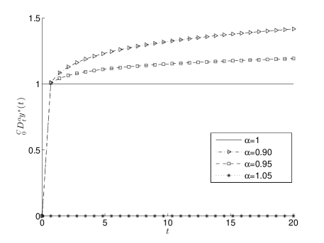
Figure 1: Derivative of $y^{*}$ and its fractional derivatives.

However, we have the following result.

Theorem 1.

Let $f:[a,b]\times\mathbb{R}\to\mathbb{R}$ be a continuous function and $\alpha>0$ a real. If $y^{*}_{\alpha}$ is a solution of the system

$$\left\{\begin{array}[]{l}{{}_{a}^{C}D_{t}^{\alpha}}y(t)=f(t,y),\quad\alpha\in(0,1)\\ y(a)=y_{a},\end{array}\right.$$

and if the limit

$$\lim_{\alpha\to 1^{\pm}}y^{*}_{\alpha}(t):=y^{*}(t)$$

exists for all $t\in[a,b]$, then $y^{*}$ is solution of the Cauchy problem

$$\left\{\begin{array}[]{l}y^{\prime}(t)=f(t,y)\\ y(a)=y_{a}.\end{array}\right.$$

Proof.

Starting with equation ${{}_{a}^{C}D_{t}^{\alpha}}y^{*}_{\alpha}(t)=f(t,y^{*}_{\alpha})$, applying the $I^{\alpha}$ operator to both sides and using Lemma 1, we obtain that $y^{*}_{\alpha}$ satisfies the Volterra equation

$$y^{*}_{\alpha}(t)=y_{a}+\frac{1}{\Gamma(\alpha)}\int_{a}^{t}(t-s)^{\alpha-1}f(s,y^{*}_{\alpha}(s))\,ds.$$

Taking the limit $\alpha\to 1^{\pm}$, we get

$$y^{*}(t)=y_{a}+\int_{a}^{t}f(s,y^{*}(s))\,ds,$$

that is, $y^{*}$ satisfies the Cauchy problem. ∎

Remark 1.

The idea of Theorem 1 is the following. We first consider a fractional differential equation of order $\alpha\in(0,1)$, and as $\alpha\to 1^{-}$, the fractional system converts into an ordinary Cauchy problem. Then, in order to obtain a higher accuracy for the method, we consider the solution of the fractional system $y^{\star}$, depending on the parameter $\alpha>0$, and compute the limit $\alpha\to 1^{\pm}$.

1.2 Computational issues

The MATLAB numerical experiments to find the model parameters as well as the non-integer derivatives that fits better in the model is carried out. The numerical experiments were done in MATLAB [8] using the routine lsqcurvefit that solves nonlinear data-fitting problems in least-squares sense, that is, given data $(y_{i})_{i=1\ldots m}$, and a model $(M_{i})_{i=1\ldots m}$, the error is:

$$E=\sum_{i=1}^{m}(y_{i}-M_{i})^{2}.$$

This routine is based on an iterative method with local convergence, i.e., depending on the initial approximation to the parameters to estimate. The initial approximations were found, based on the data analysis of each model. In the computational tests the trust-region-reflective algorithm was selected. In all the studied cases, we will see that the fractional approach is more close to the data than the classical one. To test the efficiency of the model, we compare the error of the classical model $E_{classical}$ with the error given by the fractional model $E_{fractional}$:

$$\left|\frac{E_{classical}-E_{fractional}}{E_{classical}}\right|.$$

1.3 Outline

This article is organized as follows. In each section we present a real problem, described by an ordinary or system of ordinary differential equations. We then consider the same problem, but modeled by a fractional or system of fractional differential equations, and compare which of the two models are more suitable to describe the process, based on real experimental data. Given an ordinary differential equation $y^{\prime}(t)=f(t,y)$, we replace it by the fractional differential equation ${{}_{a}^{C}D_{t}^{\alpha}}y(t)=f(t,y)$, with $\alpha\in(0,1)$. When we consider the limit $\alpha\to 1^{-}$, we obtain the initial one. If we consider $\alpha\in(1,2)$ as well, and then take the limit $\alpha\to 1^{+}$, we would get $y^{\prime}(t)-y^{\prime}(0)=f(t,y)$, and this is the reason why we will neglect this case firstly. After computing the solution of the fractional differential equation, which depends on $\alpha$, we consider the function with fractional order $\alpha$ on the interval $(0,2)$ in order to increase the accuracy of the method. Three distinct problems are studied in this paper. Section 2 deals with the exponential law of growth, and we replace it by the Mittag–Leffler function, which is a generalization of the exponential function. In Section 3 we deal with an application related to Blood Alcohol Level using integer-order derivatives. In the final Section 4 we study a model of a tape counter readings at an instant time. In each case, we compute the values of the parameters that better fit with the given data, and also the error in each of both approaches.

2 World Population Growth

2.1 Standard approach

There exist several attempts to describe the World Population Growth [11]. The simplest model is the following, known as the Malthusian law of population growth, which is used to predict populations under ideal conditions. Let $N(t)$ be the number of individuals in a population at time $t$ , $B$ and $M$ the birth and mortality rates, respectively, so that the net growth rate is given by

$$N^{\prime}(t)=(B-M)N(t)=PN(t),$$ (1)

where $P:=B-M$ is the production rate. Here, we assume that $B$ and $M$ are constant, and thus $P$ is also constant. The solution of this differential equation is the function

$$N(t)=N_{0}\mbox{e}^{Pt},\quad t\geq 0,$$ (2)

where $N_{0}$ is the population at $t=0$. Because of the solution (2), this model is also known as the exponential growth model.

2.2 Fractional approach

Considered now that the World Population Growth model is ruled by the fractional differential equation

$${{}_{0}^{C}D_{t}^{\alpha}}N(t)=PN(t),\quad t\geq 0,\,\alpha\in(0,1).$$ (3)

Observe that, taking the limit $\alpha\to 1^{-}$, Eq (3) converts into Eq. 1, but if we consider $\alpha\in(1,2)$ and take the limit $\alpha\to 1^{+}$, we obtain $N^{\prime}(t)-N^{\prime}(0)=PN(t)$.

Using Theorem 7.2 in [2], the solution of this fractional differential equation is the function

$$N(t)=N_{0}E_{\alpha}(Pt^{\alpha}),$$ (4)

where $E_{\alpha}$ is the Mittag–Leffler function

$$E_{\alpha}(t)=\sum_{k=0}^{\infty}\frac{t^{k}}{\Gamma(\alpha k+1)},\quad\,t\in\mathbb{R}.$$

Consider now function (4), with $\alpha\in(0,2)$. Then, as $\alpha\to 1^{\pm}$, we recover the solution for the classical problem (2).

2.3 Numerical experiments

For our numerical treatment of the problem, we find several databases with the world population through the centuries. Here, we use the one provided by the United Nations [13], from year 1910 until 2010, consisting in 11 values, where the initial value is $N_{0}=1750$. For the classical approach, the production rate is

$$P\approx 1.3501\times 10^{-2}$$

and the error from the data with respect to the analytic solution (2) is given by

$$E_{classical}\approx 7.0795\times 10^{5}.$$

If we take into consideration the fractional model (4), for $\alpha\in(0,2)$ we obtain that the best values are

$$\alpha=1.393298754843208\quad\mbox{and}\quad P\approx 3.4399\times 10^{-3}$$

with error

$$E_{fractional}\approx 2.0506\times 10^{5}.$$

The gain of the efficiency in this procedures is

$$\frac{7.0795\times 10^{5}-2.0506\times 10^{5}}{7.0795\times 10^{5}}\approx 0.71.$$

The graph of Figure 2 illustrates the World Population Growth model with the data, the classical model and the fractional model.

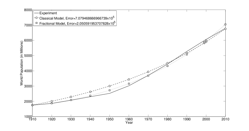
Figure 2: World Population Growth model.

3 Blood Alcohol Level problem

3.1 Standard approach

In [5] we find a simple model to determine the level of Blood Alcohol, described by a system of two differential equations. Let $A$ represent the concentration of alcohol in the stomach and $B$ the concentration of alcohol in the blood. The problem is described by the following Cauchy system:

$$\left\{\begin{array}[]{l}A^{\prime}(t)=-k_{1}A(t)\\ B^{\prime}(t)=k_{1}A(t)-k_{2}B(t)\\ A(0)=A_{0}\\ B(0)=0,\end{array}\right.$$

where $A_{0}$ is the initial alcohol ingested by the subject and $k_{1},k_{2}$ some real constants. The solution of this system is given by the two functions

$$A(t)=A_{0}\mbox{e}^{-k_{1}t}$$

and

$$B(t)=A_{0}\frac{k_{1}}{k_{2}-k_{1}}(\mbox{e}^{-k_{1}t}-\mbox{e}^{-k_{2}t}).$$

Also, in [5] some experimental data is obtained in order to determine the arbitrary constants $k_{1}$ and $k_{2}$ (Table 1). The time is in minutes and the Blood Alcohol Level (BAL) in mg/l.

Time	0	10	20	30	45	80	90	110	170
BAL	0	150	200	160	130	70	60	40	20

Table 1: Experimental data for Blood Alcohol Level.

Using the data from the table, the values that minimize the Mean Absolute Error when the values from $B$ are fitted with the experimental data are:

$$A_{0}=245.8769,\quad k_{1}=0.109456,\quad k_{2}=0.017727,$$

and the error in this approximation is

$$E_{classical}=775.2225,$$

and for comparison, and get the following results in Table 2

Time	0	10	20	30	45	80	90	110	170	Error
BAL	0	150	200	160	130	70	60	40	20	—
(Experiment)
BAL	0.0000	147.5379	172.9499	161.3813	130.0021	71.0018	59.4910	41.7418	14.4100	775.2225
(Classical)

Table 2: Experimental data vs theoretical model.

3.2 Fractional approach

Now we show that, if we consider the problem modeled by a system of fractional differential equations, we obtain a curve that better fit with the experimental results.

Let $\alpha,\beta\in(0,1)$ and consider the system of fractional differential equations

$$\left\{\begin{array}[]{l}{{}_{0}^{C}D_{t}^{\alpha}}A(t)=-k_{1}A(t)\\ {{}_{0}^{C}D_{t}^{\beta}}B(t)=k_{1}A(t)-k_{2}B(t)\\ A(0)=A_{0}\\ B(0)=0.\end{array}\right.$$

Using Theorem 7.2 in [2], the solution with respect to $A$ is

$$A(t)=A_{0}E_{\alpha}(-k_{1}t^{\alpha}).$$ (5)

To determine $B$, it can be found as the solution of the fractional differential linear equation

$${{}_{0}^{C}D_{t}^{\beta}}B(t)=-k_{2}B(t)+k_{1}A_{0}E_{\alpha}(-k_{1}t^{\alpha}).$$

By Theorem 7.2 in [2], we obtain the solution with respect to $B$:

$$\begin{array}[]{ll}B(t)&=\displaystyle\beta\int_{0}^{t}k_{1}A_{0}E_{\alpha}(-k_{1}(t-s)^{\alpha})s^{\beta-1}E^{\prime}_{\beta}(-k_{2}s^{\beta})ds\\ &=\displaystyle\beta k_{1}A_{0}\int_{0}^{t}\sum_{m=0}^{\infty}\frac{(-k_{1})^{m}(t-s)^{m\alpha}}{\Gamma(\alpha m+1)}s^{\beta-1}\sum_{n=0}^{\infty}\frac{(n+1)(-k_{2})^{n}s^{n\beta}}{\Gamma(n\beta+\beta+1)}ds\\ &\displaystyle=\beta k_{1}A_{0}\sum_{m=0}^{\infty}\sum_{n=0}^{\infty}\frac{(-k_{1})^{m}(-k_{2})^{n}(n+1)}{\Gamma(\alpha m+1)\Gamma(n\beta+\beta+1)}\int_{0}^{t}(t-s)^{m\alpha}s^{n\beta+\beta-1}ds.\end{array}$$

We remark that, as the expression inside the series is continuous and uniformly convergent, the previous calculations are valid. Let us re-write function $B(\cdot)$. Using the Beta function,

$$B(a,b)=\int_{0}^{1}t^{a-1}(1-t)^{b-1}dt,\quad a,b>0,$$

the following property

$$B(a,b)=\frac{\Gamma(a)\Gamma(b)}{\Gamma(a+b)},$$

and doing the change of variables $u=s/t$, we obtain

$$\int_{0}^{t}(t-s)^{m\alpha}s^{n\beta+\beta-1}ds=t^{m\alpha+n\beta+\beta}\int_{0}^{1}(1-u)^{m\alpha}u^{n\beta+\beta-1}du$$

$$=t^{m\alpha+n\beta+\beta}B(n\beta+\beta,m\alpha+1)=t^{m\alpha+n\beta+\beta}\frac{\Gamma(n\beta+\beta)\Gamma(m\alpha+1)}{\Gamma(n\beta+\beta+m\alpha+1)},$$

and so

$$B(t)=\displaystyle k_{1}A_{0}\sum_{m=0}^{\infty}\sum_{n=0}^{\infty}\frac{(-k_{1})^{m}(-k_{2})^{n}}{\Gamma(n\beta+\beta+m\alpha+1)}t^{m\alpha+n\beta+\beta}.$$ (6)

3.3 Numerical experiments

For computational purposes we consider the upper bounds $n=m=45$ in Eq. (6), and we intend to determine the fractional orders $\alpha$ and $\beta$ on the interval $(0,2)$, the initial value $A_{0}$, and the parameters $k_{1}$ and $k_{2}$ that best fit with the data. To that purpose, we obtain the values

$$A_{0}\approx 373.0295,\quad k_{1}\approx 0.0643,\quad k_{2}\approx 0.0088,$$

with fractional orders

$$\alpha\approx 1.1771,\quad\beta\approx 1.0052,$$

and the error in this approximation is

$$E_{fractional}\approx 321.9677.$$

By this method, the efficiency has increased

$$\frac{775.2225-321.9677}{775.2225}\approx 0.58.$$

In Table 3 we summarize the results, comparing the standard approach, using first-order derivatives, with ours using fractional-order derivatives.

Time	0	10	20	30	45	80	90	110	170	Error
BAL	0	150	200	160	130	70	60	40	20	—
(Experiment)
BAL	0.0000	147.5379	172.9499	161.3813	130.0021	71.0018	59.4910	41.7418	14.4100	775.1745
(Classical)
BAL	0.0000	155.7458	187.1950	169.6587	128.4871	69.3254	59.3669	43.7670	16.2108	321.9677
(Fractional)

Table 3: Results for the Blood Alcohol Level problem.

The graph of Figure 3 illustrates the Blood Alcohol Level with experimental data, classical model and fractional model.

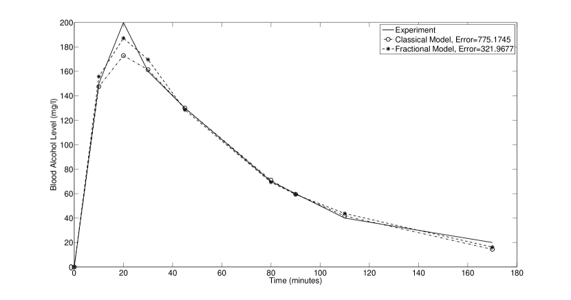
Figure 3: The blood alcohol level problem.

4 Video Tape problem

4.1 Standard approach

For the video tape problem, we intend to determine the tape counter readings $n(t)$ at an instant time $t>0$. For that, the problem is modeled in the following way. Let $c$ represents the thickness of the tape and $v$ the velocity of the tape, which is constant in time. Also, $R(t)$ indicates the radius of the wheel as is filled by the tape, and $A(t)$ measures the angle at moment $t$.

The number of revolutions is proportional to the angle, that is, $n(t)=kA(t)$, for some positive constant $k$. In [3], an ordinary differential equation is obtained to describe the behavior of the model:

$$A^{\prime}(t)=\frac{v}{R(0)\sqrt{bt+1}},\quad\mbox{where}\,b=\frac{cv}{\pi R^{2}(0)}.$$ (7)

Using the initial condition $A(0)=0$, the solution is obtained:

$$A(t)=\frac{2v}{bR(0)}(\sqrt{bt+1}-1).$$

In conclusion, the tape counter readings is given by the expression

$$n(t)=a(\sqrt{bt+1}-1),\quad\mbox{where}\,a=\frac{2kv}{bR(0)}.$$ (8)

4.2 Fractional approach

In this section we consider the video tape problem modeled by a fractional differential equation of order $\alpha\in(0,1)$:

$$\left\{\begin{array}[]{l}{{}_{0}^{C}D_{t}^{\alpha}}A(t)=\displaystyle\frac{v}{R(0)\sqrt{bt+1}},\quad\mbox{where}\,b=\frac{cv}{\pi R^{2}(0)}\\ A(0)=0\\ \end{array}\right.$$

Applying the fractional integral operator ${{}_{0}I_{t}^{\alpha}}$ to both sides of the fractional differential equation, and using Lemma 1, that reads as

$${{}_{0}I_{t}^{\alpha}}{{}_{0}^{C}D_{t}^{\alpha}}A(t)=A(t)-A(0),\quad\mbox{if}\,\alpha\in(0,1),$$

we obtain that the solution is given by

$$n(t)=\frac{p}{\Gamma(\alpha)}\int_{0}^{t}\frac{(t-s)^{\alpha-1}}{\sqrt{bs+1}}ds,\quad\mbox{where}\,p=\frac{kv}{R(0)},\,b=\frac{cv}{\pi R^{2}(0)}.$$ (9)

4.3 Numerical experiments

Using the experimental data available at http://people.uncw.edu/lugo/MCP/DIFF_EQ/deproj/deproj.htm, that counts the number of revolutions every $5$ minutes, from $t=0$ until $t=240$, we first determine the constants $a$ and $b$ for which the model given in Eq. (8) best fit the data.

$$a=988.1532\quad\mbox{and}\quad b=0.0219,$$

and the error is given by

$$E_{classical}\approx 16.7403.$$

When we consider the fractional approach, with fractional order $\alpha\in(0,2)$ for Function (9), we obtain the values

$$\alpha=0.9917,\quad p=10.9666\quad\mbox{and}\quad b=0.0199$$

with error

$$E_{fractional}\approx 16.2894.$$

For this last case, we have

$$\frac{16.7403-16.2894}{16.7403}\approx 0.03.$$

The graph of Figure 4 illustrates Video Tape model with experimental data, classical model and fractional model.

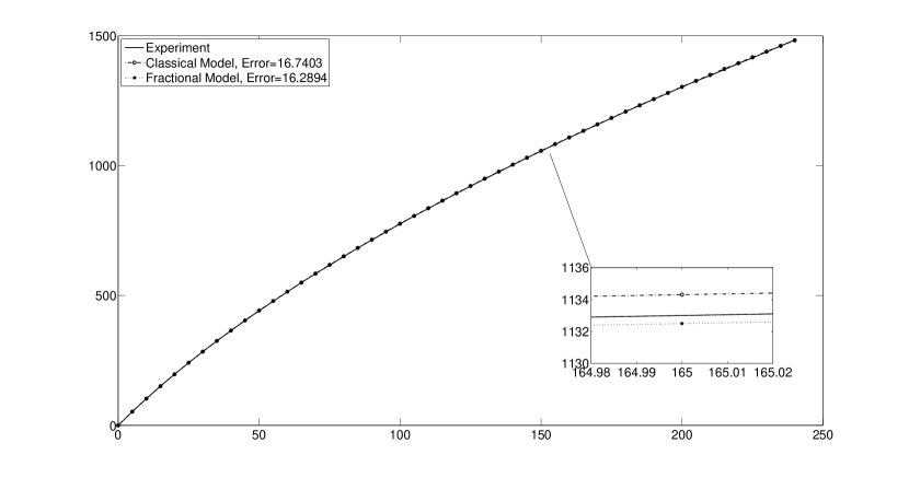
Figure 4: The Video Tape problem.

5 Conclusions

Fractional differential equations can describe better certain real world phenomena. This is understandable since systems are not usually perfect, and can be perturbed (like friction, manipulation, external forces, etc) and because of it integer-order derivatives may not be adequate to understand the trajectories of the state variables. By considering fractional derivatives, we have an infinite choices of derivative orders that we can consider, and with it determine what is the fractional differential equation that better describes the dynamics of the model. We have seen this in our experimental data, where non-integer derivatives allow the solution curve to model more efficiently the problems.

References

- [1] T.M. Atanackovic, S. Pilipovic, B. Stankovic and D. Zorica, Fractional Calculus with Applications in Mechanics: Vibrations and Diffusion Processes. Wiley-ISTE, 2014.
- [2] K. Diethelm, The Analysis of Fractional Differential Equations. An Application-Oriented Exposition Using Differential Operators of Caputo Type, LNM Springer, Volume 2004, 2010.
- [3] C. Galphin, J. Glembocki and J. Tompkins, Video Tape Counters: The Exponential Measure of Time (available online at http://people.uncw.edu/lugo/MCP/DIFF_EQ/deproj/deproj.htm)
- [4] A.A. Kilbas, H.M. Srivastava and J.J. Trujillo, Theory and Applications of Fractional Differential Equations. North-Holland Mathematics Studies, 204. Elsevier Science B.V., Amsterdam, 2006.
- [5] C. Ludwin, Blood Alcohol Content, Undergrad. J. Math. Model.: One Two 3 (2) Article 1 (2011).
- [6] J.A.T. Machado, M.F. Silva, R.S. Barbosa, I.S. Jesus, C.M. Reis, M.G. Marcos and A.F. Galhano. Some Applications of Fractional Calculus in Engineering, Mathematical Problems in Engineering, vol. 2010, Article ID 639801, 34 pages, 2010.
- [7] F.C. Meral, T.J. Royston and R. Magin, Fractional calculus in viscoelasticity: An experimental study, Commun. Nonlinear Sci. Numer. Simul. 15 (4), 939 –945 (2010).
- [8] C. Moler, J. Little, and S. Bangert, Matlab User’s Guide - The Language of Technical Computing, The MathWorks, Sherborn, Mass. (2001).
- [9] I. Podlubny, Fractional differential equations, Mathematics in Science and Engineering, 198. Academic Press, Inc., San Diego, CA, 1999.
- [10] S.G. Samko, A.A. Kilbas and O.I. Marichev, Fractional integrals and derivatives, translated from the 1987 Russian original, Gordon and Breach, Yverdon, 1993.
- [11] D.A. Smith, Human population growth: Stability or explosion? Math Mag 50 (4), 186–197 (1977).
- [12] V.E. Tarasov, Applications of Fractional Calculus to Dynamics of Particles, Fields and Media, Nonlinear Physical Science, Springer, 2010.
- [13] United Nations, The World at Six Billion Off Site, Table 1, World Population From Year 0 to Stabilization, 5, 1999.