Longitudinal spin-relaxation in nitrogen-vacancy centers in electron irradiated diamond

Abstract

We present systematic measurements of longitudinal relaxation rates ($1/T_{1}$) of spin polarization in the ground state of the nitrogen-vacancy (NV^-) color center in synthetic diamond as a function of NV^- concentration and magnetic field $B$. NV^- centers were created by irradiating a Type 1b single-crystal diamond along the [100] axis with $200\text{\,}\mathrm{keV}$ electrons from a transmission electron microscope with varying doses to achieve spots of different NV^- center concentrations. Values of ($1/T_{1}$) were measured for each spot as a function of $B$.

Nitrogen-vacancy (NV^-) centers in diamond Jelezko and Wrachtrup (2006) are useful for quantum information Gurudev Dutt et al. (2007), magnetometry (see the review by Rondin et al. Rondin et al. (2014)) and nanoscale sensing applications (see the review by Schirhagl et al. Schirhagl et al. (2014)). NV^- centers have been used to detect single electron spins Grotz et al. (2011); Mamin, Sherwood, and Rugar (2012); Shi et al. (2006) and small ensembles Mamin et al. (2013); Staudacher et al. (2013); Rugar et al. (2014); Häberle et al. (2015); DeVience et al. (2015) and single nuclear spins Sushkov et al. (2014), study magnetic resonance on a molecular scale, measure electric fields, strain and temperature, detect low concentrations of paramagnetic molecules and ions, and image magnetic field distributions of physical or biological systems. These applications are made possible by the unique properties of the NV^- center level structure, shown in Fig. 1, which allows manipulation of the ground-state spin state by optical fields and microwaves and measurement of the interactions of the ground-state spin with the local environment by monitoring the fluorescence intensity. Understanding spin relaxation processes is important in optimizing these techniques. Previous measurements of the dependence of longitudinal relaxation rate ($1/T_{1}$) of magnetic field have shown enhanced rates near $B=0$ G, $B=595$ G (Refs. Armstrong et al. (2010); Jarmola et al. (2012); V. .G. Vins et al. (2015); Mrózek et al. (2015)), and $B=514$ G (Refs.( Jarmola et al. (2012); P. Kehayias et al. (2015)). The enhancements at zero field and $B=595$ G have been linked to interactions with NV centers whose orientation makes their energies degenerate at these fields, while the enhancement at $B=514$ G is related to interactions with substitutional nitrogen (P1 centers). Previous work has also shown that the $1/T_{1}$ rate depends on NV concentration Mrózek et al. (2015). In this paper we describe systematic measurements of the longitudinal relaxation rates of ensembles of NV^- centers created with different, controlled radiation doses on a single diamond crystal, achieved through irradiation with a transmission electron microscope (TEM). This method of preparing NV^- centers is more convenient for many laboratories than irradiation in accelerators and also could facilitate the creation of microscopic structures on a diamond chip for special applications.

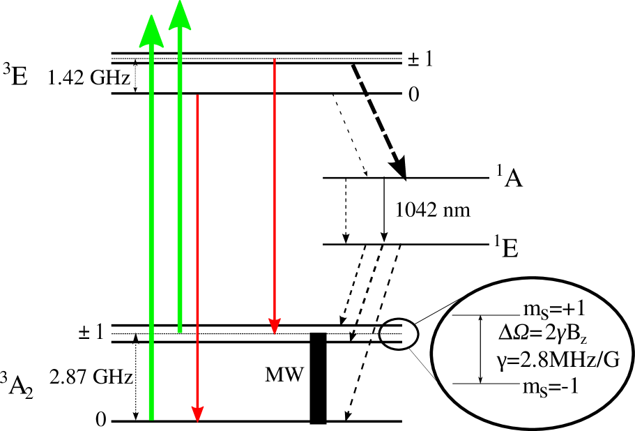
Figure 1: Energy level diagram of NV^- center. Solid vertical lines denote radiative transitions, whereas dashed lines denote transitions thought to be nonradiative.

The diamond sample was a [100] cut Type 1b single-crystal plate (Element 6), grown by the high-pressure, high-temperature technique, with an initial nitrogen concentration of 200 ppm and dimension of $3\text{\,}\mathrm{mm}$ $\times$ $3\text{\,}\mathrm{mm}$ $\times$ $0.3\text{\,}\mathrm{mm}$. It was irradiated using a transmission electron microscope Kim et al. (2012) (Tecnai G20 FEI with a Schottky field emitter electron source). The accelerating voltage was $200\text{\,}\mathrm{kV}$. At these energies the electrons can be expected to penetrate about $140\text{\,}\mathrm{\SIUnitSymbolMicro m}$ into the diamondest . However, it is unlikely that they will have sufficient energy to create vacancies below a depth of about  $20\text{\,}\mathrm{\SIUnitSymbolMicro m}$Koike, Parkin, and Mitchell (1992). Seventeen circular spots with a diameter of $10\text{\,}\mathrm{\SIUnitSymbolMicro m}$ were irradiated. After irradiation, the sample was maintained at $800\text{\,}\mathrm{\SIUnitSymbolCelsius}$ for three hours in the presence of nitrogen gas at less than atmospheric pressure. Then the sample was placed in a fluorescence microscope and illuminated with a mercury lamp through a filter cube (Olympus U-MWG2), which reflected excitation light from $510\text{\,}\mathrm{nm}$ to $550\text{\,}\mathrm{n}\mathrm{m}$ to the sample, and passed the emission through a  $590\text{\,}\mathrm{nm}$ long-pass filter. The red fluorescence was photographed with a Peltier-cooled CCD camera (GT Vision GXCAM-5C). The pixel intensities of the fluorescence are shown in Fig. 2; the irradiation parameters of the samples are given in Table 1. Spots 5–13 were irradiated with an electron intensity of $3530\text{\,}{\mathrm{nm}}^{-2}\text{\,}{\mathrm{s}}^{-1}$ to reach the dose listed in the table. Spot 14 was obtained by irradiating with an electron intensity of $2530\text{\,}{\mathrm{nm}}^{-2}\text{\,}{\mathrm{s}}^{-1}$ to compare results for irradiation at different rates but same total intensity.

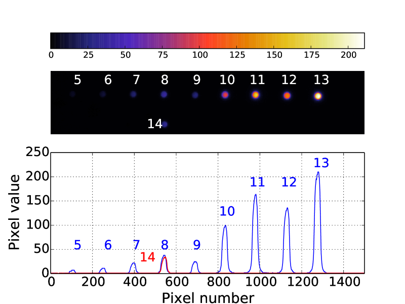
Figure 2: Fluorescence microscope image of the irradiated and annealed sample with a cross-section of fluorescence intensity. The colorbar indicates the intensity of the fluorescence.

Table 1: Parameters of the irradiated spots numbered as per the labels in Fig. 2: Integrated (red) fluorescence intensity upon irradiation with green light, electron dose and estimated NV^- concentration.

	Integrated	Electron	Estimated
	Fluorescence	Dose	NV-
Spot	Intensity		Concentration
Nr.	(arb. units)	(${\mathrm{cm}}^{-2}$)	(ppm)
5	1400	$1.1\times 10^{19}$	0.2
6	2600	$2.1\times 10^{19}$	0.3
7	5700	$4.2\times 10^{19}$	0.7
8	10000	$8.5\times 10^{19}$	1.2
9	6300	$1.7\times 10^{20}$	0.7
10	2900	$3.4\times 10^{20}$	3.3
11	50000	$6.8\times 10^{20}$	5.5
12	39000	$1.3\times 10^{21}$	4.3
13	65000	$2.5\times 10^{21}$	7.1
14	8300	$6.1\times 10^{19}$	3.9

The experimental setup used to measure longitudinal relaxation times as a function of magnetic field is shown in Fig. 3. One should note that our procedure assumes that the relaxation rates for the $m_{S}=0$ and $m_{S}=\pm 1$ sublevels are identical. NV centers were excited with $512\text{\,}\mathrm{nm}$ light from an external cavity diode laser (Toptica DL100 pro). The laser power before the microscope lens was around $7\text{\,}\mathrm{mW}$. The microscope lens had a focal length of  $4.5\text{\,}\mathrm{mm}$ and numerical aperture of 0.55. The sample holder was mounted on a three-axis positioning stage (Thorlabs Max341) and placed inside a three-axis Helmholtz coil system, allowing control over the magnetic field direction and magnitude. Microwaves (MW) from a frequency generator (Stanford Research Systems SG386) passed through a switch (Minicircuits ZASWA-2-50DR+) and were amplified with a $16\text{\,}\mathrm{W}$ MW amplifier (Minicircuits ZHL-16W-43-S+). The MW were delivered to the sample by a $0.071\text{\,}\mathrm{mm}$ diameter copper wire placed close to the diamond surface, and the wire was terminated into $50\text{\,}\mathrm{o}\mathrm{h}\mathrm{m}$ after the sample.

The fluorescence from the sample was collected using the same microscope lens that focused the light onto the sample, and then passed through a dichroic mirror (Thorlabs DMLP567), which passed wavelengths longer than $567\text{\,}\mathrm{nm}$. After passing through an additional filter that further suppressed the green excitation light, the fluorescence could be deflected to either a CMOS camera for visual adjustments of the sample, wire or position on sample, or to the avalanche photodiode (Thorlabs APD110A/M) for overall fluorescence measurements.

The current in the Helmholtz coils was adjusted so that the magnetic field pointed in the [111] crystallographic direction. An optically detected magnetic resonance (ODMR) signal was obtained by scanning the microwave frequency under continuous laser irradiation and measuring the fluorescence (see Fig. 4). In this configuration two ODMR peaks appear on either side of the microwave frequency of $2.87\text{\,}\mathrm{GHz}$, which is the frequency of the NV resonance in the absence of magnetic field. The two inner peaks are more intense and correspond to the three possible alignments of the NV axis that make the same angle with the magnetic field. The two outer peaks correspond to the alignment of the NV axis that is parallel to the magnetic field. Then, the microwave generator was set to the frequency corresponding to one of the outer ODMR peaks (both were measured).

The laser light hitting the sample could be turned on and off with an accousto-optic modulator (AA OptoElectronic MT200-A0.5-VIS). An pulse generator (PulseBlaster ESR-PRO-500) was used to control the accousto-optic modulator and MW switch. To measure the longitudinal relaxation time, a decay curve was generated as follows. First, the NV^- centers were pumped into $m_{S}=0$ level of the ground state with a green laser pulse that lasted $50\text{\,}\mathrm{\SIUnitSymbolMicro s}$. Then the laser light was blocked for a variable time $\tau$, after which the sample was again illuminated. The fluorescence as a function of time was recorded on an oscilloscope (Yokogawa DL6154), averaged 1024 times and saved to disk. The procedure was repeated, but a microwave $\pi$ pulse was applied after the laser pump pulse. This sequence was repeated five times. The fluorescence obtained after time $\tau$ with the $\pi$ pulse was subtracted from the fluorescence obtained after time $\tau$ without the $\pi$ pulse to eliminate contributions to the signal from other NV^- alignments and other sources of common-mode noise Jarmola et al. (2012). The fluorescence immediately after time $\tau$ was normalized to the fluorescence after the spins have been pumped into the $m_{S}=0$ ground-state sublevel, and this quantity $I$ was plotted as a function of $\tau$. The plot was fit with a stretched exponential of the form $\exp{-(\frac{\tau}{T_{1}})^{\beta}}$, where $T_{1}$ is the longitudinal relaxation time, and $\beta$ is a parameter between zero and one that describes the distribution of relaxation times in a large ensemble of NV^- centers with similar but not identical relaxation times. A value of $\beta=1$ indicates a $\delta$-function distribution of relaxation times Johnston (2006).

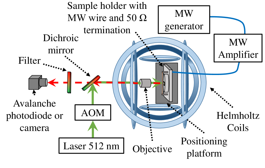
Figure 3: Schematic diagram of the experiment.

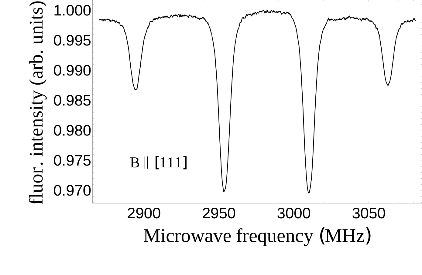
Figure 4: Fluorescence vs. MW frequency at $B=30$ G.

In order to compare the NV concentrations of the different spots, we measured their fluorescence with a fluorescence microscope (see Fig. 2). The relationship between the fluorescence intensity and NV^- concentration was determined using a diamond sample with a known, uniform NV^- concentration of 10 ppm in the same setup. Assuming that the fluorescence intensity is proportional to the NV^- concentration, the relative concentration of our spots should be relatively well known (see Fig. 5). However, the overall normalization should be considered to be only an order-of-magnitude estimate. Our estimated NV^- concentrations are systematically lower than concentrations quoted for similar electron doses Acosta et al. (2010); Jarmola et al. (2012); Mrózek et al. (2015); however, these experiments used higher electron energies.

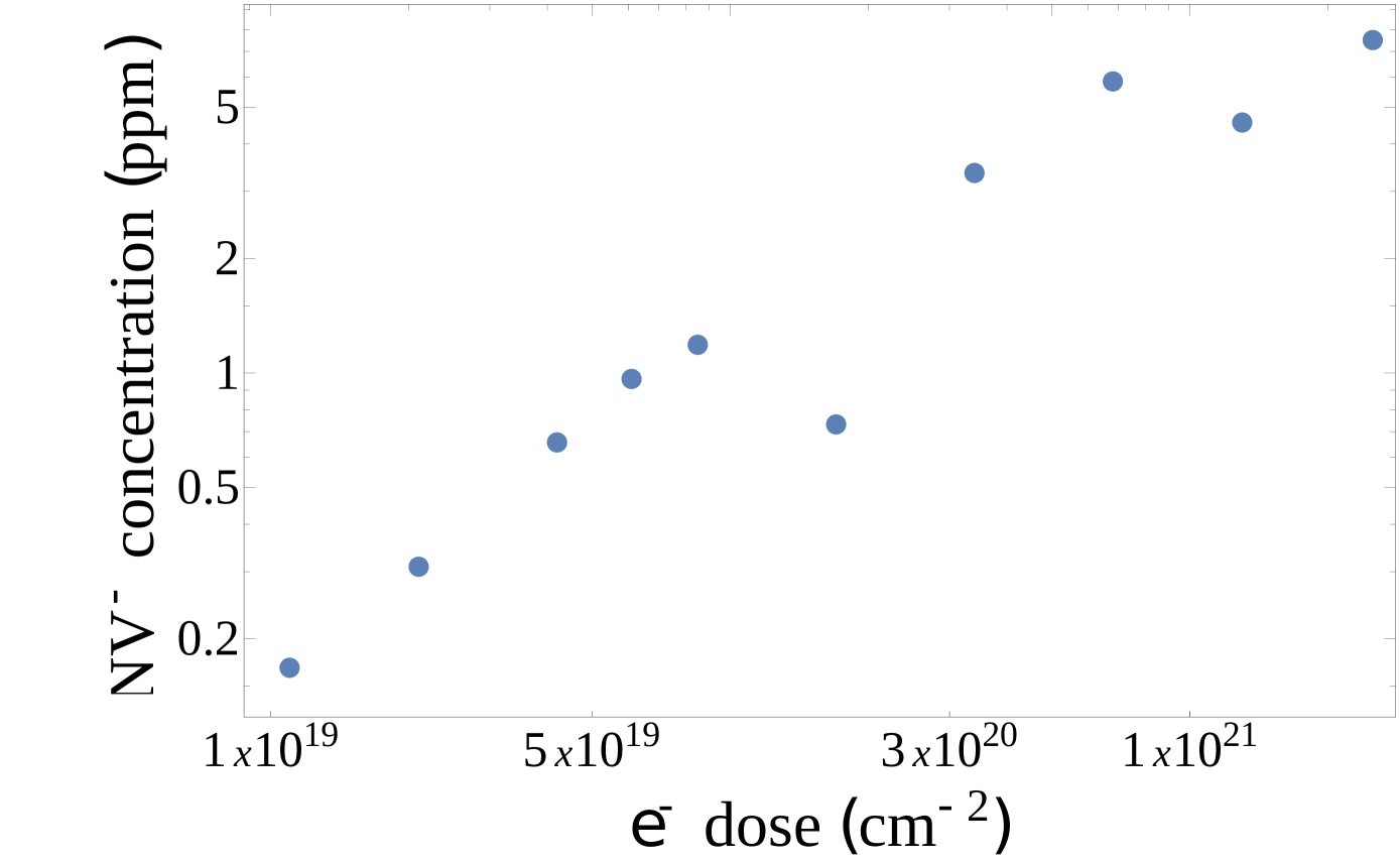
Figure 5: Estimated NV^- concentration vs electron dose. Error bars are not given as the main error is systematic and could be a factor of five.

The Hamiltonian $H_{S}$ of the ${}^{3}A_{2}$ state (see Fig. 1) of the electronic spin of the NV^- center is given by $H_{S}=DS_{z}^{2}+E(S_{x}^{2}-S_{y}^{2})+g_{S}\mu_{B}\vec{B}\cdot\vec{S}$, where $DS_{z}^{2}$ corresponds to the zero-field splitting, $E(S_{x}^{2}-S_{y}^{2})$ corresponds to electric fields, which can arise in the lattice due to strain, and $g_{S}\mu_{B}\vec{B}\cdot\vec{S}$ corresponds to the Zeeman splitting. The strain parameter $2E$ can be observed as a small splitting in the zero-field ODMR signal. We have estimated this parameter for each spot by fitting parabolas to the peaks, and it is plotted in Fig. 6 as a function of estimated concentration. The radiation damage causes distortions in the crystal structure, as shown by the fact that the strain splitting increases with concentration, though more slowly above $~{}3$ ppm. The distortion could also change the distance between the N and V defects, which would alter the zero-field splitting $D$. Whereas an earlier study reported an increase of the zero-field splitting $D$ on the order of 20 MHz at high radiation doses Kim et al. (2012), our measurements show no change in $D$.

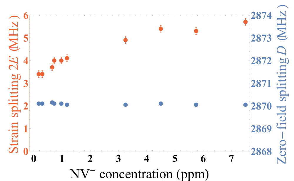
Figure 6: Strain splitting ($2E$) and zero-field splitting ($D$) as a function of NV^- concentration.

Figure 7 shows the measured longitudinal relaxation rates, obtained by fitting the decay curves from our experiments, as a function of magnetic field for various spots. The rates are comparable to previously measured rates in bulk samples Jarmola et al. (2012); Mrózek et al. (2015). The increase in $1/T_{1}$ at zero magnetic field is caused by the fact that all ODMR components are degenerate thereMrózek et al. (2015). The effect is analogous to level-crossing resonances. It is also possible to see a hint of the relaxation rates dropping and increasing again as the magnetic field value increases from zero, which is related to partial overlapping of the ODMR components at lower magnetic field valuesMrózek et al. (2015). More measurements near zero field would be desirable, but we could not resolve the $\pm 1$ ODMR peaks at lower fields.

Figure 8 shows that in our fits the value of $\beta$ approaches unity as the NV^- concentration decreases. This result is consistent with the measurements in Fig. 2(a) of Jarmola et al. (2012), which showed that at low temperatures, the NV^- density, i.e., interaction with nearby spins, dominated the $1/T_{1}$ rate, wherease at higher temperatures, relaxation induced by phonons dominated. Similarly, the nearly linear relationship between longitudinal relaxation rate and NV concentration is consistent with dipole-dipole interactions driving relaxation at these densities, since the dipole field drops off as $r^{-3}$ whereas the average distance to the nearest NV center changes as $\rho^{-1/3}$.

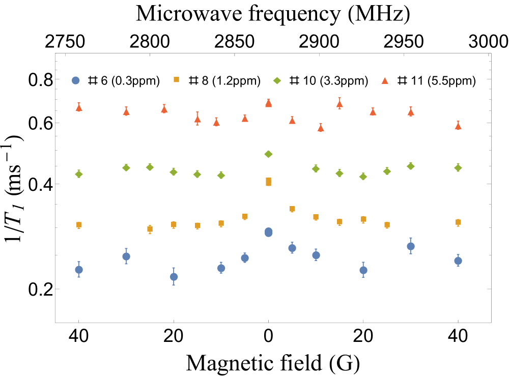
Figure 7: Longitudinal relaxation rates as a function of magnetic field for different spots.

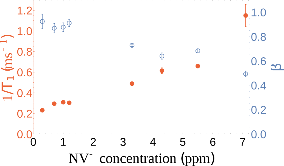
Figure 8: $1/T_{1}$ (filled circles) and the parameter $\beta$ (open circles) as a function NV^- concentration at $B=30$ G.

In conclusion, we have made a systematic measurement of longitudinal relaxation times as a function of magnetic field and and NV^- concentration for a type Ib diamond. The results suggest that at high concentrations the NV^- centers in the spots do not have a narrowly defined relaxation rate, but rather some distribution of relaxation rates. However, as the concentration decreases, the relaxation rate becomes better defined, as indicated by the stretched-exponential fits of the polarization-decay curves approaching unity. Another interesting feature is the zero-field resonance in relaxation rate when plotted against magnetic field (Fig. 7) Jarmola et al. (2012); Mrózek et al. (2015). Finally, the longitudinal relaxation rate was measured for values of NV^- concentration spanning an order of magnitude, and the value of the relaxation rate increased by almost a factor of five over this range. These measurements could help to guide the preparation of microscale NV^- sensors on diamond using a TEM.

This work was supported by ESF Project Nr. 2013/0028/1DP/1.1.1.2.0/13/APIA/VIAA/054. We thank Raimonds Poplausks and Kaspars Vaičekonis for help with the experiments. D.B. acknowledges support by DFG through the DIP program (FO 703/2-1) and by the AFOSR/DARPA QuASAR program.

References

- Jelezko and Wrachtrup (2006) F. Jelezko and J. Wrachtrup, phys. stat. sol.(a) 203, 3207 (2006).
- Gurudev Dutt et al. (2007) M. V. Gurudev Dutt, L. Childress, L. Jiang, E. Togan, J. Maze, F. Jelezko, A. S. Zibrov, P. R. Hemmer, and M. D. Lukin, Science 316, 1312 (2007).
- Rondin et al. (2014) L. Rondin, J.-P. Tetienne, T. Hingant, J.-F. Roch, P. Maletinsky, and V. Jacques, Reports on Progress in Physics 77, 056503 (2014).
- Schirhagl et al. (2014) R. Schirhagl, K. Chang, M. Loretz, and C. L. Degen, Annual Review of Physical Chemistry 65, 85 (2014).
- Grotz et al. (2011) B. Grotz, J. Beck, P. Neumann, B. Naydenov, R. Reuter, F. Reinhard, F. Jelezko, J. Wrachtrup, D. Schweinfurth, B. Sarkar, and P. Hemmer, New. J. Phys. 13, 055004 (2011).
- Mamin, Sherwood, and Rugar (2012) H. J. Mamin, M. H. Sherwood, and D. Rugar, Phys. Rev. B 86, 195422 (2012).
- Shi et al. (2006) F. Shi, Q. Zhang, P. Wang, H. Sun, J. Wang, X. Rong, M. Chen, C. Ju, F. Reinhard, H. Chen, J. Wrachtrup, J. Wang, and J. Du, Science 347, 1135 (2006).
- Mamin et al. (2013) H. J. Mamin, M. Kim, M. H. Sherwood, C. T. Rettner, K. Ohno, D. D. Awschalom, and D. Rugar, Science 339, 557 (2013).
- Staudacher et al. (2013) T. Staudacher, F. Shi, S. Pezzagna, J. Meijer, J. Du, C. A. Meriles, F. Reinhard, and J. Wrachtrup, Science 339, 561 (2013).
- Rugar et al. (2014) D. Rugar, H. J. Mamin, M. H. Sherwood, M. Kim, C. T. Rettner, K. Ohno, and D. D. Awschalom, Nature Nanotechnology 10, 120 (2014).
- Häberle et al. (2015) T. Häberle, D. Schmid-Lorch, R. Reinhard, and J. Wrachtrup, Nature Nanotechnology 10, 125 (2015).
- DeVience et al. (2015) S. J. DeVience, L. M. Pham, I. Lovchinsky, A. O. Sushkov, N. Bar-Gill, C. Belthangady, F. Casola, M. Corbett, H. Zhang, M. Lukin, H. Park, A. Yacoby, and R. L. Walsworth, Nature Nanotechnology 10, 129 (2015).
- Sushkov et al. (2014) A. O. Sushkov, I. Lovchinsky, N. Chisholm, R. L. Walsworth, H. Parki, and M. D. Lukin, Phys. Rev. Lett. 113, 197601 (2014).
- Armstrong et al. (2010) S. Armstrong, L. J. Rogers, R. L. McMurtrie, and N. B. Manson, Physics Procedia 3, 1569 (2010).
- Jarmola et al. (2012) A. Jarmola, V. M. Acosta, K. Jensen, S. Chemerisov, and D. Budker, Phys. Rev. Lett. 108, 197601 (2012).
- V. .G. Vins et al. (2015) S. V. A. V. .G. Vins, A. P. Yelisseyev, N. N. Lukzen, N. L. Lavrik, and V. A. Bagryansky, New J. Phys. 17, 023040 (2015).
- Mrózek et al. (2015) M. Mrózek, D. Rudnicki, P. Kehayias, A. Jarmola, D. Budker, and W. Gawlik, EPJ Quantum Technology 2, 22 (2015), arXiv:1505.02253 .
- P. Kehayias et al. (2015) L. T. H. P. Kehayias, D. A. Simpson, A. Jarmola, A. Stacey, D. Budker, and L. C. L. Hollenberg, arXiv 1503.00830v1 (2015).
- Kim et al. (2012) E. Kim, V. M. Acosta, E. Bauch, D. Budker, and P. R. Hemmer, Applied Physics Letters 101, 082410 (2012).
- (20) “ESTAR Database,” http://physics.nist.gov/PhysRefData/Star/Text/ESTAR.html, accessed: 2015-29-08.
- Koike, Parkin, and Mitchell (1992) J. Koike, D. M. Parkin, and T. E. Mitchell, Applied Physics Letters 60, 1450 (1992).
- Johnston (2006) D. C. Johnston, Phys. Rev. B 74, 184430 (2006).
- Acosta et al. (2010) V. M. Acosta, E. Bauch, M. P. Ledbetter, A. Waxman, L.-S. Bouchard, and D. Budker, Phys. Rev. Lett. 104, 070801 (2010).