What Players do with the Ball: A Physically Constrained Interaction Modeling

Abstract

Tracking the ball is critical for video-based analysis of team sports. However, it is difficult, especially in low-resolution images, due to the small size of the ball, its speed that creates motion blur, and its often being occluded by players.

In this paper, we propose a generic and principled approach to modeling the interaction between the ball and the players while also imposing appropriate physical constraints on the ball’s trajectory.

We show that our approach, formulated in terms of a Mixed Integer Program, is more robust and more accurate than several state-of-the-art approaches on real-life volleyball, basketball, and soccer sequences.

1 Introduction

Tracking the ball accurately is critically important to analyze and understand the action in sports ranging from tennis to soccer, basketball, volleyball, to name but a few. While commercial video-based systems exist for the first, automation remains elusive for the others. This is largely attributable to the interaction between the ball and the players, which often results in the ball being either hard to detect because someone is handling it or even completely hidden from view. Furthermore, since the players often kick it or throw it in ways designed to surprise their opponents, its trajectory is largely unpredictable.

There is a substantial body of literature about dealing with these issues, but almost always using heuristics that are specific to a particular sport such as soccer [31], volleyball [10], or basketball [6]. A few more generic approaches explicitly account for the interaction between the players and the ball [28] while others impose physics-based constraints on ball motion [23]. However, neither of these things alone suffices in difficult cases, such as the one depicted by Fig. 1.

In this paper, we, therefore, introduce an approach to simultaneously accounting for ball/player interactions and imposing appropriate physics-based constraints. Our approach is generic and applicable to many team sports. It involves formulating the ball tracking problem in terms of a Mixed Integer Program (MIP) in which we account for the motion of both the players and the ball as well as the fact the ball moves differently and has different visibility properties in flight, in possession of a player, or while rolling on the ground. We model the ball locations in $\mathbb{R}^{3}$ and impose first and second-order constraints where appropriate. The resulting MIP describes the ball behaviour better than previous approaches [28, 23] and yields superior performance, both in terms of tracking accuracy and robustness to occlusions. Fig. 1(c) depicts the improvement resulting from doing this rather than only modeling the interactions or only imposing the physics-based constraints.

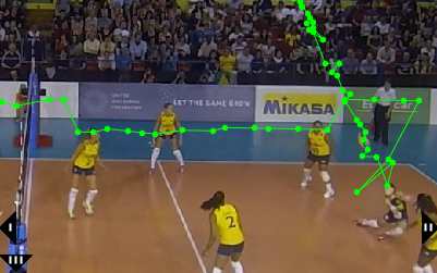
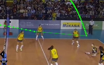
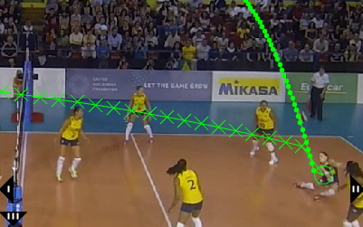
(a)	(b)	(c)

Figure 1: Importance of simultaneously modeling interactions and imposing physical constraints. For most of this 70-frame volleyball sequence depicting the ball crossing the net and being bumped by a defending player and viewed by 3 cameras, the defending player is on the ground. As a result, she was not detected by the person detector we use [9] because it only finds people standing up. Furthermore, while the ball was near the player, it was occluded in the views of 2 of the 3 cameras, and, therefore, not detected as a 3D object. (a) Tracking the players and the ball simultaneously without imposing motion constraints as in [28] produces physically impossible trajectories. (b) Imposing motion constraints but tracking the players and the ball separately as in [23] does not properly capture the ball and player interaction. (c) Our approach to both imposing constraints and modeling the interaction gives a better overall result. The crosses denote the fact that the ball is in the “strike” state until being bumped and in the “flying” one after that. Transitions between these states can only result from interacting with a player, which encourages the optimizer to find one in spite of the weak evidence. Best viewed in color.

In short, our contribution is a principled and generic formulation of the ball tracking problem and related physical constraints in terms of a MIP. We will demonstrate that it outperforms state-of-the-art approaches [27, 28, 23, 10] in soccer, volleyball, and basketball.

2 Related work

While there are approaches to game understanding, such as [16, 19, 20, 11, 7, 15], which rely on the structured nature of the data without any explicit reference to the location of the ball, most others either take advantages of knowing the ball position or would benefit from being able to [7]. However, while the problem of automated ball tracking can be considered as solved for some sports such as tennis or golf, it remains difficult for team sports. This is particularly true when the image resolution is too low to reliably detect the ball in individual frames in spite of frequent occlusions.

Current approaches to detecting and tracking can be roughly classified as those that build physically plausible trajectory segments on the basis of sets of consecutive detections and those that find a more global trajectory by minimizing an objective function. We briefly review both kinds below.

2.1 Fitting Tracjectory Segments

Many ball-tracking approaches for soccer [21, 18], basketball [6], and volleyball [5, 10, 4] start with a set of successive detections that obey a physical model. They then greedily extend them and terminate growth based on various heuristics. In [25], Canny-like hysteresis is used to select candidates above a certain confidence level and link them to already hypothesized trajectories. Very recently, RANSAC has been used to segment ballistic trajectories of basketball shots towards the basket [23]. These approaches often rely heavily on domain knowledge, such as audio cues to detect ball hits [5] or model parameters adapted to specific sports [4, 6].

While effective when the initial ball detections are sufficiently reliable, these methods tend to suffer from their greedy nature when the quality of these detections decreases. We will show this by comparing our results to those of [10, 23], for which the code is publicly available and have been shown to be a good representatives of this set of methods.

2.2 Global Energy Minimization

One way to increase robustness is to seek the ball trajectory as the minimum of a global objective function. It often includes high-level semantic knowledge such as players’ locations [32, 31, 27], state of the game based on ball location, velocity and acceleration [31, 32], or goal events [32].

In [28, 29], the players and the ball are tracked simultaneously and ball possession is explicitly modeled. However, the tracking is performed on a discretized grid and without physics-based constraints, which results in reduced accuracy. It has nevertheless been shown to work well on soccer and basketball data. We selected it as our baseline to represent this class of methods, because of its state-of-the-art results and publicly available implementation.

3 Problem Formulation

We consider scenarios where there are several calibrated cameras with overlapping fields of view capturing a substantial portion of the play area, which means that the apparent size of the ball is generally small. In this setting, trajectory growing methods do not yield very good results both because the ball is occluded too often by the players to be detected reliably and because its being kicked or thrown by them result in abrupt and unpredictable trajectory changes.

To remedy this, we explicitly model the interaction between the ball and the players as well as the physical constraints the ball obeys when far away from the players. To this end, we first formulate the ball tracking problem in terms of a maximization of a posteriori probability. We then reformulate it in terms of an integer program. Finally, by adding various constraints, we obtain the final problem formulation that is a Mixed Integer Program.

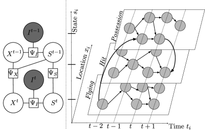
(a)                             (b)

Figure 2: Graphical models. (a) Factor graph for ball tracking. At each time instant $t$, we consider the ball location $X^{t}$ and state $S^{t}$ along with the available image evidence $I^{t}$. (b) Ball graph used to formulate the integer program. To each node $i$, is associated a location $x_{i}$, a state $s_{i}$, and a time instant $t_{i}$. The relationship between the variables in both graphs is spelled out in Eqs 3(d,e).

$T,K$	Number of temporal frames and ball states
$I^{t}$	Image evidence at time $t$
$X^{t},S^{t}$	Discrete location and state of the ball at time $t$
$P^{t}$	3D coordinates of the ball at time $t$
$i,j,k,l$	Node indices in the ball or players graph
$V_{b},V_{p}$	Sets of nodes in ball and player graphs
$E_{b},E_{p}$	Sets of edges in the ball and player graphs
$x_{i},s_{i},t_{i}$	Discrete location, state, and time of node $i$
$S_{b}$	Special node for the ball at $t=0$
$S_{p},T_{p}$	Source and sink nodes of player trajectories
$f_{i}^{j},p_{i}^{j}$	Number of balls and players moving from $i$ to $j$
$c_{bi}^{j}$,$c_{pi}^{j}$	Ball and player transition costs from $i$ to $j$
$\Psi_{X},\Psi_{S},\Psi_{I}$	Position, state, image evidence potentials
$\psi$	Potential of local image evidence
$D_{l}$	Max. permissible distance between $X^{t}$ and $P^{t}$
$D_{p}$	Max. permissible distance for ball possession
$A^{s,c},B^{s,c}$	Physics-based constants for state $s$, axis $c$
$C^{s,c},F^{c,s}$
$O^{s,c}$	Constraint-free locations for state $s$ and axis $c$
$\mathbb{F}$	Permissible ball locations and state sequences

Table 1: Notations

3.1 Graphical Model for Ball Tracking

We model the ball tracking process from one frame to the next in terms of the factor graph depicted by Fig. 2(a). We associate to each instant $t\in\left\{1\ldots T\right\}$ three variables $X^{t}$, $S^{t}$, and $I^{t}$, which respectively represent the 3D ball position, the state of the ball, and the available image evidence. When the ball is within the capture volume, $X^{t}$ is a 3D vector and $S^{t}$ can take values such as flying or in_possession, which are common to all sports, as well as sport-dependent ones, such as strike for volleyball or pass for basketball. When the ball is not present, we take $X^{t}$ and $S^{t}$ to be $\infty$ and not_present respectively. These notations as well as all the others we use in this paper are summarized in Table 1.

Given the conditional independence assumptions implied by the structure of the factor graph of Fig. 2(a), we can formulate our tracking problem as one of maximizing the energy function

$$\Psi(X,S,I) = {1\over Z}\Psi_{I}(X^{1},S^{1},I^{1})\prod\limits_{t=2}^{T}\Big{[}\Psi_{X}(X^{t-1},S^{t-1},X^{t})$$ (1)

$$\Psi_{S}(S^{t-1},S^{t})\Psi_{I}(X^{t},S^{t},I^{t})\Big{]}$$

expressed in terms of products of the following potential functions:

• $\Psi_{I}(X^{t},S^{t},I^{t})$ encodes the correlation between the ball position, ball state, and the image evidence.

• $\Psi_{S}(S^{t-1},S^{t})$ models the temporal smoothness of states across adjacent frames.

• $\Psi_{X}(X^{t-1},S^{t-1},X^{t})$ encodes the correlation between the state of the ball and the change of ball position from one frame to the next one.

• $\Psi_{X}(X^{1},S^{1},X^{2})$ and $\Psi_{S}(S^{1},S^{2})$ include priors on the state and position of the ball in the first frame.

In practice, as will be discussed in Sec. 4, the $\Psi$ functions are learned from training data. Let $\mathbb{F}$ be the set of all possible sequences of ball positions and states. We consider the log of Eq. 1 and drop the constant normalization factor $\log Z$. We, therefore, look for the most likely sequence of ball positions and states as

$$(X^{*},S^{*})=\arg\max\limits_{(X,S)\in\mathbb{F}}\sum\limits_{t=2}^{T}\Big{[}\log\Psi_{X}(X^{t-1},S^{t-1},S^{t})+$$ (2)

$$\log\Psi_{S}(S^{t-1},S^{t})+\log\Psi_{I}(X^{t},S^{t},I^{t})\Big{]}+\log\Psi_{I}(X^{1},S^{1},I^{1})\;.$$

In the following subsections, we first reformulate this maximization problem as an integer program and then introduce additional physics-based and in_possession constraints.

3.2 Integer Program Formulation

To convert the maximization problem of Eq. 2 into an Integer Program (IP), we introduce the ball graph $G_{b}=(V_{b},E_{b})$ depicted by Fig. 2(b). $V_{b}$ represents its nodes, whose elements each correspond to a location $x_{i}\in\mathbb{R}^{3}$, state $s_{i}\in\{1,\cdots,K\}$, and time index $t_{i}\in\{1,\cdots,T\}$. In practice, we instantiate as many as there are possible states at every time step for every actual and potentially missed ball detection. Our approach to hypothesizing such missed detections is described in Sec. 5. $V_{b}$ also contains an additional node $S_{b}$ denoting the ball location before the first frame. $E_{b}$ represents the edges of $G_{b}$ and comprises all pairs of nodes corresponding to consecutive time instants and whose locations are sufficiently close for a transition to be possible.

Let $f_{i}^{j}$ denote the number of balls moving from $i$ to $j$ and $c_{bi}^{j}$ denote the corresponding cost. The maximization problem of Eq. 2 can be rewritten as

$$\text{maximize}\displaystyle\sum\limits_{(i,j)\in E_{b}}f_{i}^{j}c_{bi}^{j}\;,$$ (3)

where
$c_{bi}^{j}=\log\Psi_{X}(x_{i},s_{i},x_{j})+\log\Psi_{S}(s_{i},s_{j})+\log\Psi_{I}(x_{j},s_{j},I^{t_{j}}),$
subject to

$$\begin{array}[]{ll@{}ll}&\textit{(a)}&\mbox{\hskip 8.53581pt}f_{i}^{j}\in\{0,1\}&\mbox{}\forall(i,j)\in E_{b}\\ &\textit{(b)}&\mbox{\hskip 8.53581pt}\sum\limits_{(i,j)\in E_{b},t_{j}=1}f_{i}^{j}=1&\\ &\textit{(c)}&\mbox{\hskip 8.53581pt}\sum\limits_{(i,j)\in E_{b}}f_{i}^{j}=\sum\limits_{(j,k)\in E_{b}}f_{j}^{k}&\mbox{}\forall j\in V_{b}:0<t_{j}<T\\ &\textit{(d)}&\mbox{\hskip 8.53581pt}X^{t}=\sum\limits_{(i,j)\in E_{b},t_{j}=t}f_{i}^{j}x_{j}&\mbox{}\forall t\in 1,\cdots,T\\ &\textit{(e)}&\mbox{\hskip 8.53581pt}S^{t}=\sum\limits_{(i,j)\in E_{b},t_{j}=t}f_{i}^{j}s_{j}&\mbox{}\forall t\in 1,\cdots,T\\ &\textit{(f)}&\mbox{\hskip 8.53581pt}(X,S)\in\mathbb{F}&\\ \end{array}$$

We optimize with respect to the $f_{i}^{j}$, which can be considered as flow variables. The constraints of Eqs.3(a-c) ensure that at every time frame there exists only one position and one state to which the only ball transitions from the previous frame. The constraint of Eq.3(f) is intended to only allow feasible combinations of locations and states as described by the set $\mathbb{F}$, which we define below.

3.3 Mixed Integer Program Formulation

Some ball states impose first and second order constraints on ball motion, such as zero acceleration for the freely flying ball or zero vertical velocity and limited negative acceleration for the rolling ball. Possession implies that the ball must be near the player.

In this section, we assume that the players’ trajectories are available in the form of a player graph $G_{p}=(V_{p},E_{p})$ similar to the ball graph of Sec. 3.2 and whose nodes comprise locations $x_{i}$ and time indices $t_{i}$. In practice, we compute it using publicly available code as described in Sec. 5.1.

Given $G_{p}$, the physics-based and possession constraints can be imposed by introducing auxiliary continuous variables and expanding constraint of Eq. 3(f), as follows.

Continuous Variables.

The $x_{i}$ represent specific 3D locations where the ball could potentially be, that is, either actual ball detections or hypothesized ones as will be discussed in Sec. 5.2. Since they cannot be expected to be totally accurate, let the continuous variables $P^{t}=(P_{x}^{t},P_{y}^{t},P_{z}^{t})$ denote the true ball position of at time $t$. We impose

$$||P^{t}-X^{t}||\leq D_{l}$$ (4)

where $D_{l}$ is a constant that depends on the expected accuracy of the $x_{i}$. These continuous variables can then be used to impose ballistic constraints when the ball is in flight or rolling on the ground as follows.

Second-Order Constraints.

For each state $s$ and coordinate $c$ of $P$, we can formulate a second-order constraint of the form

$$A^{s,c}(P^{t}_{c}-2P^{t-1}_{c}+P^{t-2}_{c})+B^{s,c}(P^{t}_{c}-P^{t-1}_{c})+$$ (5)

$$C^{s,c}P^{t}_{c}-F^{s,c}\leq K(3-M^{t}_{s,c}-M^{t-1}_{s,c}-M^{t-2}_{s,c})\;,$$

$$\mbox{where}\,\,M^{t}_{s,c}=\sum\limits_{(i,j)\in E_{b},t_{j}=t,s_{j}=s,x_{j}\not\in O^{s,c}}f_{i}^{j}\;,$$

$K$ is a large positive constant and $O^{s,c}$ denotes the locations where there are scene elements with which the ball can collide, such as those near the basketball hoops or close to the ground. Given the constraints of Eq. 3, $M^{t}_{s,c}$, $M^{t-1}_{s,c}$, and $M^{t-2}_{s,c}$ must be zero or one. This implies that right side of the above inequality is either zero if $M^{t}_{s,c}=M^{t-1}_{s,c}=M^{t-2}_{s,c}=1$ or a large number otherwise. In other words, the constraint is only effectively active in the first case, that is, when the ball consistently is in a given state. When this is the case, $(A^{s,c},B^{s,c},C^{s,c}$,$F^{s,c})$ model the corresponding physics. For example, when the ball is in the flying state, we use $(1,0,0,{-g\over fps^{2}})$ for the $z$ coordinate to model the parabolic motion of an object subject to the sole force of gravity whose intensity is $g$. In the rolling state, we use $(1,0,0,0)$ for both the $x$ and $y$ coordinates to denote a constant speed motion in the $xy$ plane. In both cases, we neglect the effect of friction. We give more details for all states we represent in the supplementary materials. Note that we turn off these constraints altogether at locations in $O^{s,c}$.

Possession constraints.

While the ball is in possession of a player, we do not impose any physics-based constraints. Instead, we require the presence of someone nearby. The algorithm we use for tracking the players [2] is implemented in terms of people flows that we denote as $p_{i}^{j}$ on a player graph $G_{p}=(V_{p},E_{p})$ that plays the same role as the ball graph. The $p_{i}^{j}$ are taken to be those that

$$\text{maximize}\displaystyle\sum\limits_{(i,j)\in E_{p}}p_{i}^{j}c_{pi}^{j}\;,$$ (6)

where   $c_{pi}^{j}={\log P_{p}(x_{i}|I^{t_{i}})\over 1-\log P_{p}(x_{i}|I^{t_{i}})}\;,$
subject to

$$\vspace{-1mm}\begin{array}[]{ll@{}ll}&\textit{(a)}&\mbox{\hskip 8.53581pt}p_{i}^{j}\in\{0,1\}&\forall(i,j)\in E_{p}\\ &\textit{(b)}&\mbox{\hskip 8.53581pt}\sum\limits_{i:(i,j)\in E_{p}}p_{i}^{j}\leq 1&\forall j\in V_{p}\setminus\{S_{p}\}\\ &\textit{(c)}&\mbox{\hskip 8.53581pt}\sum\limits_{(i,j)\in E_{p}}p_{i}^{j}=\sum\limits_{(j,k)\in E_{p}}p_{j}^{k}&\forall j\in V_{p}\setminus\{S_{p},T_{p}\}\ .\\ \end{array}$$

Here $P_{p}(x_{i}|I^{t_{i}})$ represents the output of probabilistic people detector at location $x_{i}$ given image evidence $I^{t_{i}}$. $S_{p},T_{p}\in V_{p}$ are the source and sink nodes that serve as starting and finishing points for people trajectories, as in [2]. In practice we use the publicly available code of [9] to compute the probabilities $P_{p}$ in each grid cell of discretized version of the court.

Given the ball flow variables $f_{i}^{j}$ and people flow ones $p_{i}^{j}$, we express the in_possession constraints as

$$\sum\limits_{\begin{subarray}{c}(k,l)\in E_{p},t_{l}=t_{j},\\ ||x_{j}-x_{l}||_{2}\leq D_{p}\end{subarray}}p_{k}^{l}\geq\sum\limits_{i:(i,j)\in E_{b}}f_{i}^{j}\hskip 11.95013pt\forall j:s_{j}\equiv{\scalebox{0.7}{in\_possession}}\;,$$ (7)

where $D_{p}$ is the maximum possible distance between the player and the ball location when the player is in control of it, which is sport-specific.

Resulting MIP.

Using the physics-based constraints of Eq. 4 and 5 and the possession constraints of Eq. 7 along with the formulation of people tracking from Eq. 6 to represent the feasible set of states $F$ of Eq. 3(f) yields the MIP

$$\begin{array}[]{ll@{}ll}\mbox{}&\text{maximize}\displaystyle\sum\limits_{(i,j)\in E_{b}}f_{i}^{j}c_{bi}^{j}+\sum\limits_{(i,j)\in E_{p}}p_{i}^{j}c_{pi}^{j}\\ \mbox{}&\text{subject to the constraints of Eqs.\ref{eq:ipEq}(a-e),~{}\ref{eq:discreteCont},~{}\ref{eq:secondOrder},~{}\ref{eq:peopleEq}(a-c), and~{}\ref{eq:possConst}.}\end{array}$$ (8)

In practice, we use the Gurobi [12] solver to perform the optimization. Note that we can either consider the people flows as given and optimize only on the ball flows or optimize on both simultaneously. We will show in the results section that the latter is only slightly more expensive but yields improvements in cases such as the one of Fig. 1.

4 Learning the Potentials

In this section, we define the potentials introduced in Eq. 2 and discuss how their parameters are learned from training data. They are computed on the nodes of the ball graph $G_{b}$ and are used to compute the cost of the edges, according to Eq. 3. We discuss its construction in Sec. 5.2.

Image evidence potential $\Psi_{I}$.

It models the agreement between location, state, and the image evidence. We write

$$\Psi_{I}(x_{i},s_{i},I) = \psi(x_{i},s_{i},I)\prod_{\mathclap{\begin{subarray}{c}j\in V_{b}:t_{j}=t,\\ (x_{j},s_{j})\not=(x_{i},s_{i})\end{subarray}}}\;\Big{(}1-\psi(x_{j},s_{j},I)\Big{)}\;,$$

$$\psi(x,s,I) = \sigma_{s}(P_{b}(x|I)P_{c}(s|x,I))\;,$$ (9)

$$\sigma_{s}(y) = {1\over 1+e^{-\theta_{s0}-\theta_{s1}y}}\;,$$

where $P_{b}(x)$ represents the output of a ball detector for location $x$, $P_{c}(s|x,I)$ the output of multiclass classifier that predicts the state $s$ given the position and the local image evidence. $psi(x,s,I)$ is close to one when the ball is likely to be located at $x$ in state $s$ with great certainty based on image evidence only and its value decreases as the uncertainty of either estimates increases.

In practice, we train a Random Forest classifier [3] to estimate $P_{c}(s|x,I)$. As features, it uses the 3D location of the ball. Additionally, when the player trajectories are given, it uses the number of people in its vicinity as a feature. When simultaneously tracking the players and the ball, we instead use the integrated outputs of the people detector in the vicinity of the ball. We give additional details in the supplementary materials.

The parameters $\theta_{s0},\theta_{s1}$ of the logistic function $\sigma_{s}$ are learned from training data for each state $s$. Given the specific ball detector we rely on, we use true and false detections in the training data as positive and negative examples to perform a logistic regression.

State transition potential $\Psi_{S}$.

We define it as the transition probability between states, which we learn from the training data, that is:

$$\Psi_{S}(s_{i},s_{j})=P(S^{t}=s_{i}|S^{t-1}=s_{j})\;.$$ (10)

As noted in Sec. 3.1, potential for the first time frame has a special form $P(S^{2}=s_{i}|S^{1}=s_{j})P(S^{1}=s_{j})$, where $P(S^{1}=s_{j})$ is the probability of the ball being in state $s_{j}$ at arbitrary time instant; it is learned from the training data.

Location change potential $\Psi_{X}$.

It models the transition of the ball between two time instants. Let $D^{s}$ denote the maximum speed of the ball when in state $s$. We write it as

$$\Psi_{X}(x_{i},s_{i},x_{j})=\mathbb{1}(||x_{i}-x_{|}|_{2}\leq D^{s_{i}})\;.$$ (11)

For the not_present state, we only allow transitions between the node representing the absent ball and the nodes near the border of the tracking area. For the first frame the potential has an additional factor of $P(X^{1}=x_{i})$, ball location prior, which we assume to be uniform inside of the tracking area.

5 Building the Graphs

Recall from Sections 3.2 and 3.3, that our algorithm operates on a ball and player graph. We build them as follows.

5.1 Player Graph

To detect the players, we first compute a Probability Occupancy Map on a discretized version of the court or field using the algorithm of [9]. We then follow the promising approach of [28]. We use the K-Shortest-Path (KSP) [2] algorithm to produce tracklets, which are short trajectories with high confidence detections. To hypothesize the missed detections, we use the Viterbi algorithm on the discretized grid to connect the tracklets. Each individual location in a tracklet or path connecting tracklets becomes a node of the player graph $G_{p}$, it is then connected by an edge to the next location in the tracklet or path.

5.2 Ball Graph

To detect the ball, we use a SVM [13] to classify image patches in each camera view based on Histograms of Oriented Gradients, HSV color histograms, and motion histograms. We then triangulate these detections to generate candidate 3D locations and perform non-maximum suppression to remove duplicates. We then aggregate features from all camera view for each remaining candidate and train a second SVM to only retain the best.

Given these high-confidence detections, we use KSP tracker to produce ball tracklets, as we did for people. However, we can no longer use the Viterbi algorithm to connect them as the resulting connections may not obey the required physical constraints. We instead use an approach briefly described below. More details in supplementary materials.

To model the ball states associated to a physical model, we grow the trajectories from each tracklet based on the physical model, and then join the end points of the tracklets and grown trajectories, by fitting the physical model. An example of such procedure is shown in Fig. 3. To model the state in_possession, we create a copy of each node and edge in the players graph. To model the state not_present, we create one node in each time instant and connect it to the node in the next time instant, and nodes for all other states in the vicinity of the tracking area border. Finally, we add edges between pairs of nodes with different states, as long as they are in the vicinity of each other (bold in Fig. 2(b)).

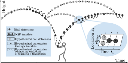
Figure 3: An example of ball detections, hypothesized ball locations when it is missed, and graph construction.

6 Experiments

In this section, we compare our results to those of several state-of-the-art multi-view ball-tracking algorithms [27, 28, 23], a monocular one [10], as well as two tracking methods that could easily be adapted for this purpose [30, 2].

We first describe the datasets we use for evaluation purposes. We then briefly introduce the methods we compare against and finally present our results.

6.1 Datasets

We use two volleyball, three basketball, and one soccer sequences, which we detail below.

Basket-1 and Basket-2

comprise a 4000- and a 3000-frame basketball sequences captured by 6 and 7 cameras, respectively. These synchronized 25-frame-per-second cameras are placed around the court. We manually annotated each 10th frame of Basket-1 and 500 consecutive frames of Basket-2 that feature flying ball, passed ball, possessed ball and ball out of play. We used the Basket-1 annotations to train our classifiers and the Basket-2 ones to evaluate the quality of our results, and vice versa.

Basket-APIDIS

is also a basketball dataset [26] captured by seven unsynchronized 22-frame-per-second cameras. A pseudo-synchronized 25-frame-per-second version of the dataset is also available and this is what we use. The dataset is challenging because the camera locations are not good for ball tracking and lighting conditions are difficult. We use 1500 frames with manually labeled ball locations provided by [23] to train the ball detector, and Basket-1 sequence to train the state classifier. We report our results on another 1500 frames that were annotated manually in [26].

Volley-1 and Volley-2

comprise a 10000- and a 19500-frame volleyball sequences captured by three synchronized 60-frame-per-second cameras placed at both ends of the court and in the middle. Detecting the ball is often difficult both because on either side of the court the ball can be seen by at most two cameras and because, after a strike, the ball moves so fast that it is blurred in middle camera images. We manually labeled each third frame in 1500-frame segments of both sequences. As before, we used one for training and the other for evaluation.

Soccer-ISSIA

is a soccer dataset [8] captured by six synchronized 25-frame-per-second cameras located on both sides of the field. As it is designed for player tracking, the ball is often out of the field of view when flying. We train on the 1000 frames and report results on another 1000.

In all these datasets, the apparent size of the ball is often so small that state-of-the-art monocular object tracker [30] was never able to track the ball reliably for more than several seconds.

6.2 Baselines

We use several recent multi-camera ball tracking algorithms as baselines. To ensure a fair comparison, we ran all publicly available approaches with the same set of detections, which were produced by the ball detector described in Sec. 5.2. We briefly describe these algorithms below.

• InterTrack [28] introduces an Integer Programming approach to tracking two types of interacting objects, one of which can contain another. Modeling the ball as being “contained” by the player in possession of it was demonstrated as a potential application. In [29], this approach is shown to outperform several multi-target tracking approaches [24, 17] for ball tracking task.

• RANSAC [23] focuses on segmenting ballistic trajectories of the ball and was originally proposed to track it in the Basket-APIDIS dataset. Approach is shown to outperform the earlier graph-based filtering technique of [22]. We found that it also performs well in our volleyball datasets that feature many ballistic trajectories. For the Soccer-ISSIA dataset, we modified the code to produce linear rather than ballistic trajectories.

• FoS [27] focuses on modeling the interaction between the ball and the players, assuming that long passes are already segmented. In the absence of a publicly available code, we use the numbers reported in the article for Basket-1-2-APIDIS and on Soccer-ISSIA.

• Growth [10] greedily grows the trajectories instantiated from points in consecutive frames. Heuristics are used to terminate trajectories, extend them and link neighbouring ones. It is based on the approach of [5] and shown to outperform approaches based on the Hough transform. Unlike the other approaches, it is monocular and we used as input our 3D detections reprojected into the camera frame.

To refine our analysis and test the influence of specific element of our approach, we also used the following approaches.

• MaxDetection. To demonstrate the importance of tracking the ball, we give the results obtained by simply choosing the detection with maximum confidence.

• KSP [2]. To demonstrate the importance of modeling interactions between the ball and the players, we use the publicly available KSP tracker to track only the ball, while ignoring the players.

• OUR-No-Physics. To demonstrate the importance of physics-based second-order constraints of Eq. 5, we turn them off.

• OUR-Two-States. Similarly, to demonstrate the impact of keeping track of many ball states, we assume that the ball can only be in one of two states, possession and free motion.

6.3 Metrics

Our method tracks the ball and estimates its state. We use a different metric for each of these two tasks.

Tracking accuracy

at distance $d$ is defined as the percent of frames in which the location of the tracked ball is closer than $d$ to the ground truth location. The curve obtained by varying $d$ is known as the “precision plot” [1]. When the ball is in_possession, its location is assumed to be that of the player possessing it. If the ball is reported to be not_present while it really is present, or vice versa, the distance is taken to be infinite.

Event accuracy

measures how well we estimate the state of the ball. We take an event to be a maximal sequence of consecutive frames with identical ball states. Two events are said to match if there are not more than $5$ frames during which one occurs and not the other. Event accuracy then is a symmetric measure we obtain by counting recovered events that matched ground truth ones, as well as the ground truth ones that matched the recovered ones, normalized by dividing it by the number of events in both sequences.

6.4 Comparative Results

We now compare our approach to the baselines in terms of the above metrics. As mentioned in Sec. 3.3, we obtain the players trajectories by first running the code of  [9] to compute the player’s probabilities of presence in each separate fame and then that of [2] to compute their trajectories. We first report accuracy results when these are treated as being correct, which amounts to fixing the $p_{i}^{j}$ in Eq. 8, and show that our approach performs well. We then perform joint optimization, which yields a further improvement.

Tracking and Event Accuracy.

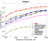
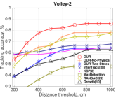
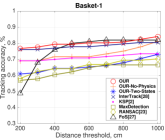
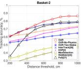
(a)	(b)	(c)	(d)
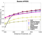
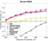
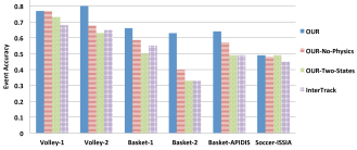
(e)	(f)	(g)

Figure 4: Comparative results. (a-f) OUR outperforms the other approaches in terms of ball accuracy, followed by the other methods that also model ball/player interaction, OUR-No-Physics, InterTrack, and FoS for larger values of $d$. (g) OUR also does best in terms of event accuracy.

Volley-1	Basket-1	Soccer-ISSIA

Figure 5: Visualisation of results on 3 10-second sequences from different sports. Cirlces indicate true ball location: empty circles correspond to free motion, filled circles indicate ball in_possession. Line indicates predicted ball locations: thick when predicted state is in_possession, thin otherwise. Best viewed in color.

As shown in Fig. 4(a-f), OUR complete approach, outperforms the others on all 6 datasets. Two other methods that explicitly model the ball/player interactions, OUR-No-Physics and InterTrack, come next. FoS also accounts for interactions but does markedly worse for small distances, probably due to the lack of an integrated second order model.

Volleyball.

The differences are particularly visible in the Volleyball datasets that feature both interactions with the players and ballistic trajectories. Note that OUR-Two-States does considerably worse, which highlights the importance of modeling the different states accurately.

Basketball.

The differences are less obvious in the basketball datasets where OUR-No-Physics and InterTrack, which model the ball/player interactions without imposing global physics-based constraints, also do well. This reflects the fact that the ball is handled much more than in volleyball. As a result, our method’s ability to also impose strong physics-based constraints has less overall impact.

Soccer.

On the soccer dataset, the ball is only present in about 75% of the frames and we report our results on those. Since the ball is almost never seen flying, the two states (in_possession and rolling) suffice, which explains the very similar performance of OUR and OUR-Two-States. KSP also performs well because in soccer occlusions during interactions are less common than in other sports. Therefore, handling them delivers less of a benefit.

Our method also does best in terms of event accuracy, among the methods that report the state of the ball, as shown in Fig. 4(g). As can be seen in Fig. 5, both the trajectory and the predicted state are typically correct. Most state assignment errors happen when the ball is briefly assigned to be in_possession of a player when it actually flies nearby, or when the ball is wrongly assumed to be in free motion, while is is really in_possession but clearly visible.

Simultaneous tracking of the ball and players.

All the results shown above were obtained by processing sequences of at least 500 frames. In such sequences, the people tracker is very reliable and makes few mistakes. This contributes to the quality of our results at the cost of an inevitable delay in producing the results. Since this could be damaging in the live-broadcast situation, we have experimented with using shorter sequences. We show here that simultaneously tracking the ball and the players can mitigate the loss of reliability of the people tracker, albeit to a small extent.

Metric	MODA [14],%	Tracking acc. @ 25 cm,%
50	94.1 / 93.9 / 0.26	69.2 / 67.2 / 2.03
75	94.5 / 94.2 / 0.31	71.4 / 69.4 / 2.03
100	96.5 / 96.3 / 0.21	72.5 / 71.0 / 1.41
150	97.2 / 97.1 / 0.09	73.8 / 73.0 / 0.82
200	97.3 / 97.4 / 0.00	74.1 / 74.1 / 0.00

(a)                            (b)

Table 2: Tracking the ball given the players’ locations vs. simultaneous tracking of the ball and players. The three numbers in both columns correspond to simultaneous tracking of the players and ball / sequential tracking of the players and then the ball / improvement, as function of the lengths of the sequences. (a) People tracking accuracy in terms of the MODA score. (b) Ball tracking accuracy.

As shown in Tab. 2 for the Volley-1 dataset, we need 200-long frames to get the best people tracking accuracy when first tracking the people by themselves first, as we did before. As the number of frames decreases, the people tracker becomes less reliable but performing the tracking simultaneously yields a small but noticeable improvement both for the ball and the players. The case of Fig. 1 is an example of this. We identified 3 similar cases in 1500 frames of the volleyball sequence used for the experiment.

7 Conclusion

We have introduced an approach to ball tracking and state estimation in team sports. It uses Mixed Integer Program that allows to account for second order motion of the ball, interaction of the ball and the players, and different states that the ball can be in, while ensuring globally optimal solution. We showed our approach on several real-world sequences from multiple team sports. In future, we would like to extend this approach to more complex tasks of activity recognition and event detection. For this purpose, we can treat events as another kind of objects that can be tracked through time, and use interactions between events and other objects to define their state.

References

- [1] B. Babenko, M. Yang, and S. Belongie. Robust Object Tracking with Online Multiple Instance Learning. IEEE Transactions on Pattern Analysis and Machine Intelligence, 33(8):1619–1632, 2011.
- [2] J. Berclaz, F. Fleuret, E. Türetken, and P. Fua. Multiple Object Tracking Using K-Shortest Paths Optimization. IEEE Transactions on Pattern Analysis and Machine Intelligence, 33(11):1806–1819, September 2011.
- [3] L. Breiman. Random Forests. Machine Learning, 2001.
- [4] B. Chakraborty and S. Meher. A real-time trajectory-based ball detection-and-tracking framework for basketball video. Journal of Optics, 42(2):156–170, 2013.
- [5] H.-T. Chen, H.-S. Chen, and S.-Y. Lee. Physics-based ball tracking in volleyball videos with its applications to set type recognition and action detection. In International Conference on Acoustics, Speech, and Signal Processing, 2007.
- [6] H.-T. Chen, M.-C. Tien, Y.-W. Chen, W.-J. Tsai, and S.-Y. Lee. Physics-based ball tracking and 3D trajectory reconstruction with applications to shooting location estimation in basketball video. Journal of Visual Communication and Image Representation, 20:204–216, 2009.
- [7] C. Direkoǧlu and N. O’Connor. Team Activity Recognition in Sports. In European Conference on Computer Vision, pages 69–83, October 2012.
- [8] T. D’Orazio, M. Leo, N. Mosca, P. Spagnolo, and P. L. Mazzeo. A Semi-Automatic System for Ground Truth Generation of Soccer Video Sequences. In International Conference on Advanced Video and Signal Based Surveillance, pages 559–564, 2009.
- [9] F. Fleuret, J. Berclaz, R. Lengagne, and P. Fua. Multi-Camera People Tracking with a Probabilistic Occupancy Map. IEEE Transactions on Pattern Analysis and Machine Intelligence, 30(2):267–282, February 2008.
- [10] G. Gomez, P. López, D. Link, and B. Eskofier. Tracking of Ball and Players in Beach Volleyball Videos. PLoS ONE, 2014.
- [11] A. Gupta, P. Srinivasan, J. Shi, and L. S. Davis. Understanding Videos, Constructing Plots Learning a Visually Grounded Storyline Model from Annotated Videos. In Conference on Computer Vision and Pattern Recognition, pages 2012–2019, 2009.
- [12] Gurobi. Gurobi Optimizer, 2012. http://www.gurobi.com/.
- [13] M. Hearst, S. Dumais, E. Osuna, J. Platt, and B. Scholkopf. Support Vector Machines. IEEE Intelligent Systems and their Applications, 13(4):18–28, 1998.
- [14] R. Kasturi, D. Goldgof, P. Soundararajan, V. Manohar, J. Garofolo, M. Boonstra, V. Korzhova, and J. Zhang. Framework for Performance Evaluation of Face, Text, and Vehicle Detection and Tracking in Video: Data, Metrics, and Protocol. IEEE Transactions on Pattern Analysis and Machine Intelligence, 31(2):319–336, February 2009.
- [15] K. Kim, D. Lee, and I. Essa. Detecting Regions of Interest in Dynamic Scenes with Camera Motions. In Conference on Computer Vision and Pattern Recognition, 2012.
- [16] T. Lan, L. Sigal, and G. Mori. Social Roles in Hierarchical Models for Human Activity Recognition. In Conference on Computer Vision and Pattern Recognition, July 2012.
- [17] L. Leal-taixe, M. Fenzi, A. Kuznetsova, B. Rosenhahn, and S. Savarese. Learning an Image-Based Motion Context for Multiple People Tracking. In Conference on Computer Vision and Pattern Recognition, 2014.
- [18] M. Leo, N. Mosca, P. Spagnolo, P. Mazzeo, T. D’Orazio, and A. Distante. Real-Time Multiview Analysis of Soccer Matches for Understanding Interactions Between Ball and Players. In Conference on Image and Video Retrieval, 2008.
- [19] J. Liu, P. Carr, R. T. Collins, and Y. Liu. Tracking Sports Players with Context-Conditioned Motion Models. In Conference on Computer Vision and Pattern Recognition, pages 1830–1837, 2013.
- [20] P. Lucey, A. Bialkowski, P. Carr, S. Morgan, I. Matthews, and Y. Sheikh. Representing and Discovering Adversarial Team Behaviors Using Player Roles. In Conference on Computer Vision and Pattern Recognition, 2013.
- [21] Y. Ohno, J. Miura, and Y. Shirai. Tracking Players and Estimation of the 3D Position of a Ball in Soccer Games. In International Conference on Pattern Recognition, 2000.
- [22] P. Parisot and C. D. Vleeschouwer. Graph-Based Filtering of Ballistic Trajectory. In International Conference on Multimedia and Expo, 2011.
- [23] P. Parisot and C. D. Vleeschouwer. Consensus-Based Trajectory Estimation for Ball Detection in a Calibrated Cameras System. EURASIP Journal on Image and Video Processing, 2015. Code available at http://sites.uclouvain.be/ispgroup/index.php/Softwares/APIDIS.
- [24] H. Pirsiavash, D. Ramanan, and C. Fowlkes. Globally-Optimal Greedy Algorithms for Tracking a Variable Number of Objects. In Conference on Computer Vision and Pattern Recognition, June 2011.
- [25] J. Ren, J. Orwell, G. A. Jones, and M. Xu. Real-Time Modeling of 3D Soccer Ball Trajectories from Multiple Fixed Cameras. IEEE Transactions on Circuits and Systems for Video Technology, 18(3):350–362, 2008.
- [26] C. D. Vleeschouwer, F. Chen, D. Delannay, C. Parisot, C. Chaudy, E. Martrou, A. Cavallaro, et al. Distributed Video Acquisition and Annotation for Sport-Event Summarization. New European Media, 8, 2008.
- [27] X. Wang, V. Ablavsky, H. BenShitrit, and P. Fua. Take your Eyes Off the Ball: Improving Ball-Tracking by Focusing on Team Play. Computer Vision and Image Understanding, 119:102–115, 2014.
- [28] X. Wang, E. Turetken, F. Fleuret, and P. Fua. Tracking Interacting Objects Optimally Using Integer Programming. In European Conference on Computer Vision, September 2014.
- [29] X. Wang, E. Turetken, F. Fleuret, and P. Fua. Tracking Interacting Objects Using Intertwined Flows. IEEE Transactions on Pattern Analysis and Machine Intelligence, submitted, 2015.
- [30] K. Zhang, L. Zhang, and M. H. Yang. Real-Time Compressive Tracking. In European Conference on Computer Vision, 2012.
- [31] Y. Zhang, H. Lu, and C. Xu. Collaborate Ball and Player Trajectory Extraction in Broadcast Soccer Video. In International Conference on Pattern Recognition, 2008.
- [32] G. Zhu, Q. Huang, C. Xu, Y. Rui, S. Jiang, W. Gao, and H. Yao. Trajectory based event tactics analysis in broadcast sports video. In ACM Multimedia, pages 58–67, 2007.