What statistics can tell us about strategy in tennis

Abstract

In this paper we analyse tiebreak results from some tennis players in order to investigate whether we are able to identify a non-aleatory distribution of the points in this crucial moment of the game. We compared the observed results with a binomial distribution considering that the probabilities of winning or losing a point are equal. Using a $\chi^{2}$ test we found that, excepting some players, the greatest part of the results agrees with our hypothesis that the points in tiebreaks are merely aleatory.

Keywords: Sports, $\chi^{2}$ Test, Binomial Distribution

1 Introduction

A recurrent question in a signal analysis is whether it is a true signal or just a noise [1, 2]. This question arises, for example, when we are analysing a tomography or X-ray picture [3] or searching for a new particle like Higgs boson [4]. In these cases different statistical tests are made and usually the discussion is how many standard deviations we can accept or reject a given hypothesis. Statistical analysis of experimental data are made since the first years of physics and engineering courses [5]. The connection of classroom problems with daily problems [6, 7] may be more stimulating than, for example, roll many dice hundreds times to see in practice a binomial distribution. The aim of this paper is to investigate whether the points in a tiebreak originate from a statistical fluctuation and are randomly decided.

A tennis match is divided in sets and games. To win a set the player should complete six games with at least two games of difference from the other player (6x0, 6x1, $\dots$, 6x4). In the case of a player with six games and the other with five, it is played one more game and then it may happen two things: if the player with six games wins the game then the set ends in 7x5. If the player loses the game then the set is tied and they will play a tiebreak . During the tiebreak, the player who wins the first seven points with at least two points of difference of the other player wins the game and the set. If necessary, the tiebreak continues until the minimum difference of two points is achieved.

In this paper we collected results from tiebreaks of several players. We then plotted in a histogram the difference of points, where positive values mean victories and negative losses. These histograms are compared with a theoretical binomial distribution, constrained to the tennis rules described in the last paragraph, but considering equal probabilities of winning or losing a point. We performed a $\chi^{2}$ test to have an objective parameter to say if the observed and calculated results are statistically different.

The paper is organized as follows. In section 2 we explain the criterium we used to select the players and the $\chi^{2}$ test. In section 3 we compare the observed results and our theoretical prediction. Finally, in section 4 we summarize and give our conclusions.

2 Methods

Analysing the conditions which may lead to a tiebreak we could consider two main reasons. The first one: both players may have a very similar game. Then, considering that the serve can really be considered as an advantage, we will have in this condition a very favorable condition for a tiebreak (every game of serve the player who is serving wins the game). The second reason usually occurs when one of the players has an amazing serve. Normally, this condition comes essentially from a very big height (exceptions to this fact may be found). Then, thanks to the height the agility of the player is seriously compromised, which makes that in one hand the tall player has a low probability to win the game when his opponent is serving, but on the other hand the opponent rarely can obtain a good return of the big serve. A good example for this second reason is Ivo Karlovic (211 cm) from Croatia. However, despite of what reason caused the tiebreak, the fact is: when the match goes to a tiebreak, in that moment the match was very balanced. Thus, it is not strange to think that each point could go randomly to any of the players.

In order to investigate tiebreak results, we selected the top ten players according to ATP (Professional Tennis Association) website in the last week of October, 2015. For the analysis we also included the player Ivo Karlovic, as his games usually go to a tiebreak. The tiebreak results were mainly extract from gambling sites, where we may find detailed results.

In 1 we plotted a binomial distribution of a tiebreak in tennis considering that the probability to win, or lose, a point in the tiebreak is 0.5.

Figure 1: Theoretical result for the probability to have a result from -7 to 7 in a tiebreak considering that the probability to win(lose) a point is 0.5. Horizontal axis is the difference of points from a given and other players. Positive values mean victories and negative losses.

We calculated the $\chi^{2}$ quantity in order to compare the expected results with the observed ones. The $\chi^{2}$ variable is defined as:

$$\chi^{2}=\sum_{-7}^{7}\frac{(y_{i}^{(O)}-y_{i}^{(E)})^{2}}{y_{i}^{(E)}},$$ (1)

where $y_{i}^{(O)}$ and $y_{i}^{(E)}$ are, respectively, the observed and expected number of events. The sum should be performed over all values. The expected number of events is simply given by $Np_{i}$, where $N$ is the total number of events and $p_{i}$ ($i=-7,\dots,7$) is the probability for result $i$ to occur (see Fig. 1). Defining $F=F(\chi^{2})$ as the probability density function for eleven degrees of freedom, we may write, respectively, the probability of finding a smaller and a greater value than a given $\chi^{2}$ as

$$P_{<}=\int_{0}^{\chi_{<}^{2}}F(\chi^{2})d\chi^{2},\;\;\;\;\;P_{>}=\int_{\chi_{>}^{2}}^{\infty}F(\chi^{2})d\chi^{2}.$$ (2)

Here, we will consider that the observed values agree with our theoretical result if the calculated $\chi^{2}$ stays inside the interval $\chi_{<}^{2}<\chi^{2}<\chi_{>}^{2}\equiv 4.575<\chi^{2}<19.675$, which corresponds to $P_{<}=0.05$ and $P_{>}=0.95$.

3 Results

In this section we will compare our theoretical result with some observed data. Fig. 2 shows the expected results, given by $Np_{i}$ (for Karlovic $N=274$) and represented by open circles, compared to the observed ones. Not only the structure of the results are very similar, but also the values in each channel. The calculated $\chi^{2}$ is 10.6, which is inside the interval mentioned in the last section indicating that both results are statistically equivalent. This means that despite the big serve from Karlovic his results in tiebreak are close to a completely random situation.

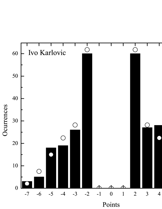
Figure 2: Histogram of Ivo Karlovic results. The bars are a total of 274 collected data and the open circles are our theoretical results. The agreement between both results are very good giving a $\chi^{2}=10.6$. This result means that despite the great serve from Karlovic, the probability of winning (or losing) a point is close to 50 %.

Figure 3 shows the results from Roger Federer. We can immediately note the large difference from the theoretical and observed results. This is clearly a non-aleatory result with a $\chi^{2}$ exceeding by far the upper limit of 19.675. Roger Federer is one of the greatest tennis players of all time and this figure may demonstrate it. Tennis is a very mental game with moments of extreme pressure (tiebreaks, for example). A crucial moment occurs when the point can define the game, the set, or the match. The top tennis players have the capacity to increase considerably their concentration and tennis level in these moments. The courage to hit a drop shot or a ball down the line in a delicate moment avoiding the opponent to win the point is a quality that is not shared by all players.

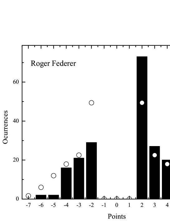
Figure 3: Histogram of Roger Federer results. Same as figure 2 for 219 data and a $\chi^{2}=39.3$. This is a typical figure of non-aleatory results.

Table 1 shows the calculated $\chi^{2}$ for the top ten players at the moment we were writing this paper (note that the ranking changes every week) and Ivo Karlovic, who has the biggest number of aces in history and a large number of tiebreaks. In order to agree with the theoretical prediction (50 % of probability to win or lose a point in tiebrak) the $\chi^{2}$ should stay inside the interval $[4.575,19.675]$. As we can see, Djokovic, Murray, Wawrinka, Ferrer, Tsonga and Karlovic agree with an aleatory result. Note that almost more than half of the top ranked players have practically random tiebreak results. If we consider lower rankings the number of players who agree with our hypothesis increases considerably.

Player	$\chi^{2}$	Data
Novak Djokovic	19.0	181
Roger Federer	39.3	219
Andy Murray	14.6	168
Stan Wawrinka	11.4	197
Tomas Berdych	21.6	199
Rafael Nadal	29.3	163
Kei Nishikori	23.7	115
David Ferrer	9.1	151
Jo-Wilfried Tsonga	11.0	220
Milos Raonic	31.9	260
Ivo Karlovic	10.6	274

Table 1: Calculated $\chi^{2}$-values for several players. The last column is the number of collected data. In order to be statistically equivalent to a random result, $\chi^{2}$ should stay inside $4.575<\chi^{2}<19.675$. In this table, the values larger than 19.675 correspond to more victories than that predicted by our model.

4 Conclusion

We could see from our calculations that half of the top ten players and the player who has the greatest number of aces in history (Karlovic) display a tiebreak result that is in agreement with our hypothesis of aleatory points. Definitely, this is not a statistical accident. The agreement with our prediction just tell that the strategy used by these players to play tiebreaks is returning the same result as the coin thrown in the beginning of the match to decide which player serves first. Besides not an easy task, the coach of these players could at least adopt a strategy which could arrive in a result different of 50 %. Considering lower rankings the number of players who agree with our hypothesis increases considerably.

As written in the introduction, statistical analysis is a topic explored in the first years of undergraduate physics or engineering courses. A contact with a real problem where it is possible to analyse the data of your favorite team or player is by far more exciting than spend an hour (or more) rolling many dice to see in practice a binomial distribution. Variations of the problem treated here may be easily extended to other sports like, e.g. football.

References

References

- [1] Helene, O. Upper limit of peak area Nucl. Instrum. Methods Phys. Res. 212 319-22 (1983)
- [2] Razak, M. M. A. Detection and extraction of weak signals buried in noise Am. J. Phys. 77 1061-65 (2009)
- [3] Mylott, E.; Klepetka, R.; Dunlap, J. C. and Widenhorn, R. An easily assembled laboratory exercise in computed tomography Eur. J. Phys. 32 1227-35 (2011)
- [4] ATLAS Collaboration Observation of a new particle in the search for the Standard Model Higgs boson with the ATLAS detector at the LHC Phys. Lett. B 716 1-29 (2012); CMS Collaboration Observation of a new boson at a mass of 125 GeV with the CMS experiment at the LHC Phys. Lett. B 716 30 (2012)
- [5] Peterlin, P. Data analysis and graphing in an introductory physics laboratory: spreadsheet versus statistics suite Eur. J. Phys. 31 919-31 (2010)
- [6] Helene, O. and Yamashita, M. T. The force, power and energy of the 100-meter sprint Am. J. Phys. 78 307-9 (2010); Helene, O. and Yamashita, M. T. A unified model for the long and high jump Am. J. Phys. 73 906-8 (2005)
- [7] Helene, O. and Yamashita, M. T. Understanding the tsunami with a simple model Eur. J. Phys. 27 855-63 (2006)