Rotating turbulence under “precession-like” perturbation

Abstract

The effects of changing the orientation of the rotation axis on homogeneous turbulence is considered. We perform direct numerical simulations on a periodic box of $1024^{3}$ grid points, where the orientation of the rotation axis is changed (a) at a fixed time instant (b) regularly at time intervals commensurate with the rotation time scale. The former is characterized by a dominant inverse energy cascade whereas in the latter, the inverse cascade is stymied due to the recurrent changes in the rotation axis resulting in a strong forward energy transfer and large scale structures that resemble those of isotropic turbulence.

1 Introduction

Turbulence subjected to rotation is a commonly occurring phenomenon in geophysical and astrophysical flows, such as those in the oceans and atmospheres of planetary bodies. The effects of rotation on decaying homogeneous turbulence is typically studied by considering either an isotropic or anisotropic state as the initial condition camb97 ; mans91 . In direct numerical simulations, different external forcing mechanisms have also been considered in order to vary the degree of anisotropy and the typical correlation time SM14 ; SM15 of the flow. In most cases, it is customary to fix the orientation of the rotation axis. The general consensus is that when rotation is strong enough, the forward energy cascade from the large scales to the small scales is inhibited and an inverse cascade develops resulting in a quasi-two-dimensional behavior characterized by columnar structures along the fixed rotation axis Pouquet2010 ; sen12 . The dominance of the inverse energy cascade entails the presence of a large scale energy sink in order to reach stationarity xia11 . In this work, we consider the effects of instantaneous changes to the orientation of the rotation axis on homogeneous turbulence.

The interest in the orientation of rotation axis is engendered by the phenomenon of precession, which is the rotational motion of the spin axis of a rotating body kida11 . Even a weakly precessing container is known to sustain turbulence at a sufficiently large Reynolds number, due to viscous forces on the container walls goto07 ; Malkus . For instance, the turbulent convection of liquid metals in the Earth’s outer core is influenced by its slow precession. However details of the flow structure and the energy transfer dynamics in turbulence subjected to precession remain unclear partly due to the fact that experiments as well as simulations are difficult to conduct goto14 .

As a recourse, we compare the spectral transfer properties of a system perturbed by changing the orientation of the axis at a given time instant and consequently allowed to relax, with another system which is perturbed at regular time intervals by repeatedly changing the orientation of the axis. We show that the latter has different large scale properties and transfer dynamics as compared with the former. The remainder of this work is organized as follows. In Sec. 2 we briefly review the equations involved, simplifying assumptions made and details about the simulations performed. Results are given in Sec. 3, with three subsections which focus respectively on (3.1) the evolution of the kinetic energy and dissipation rate, (3.2) energy spectra and flux and (3.3) large scale structure evolution. In Sec. 4 we summarize our results and discuss briefly the possible implications of this work.

2 Numerical method

The fluctuating velocity $\mathbf{u}(\mathbf{x},t)$ for a constant density flow in the co-ordinate system rotating with angular velocity $\mathbf{\Omega}\equiv\mathbf{\Omega}(t)$ is given by gspan

$$\mkern-18.0mu\!\!\!\frac{\partial\mathbf{u}}{\partial t}+\mathbf{u}\cdot\mathbf{\nabla}\mathbf{u}+2\mathbf{\Omega}\times\mathbf{u}+\frac{d(\mathbf{\Omega}\times\mathbf{r})}{dt} =$$

$$-\mathbf{\nabla}p+\mathbf{f}+\nu\mathbf{\Delta}\mathbf{u}-\gamma\mathbf{\Delta}^{-1}\mathbf{u}\;,$$ (1)

where $\mathbf{f}$ is the forcing stirring the fluid, $\nu$ is the constant viscosity, $\gamma$ is the large scale damping constant needed to remove energy at large scale and $\mathbf{\Delta}$ denotes the Laplacian operator. The distance of the fluid particle from the rotation axis which precesses around a fixed axis is $|\mathbf{r}|=r$. In Eq. 1 the pressure $p$ accounts for the centrifugal acceleration $\mathbf{\Omega}\times(\mathbf{\Omega}\times\mathbf{r})$ in the usual manner. In Eq. 1, the precession term $d(\mathbf{\Omega}\times\mathbf{r})/dt\sim\Omega L/\tau_{p}$, where $\tau_{p}$ is the precession time scale. If $\tau_{p}$ is large enough, the precession term is negligible compared to the (time dependent) Coriolis term since $\Omega L/\tau_{p}\ll\Omega L/T_{E}$ where $L$ and $T_{E}$ denote the integral scale and the large eddy timescale of the flow. Neglecting the precession term assuming $\tau_{p}\gg T_{E}$ is a reasonable approximation in many geodynamo applications which are characterized by large precession time periods nore ; triana . Another relevant scenario is that of a sudden change in the orientation of the rotation axis at a given time instant, say at $t=0$, as a sort of an instantaneous perturbation. In this case, one might expect that neglecting the non-homogeneous term becomes less and less important for the late-time dynamics, i.e. for $t\gg 0$. Accordingly, we solve the following equation numerically under the assumption that the precession term $d(\mathbf{\Omega}\times\mathbf{r})/dt$ can be neglected:

$$\frac{\partial\mathbf{u}}{\partial t}+\mathbf{u}\cdot\mathbf{\nabla}\mathbf{u}+2\mathbf{\Omega}\times\mathbf{u}=-\mathbf{\nabla}p+\mathbf{f}+\nu\mathbf{\Delta}\mathbf{u}-\gamma\mathbf{\Delta}^{-1}\mathbf{u}\;.$$ (2)

Equation 2 is valid for weakly precessing flows which are characterized by a large precession time scale $\tau_{p}$. Alternatively, for sub-volumes of the flow close to the rotation axis, such that $|d(\mathbf{\Omega}\times\mathbf{r})/dt|\sim\Omega r/\tau_{p}\to 0$ as $r\to 0$, the precession term can be neglected in comparison to the Coriolis term. The aim of this paper is to understand the evolution of the rotating flow under such sudden changes to the orientation of the rotation axis. It also allows us to assess the robustness and universality of the large scale structures in strongly rotating turbulence. We solve Eq. 2 using a Fourier pseudo-spectral method for spatial discretization and a second order Adams-Bashforth scheme for the time integration. The domain is a periodic cube with edge length $L_{0}=2\pi$ with $N$ grid points to a side. The smallest wave number in the domain is $k_{0}=1$. The stochastic forcing applied to a shell around the forcing wave number $k_{f}/k_{0}=4$ is based on a second-order Ornstein-Ulhenbeck process saw91 . The hypo-viscous mechanism used to damp the large scales is applied to wave numbers $k\in[0.5,2.5]$, with a large scale damping constant $\gamma=0.1$ (refer Eqs. 1 and 2). Simulations wherein energy was depleted from different large scale ranges were also performed to test if the large scale properties systematically depend on the particular choice of wave numbers at which the energy was removed. This issue of choice of low wave numbers from which energy is depleted is further discussed in 3.3. Aliasing errors from the nonlinear term are effectively controlled by removing all coefficients with wave number magnitude greater than $k_{max}/k_{0}=N/3$.

3 Results and Analysis

Figure 1: Schematic of the orientation of the rotation vector $\mathbf{\Omega}$ in the $X$-$Y$ plane for simulations (left) R1 and (right) R2, $\Delta\theta=\pi/4$. In run R1 $\mathbf{\Omega}$ is rotated only at $t=0$ while in run R2 it is rotated at $t_{i}/\tau_{\Omega}=10i$, $i=0,1,2,\ldots$

We present results from two direct numerical simulations, at grid resolution $1024^{3}$ and constant rotation magnitude $\Omega=10$. The rotation vector $\mathbf{\Omega}$ lies in the $X$-$Y$ plane and is defined by the angle $\theta$ it makes with the $X$-axis (Fig. 1). A rotating, stationary flow at $1024^{3}$, $\Omega=10$, $\theta=0$ is used as the initial condition ($t=0$) for both the simulations. Statistical stationarity for $t\leq 0$ is achieved using the same large scale friction mechanism that is used in simulations R1 and R2.

Table 1: Initial and final values of Rossby numbers and related parameters in the $1024^{3}$, $\Omega=10$ simulations. The forcing wave number $k_{f}/k_{0}=4$. Large scale dissipation is applied to wave number $k\in[0.5,2.5]$. Notes: (1) $T_{E}^{0}\equiv K(0)/\epsilon(0)$ is the turbulence time scale at $t=0$. (2) $\tau_{\eta}=(\nu/\epsilon)^{1/2}$ is the Kolmogorov time scale and $\eta=(\nu^{3}/\epsilon)^{1/4}$ is the Kolmogorov length scale.

	$t=0$	R1	R2
$t/T_{E}^{0}$	$0.0$	$11.75$	$6.95$
${Ro}_{T}=\epsilon/(2K\Omega)$	$0.0063$	$0.0050$	$0.0218$
$Ro^{\omega}=1/(2\tau_{\eta}\Omega)$	$1.4231$	$1.3151$	$1.6863$
$k_{\Omega}\eta$	$0.2083$	$0.2344$	$0.1615$

Simulation R1 is performed using $\theta=\pi/4$, while R2 is performed by instantaneously incrementing $\theta$ by $\Delta\theta=\pi/4$ every $10\tau_{\Omega}$, where $\tau_{\Omega}\equiv 1/\Omega$ is the rotation time scale. A schematic of the orientation of $\mathbf{\Omega}$ in the two runs is depicted in Fig. 1. A conventional measure of the strength of the rotation is given by comparing the rotation time scale to the turbulence time scale ($K/\epsilon$), giving the turbulent Rossby number $Ro_{T}\equiv\epsilon/(2K\Omega)$. Here $K$ is the kinetic energy and $\epsilon$ is the mean dissipation and are defined in Eqs. 3 and 4 respectively. The definitions of the Rossby numbers including initial and final values of these quantities are summarized in Tab. 1. The initial large eddy time scale is defined as $T_{E}^{0}\equiv K/\epsilon$ at $t=0$. The Rossby numbers for run R2 at the end of the simulation show an increase compared to their initial values showing that the effect of rotation has possibly decreased. In contrast, for run R1 the turbulent Rossby number $Ro_{T}$ and the micro-Rossby number $Ro^{\omega}$ have decreased indicating that effects of rotation are still significant. A characteristic wave number of rotation ($k_{\Omega}$) which delimits the region of the spectrum where rotation effects are important ($k<k_{\Omega}$) is given by $k_{\Omega}=({\Omega}^{3}/\epsilon)^{1/2}$ zee94 . The non-dimensional rotation wave number $k_{\Omega}\eta\sim 1$ in the simulations (Tab. 1), indicating that the rotation effects extend to the viscous scales in the flow.

3.1 Energy and dissipation

Figure 2: Evolution of kinetic energy (left) and dissipation (right) in normalized time, compared with respective values at $t=0$. Solid curves corresponds to run R1, curves with symbols ($\bigtriangleup$) correspond to run R2. Dashed curves show histories of $K(t)$ and $\epsilon(t)$ prior to start ($t<0$) of the perturbation. Time axis is normalized by large eddy time scale at $t=0$ ($T_{E}^{0}$) in bottom horizontal axis and by rotation time scale ($\tau_{\Omega}$) in top horizontal axis.

The mean turbulent kinetic energy and dissipation provide important global measures of the state of the turbulence under rotation. In homogeneous turbulence, the mean turbulent kinetic energy is defined as

$$K=\frac{1}{2}\Big{\langle}\sum_{i=1}^{3}u_{i}^{2}\Big{\rangle}\;,$$ (3)

and the mean dissipation rate is given by

$$\epsilon=2\nu\Big{\langle}\sum_{i,j=1}^{3}\frac{\partial u_{i}}{\partial x_{j}}\frac{\partial u_{j}}{\partial x_{i}}\Big{\rangle}\;,$$ (4)

where, $\langle\cdot\rangle$ denote space averages. In Fig. 2 we show the evolution of these quantities normalized by their initial values. Despite the considerable statistical variability, it is clear that the kinetic energy initially decreases for simulation R1, but subsequently increases with time. On the other hand, the energy for simulation R2 drops in the early stages and then remains nearly constant at a value well below that of R1. The steep drop in the energy at early times is accompanied by a sharp increase in mean dissipation. The dissipation rates then drop to nearly constant values with that of simulation R2 stabilizing at a value larger than that of R1. Furthermore, the time histories of energy and dissipation prior to the start of the perturbation ($t<0$ in Fig. 2) indicate that the initial changes in energy and dissipation caused by the change in orientation of $\mathbf{\Omega}$ are significant. The previous observations indicate that a single perturbation in the form of an instantaneous change to the orientation of the rotation axis results in a slow recovery of the “universal” inverse energy transfer mechanism. In contrast, if the system is subjected to such perturbations repeatedly, the inverse energy transfer is eventually destroyed as the dynamical reconstruction of the large scale structures is too slow to survive. Indeed, the dissipation of run R2 attains a quasi-stationary state which is higher than its initial value, while its energy stabilizes at a lower value. This indicates a net energy transfer from large scales to the small scales in simulation R2.

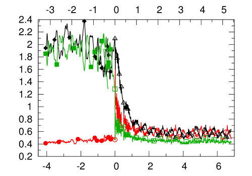
Figure 3: (Color online) Evolution of the three components of the turbulent kinetic energy $\langle u_{\alpha}^{2}\rangle,\;\alpha=1,2,3$ as a function of normalized time for run (left) R1 and (right) R2. Open symbols ($\Circle$), ($\bigtriangleup$) and ($\square$) correspond to $\langle u_{1}^{2}\rangle$, $\langle u_{2}^{2}\rangle$ and $\langle u_{3}^{2}\rangle$ respectively in the simulations. Closed symbols ($\CIRCLE$), ($\blacklozenge$) and ($\blacksquare$) correspond to time histories ($t<0$) of $\langle u_{1}^{2}\rangle$, $\langle u_{2}^{2}\rangle$ and $\langle u_{3}^{2}\rangle$ respectively prior to the start of the perturbation. Time axis is normalized by large eddy time scale at $t=0$ ($T_{E}^{0}$) in bottom horizontal axis and by rotation time scale ($\tau_{\Omega}$) in top horizontal axis.

The evolution of the Cartesian components of the turbulent kinetic energy are indicative of large scale anisotropy in the flow. Figure 3 compares the variance of the velocity components $\langle u_{\alpha}^{2}\rangle$ in the two simulations. Prior to the start of the perturbations, the velocity fluctuations perpendicular to the rotation axis ($\theta=0$ for $t<0$ in Fig. 1) are dominant due to an inverse energy cascade in the $Y$-$Z$ plane. The instantaneous rotation of $\mathbf{\Omega}$ at $t=0$ disrupts the spectral transfer to the largest scales in the $Y$-$Z$ plane. With time, in run R1 an inverse cascade in the plane normal to the new rotation axis is established resulting in increasing energy in the $Z$-direction. The variance of velocity components in the $X$ and $Y$ directions evolve similarly at a lower value than the $Z$ component. Whereas in run R2, the disruption of the inverse cascade at $t=0$ is sustained by the regular change in the orientation of the rotation axis. As a result, the energy components reach a stationary isotropic state.

3.2 Energy spectra and flux

Figure 4: Energy spectrum normalized by rotation scaling at different times for (left) simulation R1 and (right) simulation R2. Symbols $A$-$G$ correspond to $t/T_{E}^{0}=1/4,1/2,1,2,3,4,5$ respectively. Curve with (long) dashes corresponds to $t=0$. Dashed horizontal lines at $C_{\Omega}=1.75$ for reference. Forcing wave number magnitude $k_{f}/k_{\Omega}\approx 0.1$ for simulations R1 and R2 at all times shown. Inset shows blow-up of the intermediate scale range $k_{f}\leq k\leq k_{\Omega}$ at late-time. Dashed horizontal line at $C_{\Omega}=1.75$ corresponds to $k^{-2}$ scaling, while long-dashed line corresponds to Kolmogorov $-5/3$ spectrum krs95 .

In the rotation-modified inertial range, theoretical arguments zhou95 suggest that for $k_{f}\ll k\ll k_{\Omega}$ the energy spectrum is of the form

$$E(k)=C_{\Omega}(\epsilon\Omega)^{1/2}k^{-2}\;,$$ (5)

where the constant $C_{\Omega}=1.22-1.87$ zhou95 . In Fig. 4 we show the development of the compensated energy spectrum $E(k)(\epsilon\Omega)^{-1/2}k^{2}$ at different times for both simulations R1 and R2. The energy at low wave numbers ($k<k_{f}$) initially decreases ($t/T_{E}^{0}<1$) and then increases for run R1 whereas the energy at the largest scales in run R2 monotonically decreases with time. These results are consistent with energy evolution trends of the two simulations shown in Fig. 2. At the intermediate wave numbers $k_{f}\ll k\ll k_{\Omega}$, run R1 exhibits a $k^{-2}$ behavior with an inertial range plateau of $C_{\Omega}=1.75$. In contrast, run R2 shows a greater tendency towards a transition to the classical $k^{-5/3}$ scaling in the inertial range which is typical of flows without strong rotation min12 . On the other hand, the energy at the high wave numbers ($k>k_{\Omega}$) is greater in run R2 than in run R1, indicating a stronger forward cascade in the former. The results confirm that the transfer dynamics in the case with “precession-like” perturbations are inherently different than the case with a fixed rotation axis.

Figure 5: Spectral flux (Eq. 6) normalized by kinetic energy at different times for (left) run R1 and (right) run R2. Different curves correspond to different instants of time (refer Fig. 4). Dashed horizontal line at $0$ for reference. The maximum (negative) amplitude of flux increases with time (curves $A$-$G$) for run R2. Positive spectral flux corresponds to an inverse energy cascade while negative flux indicates a forward cascade (see Eq. 6).

The direction of energy transfer can be conveniently studied by examining the contribution of the nonlinear terms in Eq. 2 to the rate of change of energy in $k$-space. Following MY.II we define the spectral flux as

$$\Pi(k)=\!\!\int\displaylimits_{0}^{k}\!{\textrm{Im}\Big{\langle}{k^{{}^{\prime}}_{m}P_{ij}(\mathbf{k^{{}^{\prime}}})\hat{u}_{i}^{*}(\mathbf{k^{{}^{\prime}}})\mkern-18.0mu\!\!\!\int\displaylimits_{\mathbf{k^{{}^{\prime}}}=\mathbf{p}+\mathbf{q}}{\mkern-18.0mu\hat{u}_{j}(\mathbf{p})\hat{u}_{m}(\mathbf{q})}}\Big{\rangle}d\mathbf{p}\;dk^{{}^{\prime}}}.$$ (6)

Here $\textrm{Im}(\cdot)$ denotes imaginary part of $(\cdot)$, overcarets represent Fourier coefficients, $(\cdot)^{*}$ is the complex conjugate of $(\cdot)$ and the tensor $P_{ij}(\mathbf{k})=k_{i}k_{j}/k^{2}-\delta_{ij}$ represents projections onto the plane perpendicular to $\mathbf{k}$ in wave number space ($\delta_{ij}$ is the Kronecker delta tensor). Figure 5 shows the flux normalized by kinetic energy $K(t)$ at various times for both simulations. The positive plateau at low wave numbers ($k<k_{f}$) accompanied by a decrease in the flux magnitude at higher wave numbers ($k>k_{f}$) at later times is a clear indication of large-scale energy transfer in simulation R1. Whereas, the low wave number flux is almost zero for simulation R2 at later times, indicating that the inverse cascade is suppressed by the repeated change in the rotation axis orientation. Furthermore the flux magnitude at higher wave numbers ($k>k_{f}$) increases with time in run R2 indicating that the perpetual change in the orientation of the rotation axis enhances the forward energy cascade.

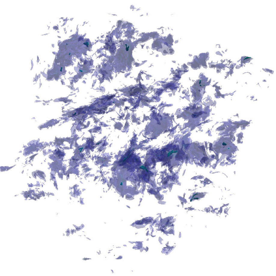
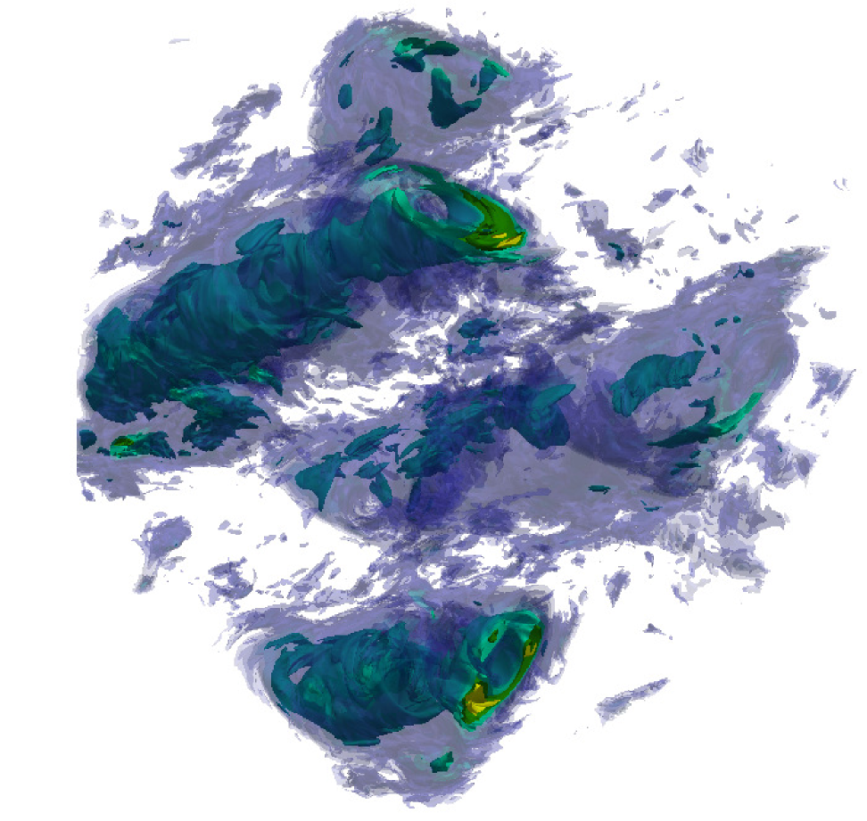
Figure 6: (Color online) Iso-contours of magnitude of velocity fluctuations ($\sqrt{K(t)}$) in run R1 for (left-right) $t/T_{E}^{0}=0,1,11.5$.

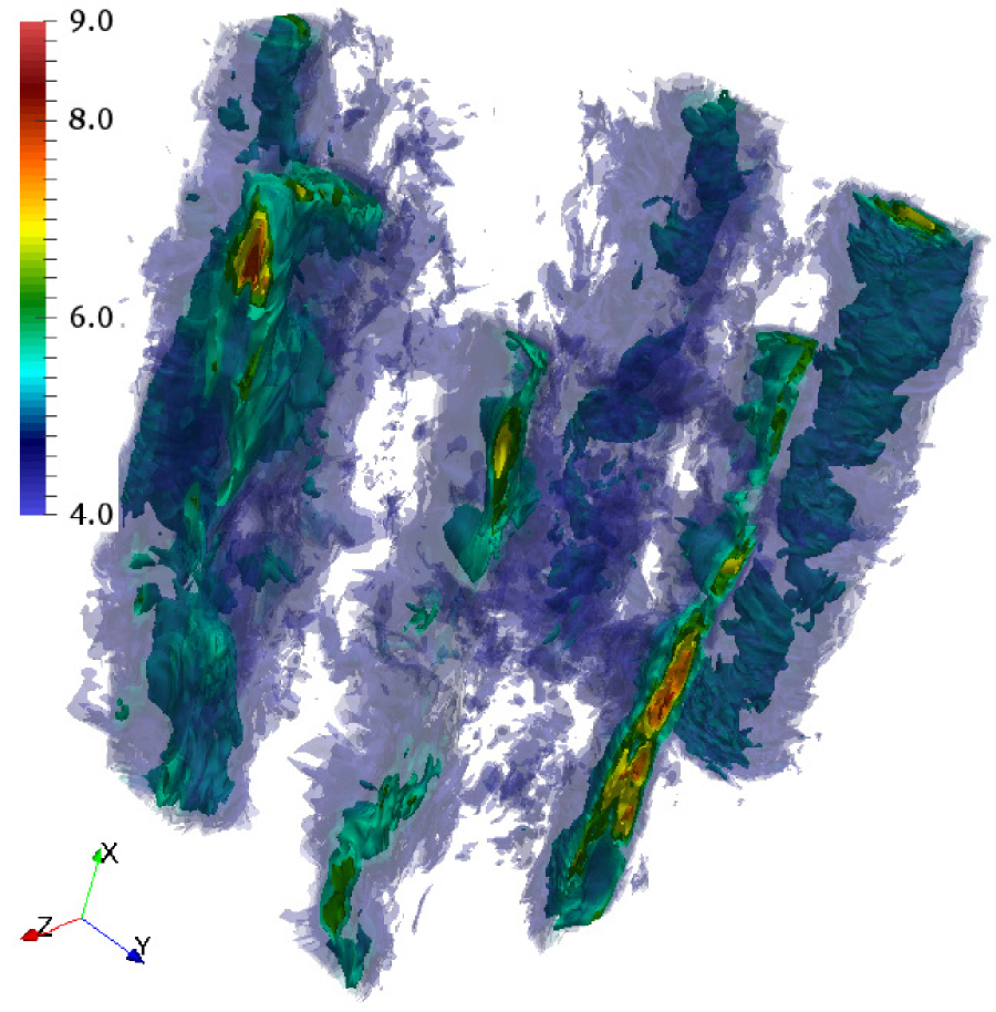
Figure 7: (Color online) Iso-contours of magnitude of velocity fluctuations ($\sqrt{K(t)}$) in run R2 for (left-right) $t/T_{E}^{0}=0,1,6.95$. Note that the iso-contours at $t=0$ for R2 are the same as that for R1 at $t=0$ (left panel in Fig. 6) as both runs start from same initial conditions.

3.3 Large scale structure

Independent of the realizability of the numerical experiments shown here, an important consideration in turbulence subjected to rotation is the robustness and universality of the large scale structures under sudden perturbations of the large scale set-up SM14 . Figures 6 and 7 show the iso-contours of the velocity magnitude at three different time instants in simulations R1 and R2 respectively. For $t\leq 0$, the inverse cascade in the plane normal to the rotation axis manifests itself as columnar structures along the axis of rotation map09 . Shortly after the change in the orientation of the rotation axis at $t=0$, the inverse cascade is suppressed for both runs R1 and R2 but their further evolution differ. In run R1 after a transient, the energy flux becomes positive again at the large scales and diminishes in magnitude at the small scales (Fig. 5). On the other hand, in run R2 the inverse cascade dynamics has insufficient time to recover and the direct cascade is stronger. This can be illustrated by the time evolution of the maximum (negative) amplitude of the flux which is non-monotonous only for run R1 (Fig. 5). The large scale structure evolution can be associated with the life-time of the individual eddies versus the time required for the build-up of the forward cascade. At the low Rossby numbers considered, the time between switching the rotation axis is comparable with the rotation time scale. In such a scenario, the inverse cascade does not have the time to rebuild as evidenced by the lack of large scale structures for $t>0$ in Fig. 7. Thus, the columnar structures characteristic of turbulence subjected to rotation in a fixed direction (Fig. 6) are absent when the orientation of the rotation axis is changed fast enough (Fig. 7). The velocity field structure in the case where the rotation axes is regularly changed resembles that of an isotropic field, a visual proof that the inverse energy cascade is not sustained.

Figure 8: Evolution of energy for simulation R1 for two different cases of large-scale damping. Solid curve corresponds to energy removal for wave number $k\in[0.5,2.5]$, while curve with symbols ($\times$) corresponds to $k\in[0.5,1.5]$. Inset shows late-time evolution of transverse integral length scale $L_{21,1}$ normalized by half the length of the domain ($L_{0}$).

Another question we attempt to address is the robustness of the large scale structures as a function of the energy sink mechanism applied at large scales. In simulations R1 and R2 a hypo-viscous mechanism is used to prevent energy condensation that can occur because of upscale energy transfer owing to finite domain considerations in rotating flows xia11 ; SY93 . It is reasonable to expect that the large scale statistics are influenced by the details of the friction mechanism that is used at the low wave numbers. In order to verify this, we changed the energy removed from the largest scales. For instance, in run R1 we removed energy from different wave number shells at the large scales, thus depleting the system differently. Figure 8 shows two such scenarios where the energy is removed from shells $0.5\leq k\leq 2.5$ and $0.5\leq k\leq 1.5$, respectively. Removing energy from a thinner shell results in a steeper increase in energy initially, but ultimately the energy decreases due to the action of large-scale viscosity cher07 . Eventually the energy for the two large scale friction mechanisms become approximately equal and evolve similarly with time. We have also verified that the large scale structures for these two cases (not shown) are qualitatively the same. The inset of Fig. 8 reports the late time ($t>7.5$) evolution of the transverse integral length scale $L_{22,1}$ defined in terms of the two-point correlation as (with no sum over Greek subscripts)

$$L_{\alpha\alpha,\beta}=\frac{1}{\langle u_{\alpha}^{2}\rangle}\int_{0}^{\infty}\Big{\langle}u_{\alpha}(\mathbf{x})u_{\alpha}(\mathbf{x}+r\mathbf{e}_{\beta})\Big{\rangle}\;,$$ (7)

along the direction of the unit vector $\mathbf{e}_{\beta}$. The integral scales for the case where energy is removed from the thicker shell are smaller than for the case where energy is removed from the thinner shell and are thus contaminated by the periodic boundary conditions to a lesser extent.

4 Conclusions

In this study we have used direct numerical simulations to study the response of rotating turbulence to “precession-like” perturbation. A major emphasis has been to examine the large scale structure and energy transfer characteristics when the orientation of the rotation axis is repeatedly changed.

In the case of uniform solid-body rotation with a fixed rotation direction, the spectral transfer and hence dissipation is greatly reduced by rotation. If the orientation of the rotation axis is changed with a time scale comparable with the rotation time scale, the down scale energy transfer and hence dissipation is shown to increase. After a transient period the kinetic energy reaches a quasi-stationary state as the energy input by forcing is balanced by the dissipation at the small scales. The large scales are devoid of columnar structures typically seen in rotating flows and resemble that of an isotropic state. A quantitative assessment of the degree of isotropization due to the change in the orientation of the rotation axis will require a systematic projection onto the eigenfunctions of the group of rotation and will be reported elsewhere LP05 .

This work is a first step in studying the influence of precession-like perturbation on rotating turbulence. We have neglected the time dependent precession term $d(\mathbf{\Omega}\times\mathbf{r})/dt$ under the assumption that the instantaneous perturbation induced by the sudden change in the rotation axis does not affect the long-time dynamical evolution and/or the evolution of the fluid region close enough to the rotation axis. Using a penalization technique the non-homogeneous precession term $d(\mathbf{\Omega}\times\mathbf{r})/dt$ can be taken into account exactly kai05 . Another potential source of spurious effects is due to periodic boundary conditions, which force the large-scale columns to wrap around the lattice, something that would not be possible in presence of a solid boundary fabien . The robustness of these approximations will be quantified in a study presented elsewhere.

5 Acknowledgments

We acknowledge P. Mininni for useful discussions. Annick Pouquet is thankful to LASP for its hospitality. This work was funded by the European Research Council under the European Community’s Seventh Framework Program, ERC Grant Agreement No. $339032$. We acknowledge the CINECA initiatives INF14_fldturb and IscrC_RotEuler for the availability of high performance computing resources and support.

All authors contributed equally to the paper.

References

- (1) C. Cambon, N. N. Mansour and F. S. Godeferd, J. Fluid Mech. 227, 303 (1997)
- (2) N. N. Mansour, T. Shih and W. C. Reynolds, Phys. Fluids 3, 2421 (1991)
- (3) B. Saint-Michel, B. Dubrulle, L. Marié, F. Ravelet and F. Daviaud, New J. Phys. 16, 063037 (2014)
- (4) S. Thalabard, B. Saint-Michel, E. Herbert, F. Daviaud and B. Dubrulle, New J. Phys. 17, 063006 (2015)
- (5) A. Pouquet and P. D. Mininni, Phil. Trans. R. Soc. A 368, 1635 (2010)
- (6) A. Sen, P. D. Mininni, D. Rosenberg and A. Pouquet, Phys. Rev. E 86, 036319 (2012)
- (7) H. Xia, D. Byrne, G. Falkovich and M. Shats, Nature Phys. 7, 321 (2011)
- (8) S. Kida, J. Fluid Mech. 680, 150 (2011)
- (9) S. Goto, N. Ishii, S. Kida, and M. Nishioka, Phys. Fluids 19, 061705 (2007)
- (10) W. V. R. Malkus, Science 160, 259 (1968)
- (11) S. Goto, A. Matsunaga, M. Fujiwara, M. Nishioka, S. Kida, M. Yamato, M. and S. Tsuda, Phys. Fluids 26, 055107 (2014)
- (12) H. P. Greenspan, The Theory of Rotating Fluids (Cambridge Monographs on Mech. & App. Math., Breukelen Press, 1990)
- (13) C. Nore, J. Léorat, J.-L. Guermond and F. Luddens, J. Phys.: Conf. Series 318, 072034 (2011)
- (14) S. A. Triana, D. S. Zimmerman and D. P. Lathrop, J. Geophys. Res. 117, B04103 (2012)
- (15) B. L. Sawford, Phys. Fluids 3, 1577 (1991)
- (16) O. Zeman, Phys. Fluids 6, 3221 (1994)
- (17) K.R. Sreenivasan, Phys. Fluids 7, 2778 (1995)
- (18) Y. Zhou, Phys. Fluids 7, 2092 (1995)
- (19) P. D. Mininni, D. Rosenberg and A. Pouquet, J. Fluid Mech. 699, 263 (2012)
- (20) A.S. Monin, A.M. Yaglom, Statistical Fluid Mechanics, Vol. 2 (MIT Press, 1975)
- (21) P.D. Mininni, A. Alexakis, A. Pouquet, Phys. Fluids 21(1), 015108 (2009)
- (22) L. M. Smith and V. Yakhot, Phys. Rev. Lett. 71, 352 (1993)
- (23) M. Chertkov, C. Connaughton, I. Kolokolov and V. Lebedev, Phys. Rev. Lett. 99, 084501 (2007)
- (24) L. Biferale and I. Procaccia, Phys. Rep. 414, 43 (2005)
- (25) K. Schneider, Computers & Fluids 34, 1223 (2005)
- (26) F. S. Godeferd and F. Moisy, App. Mech. Rev. 67, 030802 (2015)