Composite pulses for high-fidelity population inversion in optically dense, inhomogeneously broadened atomic ensembles

Abstract

We derive composite pulse sequences that achieve high-fidelity excitation of two-state systems in an optically dense, inhomogeneously broadened ensemble. The composite pulses are resistant to distortions due to the back-action of the medium they propagate in and are able to create high-fidelity inversion to optical depths $\alpha z>10$. They function well with smooth pulse shapes used for coherent control of optical atomic transitions in quantum computation and communication. They are an intermediary solution between single $\pi$-pulse excitation schemes and adiabatic passage schemes, being far more error tolerant than the former but still considerably faster than the latter.

I Introduction

Coherent control methods that achieve the precise manipulation of atomic quantum states play a vital role in quantum information processing and quantum communication. One class of methods that was applied extensively in this field utilizes various forms of adiabatic passage Vitanov et al. (2001); Král et al. (2007). While adiabatic methods possess robust fault tolerance, their slow speed can be a serious disadvantage. Therefore alternative methods were developed using various optimization schemes with the aim of speeding the control process up, but at the same time retaining at least some of the fault tolerance Chen et al. (2010); Ruschhaupt et al. (2012); Torrontegui et al. (2013); Daems et al. (2013); Hegerfeldt (2013). One of these alternative approaches is the method of composite pulses (also called composite pulse sequences) that was originally developed in NMR Levitt (1986); Jones (2003), but has recently found its way into coherent control and quantum information processing Cummins et al. (2003); Roos and Mølmer (2004); Torosov and Vitanov (2011); Torosov et al. (2011); Genov et al. (2011); Kyoseva and Vitanov (2013); Torosov and Vitanov (2014); Torosov et al. (2015); Genov et al. (2014) .

One specific task in quantum information processing is building an optical quantum memory - a device that can store and retrieve the quantum state of a single-photon light pulse Lvovsky et al. (2009). This is an indispensable component of quantum repeaters, devices that allow long-range quantum communication Sangouard et al. (2007, 2011), but of also a number of other quantum technologies Bussières et al. (2013). Memory schemes based on inhomogeneously broadened atomic ensembles (such as rare-earth ion doped optical crystals) and some variant of the photon echo effect have been studied intensively in recent years Tittel et al. (2010); Sangouard et al. (2011). Some of these achieve the rephasing of atomic coherences that is necessary for the echo emission by inverting (a part of) the atomic ensemble with laser pulses Damon et al. (2011); McAuslan et al. (2011); Dajczgewand et al. (2014). The difficulty is that the ensemble must be optically dense to absorb the signal, which means that it will also distort the control pulses that are meant to produce population inversion. Thus inverting an inhomogeneously broadened, optically dense ensemble of atoms is not a simple task, yet it is an important skill to master if these photon-echo type memories are to reach maturity.

Using single Rabi $\pi$-pulses in an optically dense ensemble is problematic because the pulse is quickly rendered ineffective by the medium Ruggiero et al. (2009); Demeter (2013). Control pulses that utilize adiabatic passage are more convenient Zafarullah et al. (2007); Damon et al. (2011); Demeter (2013, 2014), but depending on the maximum pulse amplitude possible (limited for example by the maximum available laser power or the damage threshold of the crystal that hosts the ensemble) they may be too time consuming. The method of composite pulses (CPs) involves constructing complex control pulses for quantum state manipulation from a sequence of simple “elementary” pulses. Free parameters in the construction can be used to obtain fault tolerance with respect to various errors of the constituent pulses, such as frequency offsets or amplitude errors. Even “universal” CPs can be developed that tolerate arbitrary imperfections. The method of CPs has recently been used to develop error tolerant, high-fidelity population inversion schemes using smooth pulse shapes that are encountered in the optical regime Torosov and Vitanov (2011); Torosov et al. (2011); Genov et al. (2014). In terms of speed and error tolerance, CPs can be regarded as a compromise between the single Rabi $\pi$-pulse and adiabatic passage methods.

In this paper we investigate the use of CPs for robust, high fidelity population inversion in inhomogeneously broadened, optically dense atomic ensembles for quantum information processing purposes. Similar to Torosov and Vitanov (2011) we try to perform the inversion using a CP built from a sequence of $N$ monochromatic Rabi $\pi$-pulses with appropriately chosen phases. We seek sets of phases (phase sequences) that allow the CP to invert an extended region within the ensemble (in terms of spectral width and optical depth) despite pulse distortions due to propagation in the medium. The usual approach in deriving CPs assumes that the error that the phase sequence must compensate arises due to some imperfection of the experimental parameters such that it is reproduced for each elementary pulse of the sequence. In our case however, the pulses are distorted while propagating, and they are not all distorted the same way because some pulses excite the atoms while some return them to the ground state.

The paper is divided as follows. In section II we describe the basic physical setting and the equations to be solved. In section III we generalize the method of Torosov and Vitanov (2011) to derive CPs that are resilient with respect to amplitude errors due to the back action of the optically dense medium on the pulses. The key point here is that we allow the amplitude of even and odd numbered pulses of the sequence to change differently. In section IV we derive CPs where amplitude error compensation is combined with a compensation of the atomic resonance frequency offset from the inhomogeneously broadened line center. Finally in section V we present numerical simulations results of the Maxwell-Bloch equations for resonant pulse propagation. We also investigate the applicability of “universal” CPs derived recently in Genov et al. (2014) for high-fidelity inversion in optically dense ensembles.

II Computing propagators in an optically dense medium

The physical setting we consider consists of an inhomogeneously broadened, spatially extended ensemble of two-level atomic systems. The number density $\mathcal{N}$ of the absorbers is uniform in space and the precise resonance frequency of the $j$-th atom is offset by $\Delta_{j}$ from the inhomogeneous line center $\omega_{0}$: $\Delta_{j}=\omega_{j}-\omega_{0}$. The distribution of atomic frequencies $g(\Delta)$ is constant in space and assumed to be sufficiently wide to be taken a constant $g_{0}$ in the spectral region of the laser fields. A one dimensional propagation of CPs is considered along the $z$ direction, where the ensemble is optically dense. At the entry $z=0$, the CP consist of $N=2n+1$ monochromatic pulses tuned to resonance with the atomic line center $\omega_{0}$. Homogeneous decay processes are neglected and the ensemble is assumed to be in the ground state initially.

In this setting, the effect of the CP on the $j$-th atom located at $z_{j}$ is given by the Schrödinger equation for the atomic probability amplitudes $|\psi_{j}\rangle=\alpha_{j}|g\rangle+\beta_{j}|e\rangle$:

$$\partial_{t}\alpha_{j} =\frac{i}{2}\Omega^{*}(z_{j},t)\beta_{j}$$

$$\partial_{t}\beta_{j} =\frac{i}{2}\Omega(z_{j},t)\alpha_{j}-i\Delta_{j}\beta_{j}.$$ (1)

The complex Rabi frequency $\Omega(z_{j},t)=E(z_{j},t)d/\hbar$ characterizes the atom-field coupling [$E(z_{j},t)$ is the slowly varying electric field amplitude at $z_{j}$, $d$ is the dipole matrix element]. In deriving Eq. 1 the central frequency of the absorption line $\omega_{0}$ has been separated and the RWA applied. Provided $\Omega(z_{j},t)$ is known, one can integrate Eq. 1 and describe the effect of the CP on the atoms from the initial time $t_{i}$ until the final $t_{f}$ in terms of the unitary propagator $[\alpha_{j}(t_{f}),\beta_{j}(t_{f})]^{T}=\mathbf{U}_{j}[\alpha_{j}(t_{i}),\beta_{j}(t_{i})]^{T}$, which can be conveniently written in terms of the complex Cayley-Klein parameters as:

$$\mathbf{U}_{j}=\left(\begin{array}[]{cc}a(\Delta_{j},z_{j})&b(\Delta_{j},z_{j})\\ -b(\Delta_{j},z_{j})^{*}&a(\Delta_{j},z_{j})^{*}\end{array}\right).$$

Clearly, the parameters $a(\Delta_{j},z_{j}),b(\Delta_{j},z_{j})$ depend on the location and frequency offset of the atom. The problem is that the field is initially known only at the boundary and has to be computed for $z>0$ from the Maxwell equation for wave propagation. Using the slowly varying envelope approximation this can be written as:

$$\left(\frac{1}{c}\partial_{t}+\partial_{z}\right)\Omega(z,t)=i\frac{\alpha}{\pi g_{0}}\mathcal{P}(z,t)$$ (2)

where $\alpha$ (without any subscript) is the absorption constant $\alpha=\pi g_{0}k\mathcal{N}d^{2}/\varepsilon_{0}\hbar$ and the medium polarization $\mathcal{P}$ that constitutes the back-action of the ensemble on the propagating field is obtained by summing the atomic coherences within an infinitesimally thin region of $z$:

$$\mathcal{P}(z,t)=\sum_{j:z_{j}\in[z-dz,z+dz]}\alpha_{j}^{*}(t)\beta_{j}(t).$$

Equation 2, and consequently the propagator $\mathbf{U}$ can usually be computed only numerically. Furthermore, any result will pertain only to the specific initial state that the ensemble was in before the CP arrived. The choice we made (all atoms in $|g\rangle$) is adapted to quantum memory applications where the absorption of a single- or few-photon signal pulse before the CP amounts to a negligible change in the ensemble initial state when the propagation of a strong classical control field is concerned. In accordance with the requirements encountered in several photon-echo type quantum memory schemes, we seek to establish high-fidelity atomic inversion in an extended region of the ensemble. The figure of merit we use is the error probability that the atoms remain unexcited by the CP: $P_{err}=|\mathbf{U}_{11}|^{2}=|a(\Delta,z)|^{2}$, which is required to be as low as $10^{-2}-10^{-4}$ for high-fidelity quantum information applications. The region must be wide enough around $\Delta=0$ to encompass the spectral width of the absorbed signal and extend to an optical depth of $\alpha z=5-10$. This latter requirement is defined by the fact that the signal, absorbed in the medium as $\sim\exp(-\alpha z)$ is contained in the region $\alpha z<5$ up to an accuracy of $10^{-2}$ and in the region $\alpha z<10$ up to an accuracy of $10^{-4}$.

The standard procedure would now be to build the propagator of the CP from those of the constituent “elementary” pulses and use the free parameters to tune its effect on the atoms. In case the figure of merit used cannot be computed analytically with symbolic values of the parameters, a numerical optimization procedure can also be employed Roos and Mølmer (2004). In our case however, not only is it impossible to obtain analytical formulas for the propagating fields with symbolic parameters, but the numerical solution of 2 is also expensive enough to make the use of numerical optimization practically impossible. Therefore we will use intuition to determine some conditions that we expect will improve the ability of the CP to invert extended regions in the optically dense, inhomogeneously broadened ensemble and then verify a posteriori that this is indeed the case. Similar to Torosov and Vitanov (2011), we will assume that the CP is made up of $N=2n+1$ consecutive Rabi $\pi$-pulses, the only difference between them being an initial phase $\varphi_{k}$. It is also convenient to adapt the “anagram” condition $\varphi_{k}=\varphi_{N+1-k}$ and fix the overall phase of the CP by $\varphi_{1}=\varphi_{N}=0$. Thus the CP is characterized by the composite phase sequence $[0,\varphi_{2},\varphi_{3},\dots,\varphi_{n+1},\varphi_{n},\dots,\varphi_{2},0]$, defined entirely by the set of $n$ phases $\{\varphi_{k}\}_{k=2}^{n+1}$ with which we can optimize the effect of our CP. We assume that the maximum Rabi frequency for all pulses is $\Omega_{0}$ (fixed either by available laser power or the damage threshold of the optical crystal that hosts the impurity ions) and compare the performance of all CPs to that of a single $\pi$-pulse.

III Amplitude error compensated composite pulses

For $\Delta=0$ Eqs. 1 can be solved exactly to obtain the propagator for a single pulse

$$\mathbf{U}_{k}(\varphi_{k})=\left(\begin{array}[]{cc}\cos\frac{\mathcal{A}_{k}}{2}&i\sin\frac{\mathcal{A}_{k}}{2}e^{i\varphi_{k}}\\ i\sin\frac{\mathcal{A}_{k}}{2}e^{-i\varphi_{k}}&\cos\frac{\mathcal{A}_{k}}{2}\end{array}\right)$$ (3)

where the final level of atomic excitation is determined solely by the pulse area $\mathcal{A}=\int\Omega(t)dt$. An elegant approach was developed in Torosov and Vitanov (2011) to derive CPs that are fault tolerant with respect to errors of pulse amplitude based on this fact, which we will adapt to our problem. The matrix 3 was used to build the overall propagator as

$$\mathbf{U}=\mathbf{U}_{N}(0)\mathbf{U}_{N-1}(\varphi_{2})\dots\mathbf{U}_{3}(\varphi_{3})\mathbf{U}_{2}(\varphi_{2})\mathbf{U}_{1}(0)$$ (4)

and, assuming that the amplitude of the constituent pulses was not perfect, $\mathcal{A}_{k}=\pi+\varepsilon$ was inserted for the imperfect pulse area. Then $a(\varepsilon)|_{\varepsilon=0}=0$ and various derivatives $\partial_{\varepsilon}^{l}a(\varepsilon)$ were nullified with appropriate choices of $\{\varphi_{k}\}$ to obtain CPs with considerable robustness against amplitude errors, having $P_{err}=\mathcal{O}(\varepsilon^{2N})$. (Since all even order derivatives disappear due to the anagram relation $\varphi_{k}=\varphi_{N+1-k}$, only odd order derivatives pose constraints for the phases.) All of the elementary pulses were identical in this approach (the error is duplicated identically for each one) and the result valid for arbitrary pulse shapes.

Fault tolerance with respect to amplitude errors seems useful also when trying to invert atoms in an optically dense sample. It follows from the famed area theorem McCall and Hahn (1967, 1969) that for a single pulse, $\mathcal{A}=\pi$ is an unstable fixed point of the area equation, so any error will increase during propagation. Furthermore, even though a single perfect $\pi$-pulse should retain its area, due to energy loss it reshapes, gradually becoming longer - which means that its area will eventually start decreasing during the finite time interval allocated for the control. However, inserting the amplitude error compensated CPs of Torosov and Vitanov (2011) into the propagation equations shows that they do not perform better than single $\pi$-pulses at all. The results are shown in Fig. 1 a) and b) where the error contours $P_{err}=10^{-2}$ and $P_{err}=10^{-4}$ are plotted on the $\alpha z-\Delta$ plane (i.e. the boundary of the domain around $\Delta=0,z=0$ within which $P_{err}\leq 10^{-2},10^{-4}$). The data for the plot was obtained by computing $\mathbf{U}$ for a single incident $\cos^{2}$ shaped $\pi$-pulse, the amplitude error compensated $N=3$ CP defined by $\{\varphi_{2}=2\pi/3\}$ and the $N=5$ CP with $\{\varphi_{2}=2\pi/5,\varphi_{3}=4\pi/5\}$ Torosov and Vitanov (2011). It is evident that while the single pulse can only produce high fidelity population inversion in an extremely limited domain of the ensemble, the $N=3$ and $N=5$ amplitude error compensated CPs are no better.

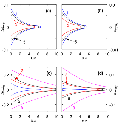
Figure 1: Contour lines of the error probability $P_{err}=|a(\Delta,z)|^{2}$ for amplitude error compensated CPs of Torosov and Vitanov (2011) [a) and b)] and the alternating amplitude error compensated CPs [ c) and d)] on the $\alpha z-\Delta$ parameter plane. a) $P_{err}=10^{-2}$ and b) $P_{err}=10^{-4}$ for a single pulse (blue line), the $N=3$ CP defined by $\{\varphi_{2}=2\pi/3\}$ (red line) and the $N=5$ CP with $\{\varphi_{2}=2\pi/5,\varphi_{3}=4\pi/5\}$ (black line). c) $P_{err}=10^{-2}$ and d) $P_{err}=10^{-4}$ for a single pulse (blue line), the $N=3$ CP designated $U3a$ and defined by $\{\varphi_{2}=\pi/3\}$ (red line), the $N=5$ CP $U5a_{2}:\{\varphi_{2}=\pi/5,\varphi_{3}=8\pi/5\}$ (black line) and the $N=9$ CP $U9a_{8}:\{\varphi_{2}=0.2708\pi,\varphi_{3}=1.0829\pi,\varphi_{4}=0.5898\pi,\varphi_{5}=4\pi/9\}$ (magenta line). Note that the scale on the $z$ axis is the same for all plots, but the scale on the $\Delta$ axis varies. The lines are tagged by $N$ on each subfigure. The first three phases for the 9 pulse sequence are approximate values.

Now it also follows from the area theorem that for a pulse traveling in an inverted medium, the stability properties are reversed: $\mathcal{A}=\pi$ is the stable and $\mathcal{A}=2\pi$ is the unstable solution. Thus the area equation suggests the amplitude error that develops during propagation is not the same for all pulses, so assuming them to be identical is not justified in our case. Indeed it is intuitively clear that a pulse that must excite the atoms of the ensemble will be affected differently during propagation than one that returns them to the ground state. We thus write the error that we seek tolerance against in the following form:

$$\mathcal{A}_{k}=\pi+(-1)^{k}\varepsilon.$$ (5)

This is perhaps the simplest expression that, without introducing new parameters, allows us to differentiate between odd numbered pulses of the composite sequence (i.e. those that are to excite the atoms) and even numbered ones (those which are to return them to the ground state). We will refer to this ansatz as alternating amplitude error. Inserting 5 into Eq. 3, composing the overall propagator 4 and using the constraints $\partial_{\varepsilon}^{l}a(\varepsilon)=0$ for various sets of derivatives, we can derive CPs that are fault tolerant with respect to alternating amplitude errors. For $N=3$, the simplest case, the condition $\partial_{\varepsilon}a=0$ gives $\cos\varphi_{2}=1/2$ which is solved by $\varphi_{2}=\pi/3$, defining the CP designated by $U3a$. Another example is the $N=5$ case where the conditions $\partial_{\varepsilon}a=0$ and $\partial_{\varepsilon}^{3}a=0$ eventually yield $4\cos\varphi_{2}+2\cos(2\varphi_{2}-\varphi_{3})-2\cos\varphi_{3}=1$ and $\cos(\varphi_{2}-\varphi_{3})-\cos(2\varphi_{2}-\varphi_{3})=1/2$. ($\partial_{\varepsilon}^{2}a=0$ and $\partial_{\varepsilon}^{4}a=0$ are satisfied automatically.) Solving these equations we obtain the sequences $U5a_{1}:\{\varphi_{2}=3\pi/5,\varphi_{3}=4\pi/5\}$ and $U5a_{2}:\{\varphi_{2}=\pi/5,\varphi_{3}=8\pi/5\}$. (The designation $U5a_{j}$ means that it is the $j$-th phase sequence with $N=5$ and alternating amplitude error compensation.) Since all even order derivatives of $a(\varepsilon)$ disappear due to the anagram relation, for an $N$ pulse CP where we have $n=(N-1)/2$ phases to nullify derivatives, the first nonzero derivative will be the $N$-th order one, so $P_{err}=\mathcal{O}(\varepsilon^{2N})$. The procedure can be continued to higher orders, but of course the resulting trigonometric equations will be progressively more difficult to solve. Up to $N=9$ we have found, for the $N=2n+1$ phase sequence, $2^{n-1}$ solutions. All the phases obtained are tabulated in table 1 of the appendix.

Inserting the CPs derived in this manner in Eq. 2 we can verify that they are indeed more fault tolerant with respect to propagation induced distortions than a single $\pi$-pulse. Figure 1 c) and d) show the $P_{err}=10^{-2}$ and $P_{err}=10^{-4}$ contours for several CPs together with the single pulse case. It can be seen that increasing $N$ leads to the expansion of the high-fidelity population transfer domain. For $N=9$ the $P_{err}=10^{-4}$ domain already extends past $\alpha z=10$ and it is also about an order of magnitude wider in $\Delta$ than for the single pulse case. The performance of a CP can only be evaluated by computing the propagating fields numerically - the CPs depicted are the ones that perform best for each $N$. An $N=7$ sequence was omitted in the figure because the best 7 pulse CP was only slightly better than the $N=5$ one depicted. Note that if the sequence $\{\varphi_{k}\}$ is a valid solution, then so is $\{-\varphi_{k}\}$ and thus $\{2\pi-\varphi_{k}\}$ - we consider these sequences to be identical (they are not listed in table 1). The figures were produced by using $\cos^{2}$ shaped pulses - they are convenient to use because they become exactly zero at a finite time point.

IV Frequency offset and amplitude error compensation

Composite pulses with alternating amplitude error compensation allow the $P_{err}<10^{-4}$ region to reach $\alpha z>10$, which is perfectly sufficient. The region is still fairly narrow with respect to the frequency offset $\Delta$, so we now seek to derive CPs with combined error compensation of alternating amplitude error and frequency offset. However, when $\Delta\neq 0$ the Cayley-Klein parameters depend on the shape of the pulse envelope, so we turn to pulse shapes for which Eqs. 1 are analytically solvable.

IV.1 Hyperbolic-secant pulse

First we use the following solution for the Rosen-Zener model Rosen and Zener (1932); Torosov and Vitanov (2011), for which $\Omega(t)=\Omega_{0}\mathrm{sech}(t/T)$ and the frequency offset (detuning) is constant. The Cayley-Klein parameters for the $k$-th pulse with phase $\varphi_{k}$ are:

$$a_{k} =\frac{\Gamma\left(\frac{1}{2}+iq\right)^{2}}{\Gamma\left(\frac{1}{2}+iq-p\right)\Gamma\left(\frac{1}{2}+iq+p\right)}$$

$$b_{k} =i\frac{\sin\pi p}{\cosh\pi q}e^{i\varphi_{k}}$$ (6)

where $p=\Omega_{0}T/2$ and $q=\Delta T/2$. Clearly, for $\Omega_{0}T=1$ we have the $\pi$-pulse case, $b=ie^{i\varphi},a=0$. We insert the alternating amplitude error ansatz for the $m$-th pulse as $\Omega_{0}T=1+(-1)^{m}\varepsilon$ in Eqs. 6 and create the CP propagator via 4 as before. We then seek phase sequences where various derivatives of $a(\varepsilon,\Delta)$ are zero at $\varepsilon=0,\Delta=0$.

For $N=3$ we have two equations from the first derivatives $\partial_{\Delta}a=0$ and $\partial_{\varepsilon}a=0$, but they both yield the same constraint for $\varphi_{2}$: $\cos\varphi_{2}=1/2$ which is satisfied by $\varphi_{2}=\pi/3$. The CP designated $U3c$ and defined by $\{\varphi_{2}=\pi/3\}$ has been derived in Torosov and Vitanov (2011) as a detuning compensated CP, and the previous section of the present paper as the alternating amplitude error compensated CP $U3a$ for arbitrary pulse shapes. We now see that for hyperbolic-secant pulse shape it is a CP with combined frequency offset / alternating amplitude error compensation. The order of the error for this sequence is $P_{err}=\mathcal{O}(\Delta^{4}),\mathcal{O}(\varepsilon^{4})$.

For $N=5$ the equations $\partial_{\Delta}a=0$ and $\partial_{\varepsilon}a=0$ again both yield the same constraint for the phases:

$$1-2\cos(\varphi_{2}-\varphi_{3})+2\cos(2\varphi_{2}-\varphi_{3})=0.$$ (7)

Computing the second derivatives shows that the conditions obtained from the equations $\partial_{\Delta}^{2}a=0$ and $\partial_{\varepsilon}\partial_{\Delta}a=0$ are also equivalent:

$$1+2\cos(\varphi_{2}-\varphi_{3})+2\cos(2\varphi_{2}-\varphi_{3})=0.$$ (8)

($\partial_{\varepsilon}^{2}a=0$ is automatically fulfilled). These two conditions are then satisfied by two phase sequences: $U5c_{1}:\{\varphi_{2}=5\pi/6,\varphi_{3}=\pi/3\}$ and $U5c_{2}:\{\varphi_{2}=\pi/6,\varphi_{3}=5\pi/3\}$. (The designation of the form $U5c_{i}$ means that it is the $i$-th CP with $N=5$ and combined error compensation.) $P_{err}\sim\mathcal{O}(\Delta^{6}),\mathcal{O}(\varepsilon^{6})$ for these sequences.

For $N=7$, $\partial_{\Delta}a=0$ and $\partial_{\varepsilon}a=0$ again yield a single constraint

$$1-2\cos(\varphi_{3}-\varphi_{4})+2\cos(\varphi_{2}-2\varphi_{3}+\varphi_{4})\\ -2\cos(2\varphi_{2}-2\varphi_{3}+\varphi_{4})=0,$$ (9)

while $\partial_{\Delta}^{2}a=0$ and $\partial_{\varepsilon}\partial_{\Delta}a=0$ both reduce to:

$$1+2\cos(\varphi_{3}-\varphi_{4})+2\cos(\varphi_{2}-2\varphi_{3}+\varphi_{4})\\ +2\cos(2\varphi_{2}-2\varphi_{3}+\varphi_{4})=0.$$ (10)

Computing all third order derivatives we find that from $\partial_{\Delta}^{3}a=0$, $\partial_{\varepsilon}\partial_{\Delta}^{2}a=0$, $\partial_{\varepsilon}^{2}\partial_{\Delta}a=0$ and $\partial_{\varepsilon}^{3}a=0$ we obtain only one more constraint for the phases. Any one of these four equations can be used together with Eqs. 9 and 10 to obtain the same phase sequences because any of the third order derivatives can be expressed as a linear combination of another one, (say $\partial_{\Delta}^{3}a$) and Eqs. 9, 10. Thus for $N=7$ we can nullify all derivatives up to third order using six phase sequences tabulated in table 2 of the appendix as $U7c_{1}-U7c_{6}$. These sequences yield CPs with $P_{err}=\mathcal{O}(\Delta^{8}),\mathcal{O}(\varepsilon^{8})$.

Finally we have considered the $N=9$ case. Similar to the $N=3,5$ and $N=7$ cases, we found that all the equations from a given order of derivatives essentially yield only one additional independent constraint for the phases. Thus solving four trigonometric equations gives us phase sequences where all derivatives of $a(\varepsilon,\Delta)$ will be nullified up to fourth order, yielding CPs with $P_{err}\sim\mathcal{O}(\varepsilon^{10}),\mathcal{O}(\Delta^{10})$. The twelve phase sequences obtained are tabulated in the appendix in table 2 for reference, designated $U9c_{1}-U9c_{12}$.

It is remarkable, that for hyperbolic-secant pulses, we have been able to nullify all the derivatives up to $n$-th order with $n$ phase parameters all the way up to $n=4$ (i.e. $N=9$). For $N=11$ and higher the expressions for the derivatives become intractable, so it is unclear whether this trend continues. However it must be noted that nullifying so many derivatives with so few parameters is possible because of the symmetries inherent in the alternating amplitude error ansatz 5 and the anagram relation together. A less symmetric amplitude error ansatz can easily lead to constraints that can not all be satisfied simultaneously. Relaxing the anagram relation allows more phase parameters for the same pulse number $N$, but more independent constraints per level of derivatives - overall there is no gain.

IV.2 Comments on other pulse shapes

Two important questions immediately arise. First, do the CP-s derived in the previous subsection actually show improved performance when propagating in the ensemble and how does this performance increase with the number of pulses $N$? Second, are the results applicable to other pulse shapes? The second question is important because hyperbolic-secant pulses fall off very slowly, so, with the time required for the operation being an important factor, more compact pulses such as Gaussian or $\cos^{2}$ pulse shapes are preferable.

To gain insight into the second question, we have repeated the derivation outlined above for square pulses. While not very relevant for short pulses in the optical domain, they too allow analytic solution of Eqs. 1. We have found, that up to $N=7$ we obtain precisely the same constraints and solutions for the phases as for hyperbolic-secant pulses. However, for $N=9$ the square-pulse case deviates. The equations obtained from the fourth order derivatives can no longer be reduced to a single constraint. Thus the four phases we have for $N=9$ are no longer sufficient to nullify all fourth order derivatives for square pulses.

More insight can be gained by noting that the 3 and 5 pulse CPs have been derived before. First, $U3a/U3c$, has been derived in Torosov and Vitanov (2011) as a detuning compensated sequence and it has also been stated that up to $N=5$ detuning compensated CPs are independent of the pulse shape, provided that it is symmetric in time: $\Omega(t)=\Omega(-t)$. Next, $U5c_{1}$ has also been found in Torosov and Vitanov (2011) as a CP with simultaneous compensation of amplitude error and detuning. Finally, $U5c_{1}$ and $U5c_{2}$ have been derived in Genov et al. (2014) (denoted $U5a$ and $U5b$ there) as “universal” CPs, sequences that compensate pulse errors to first order regardless of their nature (imperfect pulse shape, amplitude, detuning, chirp, etc. - provided that it is exactly reproduced for all of the pulses).

Repeating the derivation in subsection IV.1 using uniform amplitude error $\Omega_{0}T=1+\varepsilon$, we find that for $N=5$, $\partial_{\Delta}a=0$ yields condition 7, while $\partial_{\varepsilon}a=0$ reduces to condition 8. Of the second order derivatives, $\partial_{\Delta}^{2}a=0$ yields constraint 8 and $\partial_{\Delta}\partial_{\varepsilon}a=0$ yields constraint 7. So for the uniform amplitude error considered in Torosov and Vitanov (2011) we need two phases to nullify both first order derivatives - but then the second order ones are simultaneously nullified as well. Thus $U5c_{1}$ and $U5c_{2}$ are in fact CPs that compensate both frequency offset (detuning) and uniform amplitude error / alternating amplitude error simultaneously up to second order. All these point to $U5c_{1}$ and $U5c_{2}$ being combined alternating amplitude error / frequency offset compensated sequences for arbitrary (symmetric) pulse shapes.

V Simulation results for CP propagation

To verify that the CPs derived in section IV.1 do perform better at inverting an optically dense ensemble, we have computed their propagation for three different smooth pulse envelopes using Eq. 2 - hyperbolic-secant: $\Omega_{s}(t)=\Omega_{0}\mathrm{sech}(t/T_{s})$, Gaussian: $\Omega_{g}(t)=\Omega_{0}\exp(-t^{2}/2T_{g}^{2})$ and $\cos^{2}$: $\Omega_{c}(t)=\Omega_{0}\cos^{2}(t\pi/2T_{c})$. The same peak pulse amplitude $\Omega_{0}$ was used in all three cases and the time constants were adjusted so that pulse areas were $\pi$: $T_{s}=1$, $T_{g}=\sqrt{\pi/2}$ and $T_{c}=\pi$. Using the field $\Omega(z,t)$ obtained from the simulation, $\mathbf{U}(\Delta,z)$ was computed and the error contours $P_{err}=|a(\Delta,z)|^{2}$ plotted on the $\alpha z-\Delta$ plane.

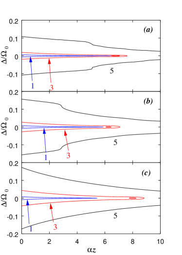
Figure 2: Contour lines of $P_{err}=10^{-4}$ on the ${\alpha}z\mathrm{-}\Delta$ plane for a single $\pi$-pulse (line 1), the $N=3$ CP $U3c:\{\varphi_{2}=\pi/3\}$ (line 3) and the $N=5$ CP $U5c_{2}:\{\varphi_{2}=\pi/6,\varphi_{3}=5\pi/3\}$ (line 5) in case of a) hyperbolic-secant pulses, b) Gaussian pulses and c) $\cos^{2}$ shaped pulses.

Figure 2 shows the $P_{err}=10^{-4}$ contours for a) hyperbolic-secant, b) Gaussian and c) $\cos^{2}$ pulse shapes. The lines tagged by 1, 3 and 5 belong to a single $\pi$-pulse, the $U3c$ and the $U5c_{2}$ sequences respectively on all three subfigures. One can see that for all three pulse shapes the $U3c$ and $U5c_{2}$ sequences show greatly improved performance over the single $\pi$-pulse. The spectral width of the high-fidelity population transfer region for the $U5c_{2}$ CP is about 20 times wider at $\alpha z=0$ and about 120 times wider at $\alpha z=5$ for all three pulse shapes. This corroborates the conjecture that these sequences are universal and should work for arbitrary symmetric pulse shapes. It is important to note that the two $N=5$ CPs do not perform equally well. $U5c_{1}$ (not depicted here) is considerably better than the $U3c$ sequence, but is systematically inferior to the $U5c_{2}$ one. This is because after all second order derivatives are nullified, the (nonzero) values of the third order derivatives will matter most. For the hyperbolic-secant pulse where these derivatives can be evaluated, we found the four third order derivatives to be about an order of magnitude smaller for the $U5c_{2}$ sequence.

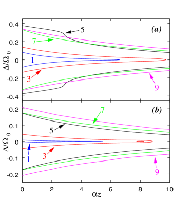
Figure 3: Contour lines of a) $P_{err}=10^{-2}$ and b) $P_{err}=10^{-4}$ on the ${\alpha}z\mathrm{-}\Delta$ plane. The lines tagged by 1, 3, 5, 7 and 9 correspond to the single-pulse case and to the CPs $U3c:\{\varphi_{2}=\pi/3\}$, $U5c_{2}:\{\varphi_{2}=\pi/6,\varphi_{3}=5\pi/3\}$, $U7c_{1}:\{\varphi_{2}=-0.647\pi,\varphi_{3}=\pi/3,\varphi_{4}=0.647\pi\}$ and $U9c_{1}:\{\varphi_{2}=0.025\pi,\varphi_{3}=0.847\pi,\varphi_{4}=0.670\pi,\varphi_{5}=1.299\pi\}$ respectively. Phases in fractional form are exact values while phases in decimal form are approximate.

Because the $\cos^{2}$ pulses are the most compact of the above three, (they become exactly zero at finite $t$), this is the pulse shape we have used for investigating longer sequences. Figure 3 shows the $P_{err}=10^{-2}$ and the $P_{err}=10^{-4}$ contours for several CPs up to $N=9$ on the $\alpha z-\Delta$ plane. Evidently the performance does improve with $N$, but the improvement slows considerably after $N=5$. This however is not surprising, as the phases were derived using a series expansion. One can also see that for lower fidelity and optical depth, $U5c_{2}$ beats even the 7 and 9 pulse CPs depicted. Note that we have plotted, out of the six CPs designated $U7c_{1}-U7c_{6}$ and of the 12 designated $U9c_{1}-U9c_{12}$, the ones that show the best performance. It is not strictly true that each $N=9$ CP is better than any $N=7$ CP. This effect is probably due to the values of higher order derivatives that are not nullified as we have seen for $U5c_{1}$ and $U5c_{2}$. Overall, even though the duration of a $N=9$ pulse CP is considerably shorter than pulses that would achieve the population transfer via AP, the best tradeoff seems to be $N=5$, where the $P_{err}<10^{-4}$ region already reaches $\alpha z=10$. Note also that CPs with combined error compensation are superior to CPs with solely alternating amplitude error compensation. Comparing the lines on Fig. 1 d) and 3 c) (both represent $\cos^{2}$ shaped pulses) one can see that the $N=5$ CP with combined error compensation is better than the $N=9$ CP with only amplitude error compensation.

As the sequences $U5c_{1}$ and $U5c_{2}$ derived here have also turned up as “universal composite pulses” in a very different setting in Genov et al. (2014), we carried out a detailed investigation of all the CPs derived there as they propagate in the optically dense medium. The derivation there did not assume any constraint on the nature of the compensated imperfection or the shape of the pulse (hence the term “universal”), only that it is exactly the same for all elementary pulses. Phase sequences were derived for $N=5,7$ and $9$ pulse CPs which compensate the errors up to second order, $N=13$ CPs that compensate them to fourth order and $N=25$ CPs that do so to eighth order.

We have substituted the phases tabulated in table I. of Genov et al. (2014) for the CPs $U7a$, $U7b$, $U9a$ and $U9b$ into the constraints derived in section IV.1 for hyperbolic-secant pulses. We found the sequences to satisfy the constraints derived from the first and second order derivatives, but not the third order ones. Correspondingly, computing their propagation using Eqs. 2 we found that their performance is practically the same as that of the $U5c_{2}$ CP (the shortest one that allows combined error compensation to second order). By comparison, the $U7c_{1}$ and $U9c_{1}$ CPs derived in the present work did function better than $U5c_{2}$, even if the increase in performance was not as prominent as during the $N=3$ to $N=5$ step.

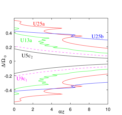
Figure 4: Contour lines of $P_{err}=10^{-4}$ on the ${\alpha}z\mathrm{-}\Delta$ plane for some CPs derived in Genov et al. (2014). The lines tagged by $U5c_{2}$ (black) and $U9c_{1}$ (magenta - dashed line) correspond to CPs derived in this paper (as well).

While we have not been able to derive phases for combined error compensation CPs higher than $N=9$, it is still interesting to check the performance of the $N=13$ and $N=25$ “universal” sequences. Figure 4 shows the error contours that mark the boundary of high-fidelity inversion for several CPs. For $N=13$, we have plotted $U13a$ which is clearly better, but for $N=25$ the two CPs $U25a$ and $U25b$ are both shown - the former is better for smaller optical depths while the latter is superior for larger ones. For a comparison, the $U9c_{1}$ CP derived here and the $U5c_{2}$ CP derived in both papers are also shown. Clearly, there is a considerable increase in performance with $N$ which is intriguing because it suggests that CPs with $N>9$ and combined alternating amplitude / frequency offset error compensation can be derived to achieve still higher performance in inverting an optically dense ensemble. One must keep in mind however, that very long sequences (such as $N=25$) are not practical because the time required already allows adiabatic passage schemes to function better.

Another problem must be considered when employing CPs for inverting optically dense ensembles, namely the time window in which the amplitude of the pulse sequence is appreciably different from zero at a given optical depth. A single $\pi$-pulse increases its temporal length as it propagates, developing a long “tail” that can overlap any signal echos that are to be retrieved from the ensemble Ruggiero et al. (2009), making its application impractical. A similar effect can be observed with some of the CPs studied in this paper. For some phase sequences a long oscillatory tail develops as the CP propagates, increasing the time window where the control field is non-negligible. This does not affect all sequences equally, some CPs are much less affected than others. It is a property that has to be investigated for each sequence separately when considering its application in photon-echo quantum memory schemes.

Finally, some comments on the validity of the two-level model without relaxation are in order. To achieve high-fidelity quantum state control, the entire manipulation process has to be concluded in a time $T_{CP}$ much less than the lifetime $T_{1}$ of the atomic excited state (or the coherence lifetime $T_{2}$ if that is shorter). Given the requirement $P_{err}<10^{-2},10^{-4}$, we can readily estimate the time available as $T_{CP}<P_{err}T_{1}$. (A more precise calculation using a master equation for the two-state system shows that this is in fact an overestimation, but it is very useful for order of magnitude considerations.) Conversely, if the interaction time is shorter than this limit, relaxation can be neglected for our purposes. For a number of rare-earth ions such as erbium, thulium, europium or terbium that can be described as two-state systems in optical crystals under certain conditions, excited state lifetimes in the range of 1-10 ms were measured Thiel et al. (2011). The time available for the manipulation in these cases is then $10-100\mu s$ (for $P_{err}=10^{-2}$) and $0.1-1\mu s$ (for $P_{err}=10^{-4}$). Of course, for longer composite sequences this means shorter elementary pulses, so very long sequences are inconvenient.

VI Summary and Outlook

In this paper, we have investigated the use of composite pulses for the high-fidelity inversion of two-level systems in an optically dense, inhomogeneously broadened ensemble. Such ensembles, found for example in rare-earth doped optical crystals, have important applications in quantum communication and quantum computing , e.g. as a medium for realizing photon-echo based optical quantum memories. High-fidelity inversion in optically dense media is problematic because they distort the pulses as they propagate.

We have introduced the concept of alternating amplitude error (amplitude error that is of opposite sign for even and odd numbered pulses of the sequence) and have derived phase sequences that grant the CP robustness with respect to it. We have shown that these CPs are then able to invert the atoms of the ensemble to a greater optical depth than single $\pi$-pulses. When alternating amplitude error compensation is combined with frequency offset compensation, we obtain CPs that are even more effective. Using CPs made up of of as few as five pulses, the region of high-fidelity inversion can easily reach an optical depth of $\alpha z=10$ and be over two orders of magnitude wider in spectral width than the inversion obtained using a single $\pi$-pulse. The phase sequences were derived using series expansions of various analytically solvable models for two-level atomic excitation. Their performance in creating high-fidelity inversion within the ensemble was then verified by numerical simulation of the Maxwell-Bloch equations for pulse propagation. Finally, we have also verified that some of the universal composite pulses derived in Genov et al. (2014) are also effective at creating high-fidelity inversion in optically dense ensembles.

Overall, some of the CPs derived demonstrate great potential for inverting optically dense ensembles - they are much more robust than single monochromatic $\pi$-pulses, but can be considerably faster than adiabatic passage methods. Furthermore, one can possibly refine further the phase sequences using numerical optimization schemes. Numerical schemes that need to solve the Maxwell-Bloch equations at each step are far too expensive computationally to perform an optimization from the start. They may, however be suitable to obtain an even higher performance by using one of the sets of phases derived in this paper as a starting point and executing the optimization scheme only for a very limited number of steps.

Appendix A Complete list of phases

Below is a list of phases for the alternating amplitude error compensated CPs derived in section III and the combined error compensation CPs from section IV.

designation	$\varphi_{2}$	$\varphi_{3}$	$\varphi_{4}$	$\varphi_{5}$
$U3a$	1/3
$U5a_{1}$	3/5	4/5
$U5a_{2}$	1/5	8/5
$U7a_{1}$	1/7	10/7	13/7
$U7a_{2}$	0.230	1.230	1
$U7a_{3}$	3/7	2/7	11/7
$U7a_{4}$	5/7	8/7	9/7
$U9a_{1}$	1/9	4/3	5/3	10/9
$U9a_{2}$	1/3	0	1/3	2/3
$U9a_{3}$	1/3	0	5/3	0
$U9a_{4}$	5/9	2/3	1/3	14/9
$U9a_{5}$	7/9	4/3	5/3	16/9
$U9a_{6}$	0.145	1.280	0.024	2/9
$U9a_{7}$	0.199	1.803	1.160	8/9
$U9a_{8}$	0.271	1.083	0.590	4/9

Table 1: List of phases given as multiples of $\pi$ for alternating error compensated CPs derived in section III. Phases in fractional form are exact values while phases in decimal form are approximate.

designation	$\varphi_{2}$	$\varphi_{3}$	$\varphi_{4}$	$\varphi_{5}$
$U3c$	1/3
$U5c_{1}$	5/6	1/3
$U5c_{2}$	1/6	5/3
$U7c_{1}$	-0.647	1/3	0.647
$U7c_{2}$	-0.176	1/3	0.176
$U7c_{3}$	0.425	1/3	-0.425
$U7c_{4}$	0.536	1/3	-0.536
$U7c_{5}$	0.193	1.386	1.245
$U7c_{6}$	0.955	0.911	1.533
$U9c_{1}$	0.025	0.847	0.670	1.299
$U9c_{2}$	0.057	1.30	1.911	0.095
$U9c_{3}$	0.126	1.454	1.916	1.983
$U9c_{4}$	0.128	1.458	1.789	1.724
$U9c_{5}$	0.431	1.189	0.572	0.385
$U9c_{6}$	0.500	0.606	0.304	1.601
$U9c_{7}$	0.526	0.609	0.294	1.595
$U9c_{8}$	0.721	0.254	0.878	1.925
$U9c_{9}$	0.731	0.261	0.791	1.721
$U9c_{10}$	0.782	1.474	0.530	0.212
$U9c_{11}$	0.808	0.779	1.751	0.084
$U9c_{12}$	0.866	0.570	0.814	1.585

Table 2: List of phases given as multiples of $\pi$ for combined error compensated CPs derived in section IV.1. Phases in fractional form are exact values while phases in decimal form are approximate.

References

- Vitanov et al. (2001) N. V. Vitanov, T. Halfmann, B. W. Shore, and K. Bergmann, Annual Review of Physical Chemistry 52, 763 (2001).
- Král et al. (2007) P. Král, I. Thanopulos, and M. Shapiro, Reviews of Modern Physics 79, 53 (2007).
- Chen et al. (2010) X. Chen, I. Lizuain, A. Ruschhaupt, D. Guéry-Odelin, and J. Muga, Physical Review Letters 105, 123003 (2010).
- Ruschhaupt et al. (2012) A. Ruschhaupt, X. Chen, D. Alonso, and J. Muga, New Journal of Physics 14, 093040 (2012).
- Torrontegui et al. (2013) E. Torrontegui, S. Ibáñez, S. Martínez-Garaot, M. Modugno, A. del Campo, D. Guéry-Odelin, A. Ruschhaupt, X. Chen, and J. G. Muga, Adv. At. Mol. Opt. Phys 62, 117 (2013).
- Daems et al. (2013) D. Daems, A. Ruschhaupt, D. Sugny, and S. Guérin, Physical Review Letters 111, 050404 (2013).
- Hegerfeldt (2013) G. C. Hegerfeldt, Physical Review Letters 111, 260501 (2013).
- Levitt (1986) M. H. Levitt, Progress in Nuclear Magnetic Resonance Spectroscopy 18, 61 (1986).
- Jones (2003) J. A. Jones, Philosophical Transactions of the Royal Society of London A: Mathematical, Physical and Engineering Sciences 361, 1429 (2003).
- Cummins et al. (2003) H. K. Cummins, G. Llewellyn, and J. A. Jones, Physical Review A 67, 042308 (2003).
- Roos and Mølmer (2004) I. Roos and K. Mølmer, Physical Review A 69, 022321 (2004).
- Torosov and Vitanov (2011) B. T. Torosov and N. V. Vitanov, Physical Review A 83, 053420 (2011).
- Torosov et al. (2011) B. T. Torosov, S. Guérin, and N. V. Vitanov, Physical Review Letters 106, 233001 (2011).
- Genov et al. (2011) G. Genov, B. Torosov, and N. Vitanov, Physical Review A 84, 063413 (2011).
- Kyoseva and Vitanov (2013) E. Kyoseva and N. V. Vitanov, Physical Review A 88, 063410 (2013).
- Torosov and Vitanov (2014) B. T. Torosov and N. V. Vitanov, Physical Review A 90, 012341 (2014).
- Torosov et al. (2015) B. Torosov, E. Kyoseva, and N. Vitanov, Physical Review A 92, 033406 (2015).
- Genov et al. (2014) G. T. Genov, D. Schraft, T. Halfmann, and N. V. Vitanov, Physical Review Letters 113, 043001 (2014).
- Lvovsky et al. (2009) A. I. Lvovsky, B. C. Sanders, and W. Tittel, Nature Photonics 3, 706 (2009).
- Sangouard et al. (2007) N. Sangouard, C. Simon, M. Afzelius, and N. Gisin, Physical Review A 75, 032327 (2007).
- Sangouard et al. (2011) N. Sangouard, C. Simon, H. De Riedmatten, and N. Gisin, Reviews of Modern Physics 83, 33 (2011).
- Bussières et al. (2013) F. Bussières, N. Sangouard, M. Afzelius, H. de Riedmatten, C. Simon, and W. Tittel, Journal of Modern Optics 60, 1519 (2013).
- Tittel et al. (2010) W. Tittel, M. Afzelius, T. Chaneliére, R. Cone, S. Kröll, S. Moiseev, and M. Sellars, Laser & Photonics Reviews 4, 244 (2010).
- Damon et al. (2011) V. Damon, M. Bonarota, A. Louchet-Chauvet, T. Chanelière, and J. Le Gouët, New Journal of Physics 13, 093031 (2011).
- McAuslan et al. (2011) D. McAuslan, P. M. Ledingham, W. R. Naylor, S. E. Beavan, M. P. Hedges, M. J. Sellars, and J. J. Longdell, Physical Review A 84, 022309 (2011).
- Dajczgewand et al. (2014) J. Dajczgewand, J.-L. Le Gouët, A. Louchet-Chauvet, and T. Chanelière, Optics Letters 39, 2711 (2014).
- Ruggiero et al. (2009) J. Ruggiero, J.-L. Le Gouët, C. Simon, and T. Chanelière, Physical Review A 79, 053851 (2009).
- Demeter (2013) G. Demeter, Physical Review A 88, 052316 (2013).
- Zafarullah et al. (2007) I. Zafarullah, M. Tian, T. Chang, and W. R. Babbitt, Journal of luminescence 127, 158 (2007).
- Demeter (2014) G. Demeter, Physical Review A 89, 063806 (2014).
- McCall and Hahn (1967) S. L. McCall and E. L. Hahn, Physical Review Letters 18, 908 (1967).
- McCall and Hahn (1969) S. L. McCall and E. L. Hahn, Physical Review 183, 457 (1969).
- Rosen and Zener (1932) N. Rosen and C. Zener, Physical Review 40, 502 (1932).
- Thiel et al. (2011) C. Thiel, T. Böttger, and R. Cone, Journal of Luminescence 131, 353 (2011).
- Eaton et al. (2015) J. W. Eaton, D. Bateman, S. Hauberg, and R. Wehbring, GNU Octave version 4.0.0 manual: a high-level interactive language for numerical computations (http://www.gnu.org/software/octave/doc/interpreter, 2015).