Coreset-Based Adaptive Tracking

Abstract

We propose a method for learning from streaming visual data using a compact, constant size representation of all the data that was seen until a given moment. Specifically, we construct a “coreset” representation of streaming data using a parallelized algorithm, which is an approximation of a set with relation to the squared distances between this set and all other points in its ambient space. We learn an adaptive object appearance model from the coreset tree in constant time and logarithmic space and use it for object tracking by detection. Our method obtains excellent results for object tracking on three standard datasets over more than 100 videos. The ability to summarize data efficiently makes our method ideally suited for tracking in long videos in presence of space and time constraints. We demonstrate this ability by outperforming a variety of algorithms on the TLD dataset with 2685 frames on average. This coreset based learning approach can be applied for both real-time learning of small, varied data and fast learning of big data.

1 Introduction

Real-world computer vision systems are increasingly required to provide robust real-time performance under memory and bandwidth constraints for tasks such as tracking, on-the-fly object detection, and visual search. Robots with visual sensors may be required to perform all of these tasks while interacting with their environment. On another extreme, IP cameras, life logging devices, and other visual sensors may want to hold a summary of the data stream seen over a long time. Hence, new algorithms that enable real-world computer vision applications under a tight space-time budget are a necessity. In this paper, we propose new algorithms with low space-time complexity for learning from streaming visual data, inspired by research in computational geometry.

In recent years, computational geometry researchers have proposed techniques to obtain small representative sets of points from larger sets with constant or logarithmic space-time complexity [6, 14, 16]. We propose to adapt these techniques to retain a summary of visual data and train object appearance models in constant time and space from this summary. Specifically, we perform summarization of a video stream based on “coresets”, which are defined as a small set of points that approximately maintain the properties of the original set with respect to the distance between the set and other structures in its ambient space with theoretical guarantees [18]. We demonstrate that the coreset formulation is useful for learning object appearance models for detection and tracking. Coresets have been primarily used as a technique to convert “big data” into manageable sizes [27]. In contrast, we employ coresets for reducing small data to “tiny data”, and perform real-time classifier training.

We use the object appearance model learned from the coreset representation, for visual tracking by detection. Tracking systems typically retain just an appearance model for the object [35, 20] and optionally, data from some prior frames [31, 15]. In contrast, we compute a summary of all the previous frames in constant time (on average) and update our appearance model continuously with this summary. The summarization process improves the appearance model with time. As a result, our method is beneficial for tracking objects in very long video sequences that need to deal with variation in lighting, background, and object appearance, along with the object leaving and re-entering the video.

We demonstrate the potential of this technique with a simple tracker that combines detections from a linear SVM trained from the coreset with a Kalman filter. We call this no-frills tracker the “Coreset Adaptive Tracker (CAT).” CAT obtains competitive performance on three standard datasets, the CVPR2013 Tracking Benchmark [33], the Princeton Tracking Benchmark [30], and the TLD Dataset [21]. Our method is found to be superior to popular methods for tracking longer video sequences from the TLD dataset.

We must emphasize that the primary goal of this paper is not to develop the best algorithm for tracking—which is evident from our simple design. Rather, our goal is to demonstrate the potential of coresets as a data reduction technique for learning from visual data. We summarize our contributions below.

1.1 Contributions

• We propose an algorithm for learning and detection of objects from streaming data by training a classifier in constant time using coresets. We construct coresets using a parallel algorithm and prove that this algorithm requires constant time (on average) and logarithmic space.

• We introduce the concept of hierarchical sampling from coresets, which improves learning performance significantly when compared to the original formulation [14].

• We obtain competitive results on standard benchmarks [33, 30, 21]. Our method is especially suited for longer videos (with several hundred frames), since it summarizes data from all the frames in the video so far.

2 Related Work

First, we introduce the literature on coresets, followed by a summary of the prior art on online learning for tracking by detection.

Coresets and Data Reduction: The term coreset was first introduced by Agarwal et al. [2] in their seminal work on k-median and k-means problems. Badoiu et al. [6] propose a coreset for clustering using a subset of input points to generate the solution, while Har-Peled and Mazumdar [18] provide a different solution for coreset construction which includes points that may not be a subset of the original set. Feldman et al. [13] demonstrate that a weak coreset can be generated independent of number of points in the data or their feature dimensions. We follow the formulation of Feldman et al. [14], which provides an eminently parallelizable streaming algorithm for coreset construction with a theoretical error bound. This formulation has been recently used for applications in robotics [12] and for summarization of time series data [27].

Online Learning for Detection and Tracking: The problem of object tracking by detection has been well studied in computer vision [29]. Early important examples of learning based methods include  [8, 11, 20]. Ross et al. [28] learn a low dimensional subspace representation of object appearance using incremental algorithms for PCA. Li et al. [24] propose a compressive sensing tracking method using efficient $l_{1}$ norm minimization. Discriminative algorithms solve the tracking problem using a binary classification model for object appearance. Avidan [3] combines optical flow with SVMs and performs tracking by minimizing the SVM classification score, and extends this method with an “ensemble tracker” using Adaboost [4]. Grabner et al. [17] develop a semi-supervised boosting framework to tackle the problem of drift due to incorrect detections. Kwon et al. [22] represent the object using multiple appearance models, obtained from sparse PCA, which are integrated using an MCMC framework. Babenko et al. [5] introduce the semi-supervised multiple instance learning (MIL) algorithm. Hare et al. [19] learn an online structured output SVM classifier for adaptive tracking. Zhang et al. [34] develop an object appearance model based on efficient feature extraction in the compressed domain and use the features discriminatively to separate the object from its background. Kalal et al. [21] introduce the TLD algorithm, where a pair of “expert” learners select positive and negative examples in a semi-supervised manner for real-time tracking. Gao et al. [15] combine results of a tracker learnt using prior knowledge from auxiliary samples and another tracker learnt with samples from recent frames. Our work contributes to this literature with a novel coreset representation for model-based tracking.

3 Constructing Coresets

In this section, we introduce the key theoretical ideas behind coresets and low-rank approximation and provide new results for the time and space complexity of a parallel algorithm for coreset construction.

3.1 Coresets

We denote time series data of $d$ dimensions as rows in a matrix $A$, and search for a subset or a subspace of $A$ such that the sum of squared distances from the rest of the domain to this summarized structure is an $(1+\epsilon)$-approximation of that of $A$, where $\epsilon$ is a small constant ($0\leq\epsilon\leq 1$). Specifically, we call $\tilde{A}$ a ‘coreset’ of $A$ if

$$(1-\epsilon)\text{dist}^{2}(A,S) \leq \text{dist}^{2}(\tilde{A},S)+c$$ (1)

$$\leq (1+\epsilon)\text{dist}^{2}(A,S),$$

where $\text{dist}^{2}(A,S)$ denotes the sum of squared distances from each row on $A$ to its closest point in $S$ and $c$ is constant. Eq. (1) can be rewritten in a matrix form using the Frobenius norm [14] as

$$(1-\epsilon)\|AY\|_{F}^{2}\leq\|\tilde{A}Y\|_{F}^{2}+c\leq(1+\epsilon)\|AY\|_{F}^{2},$$ (2)

where $Y$ is a $d\times(d-k)$ orthogonal matrix. Going forward we denote $\tilde{A}\approx A$ if $\tilde{A}$ is a $(1+\epsilon)$-approximation of $A$. The best low dimensional approximation can be obtained by calculating the $k$ dimensional eigen-structure, e.g., using Singular Value Decomposition (SVD). Several results have been recently proposed for obtaining a low rank approximation of the data for summarization more efficiently than SVD. However, very few of these algorithms are designed for a streaming setting [16, 10, 14, 26].

Motivated by [14], we adopt a tree formulation to approximate the low rank subspace which best represents the data. Unlike other methods, the tree formulation has sufficiently low time complexity for a real-time learner, considering the constants. Using this formulation, the time complexity for the summarization and learning steps is constant (on average) in between observations. In the next section we formalize and prove time and space guarantees for this approach.

3.2 Coreset Tree

The key idea here is that a low rank approximation can be “approximated” using a merge-and-reduce technique. The origin of this approach goes back to Bentley and Saxe [7], and was further adopted for coresets in [2]. In this work, following Feldman et al. [14], we generate a tree structure, which holds a summary of the streaming data.

We denote $C_{i}\in\mathbb{R}^{n\times d}$ as a leaf in the tree constructed from $n$ rows of $d$ dimensional features. The total number of data points captured until time $t$ is marked by $p(t)$. For ease of calculations, we define $2{{}^{q(t)}}=\frac{p(t)}{n}$. Thus, $\lfloor q(t)\rfloor$ is the depth of the tree in time $t$. We construct a binary tree from the streaming data, and compress the data by merging the leaves, whenever two adjacent leaves get formed at the same level. If $p(t)=n2^{q_{0}}$, only the root node remains in memory after repeated merging of leaves. For the next $n2^{q_{0}}$ streamed points, the right side of the binary tree keeps growing and merging, until it is reduced to a single node again, when $n2^{q_{0}+1}$ data points arrive (Figure 1).

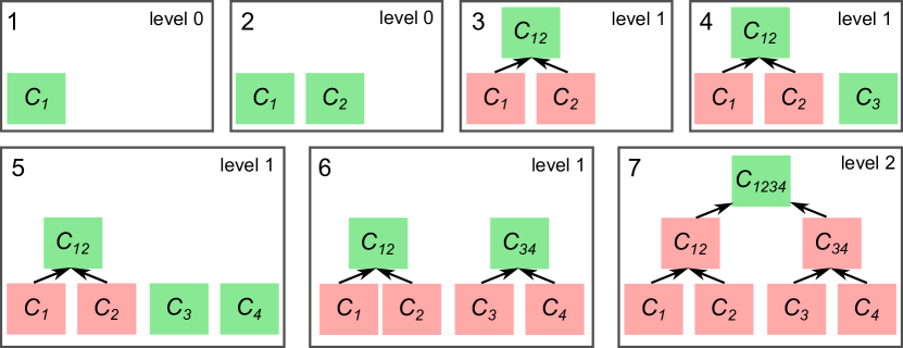
Figure 1: Tree construction: Coresets are constructed using a merge-and-reduce approach. Whenever two coreset nodes are present at the same level, they are merged to construct a higher level coreset (shown in green). The nodes that have been merged are deleted from the memory (shown in red). We prove in Section 3 that the space requirement for tree construction is $\mathcal{O}(\log p(t))$ in the worst case, where $p(t)$ is the number of data points at time $t$, and on average the time complexity is constant per time step.

If $C_{i}$ and $C_{j}$ are two $(1+\epsilon)$ coresets then their concatenation $\left[\frac{C_{i}}{C_{j}}\right]$ is also an $(1+\epsilon)$ coreset. Since

$$\left\|\left[\frac{C_{i}}{C_{j}}\right]Y\right\|_{F}^{2}=\|C_{i}Y\|_{F}^{2}+\|C_{j}Y\|_{F}^{2},$$ (3)

the proof follows trivially from the definition of a coreset. This identity implies that two nodes which are $(1+\epsilon)$ approximation can be concatenated and then re-compressed back to size $n$. This is a key feature of the tree formulation, which repeatedly performs compression from $2n\times d$ to $n\times d$. Each computation can be considered constant in time and space. However, this formulation also reduces the quality of the approximation, since the merged coreset is an $(1+\epsilon)^{2}$ approximation of the two nodes. For every level of the tree, a multiplication error of $(1+\epsilon)$ is introduced from the leaf node to the root.

3.2.1 Data Approximation in the Tree

We denote the entire set up to time $t$ by $\cup_{t}C_{i}$, where $C_{i}$ are the leaves. We denote the coreset tree by $2^{\cup_{t}C_{i}}$. It follows that

Theorem 1.

If $\forall i$ $\tilde{C}_{i}$ is a $(1+\epsilon/q(t))$ approximation of $C_{i}$ then the collapse of the tree $2^{\cup_{t}C_{i}}$ (i.e. the root) is a $(1+\epsilon/3)$ coreset of $\cup_{t}C_{i}$

Proof.

We concatenate and compress sets of two leaves at every level of the tree. Compressing a $2n\times d$ points into $n\times d$ points introduces an additional multiplicative approximation of $(1+\epsilon/q(t))$. Since the maximum depth of the tree at time $t$ is $q(t)$, and

$$\left(1+\frac{\epsilon}{q(t)}\right)^{q(t)}\leq\exp(\epsilon/6)<(1+\epsilon/3),$$ (4)

for $\epsilon<0.1$, we conclude that if we compress $2n\times d$ points to $n\times d$ with an $(1+\epsilon/q(t))$ approximation, the root of the tree will be a $(1+\epsilon/3)$ approximation of the entire data $\cup_{t}C_{i}$. ∎

3.2.2 Space and Time Complexity

We now provide new proofs for the time and space complexity of coreset tree generation per time step and for the entire set.

Theorem 2.

The space complexity to hold a $2^{\cup_{t}C_{i}}$ tree in memory is $\mathcal{O}(ndq(t))$, where $n$ is the size of the coreset of points with dimension $d$.

Proof.

In a coreset tree, two children of the same parent node cannot be in the memory stack simultaneously, which implies that, between two full collapses of the tree, the memory stack is increased at most by $\mathcal{O}(nd)$, which is the size of one leaf. Hence, the space complexity $S(t)$ can be derived as follows –

$$S(n2^{q(t)})=1$$

$$S(p(t))\leq nd+\max_{\hat{p}(t)}S(\hat{p}(t))$$ (5)

$$n2^{q(t)-1}<\hat{p}(t)<n2^{q(t)}\,\,\,\&\,\,\,\ n2^{q(t)}<p(t)<n2^{q(t)+1}$$

This recursive formulation results in a space requirement of $S(p)\leq\mathcal{O}(nd\log(p(t)/n))=\mathcal{O}(ndq(t))$. Assuming $n$ and $d$ are constants chosen a priori, the complexity of the memory is logarithmic in the number of points seen so far. ∎

Theorem 3.

The time complexity of coreset tree construction between time step $t$ and $t+1$ is $\mathcal{O}(\log(p(t)/n)nd^{2})$ in the worst case, which is logarithmic in $p$, the total number of points.

Proof.

In the worst case, we perform $\log(p(t)/n)$ compressions from the lower level all the way to the root. The compressions are performed using SVD. Since the time complexity of each SVD algorithm is $\mathcal{O}(nd^{2})$, assuming $n>d$,

$$T(t+1)-T(t)\leq\mathcal{O}(\log(p(t)/n)nd^{2}) = \mathcal{O}(q(t)nd^{2})$$ (6)

$$= \mathcal{O}(q(t)),$$

where $n$ and $d$ are considered constants. ∎

This scenario occurs for the last data point of a perfect subtree ($p(t)=n2^{q(t)}$).

Finally we wish to explore the total and average time complexity to summarize $p$ points. On average, the time complexity is constant and does not depend on $p$.

Theorem 4.

The time complexity for a complete collapse of a tree to a single coreset of size $n\times d$ is $\mathcal{O}(pd^{2})$, where $d$ the dimension of each point and $p$ is the number of points. The average time complexity per point is constant.

Proof.

$p$ points are split into $p/n$ leaves with $n\times d$ dimension each. The time complexity of SVD is $\mathcal{O}(nd^{2})$, assuming $n>d$. A total of $p(t)/n$ SVDs will be computed for compressing a perfect tree. Hence the total time complexity $T(t)$ for all cycles until time $t$ becomes

$$T(t)=\mathcal{O}\left(\frac{p(t)}{n}nd^{2}\right)=\mathcal{O}(p(t)d^{2})=\mathcal{O}(p(t))$$ (7)

assuming $d$ is constant. We further infer that the average time complexity $\hat{T}(t)$ is $\mathcal{O}(1)$ as

$$\hat{T}(t)=\frac{T(t)}{p(t)}=\mathcal{O}\left(\frac{p(t)d^{2}}{p(t)}\right)=\mathcal{O}(d^{2})=\mathcal{O}(1).$$ (8)

∎

4 CAT: Coreset Adaptive Tracker

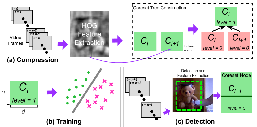
Figure 2: Tracking by detection using coresets: Our system for learning from streaming data contains three main components, which run in parallel. (a) Compression using coresets: For each frame, we extract HoG features from the object. After $n$ frames are processed, a new leaf is inserted into the coreset tree. The tree is compressed recursively by merging nodes at the same level using SVD. (b) Training: A linear SVM for object appearance is trained using data points from the coreset tree after every $n$ frames are processed. The maximum size of the training set is $2n\times d$. (c) Detection: The trained model is used for sliding window detection on every new frame. Features extracted from the detected area are inserted into the coreset tree.

In the previous section, we describe an efficient method to obtain a summarization of all the data till a point in a streaming setting, with strong theoretical guarantees. In this section, we use the coreset tree for tracking by detection using a coreset appearance model for the object.

4.1 Coreset Tree Implementation

The coreset tree is stored as a stack of coreset nodes $S_{C}$. Each coreset node $S_{C}[i]$ has two attributes level and features. level denotes the height of the coreset node in the tree, and features are the image features extracted from a frame. In a streaming setting, once $n$ frames enter the frame stack, we create a coreset node with $level=0$. We merge two coreset nodes when they have the same $level$.

4.2 Coreset Appearance Model

In the coreset tree, any node at level $q$ with size $n$ represents $n2^{q}$ frames, since it is formed after repeatedly merging $2^{q}$ leaf nodes. Nodes with different levels belong to different temporal instances in streaming data. Nodes higher up in the tree have older training samples, whereas a node with level 0 contains the last $n$ frames. This is not ideal for training a tracking system, since more recent frames should have a representation in the learning process. To account for recent data, we propose an hierarchical sampling of the entire tree, constructing an (at most) $2n\times d$-size summarization of the data seen until a given time. For each $S_{C}[i]$ we calculate $w_{i}=2^{(\text{level}(S_{C}[i])-\text{level}(top(S_{C}))}$, and select the first $nw_{i}$ elements from $S_{C}[i]$. This summarized data constitutes our “coreset appearance model”, which is used to train an object detector.

4.2.1 Advantages of Hierarchical Sampling

While the coreset tree formulation has been inspired by Feldman et al. [14], our idea of hierarchical sampling of the entire tree allows to account for recent data, which is crucial for many learning problems which need to avoid a temporal bias in the training set, and especially for tracking by detection. We demonstrate in Table III that hierarchical sampling improves the learning performance significantly as compared to just using the data from the root of the tree.

4.3 System Implementation

In the first frame , user input is used to select a region of interest (ROI) for the object to be tracked. We resize the ROI to a $64\times 64$ square from which we extract $2\times 2$ HOG features from the RGB channels. We also extract HoG features from small affine transformations of the input frame and add them to our frame stack. The affine transformations include scaling, translation and rotation. The number of affine transformations are determined by the number of additional frames required to make the frame stack size reach a maximum of 25% of the total video length. For example, if the coreset size is 5% of the total length of the video, we add 4 transformations per frame. This process gives us the advantage of having more—albeit synthetically generated—samples to train the classifier, and makes the tracker robust to small object scale changes and translations.

Initially, since no coreset appearance model has been trained, we need to use an alternate method for tracking (we use SCM [35] in our current implementation). Once first $n$ frames have been tracked, the first leaf of the tree is formed. Data classification, compression, and training now run in parallel (Figure 2). These components are summarized below –

• Classification: Detect the object in the stream from the last trained classifier.

• Compression: Update a coreset tree, by inserting new leaves and summarizing data whenever possible.

• Training: Train an SVM classifier from the hierarchical coreset appearance model.

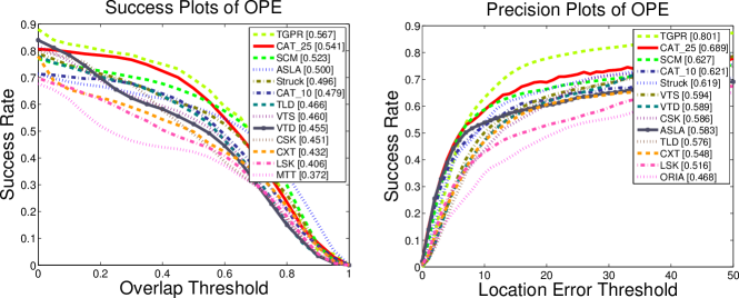
Figure 3: Our methods (CAT_10 and CAT_25) obtains competitive performance on the CVPR2013 Tracking Benchmark on videos with 500 frames or longer. CAT_25 outperforms several top algorithms, such as Struck and SCM.

Algorithm	Mean	Target Type			Target Size		Movement		Occlusion		Motion Type
	Score	Human	Animal	Rigid	Large	Small	Slow	Fast	Yes	No	Active	Passive
CAT_25	0.52	0.52	0.55	0.63	0.49	0.49	0.65	0.38	0.41	0.58	0.59	0.44
TGPR [15]	0.47	0.36	0.51	0.58	0.46	0.48	0.62	0.41	0.35	0.65	0.56	0.44
CAT_10	0.46	0.46	0.49	0.55	0.46	0.45	0.61	0.33	0.30	0.54	0.52	0.40
Struck [19]	0.44	0.35	0.47	0.53	0.45	0.44	0.58	0.39	0.30	0.64	0.54	0.41
VTD [22]	0.45	0.31	0.49	0.54	0.39	0.46	0.57	0.37	0.28	0.63	0.54	0.39
RGB [30]	0.42	0.27	0.41	0.55	0.32	0.46	0.51	0.36	0.35	0.47	0.56	0.34
TLD [21]	0.38	0.29	0.35	0.44	0.32	0.38	0.52	0.30	0.34	0.39	0.50	0.31
MIL [5]	0.37	0.32	0.37	0.38	0.37	0.35	0.46	0.31	0.26	0.49	0.40	0.34

TABLE I: We use the Princeton Tracking Benchmark [30] to compare the precision of CAT with other algorithms using results reported by  [1, 25]. We obtain state of the art results in overall precision and lead the benchmark in 9 out of 11 categories.

Classification

If a classifier has been trained, we feed each sliding window to the classifier and obtain a confidence value. After hard thresholding and non-maximum suppression, we detect an ROI. To remove noise in the position of the ROI, we employ a Kalman filter. We use Expectation Maximization (EM) to obtain its parameters from the centers of the returned predictions of the previous $n$ frames. The EM returns learnt parameters for prediction, which are used to estimate the latent position of the bounding box center. This latent position is used to update the Kalman filter parameters for the next iteration. Once the center of the bounding box is obtained, we calculate the true ROI. We extract features from the ROI and feed it to a feature stack $S_{P}$. Until the first $n$ frames arrive we obtain the ROI from SCM [35] since no classifier has been trained. This process continues till the last frame.

Compression

If $|S_{P}|>n$, we pop the top $n$ elements $S_{P,n}$ from the feature stack and push a coreset node containing elements $S_{P,n}$ into the coreset stack $S_{C}$ with $level=0$. If $level(S_{C}[i])=level(S_{C}[i+1])$, they are merged by constructing a coreset from $S_{C}[i]$ and $S_{C}[i+1]$. We store the coreset in $S_{C}[i]$, and delete $S_{C}[i+1]$. The $level$ for node $S_{C}[i]$ is increased by one. This process continues recursively.

Training

If at least one leaf has been constructed and the size of the coreset stack changes, we train a one-class linear SVM using samples from $S_{C}$. An (at most) $2n\times d$-size appearance model is generated by hierarchical sampling of the tree as described in Section 4.2.

5 Evaluation

We implement the tracking system in C++ with Boost, Eigen, OpenCV, pThreads, and libFreenect libraries. We evaluate the performance of CAT using three publicly available datasets at two coreset sizes—10% and 25%. We denote the tracker with coreset size 10% as CAT_10, and denote the tracker with coreset size 25% as CAT_25.

5.1 CVPR2013 Tracking Benchmark

We first evaluate our algorithm using the CVPR2013 Tracking Benchmark [33] which includes 50 annotated sequences. We use two evaluation metrics to compare the performance of tracking algorithms. The first metric is the precision plot, which shows the percentage of frames whose estimated location is within the given threshold distance of the ground truth. As the representative precision score for each tracker, we use the score for a threshold of 20 pixels. The second metric is the success plot. Given the tracked bounding box $r_{t}$ and the ground truth bounding box $r_{a}$, the overlap score is defined as $S=\frac{|r_{t}\cap r_{a}|}{|r_{t}\cup r_{a}|}$, where $\cap$ and $\cup$ represent the intersection and union of two regions and $|\cdot|$ denotes the number of pixels in the region. We report the success rate as the fraction of frames whose overlap $S$ is larger than some threshold, with the threshold varying from 0 to 1. The area under curve (AUC) of the success plot is used to compare different algorithms.

The strength of our method lies in tracking objects from videos with several hundred frames or longer. So we compare a variety of trackers using videos that are 500 frames or longer (21 out of 50 videos) using the One-Pass Evaluation (OPE) method [33]. Figure 3 shows that we are placed second on this competitive dataset for longer videos in both metrics. We outperform important recent methods including SCM [35] and Struck [19].

5.2 Princeton Tracking Benchmark

The Princeton Tracking Benchmark [30] is a collection of 100 manually annotated RGBD tracking videos, with 214 frames on average. The videos contain significant variation in lighting, background, object size, orientation, pose, motion, and occlusion. The reported score is an average over all frames of precision, which is the ratio of overlap between the ground truth and detected bounding box around the object. We report the performance of all algorithms (including CAT) for RGB data using Princeton Tracking Benchmark evaluation server [1] and from the recent work by Liang et al [25] to ensure consistency in evaluation. CAT_25 obtains state of the art performance on this dataset, and CAT_10 ranks third (Table I). Note that we obtain reasonable precision in presence of occlusions, even though we have no explicit way for occlusion handling. Sample detections are shown in Figure 5.

5.3 TLD Dataset

The coreset formulation summarizes all the data it has seen so far. Therefore we expect the coreset appearance model to adapt to pose and lighting variations as it trains using additional data, and perform well on very long videos. To demonstrate its adaptive behavior, we use the TLD dataset [21], which contains ten videos with $2685$ frames of labeled video on average. For all experiments with the TLD dataset (Tables II, IV, V, and VI) we report the success rate at a threshold of 0.5. Tables II, V, and VI show that CAT_25 significantly outperforms the state of the art, including methods like TGPR [15], which perform better than CAT on the CVPR2013 Tracking Benchmark. CAT_10 is placed third, and it’s success rate is similar to that of TLD. These results support our intuition that the ability of CAT to summarize all data provides a boost in performance over long videos.

5.4 Object Instance Recognition

Since the coreset appearance model learns adaptively from the entire data and does not depend on recency as most tracking methods, it can be used for object instance recognition as well. In a qualitative experiment (Figure 4), we show that a pre-learnt model can be used to detect the same object under varying background, illumination, pose, and deformations.

Algorithm	Success Rate
	Average	Motocross	Panda	VW	Car chase
#Frames	2685	2665	3000	8576	9928
CAT_25	0.66	0.85	0.58	0.67	0.85
TLD [21]	0.57	0.86	0.25	0.67	0.81
CAT_10	0.56	0.77	0.49	0.62	0.79
Struck [19]	0.40	0.57	0.21	0.54	0.31
TGPR [15]	0.38	0.62	0.12	0.62	0.18
SCM [35]	0.36	0.50	0.13	0.47	0.14

TABLE II: CAT obtains state of the art performance on the TLD dataset [21]. We report the average success rate over all videos, as well as success rate for the four longest videos.

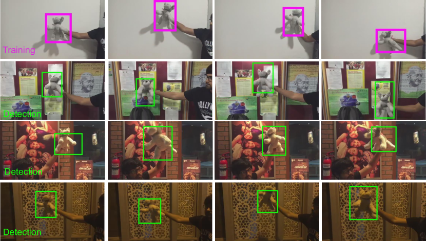
Figure 4: Object instance detection: In a qualitative experiment, we learn the coreset appearance model by tracking an object with plain background in $76$ frames of video (first row). This model can accurately detect and track the same object in different backgrounds (rows 2, 3, 4) and handle illumination changes (rows 3,4).

5.5 Empirical Evaluation of Time Complexity

The coreset formulation is used to train a learning algorithm in constant time and space (Section 3). We compare the time complexity of training with the coreset tree and training using all the data points (Figure 6-(left)). For a linear SVM implementation with linear time complexity [9], the learning time for training with all data points can become prohibitively large, in contrast to the constant, small time needed for learning from coresets. We pay for the reduced cost of training the learning algorithm by the additional time and space requirements of coreset tree formation. We prove in Section 3 that the time complexity of tree construction is constant on average. We validate this result empirically in Figure 6-(right). Other coreset formulations [16] may be used to reduce the space requirements to constant, at the cost of a higher value of the constant for time complexity.

5.6 Comparison with Sampling Methods

In comparison to CAT, sampling can achieve reduction in space and time complexity without the additional overhead of coreset computation. We validate CAT versus random sampling and sub-sampling using the TLD dataset using multiple values of $n$, the coreset size. For random sampling (RS), we use $n$ random frames from all the frames seen so far. For sub-sampling (SS), we use $n$ uniformly spaced frames. CAT consistently outperform both RS and SS (Table IV). Thus, the summarization of data by coresets allows us to learn a more complex object appearance model as compared to sampling.

5.7 Coreset Size Selection

The coreset size $n$ determines the time and space complexity of CAT. In this paper, we evaluate the performance of CAT at coreset sizes which are 10% (CAT_10) or 25% (CAT_25) of the total video size. Using such large values for coreset size is not a strict requirement, but rather an artifact of the datasets used for evaluation. A majority of videos in the three standard datasets are short—114 out of 155 videos have less than 400 frames. We model the object using dense HOG features, which leads to a very high dimensional representation. Hence, the SVM requires sufficient number of data points for good prediction on such short videos. We set $n$ to 10% or 25% of the video size to obtain consistent performance across videos of various sizes.

However, CAT maintains high detection accuracy with small coreset sizes as well. In Table V, we evaluate CAT with various coreset sizes—1%, 2.5%, 5% and 10%—on the TLD dataset. Increasing the coreset size results in an increase in success rate for tracking, since the model captures more information about object appearance. However, the tracking performance is still satisfactory for coreset size as small as 1% of the video size, which is equal to 27 frames on average for the TLD dataset.

Furthermore, CAT performs well, and in fact improves with time, on sufficiently long videos with small coreset sizes that are independent of the number of frames in a video. In Table VI, we compare the performance of CAT with fixed, small coreset size with two top performing methods on extremely long videos. We generate the extremely long videos from the four largest TLD videos by appending clips that are 10% in length of the original video. The clips are randomly flipped, time-reversed, shifted in contrast and brightness, translated by small amounts, and corrupted with Gaussian noise. CAT shows an increase in accuracy with increasing number of frames. In contrast, the success rate of TLD and TGPR reduces with an increase in number of frames. The maximum coreset size in the 100K experiment is 2.5% of the original video. Yet CAT maintains excellent tracking accuracy.

In summary, the impressive performance of CAT—a simple tracker based on appearance models trained with small coreset sizes—in these two experiments demonstrates the utility of the coreset formulation.

Figure 5: Sample detections: We demonstrate excellent performance on the CVPR2013 Tracking Benchmark, the Princeton Tracking Benchmark and the TLD dataset.

Algorithm	Success Rate	Precision
Learning from root of the tree [14]	0.398	0.434
Learning with hierarchical sampling (CAT)	0.524	0.677

TABLE III: Our hierarchical sampling method allows for more representation to recent data in the learning process. In the original formulation [14], the classifier would be trained from the root of the coreset tree alone, ignoring more recent data. We demonstrate that our method provides better accuracy as compared to the original formulation using the CVPR2013 Tracking Benchmark.

Algorithm	% Frames Used For Training
	25	37.5	50	62.5	75
Coreset Size =512
CAT	0.408	0.449	0.483	0.534	0.582
SS	0.332	0.358	0.396	0.408	0.424
RS	0.218	0.221	0.251	0.279	0.301
Coreset Size = 768
CAT	0.502	0.559	0.604	0.637	0.668
SS	0.378	0.415	0.438	0.474	0.502
RS	0.257	0.299	0.326	0.368	0.385
Coreset Size = 1024
CAT	0.546	0.621	0.657	0.701	0.732
SS	0.418	0.492	0.54	0.587	0.633
RS	0.321	0.36	0.381	0.419	0.458

TABLE IV: We show that CAT consistently obtains better success rate than random sampling (RS) and sub-sampling (SS) using the TLD dataset. CAT also shows a greater marginal increase in success rate with increase in $n$ as compared to RS and SS, since it generates a better summarization of the data.

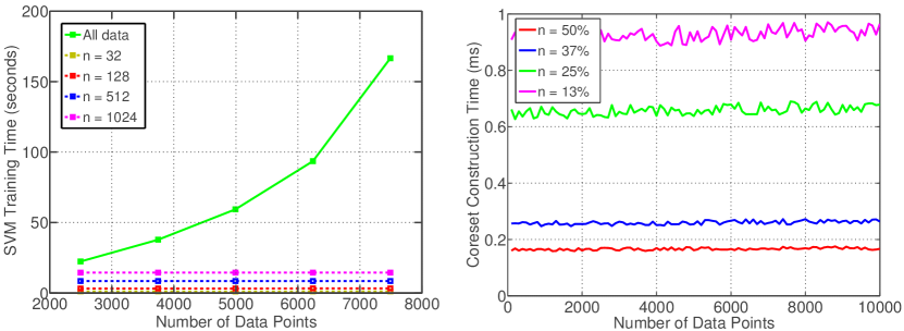
Figure 6: We validate the theoretical bounds for time complexity with empirical analysis using average over all videos from TLD dataset. (Left) The coreset tree allows us to train an SVM in constant time (depending on the coreset size $n$), while the learning time becomes prohibitively large while training with all data points. (Right) The time complexity of coreset construction is constant on average. We demonstrate this at various coreset sizes $n$, expressed as percentage of the total video size, and averaged over all videos in the TLD dataset.

Coreset Size	Success Rate
	Mean	Motocross	VW	Panda	Carchase
1%	0.49	0.74	0.48	0.59	0.73
2.5%	0.51	0.76	0.49	0.59	0.74
5%	0.53	0.77	0.49	0.61	0.74
10% (CAT_10)	0.56	0.77	0.49	0.62	0.79
25% (CAT_25)	0.66	0.85	0.58	0.67	0.85

TABLE V: We evaluate CAT at several coreset sizes as the percent of video size using the TLD dataset. CAT performs satisfactorily at coreset size as small as 1% of the video size.

Algorithm	Number of Frames
	10K	20K	50K	75K	100K
CAT (n=500)	0.522	0.559	0.578	0.586	0.594
CAT (n=1000)	0.606	0.634	0.658	0.669	0.673
CAT (n=1500)	0.627	0.674	0.697	0.701	0.702
CAT (n=2000)	0.685	0.702	0.718	0.725	0.726
CAT (n=2500)	0.713	0.724	0.736	0.743	0.744
TLD [21]	0.579	0.573	0.569	0.567	0.567
TGPR [15]	0.382	0.368	0.365	0.364	0.362

TABLE VI: Success Rate Comparison: CAT performs well, and in fact improves with time, on very long videos with small, fixed coreset size which is independent of the total number of frames.

6 Discussion

Tracking in Long Videos: A majority of tracking algorithms are unable to directly make use of data from all the previous frames. At best, they retain a few ‘good’ frames to learn [31] or maintain an auxiliary set of earlier frames [15]. Our method can retain a summary of all frames seen so far using logarithmic space with an efficient algorithm. This is an important advantage for practical systems with space and time constraints.

Simplicity: The utility of the coreset formulation is evident from the fact that we obtain state of the art experimental results with a simple tracker that consists of a linear classifier and a Kalman filter. The primary goal of this work is to explore the benefit of coresets for learning from streaming visual data, rather than to compete on tracking benchmarks. Additional improvement could be obtained via choosing the optimal coreset size or exploring various hierarchical sampling methods. Performance may also improve by incorporating traditional methods for handling occlusion and drift.

Real-time Performance: Our current implementation, running on commodity hardware (Intel i7 Processor, 8 GB RAM), performs coreset construction and SVM training in parallel at $\scriptstyle\sim$20 FPS for small coreset sizes ($n\leq 64$). Due to the high computational complexity of sliding window detection, the total speed is $\scriptstyle\sim$3 FPS. Faster detection methods (e.g., efficient subwindow search [23] and parallelization [32]) can be easily incorporated into our system to achieve real-time performance.

7 Concluding Remarks

In this paper, we proposed an efficient method for training object appearance models using streaming data. The key idea is to use coresets to compress object features through time to a constant size and perform learning in constant time using hierarchical sampling of coresets. Our method is ideal for efficient tracking in long videos in real world scenarios. Since we maintain a compact summary of all previous data, our learning model improves with time. We provide experimental validation for this insight with strong performance on the TLD dataset which contains videos with $2685$ frames on average. The ideas described in this paper complement the current expertise in the computer vision community on developing trackers and detectors. Combining our framework with existing methods should lead to fruitful online approaches, particularly when ‘old’ data should be taken into account. While we explore the use of coresets for object tracking in this paper, we hope that our technique can be adapted for a variety of applications, such as image collection summarization, video summarization and more.

References

- [1] The Princeton Tracking Benchmark Evaluation Server. http://tracking.cs.princeton.edu/eval.php. Accessed: 2015-04-20.
- [2] P. K. Agarwal, S. Har-Peled, and K. R. Varadarajan. Approximating extent measures of points. Journal of the ACM, 51(4):606–635, 2004.
- [3] S. Avidan. Support vector tracking. IEEE Transactions on Pattern Analysis and Machine Intelligence, 26(8):1064–1072, 2004.
- [4] S. Avidan. Ensemble tracking. IEEE Transactions on Pattern Analysis and Machine Intelligence, 29(2):261–271, 2007.
- [5] B. Babenko, M.-H. Yang, and S. Belongie. Robust object tracking with online multiple instance learning. IEEE Transactions on Pattern Analysis and Machine Intelligence, 33(8):1619–1632, 2011.
- [6] M. Bādoiu, S. Har-Peled, and P. Indyk. Approximate clustering via core-sets. ACM Symposium on Theory of Computing, pages 250–257, 2002.
- [7] J. Bentley and J. Saxe. Decomposable searching problems i: Static-to-dynamic transformation. Journal of Algorithms, 1(4):301–358, 1980.
- [8] M. J. Black and A. D. Jepson. Eigentracking: Robust matching and tracking of articulated objects using a view-based representation. European Conference on Computer Vision, pages 329–342, 1996.
- [9] C.-C. Chang and C.-J. Lin. LIBSVM: a library for support vector machines. ACM Transactions on Intelligent Systems and Technology, 2(3):27, 2011.
- [10] K. L. Clarkson and D. P. Woodruff. Numerical linear algebra in the streaming model. ACM Symposium on Theory of Computing, 2009.
- [11] D. Comaniciu, V. Ramesh, and P. Meer. Kernel-based object tracking. IEEE Transactions on Pattern Analysis and Machine Intelligence, 25(5):564–577, 2003.
- [12] D. Feldman, S. Gil, R. Knepper, B. Julian, and D. Rus. K-robots clustering of moving sensors using coresets. IEEE International Conference on Robotics and Automation, pages 881–888, 2013.
- [13] D. Feldman, M. Monemizadeh, and C. Sohler. A PTAS for k-means clustering based on weak coresets. ACM Symposium on Computational Geometry, pages 11–18, 2007.
- [14] D. Feldman, M. Schmidt, and C. Sohler. Turning big data into tiny data: Constant-size coresets for k-means, PCA and projective clustering. ACM-SIAM Symposium on Discrete Algorithms, pages 1434–1453, 2013.
- [15] J. Gao, H. Ling, W. Hu, and J. Xing. Transfer learning based visual tracking with gaussian processes regression. European Conference on Computer Vision, pages 188–203, 2014.
- [16] M. Ghashami and J. M. Phillips. Relative errors for deterministic low-rank matrix approximations. ACM-SIAM Symposium on Discrete Algorithms, 2014.
- [17] H. Grabner, C. Leistner, and H. Bischof. Semi-supervised on-line boosting for robust tracking. European Conference on Computer Vision, pages 234–247, 2008.
- [18] S. Har-Peled and S. Mazumdar. On coresets for k-means and k-median clustering. ACM Symposium on Theory of Computing, 2004.
- [19] S. Hare, A. Saffari, and P. H. Torr. Struck: Structured output tracking with kernels. IEEE Internation Conference on Computer Vision, pages 263–270, 2011.
- [20] A. D. Jepson, D. J. Fleet, and T. F. El-Maraghi. Robust online appearance models for visual tracking. IEEE Transactions on Pattern Analysis and Machine Intelligence, 25(10):1296–1311, 2003.
- [21] Z. Kalal, K. Mikolajczyk, and J. Matas. Tracking-learning-detection. IEEE Transactions on Pattern Analysis and Machine Intelligence, 34(7):1409–1422, 2012.
- [22] J. Kwon and K. M. Lee. Visual tracking decomposition. IEEE Conference on Computer Vision and Pattern Recognition, pages 1269–1276, 2010.
- [23] C. H. Lampert, M. B. Blaschko, and T. Hofmann. Beyond sliding windows: Object localization by efficient subwindow search. IEEE Conference on Computer Vision and Pattern Recognition, pages 1–8, 2008.
- [24] H. Li, C. Shen, and Q. Shi. Real-time visual tracking using compressive sensing. IEEE Conference on Computer Vision and Pattern Recognition, pages 1305–1312, 2011.
- [25] P. Liang, C. Liao, X. Mei, and H. Ling. Adaptive objectness for object tracking. arXiv preprint arXiv:1501.00909, 2015.
- [26] E. Liberty. Simple and deterministic matrix sketching. ACM Conference on Knowledge Discovery and Data Mining, 2013.
- [27] G. Rosmanm, M. Volkov, D. Feldman, W. Fisher, and D. Rus. Coresets for k-segmentation of streaming data. Advances in Neural Information Processing Systems, 2014.
- [28] D. A. Ross, J. Lim, R.-S. Lin, and M.-H. Yang. Incremental learning for robust visual tracking. International Journal of Computer Vision, 77(1-3):125–141, 2008.
- [29] A. W. M. Smeulders, D. M. Chu, R. Cucchiara, S. Calderara, A. Dehghan, and M. Shah. Visual tracking: An experimental survey. IEEE Transactions on Pattern Analysis and Machine Intelligence, 2014.
- [30] S. Song and J. Xiao. Tracking revisited using RGBD camera: Unified benchmark and baselines. IEEE Internation Conference on Computer Vision, pages 233–240, 2013.
- [31] J. Supancic and D. Ramanan. Self-paced learning for long-term tracking. IEEE Conference on Computer Vision and Pattern Recognition, pages 2379–2386, 2013.
- [32] C. Wojek, G. Dorkó, A. Schulz, and B. Schiele. Sliding-windows for rapid object class localization: A parallel technique. Pattern Recognition, pages 71–81, 2008.
- [33] Y. Wu, J. Lim, and M.-H. Yang. Online object tracking: A benchmark. IEEE Conference on Computer Vision and Pattern Recognition, pages 2411–2418, 2013.
- [34] K. Zhang, L. Zhang, and M.-H. Yang. Real-time compressive tracking. European Conference on Computer Vision, pages 864–877, 2012.
- [35] W. Zhong, H. Lu, and M.-H. Yang. Robust object tracking via sparsity-based collaborative model. IEEE Conference on Computer Vision and Pattern Recognition, pages 1838–1845, 2012.