Principled Parallel Mean-Field Inference for Discrete Random Fields

Abstract

Mean-field variational inference is one of the most popular approaches to inference in discrete random fields. Standard mean-field optimization is based on coordinate descent and in many situations can be impractical. Thus, in practice, various parallel techniques are used, which either rely on ad hoc smoothing with heuristically set parameters, or put strong constraints on the type of models.

In this paper, we propose a novel proximal gradient-based approach to optimizing the variational objective. It is naturally parallelizable and easy to implement.

We prove its convergence, and then demonstrate that, in practice, it yields faster convergence and often finds better optima than more traditional mean-field optimization techniques. Moreover, our method is less sensitive to the choice of parameters.

1 Introduction

Many Computer Vision problems, ranging from image segmentation to depth estimation from stereo, can be naturally formulated in terms of Conditional Random Fields (CRFs). Solving these problems then requires either estimating the most probable state of the CRF, or the marginal distributions over the unobserved variables. Since there are many such variables, it is usually impossible to get an exact answer, and one must instead look for an approximation.

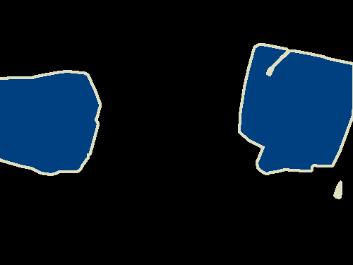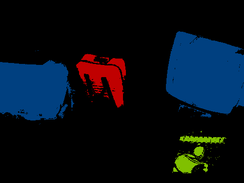
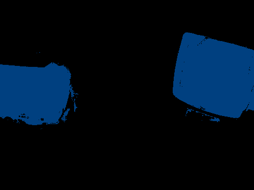
input	baseline	ours	ground truth

Figure 1: First three rows: VOC2012 images in which we outperform a baseline by adding simple co-ocurrence terms, which our optimization scheme, unlike earlier ones, can handle. Bottom row: Our scheme also allows us to improve upon a baseline for the purpose of recovering a character from its corrupted version.

Mean-field variational inference [31] is one of the most effective ways to do approximate inference and has become increasingly popular in our field [27, 30, 22]. It involves introducing a variational distribution that is a product of terms, typically one per hidden variable. These terms are then estimated by minimizing the Kullback-Leibler (KL) divergence between the variational and the true posterior. The standard scheme is to iteratively update each factor of the distribution one-by-one. This is guaranteed to converge [5, 19], but is not very scalable, because all variables have to be updated sequentially. It becomes impractical for realistically-sized problems when there are substantial interactions between the variables. This can be remedied by replacing the sequential updates by parallel ones, often at the cost of failing to converge.

It has nonetheless recently been shown that parallel updates could be done in a provably convergent way for pairwise CRFs, provided that the potentials are concave [22]. When they are not, an ad hoc heuristic designed to achieve convergence, which essentially smooths steps by averaging between the next and current iterate, has been used over the years. This heuristic is mentioned explicitly in some works [28, 7, 13], or used implicitly in optimization schemes [12, 30] by introducing an additional damping parameter.

However, a formal justification for such smoothing is never provided, which we do in this paper. More specifically, we show that, by damping in the natural parameter space instead of the mean-parameter one, we can reformulate the optimization scheme as a specific form of proximal gradient descent. This yields a theoretically sound and practical way to chose the damping parameters, which guarantees convergence, no matter the shape of the potentials. When they are attractive, we show that our approach is equivalent to that of [22]. However, even when they are repulsive and can cause the earlier methods to oscillate without ever converging, our scheme still delivers convergence. For example, as shown in Fig. 1, this allows us to add co-occurrence terms to the model used by a state-of-the-art semantic segmentation method [8] and improves its results. Furthermore, we retain the simplicity of the closed-form mean-field update rule, which is one of the key strengths of the mean-field approach.

In short, our contribution is threefold:

• We introduce a principled, simple, and efficient approach to performing parallel inference in discrete random fields. We formally prove that it converges and demonstrate that it performs better than state-of-the-art inference methods on realistic Computer Vision tasks such as segmentation and people detection.

• We show that many of the earlier methods can be interpreted as variants of ours. However, we offer a principled way to set its metaparameters.

• We demonstrate how parallel mean-field inference in random fields relates to the gradient descent. This allows us to integrate advanced gradient descent techniques, such as momentum and ADAM [18], which makes mean-field inference even more powerful.

To validate our approach, we first evaluate its performance on a set of standardized benchmarks, which include a range of inference problems and have recently been used to assess inference methods [13]. We then demonstrate that the performance improvements we observed carry over to three realistic Compute Vision problems, namely Characters Inpainting, People Detection and Semantic Segmentation. In each case, we show that modifying the optimization scheme while retaining the objective function of state-of-the-art models [12, 25, 8] yields improved performance and addresses the convergence issues that sometimes arise [30].

2 Background and Related Work

In this section, we briefly review basic Conditional Random Field (CRF) theory and the use of mean-field inference to solve the resulting optimization problems. We also give a short introduction into proximal gradient descent algorithms, on which our method is based. Note, in this work, we focus on models involving discrete random variables.

2.1 Conditional Random Fields

Let $\mathbf{X}=\left(X_{1},\ldots,X_{N}\right)$ represent hidden variables and $\bm{I}$ represent observed variables. For example, for semantic segmentation, the $X_{i}$s are taken to be variables representing semantic classes of $N$ pixels, and $\bm{I}$ represents the observed image evidence.

A Conditional Random Field (CRF) models the relationship between $\mathbf{X}$ and $\mathbf{I}$ in terms of the posterior distribution

$$\vspace{-0.1cm}P(\mathbf{X}\mid\mathbf{I})=\exp\left(\sum_{c\subset\{1,\dots,N\}}\bm{\phi}_{c}(\mathbf{X}_{c}\mid\mathbf{I})-\log Z(\mathbf{I})\right)\;,$$ (1)

where $\bm{\phi}_{c}(.)$ are non-negative functions known as potentials and $\log Z(\mathbf{I})$ is the log-partition function. It is a constant that we will omit for simplicity since we are mostly concerned by estimating values of $\mathbf{X}$ that maximize $P(\mathbf{X}\mid\mathbf{I})$.

This model is often further simplified by only considering unary and pairwise terms:

$$\vspace{-0.1cm}P(\mathbf{X}\mid\mathbf{I})\propto\exp\left(\sum_{i}\phi_{i}(X_{i},I_{i})+\sum_{(i,j)}\phi_{ij}(X_{i},X_{j})\right).$$ (2)

2.2 Mean-Field Inference

Typically, one wants either to estimate the posterior $P(\mathbf{X}|\mathbf{I})$ or to find the vector $\hat{\mathbf{X}}$ that maximizes $P(\mathbf{X}|\mathbf{I})$, which is known as the MAP assignment. Unfortunately, even for the simplified formulation of Eq. 2, both are intractable for realistic sizes of $\mathbf{X}$. As a result, many approaches settle for approximate solutions. These include sampling methods, such as Gibbs sampling [14], and deterministic ones such as mean-field variational inference [32], belief propagation [24, 23, 20], and others [6, 15].

Note that, mean-field methods have been shown to combine the advantages of good convergence guarantees [5], flexibility with respect to the potential functions that can be handled [27], and potential for parallelization [22]. As a result, they have become very popular in our field. Furthermore, they have recently been shown to yield state-of-the-art performance for several Computer Vision tasks [27, 30, 8, 33].

Mean-field involves introducing a distribution $Q$ of the factorized form

$$\vspace{-0.1cm}Q(\mathbf{X}=(x_{1},\ldots,x_{N});\mathbf{q})=\prod_{i=1}^{N}Q_{i}(X_{i}=x_{i};\mathbf{q}_{i})\;,$$ (3)

where $Q_{i}(\,.\,;\mathbf{q}_{i})$ is a categorical distribution with mean parameters $\mathbf{q}_{i}$. That is,

$$\forall l,\,Q_{i}(X_{i}=l;\mathbf{q}_{i})=q_{i,l},$$ (4)

with $\mathbf{q}$ on the simplex $\mathcal{M}$ such that $\forall i,l,\;0\leq q_{i,l}\leq 1$ and $\forall i,\sum_{l}q_{i,l}=1$.

$Q$ is then used to approximate $P(\mathbf{X}\mid\mathbf{I})$ by minimizing the KL-divergence:

$$\text{KL}(Q||P)=\sum_{\bm{x}}Q(\mathbf{X}=\mathbf{x};\mathbf{q})\log\frac{Q(\mathbf{X}=\mathbf{x};\mathbf{q})}{P(\mathbf{X}=\mathbf{x}\mid\mathbf{I})}\;.$$ (5)

In some cases, this approximation is the desired final result. In others, one seeks a MAP assignment. To this end, a standard method is to select the assignment that maximizes the approximate posterior $Q(\mathbf{X};\mathbf{q})$, which is equivalent to rounding when the $X_{i}$s are Bernoulli variables. An alternative approach is to draw samples from $Q(\mathbf{X};\mathbf{q})$.

When minimizing the KL-divergence of Eq. 5, $Q(\mathbf{X};\mathbf{q})$ can be reparameterized in terms of its natural parameters defined as follows. For each variable $X_{i}$ and label $l$, we take the natural parameter $\theta_{i,l}$ to be such that

$$Q(X_{i}=l;\mathbf{q}_{i})=q_{i,l}\propto\exp[-\theta_{i,l}].$$ (6)

As we will see below, this typically yields simpler notations and implementations.

2.2.1 Sweep Mean-Field Inference

Solving the minimization problem of Eq. 5 is equivalent [5] to minimizing

$$\mathcal{F}(\mathbf{q})=\underbrace{-\mathbf{E}_{Q(\bm{X};\mathbf{q})}[\log P(\mathbf{X}\mid\mathbf{I})]}_{\mathcal{E}(\mathbf{q})}+\underbrace{\mathbf{E}_{Q(\bm{X};\mathbf{q})}[\log Q(\bm{X};\mathbf{q})]}_{-\mathcal{H}(\mathbf{q})},$$ (7)

with respect to $\mathbf{q}$ on the simplex $\mathcal{M}$. $\mathcal{F}(.)$ is sometimes called the variational free energy. Its first term is the expectation of the energy under $Q(\mathbf{X};\mathbf{q})$, and its second term is the negative entropy, which acts as a regularizer.

One can minimize $\mathcal{F}(\mathbf{q})$ by iteratively updating each $q_{i,l}$ in sequence while keeping the others fixed. Each update involves setting $q_{i,l}$ to

$$q^{\star}_{i,l}\propto\exp\left[\mathbf{E}_{Q(\mathbf{X}/X_{i};\mathbf{q})}\big{[}\log P(\mathbf{X}\mid\mathbf{I})\big{]}\right].$$ (8)

This coordinate descent procedure, which we will call SWEEP, is guaranteed to converge to a local minimum of $\mathcal{F}$ [5]. However, it tends to be very slow for realistic image sizes and impractical for many Computer Vision problems [30, 22]. Namely, in the case of dense random fields, it involves re-computing a large number of expectations (one per factor adjacent to the variable) after each sequential update. Filter-based mean-field inference [21] attempts to reduce the complexity of these updates, but it effectively performs parallel updates, which we will describe below.

2.2.2 Parallel Mean-Field Inference

To obtain reasonable efficiency in practice, Computer Vision practitioners often perform the updates of Eq. 8 in parallel as opposed to sequentially. Not only does it avoid having to reevaluate a large number of factors after each update, it also allows the use of vectorized instructions and GPUs, both of which can have a dramatic impact on the computation speed.

Unfortunately, these parallel updates invalidate the convergence guarantees and in practice often lead to undesirable oscillations in the objective. Several approaches to remedying this problem have been proposed, which we review below.

Damping

A natural way to improve convergence is to replace the updates of Eq. 8 by a damped version, expressed as

$$q_{i,l}^{t+1}=(1-\eta)\cdot q_{i,l}^{t}+\eta\cdot q_{i,l}^{\star}\;,$$ (9)

where $t$ denotes the current iteration, $q_{i,l}^{\star}$ is the result of solving the optimization problem of Eq. 8, and $\eta$ is a heuristically chosen damping parameter. This damping is explicitly mentioned in papers such as [7, 28, 13]. In [30], convergence issues are mentioned and a damping parameter is provided in the publicly available code. Similarly, in [12], the algorithm relies on mean-field optimization with repulsive terms. The need for damping is not explicitly discussed in the paper, but the publicly available code also includes a damping.

Damping delivers satisfactory results in many cases, but does not formally guarantee convergence. It may fail if the parameter $\eta$ is not carefully chosen, and sometimes changed at different stages of the optimization. In all the approaches that we are aware of, this is done heuristically. We will refer to this type of methods as ADHOC.

Concave potentials

A principled way to address the convergence issue for the pairwise random fields is offered in [22], and we refer to the corresponding algorithm as FULL-PARALLEL. However, authors restrict their potentials $\phi_{ij}$ of Eq. 2 to be concave, which in some cases is reasonable, but as we will show in Section 4, many Computer Vision models violate this requirement. By contrast, our approach is similarly principled but without additional constraints. In practice it works for higher-order, or, equivalently, non-pairwise potentials.

2.3 Proximal Gradient Descent

Let $F$ be a generic objective function of the form $F(\mathbf{x})=f(\mathbf{x})+g(\mathbf{x})$, where $g$ is a regularizer, and $\mathbf{x}_{t}$ is the value of the optimized variable at iteration $t$ of a minimization procedure on a constraint set $\mathcal{X}$. Proximal gradient descent, also known as composite mirror-descent [10], is an iterative method that relies on the update rule

$$\mathbf{x}^{t+1}=\operatorname*{\arg\!\min}_{\mathbf{x}\in\mathcal{X}}\{\langle\mathbf{x},\nabla f(\mathbf{x}^{t})\rangle+g(\mathbf{x})+\lambda\Psi(\mathbf{x},\mathbf{x}^{t})\}\;\;,$$ (10)

where $\Psi$ is a non-negative proximal function that satisfies $\Psi(\mathbf{x},\mathbf{x}^{t})=0$ if and only if $\mathbf{x}=\mathbf{x}^{t}$, and $\lambda$ is a scalar parameter. $g$ contains the terms of the objective function that do not need to be approximated to the first order, while still allowing efficient computation of update of Eq. 10. $\Psi$ can be understood as a distance function that accounts for the geometry of $\mathcal{X}$ [29] while also making it possible to compute the update of Eq. 10 efficiently. $\lambda$ can then be thought of as the inverse of the step size.

As shown in Section 3.1, our algorithm is a version of proximal gradient descent in which $\Psi$ is based on the KL-divergence and allows automated step-size adaptation as the optimization progresses. Recently, a variational approach that also relies on the KL-divergence as the proximal function has been proposed [17]. This paper explores the connection between the KL-proximal method and the Stochastic Variational Inference [1, 16]. However, it does not allow for step size adaptation, which often yields better performance, as we demonstrate in our experiments and is not directly applied to the mean-field setting.

3 Method

As discussed in the previous section, the goal of mean-field inference is to

$$\underset{\mathbf{q}\in\mathcal{M}}{\text{minimize }}\mathcal{F}(\mathbf{q})$$ (11)

where $\mathcal{F}$ is the variational free energy of Eq. 7. Performing sequential updates of the $q_{i,l}$ is guaranteed to converge, but can be slow. Parallel updates are usually much faster, but the optimization procedure may fail to converge.

In this section, we introduce our approach to guaranteeing convergence whatever the shape of the pairwise potentials. To this end, we rely on proximal gradient descent as described in Section 3.1 and formulate the proximal function $\Psi$ in terms of the KL-divergence. This is motivated by the fact that it is more adapted to measuring the distance between probability distributions than the usual L2 norm, while being independent of how the distribution is parameterized.

We will show that this both guarantees convergence and yields a principled way to obtain a closed form damped update equation equivalent to Eq. 9.

3.1 Proximal Gradient for Mean-Field Inference

In our approach to minimizing the variational free energy of Eq. 7, we treat $\mathcal{E}$ as the function $f$ of Eq. 10 and the negative entropy $-\mathcal{H}$ as the regularizer $g$. This choice stems from the fact that $-\mathcal{H}$ is separable, and therefore, can be minimized in parallel in Eq. 10, without using a first order approximation. Also, $-\mathcal{H}$ being the regularizer $g$ means that we do not need to look at its derivatives with respect to the mean-parameters, which are not well behaved when they approach zero. We then define

$$\Psi^{t}(\mathbf{q},\mathbf{q}^{t})=\sum\limits_{i}\sum\limits_{l}d^{t}_{i,l}q_{i,l}\log\dfrac{q_{i,l}}{q_{i,l}^{t}}=\mathbf{D}^{t}\odot\text{KL}(\mathbf{q}||\mathbf{q}^{t})\;,$$ (12)

where KL is the non-negative KL-divergence, which is a natural choice for a distance between distributions. $\mathbf{D}^{t}$ is a diagonal matrix with positive diagonal elements $d^{t}_{i,l}$s, which we introduce to allow for anisotropic scaling of the proximal KL-divergence term. As will be discussed below, different choices of the $d^{t}_{i,l}$s yield different variants of our algorithms. Note however that, $\Psi^{t}$ is a valid proximal function.

The update of Eq. 10 then becomes

$$\mathbf{q}^{t+1}=\operatorname*{\arg\!\min}_{\mathbf{q}\in\mathcal{M}}\{\langle\mathbf{q},\nabla\mathcal{E}(\mathbf{q}^{t})\rangle-\mathcal{H}(\mathbf{q})+\mathbf{D}^{t}\odot\text{KL}(\mathbf{q}||\mathbf{q}^{t})\}\;.$$ (13)

This computation can be performed independently for each index $i\in\{1,\dots,N\}$. Furthermore, we prove in the supplementary material that it can be done in closed form and can be written as

$$q_{i,l}^{t+1} \propto\exp[ \eta^{t}_{i,l}\cdot\mathbf{E}_{Q(\mathbf{X}/X_{i}=l;\mathbf{q})}\big{[}\log P(\mathbf{X}|\mathbf{I})\big{]}$$

$$+(1-\eta^{t}_{i,l})\cdot\log q_{i,l}^{t}]\;,$$

where $\eta^{t}_{i,l}=\dfrac{1}{1+d^{t}_{i,l}}$. Eq 3.1 can be rewritten as

$$\theta_{i,l}^{t+1}=\eta^{t}_{i,l}\cdot\theta_{i,l}^{\star}+(1-\eta^{t}_{i,l})\cdot\theta_{i,l}^{t}\;\;,$$ (15)

where $\theta_{i,l}^{\star}=-\mathbf{E}_{Q(\mathbf{X}/X_{i};\mathbf{q})}\big{[}\log P(\mathbf{X}|\mathbf{I})\big{]}$ now is a natural parameter, like those of Eq. 6. In other words, we have replaced the heuristic update rule of Eq. 9 in the space of mean parameters by a principled one in the space of natural ones. As we will see, this yields performance and convergence improvements in most cases. As for the stopping criteria, one can define one based on the value of the objective, or, in practice, run inference for a fixed number of iterations.

3.2 Fixed Step Size

The simplest way to instantiate our algorithm is to fix all the $d^{t}_{i,l}$s of Eq. 12 to the same value $d$ and to write

$$\forall t\;,\;\mathbf{D}^{t}=\mathbf{D}=d\mathbb{I}\;\Rightarrow\;\forall t,i,l,\eta^{t}_{i,l}=\dfrac{1}{1+d}\;,$$ (16)

where $\eta^{t}_{i,l}$ plays the same role as the damping factor of Eq. 9. We now show that this is guaranteed to converge when the proximal term is given enough weight.

In our mean-field settings, $\mathcal{E}(\mathbf{q})$ is a polynomial function of the mean-parameters vector $\mathbf{q}$. Therefore, one can always find some positive real number $L$ such that $\mathcal{E}$ is L-Lipschitz gradient, which means

$$\forall x,y\in\mathcal{M}\;,\;\|\nabla\mathcal{E}(x)-\nabla\mathcal{E}(y)\|_{2}\leq L\|x-y\|_{2}\;.$$ (17)

In the supplementary material, we prove that this property implies that our proximal gradient descent scheme is guaranteed to converge for any fixed matrix $D=d\mathbb{I}$ such that $d>L$.

Intuitively, when updating the value of $\mathbf{q}^{t}$ to $\mathbf{q}^{t+1}$, the magnitude of the gradient change controlled and thus the coordinate-wise optimum $\theta_{i,l}^{\star}=-\nabla\mathcal{E}(\mathbf{q}^{t})_{i,l}$ will also be changing smoothly across iterations. As a result, $L$ is the key value to understand oscillations. In practice, our goal is to find its smallest possible value to allow steps as large as possible while guaranteeing convergence.

In the pairwise case, the Hessian of the objective function is a constant matrix, which we call potential matrix. Therefore, the highest eigenvalue of the potential matrix is a valid Lipschitz constant and efficient methods allow to compute it for moderately sized problems.

In fact, the convergence result presented in [22] is strongly related to this. Namely, assuming that the potential matrix is negative semi-definite, is equivalent to assuming that $L<0$ in our formulation. This directly corresponds to the concavity assumptions on the potentials in [22]. Therefore, under the assumptions of [22], our algorithm leads to $\eta=1$, corresponding to the fully-parallel update procedure. In that sense, our procedure is a generalization of the one proposed by [22].

In the non-pairwise case, the Hessian is not constant, and the calculation of the Lipschitz constant is not trivial. For each specific problem, bounds should be derived using the particular shape of the CRF at hand.

3.3 Adaptive Step Size

Note that the Hessian of the KL-proximal term is diagonal with

$$\dfrac{\partial^{2}\mathbf{D}^{t}\cdot\text{KL}(\mathbf{q}||\mathbf{q}^{t})}{\partial q_{i,l}^{2}}|_{\mathbf{q}=\mathbf{q}^{t}}=\dfrac{d^{t}_{i,l}}{q^{t}_{i,l}}\;.$$ (18)

Therefore, when some of the $q_{i,l}$s get close to 0, the elements of the Hessian may become very large, especially when using a constant value for the $d^{t}_{i,l}$ as suggested above. When that happens, the local KL-approximation remains a valid upper bound of the objective function, but not a tight enough one, which results in step sizes that are too small for fast convergence.

This can be reduced by choosing a matrix $\mathbf{D}^{t}$ that compensates for this. A simple way to do this would be to scale the $d_{i,l}^{t}$ proportionally to $\max(q_{i,0},\dots,q_{i,L_{i}-1})$ to start compensating for diagonal terms. However, this method is still sub-optimal because it ignores the fact that all our variables lie inside the simplex $\mathcal{M}$. A better alternative is to bound from below the proximal term by a quadratic function, but on $\mathcal{M}$ rather than on $\mathbb{R}^{n}$.

In this paper, we only apply this method to the binary case, for which we set

$$d^{t}_{i,0}=d^{t}_{i,1}=q^{t}_{i,0}q^{t}_{i,1}\cdot d\;,$$ (19)

were $d$ is an additional parameter that should be set close to $L$. Extending this approach to the multi-label case will be a topic for future work. In Section 3.4, we provide a different alternative to performing adaptive anisotropic updates in all settings.

Intuitively, when the current parameters are close to the borders of the simplex, the mean parameters are less sensititive to natural parameters, which, therefore, need less damping. We demonstrate in our experiments that it provides a way to choose the step size without tuning.

3.4 Momentum

Our approach can easily be extended to incorporate techniques that are known to speed-up gradient descent and help to avoid local minima, such as the classic momentum method [26] or the more recent ADAM technique [18]. The momentum method involves averaging the gradients of the objective $f(\mathbf{x})$ over the iterations in a momentum vector $\mathbf{m}$ and use it as the direction for the update instead of simply following the current gradient. To integrate it into our framework, we replace the gradient $\nabla\mathcal{E}$ in Eq. 13 by its rolling exponentially weighted average $\mathbf{m}$ computed as

$$\mathbf{m}^{t+1} = \gamma_{1}\mathbf{m}^{t}+(1-\gamma_{1})\nabla\mathcal{E}(\mathbf{q}^{t})\;,$$ (20)

with the exponential decay parameter $\gamma_{1}\in[0;1]$. This substitution brings the following update rule

$$\theta_{i,l}^{t+1} = \eta\cdot m_{i,l}^{t}+(1-\eta)\cdot\theta_{i,l}^{t}\;.$$ (21)

We will refer to this approach as OURS-MOMENTUM.

3.5 ADAM

The ADAM method [18] has become very popular in deep learning. Our framework makes it easy to use for mean-field inference as well by appropriately choosing the matrix $\mathbf{D}^{t}$ at each step and combining it with the momentum technique.

We define the averaged second moment vector $\mathbf{v}$ of the natural gradient as

$${v}^{t+1}_{i,l} = \gamma_{2}[\theta^{t}_{i,l}+\nabla\mathcal{E}(\mathbf{q}^{t})_{i,l}]^{2}+(1-\gamma_{2}){v}^{t}_{i,l}\;,$$ (22)

where $\mathbf{v}$ is initialised to a strictly positive value and $\gamma_{2}\in[0;1]$ is an exponential memory parameter for $\mathbf{v}$.

Then, the $\mathbf{D}^{t}$ matrix is defined through each of its diagonal entries as

$$d^{t}_{i,l}=\sqrt{{v}^{t+1}_{i,l}}d+\epsilon-1\;,$$ (23)

where $\epsilon$ is a fixed parameters and $d$ controls the damping. We will refer to this method as OURS-ADAM.

Intuitively it is good at exploring parameter space thanks to a form of auto-annealing of the gradient. The natural gradient $\mathbf{\theta}_{t}+\nabla\mathcal{E}(\mathbf{q}^{t})$ is zero at a local minimum of the objective function [16]. Therefore, close to a minimum, the proximal term $\mathbf{D}^{t}$ becomes small, thus allowing more exploration of the space. On the other hand, after a long period of exploration with large natural gradients, more damping will tend to make the algorithm converge.

4 Experimental Evaluation

In this section, we evaluate our method on a variety of inference problems and demonstrate that in most cases it yields faster convergence and better minima. All the code, including our efficient GPU mean-field inference framework, will be made publicly available.

4.1 Baselines and Variants

We compare several variants of our approach to some of the baselines we introduced in the related work section. The baselines we consider are as follows:

• SWEEP. As discussed in Section 2.2.1, it involves sequential coordinate descent [5] and is not always computationally tractable for large problems.

• ADHOC. As discussed in Section 2.2.2, it performs parallel updates with the ad hoc damping parameter $\eta$ of Eq. 9 chosen manually.

• FULL-PARALLEL. As also discussed in Section 2.2.2, it relies on the inference described in [22]. For example, the popular densecrf framework [21] uses this approach.

We compare to these the following variants of our approach:

• OURS-FIXED. Damping occurs in the space of natural parameters instead of mean ones as described in Section 3.2.

• OURS-ADAPTIVE. Adaptative and anisotropic damping in the space of natural parameters as described in Section 3.3.

• OURS-MOMENTUM. Similar to OURS-ADAPTIVE, but using the momentum method instead of ordinary gradient descent, as described in Section 3.4. We use the same parameter value $\gamma_{1}=0.95$ for all datasets.

• OURS-ADAM. Similar to OURS-ADAPTIVE but using the ADAM method instead of ordinary gradient as described in Section 3.5. We use the same parameters as in the original publication [18], $\gamma_{1}=0.99$, $\gamma_{2}=0.999$ and $\epsilon=$1E-8 for all datasets.

All four methods involve a parameter $\eta=\frac{1}{1+d}$, defined in Eq. 16 for OURS-FIXED, Eq. 19 for OURS-ADAPTIVE, Eq. 21 for OURS-MOMENTUM and Eq. 23 for OURS-ADAM. Additionally, in Section 4.3 and Fig. 2 we demonstrate that our method is less sensitive to the choice of this parameter than its competitors.

4.2 Experimental Setup

We evaluated all these methods first on a set of standardized benchmarks [13]: DBN, containing 108 instances of deep belief networks, GRID, containing 21 instances of two-dimensional grids, and SEG, containing 100 instances of segmentation problems, where each instance is represented as a binary pairwise random field.

We then consider three realistic Computer Vision tasks that all involve minimizing a functional of the form given in Eq. 7. We describe them below.

Characters Inpainting

We consider character inpainting, formulated as a binary pairwise random field, Decision Tree Fields (DTF, [25]). The dataset contains 100 test instances of occluded characters, and the goal is to restore the occluded part, as shown in the last row of Fig. 1. We use pre-computed potentials provided by the authors of [25]. Note, that this model consists of data-driven potentials, and includes both short and long-range interactions, which makes it particularly interesting from the optimization perspective.

People Detection

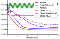
We consider detecting upright people in a multi-camera settings, using the Probabilistic Occupancy Map approach (POM, [12]), that relies on a random field with high-order repulsive potentials, which models background subtraction signal given the presences of people in the environment. We evaluate it on the ISSIA [9] dataset, which contains 3000 frames of a football game, captured by 6 cameras located on two sides of the field. The original work [12] does not explicitly mention it, but the publicly available implementation uses the ADHOC damping method. We implement all our methods and remaining baselines directly in this code of [12].

Semantic Segmentation

We consider semantic segmentation on PASCAL VOC 2012 dataset [11], which defines 20 object classes and 1 backround class. We based our evaluation on DeepLab-CRF model [8], which is currently one of the best-performing methods. This model uses CNNs to obtain unary potentials, and then employs densecrf of [22] with dense pairwise potentials. However, this basic CRF model does not contain any strong repulsive terms, and thus we expect densecrf’s standard inference, FULL-PARALLEL, to work well. To improve performance, we additionally introduced co-occurrence potentials [30], which, as we will show, violate the conditions assumed in densecrf, but can still be successfully handled by our method. Intuitively, these co-occurrence terms put priors on the sets of classes that can appear together. We made minor modifications of densecrf to support both our inference and co-occurrence potentials.

4.3 Comparative Results

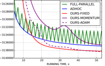
In order to understand how the methods behave in practical settings, when the available computational time is limited, we evaluate all methods for several computational budgets. The shortest budget corresponds to the early-stopping scenario after few iterations, the longest one roughly models the time until convergence, and the middle one is around 20-30% of the longest.

Benchmarks

	DBN			GRID			SEG
method	0.05s	0.30s	1.00s	0.05s	0.30s	1.00s	0.05s	0.30s	1.00s
SWEEP	-112.94	-2088.07	-2138.13	-5540.59	-16675.55	-18592.26	78.81	75.50	75.50
FULL-PARALLEL	-1952.52	-1951.54	-1942.86	-2564.39	-2777.33	-2439.08	75.66	75.66	75.66
ADHOC	-2047.31	-2047.31	-2047.31	-18345.42	-18348.80	-18349.03	76.10	75.66	75.66
OURS-FIXED	-2081.91	-2081.91	-2081.91	-18213.81	-18219.42	-18219.45	77.17	75.61	75.61
OURS-ADAPTIVE	-2125.48	-2130.61	-2130.61	-18245.93	-18252.48	-18252.48	77.68	75.64	75.61
OURS-MOMENTUM	-2260.98	-2362.14	-2374.51	-18143.48	-19074.45	-19184.37	74.35	73.75	73.75
OURS-ADAM	-2107.98	-2107.93	-2107.93	-18617.06	-18732.59	-18740.36	72.37	72.32	72.32

Table 1: Results for KL minimization for three benchmark datasets [13]: DBN (deep belief networks), GRID (two-dimensional grids), SEG (binary segmentation). All the numbers are KL divergence (lower is better) averaged over the instances.

DBN(0.05s)	DBN(0.3s)	GRID(0.05s)	GRID(0.3s)	SEG(0.05s)	SEG(0.3s)

Figure 2: Insensitivity of OURS-FIXED (red) and OURS-ADAPTIVE (dashed red) vs ADHOC (blue) to the damping parameter $\eta=\frac{1}{1+d}$. We report KL-divergence (lower is better) vs the value of the parameter, both in log-space.

(a) Characters Inpainting	(b) People Detection	(c) Semantic Segmentation

Figure 3: Convergence results. (a) OURS-ADAM and OURS-MOMENTUM converge very fast to a much better minima. (b) OURS-FIXED outperforms ADHOC both in terms of speed of convergence and the value of the objective. (c) OURS-ADAM and OURS-FIXED show the best performance. The former converges a bit slower, but in the end provide slightly better minima. ADHOC for this dataset converges rather fast, but fails to find a better optima.

	0.05s		0.3s		3s
method	KL	PA	KL	PA	KL	PA
SWEEP	-6342.56	54.57	-25233.54	58.38	-49519.33	62.50
FULL-PARALLEL	-49516.98	60.99	-49519.27	62.00	-49519.33	62.05
ADHOC	-49514.27	61.46	-49520.09	62.15	-49520.20	62.17
OURS-FIXED	-49505.59	60.99	-49520.33	62.26	-49521.71	62.35
OURS-ADAPTIVE	-49503.43	60.93	-49520.14	62.32	-49522.49	62.60
OURS-MOMENTUM	-49513.57	63.69	-49536.67	65.26	-49540.76	65.95
OURS-ADAM	-49516.02	65.36	-49538.84	67.03	-49544.58	67.12

Table 2: Results for characters inpainting problem [25] based on DTFs. PA is the pixel accuracy for the occluded region (bigger is better). Our methods outperform the baselines by a margin of 3-5%. Since FULL-PARALLEL is not damped, it gets to low KL-divergence value quickly, however the actual solution is significantly worse.

	0.5s		1.3s		5s
method	KL	MODA	KL	MODA	KL	MODA
SWEEP	1865.43	0.630	1795.66	0.656	1795.60	0.656
FULL-PARALLEL	2573.79	0.000	2573.79	0.000	8500.90	0.030
ADHOC	2573.79	0.308	1760.02	0.781	1753.71	0.829
OURS-FIXED	1783.63	0.626	1754.55	0.802	1753.63	0.829
OURS-MOMENTUM	1931.36	0.040	1797.19	0.650	1753.83	0.826
OURS-ADAM	2008.52	0.021	1813.66	0.501	1754.52	0.824

Table 3: Results for people detection task [9] based on POM [12]. OURS-FIXED outperforms the baselines and adaptive methods. This means that this problem does not require more sophisticated parameter exploration techniques.

	5s		15s		50s
method	KL	I/U	KL	I/U	KL	I/U
FULL-PARALLEL [o]	$-$	67.18	$-$	67.70	$-$	68.00
OURS-ADAM [o]	$-$	66.45	$-$	67.50	$-$	68.07
FULL-PARALLEL	-3129799	67.21	-3134437	67.72	-3133010	68.01
ADHOC	-3129469	67.19	-3134557	67.73	-3136865	68.04
OURS-FIXED	-3100079	67.76	-3135225	68.18	-3138206	68.44
OURS-MOMENTUM	-3060405	66.20	-3128121	67.39	-3136543	68.18
OURS-ADAM	-3091787	67.08	-3131624	68.02	-3138335	68.47

Table 4: Results for semantic segmentation problem [11] based on DeepLab-CRF [8]. For all the budgets, our method obtains better segmentation accuracy. Again, FULL-PARALLEL obtains lower KL faster, with a price of reduced performance. On the top, we provide results for the original DeepLab-CRF model without co-occurrence potentials (denoted by [o]), for which the KL divergence has therefore a different meaning and is not shown.

Quantitative results are given in Table 1. Our methods systematically outperform the ADHOC damping method. The SWEEP method usually provides good performance, but is generally slow due to its sequential nature.

Fig. 2 shows that our methods are less sensitive to damping parameter changes than ADHOC. In Fig. 2, the vertical orange lines corresponds to the choice of the damping parameter according to $d=L$, which can be computed directly by the power-method. Interstingly, for the GRID dataset, which includes strong repulsive potentials, algorithms do not produce reasonable results when no damping is applied. On the other hand, for the segmentation task, SEG, all the algorithms work well even without damping, in accordance with the results of [22] or Section 3.2.

Characters Inpainting

Quantitative results in terms of average pixel accuracies and KL-divergences are given in Table 4 and Fig. 3 (a). Our method, especially when used with more advanced gradient descent schemes, outperforms all the baselines. SWEEP shows relatively good performance, but does not scale as well in terms of the running time. See the bottom row of Fig. 1 for an example of a result.

People Detection

Quantitative results, presented in Table 4 and Fig. 3 (b), demonstrate that our method with a fixed step size, OURS-FIXED, brings both faster convergence and better performance. Thanks to our optimization scheme, the time required to get a Multiple Object Detection Accuracy(MODA, [4]) within 3% of the value at convergence is reduced by a factor of two. This can be of big practical importance for surveillance applications of the algorithm [3, 2], in which it is required to run in real-time. SWEEP exhibits much worse performance than our parallel method because of its greedy behaviour.

Semantic Segmentation

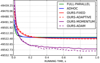
Quantitative results are presented in Table 4 and Fig. 3 (c). We observe that a similar oscillation issue as noted by [30] starts happening when the FULL-PARALLEL method is used in conjunction with co-ocurrence potentials, producing even worse results than without those. Using our convergent inference method fixes oscillations and provides an improvement of 0.5% in the average Intersection over Union measure (I/U) compared to the basic method without co-occurrence. This is a significant improvement that would be sufficient to increase the position of an algorithm by 2 or 3 places in the official ranking [11]. What it represents is a big improvement in performance, as the ones shown in Fig 1, for at least 30-40 images out of total 1449. Note also, that we obtain this improvement with minimal changes in the original code. By contrast, authors [8] get similar or smaller improvements by significantly augmenting the training set or by exploiting multi-scale features, which leads to additional computational burden.

5 Discussion and Future Work

We have presented a principled and efficient way to do parallel mean-field inference in discrete random fields. We have demonstrated that proximal gradient descent is a powerful theoretical framework for mean-field inference, which unifies and sheds light on previous approaches. Moreover, it naturally allows to incorporate existing adaptive gradient descent techniques, such as ADAM, to mean-field methods. As shown in our experiments, it often brings dramatic improvements in performance. Additionally, we have demonstrated, that our approach is less sensitive to the choice of parameters, which makes it easier to use in practice.

Importantly, our method brings considerable improvements in terms of performance on three realistic Computer Vision problems, while being very easy to implement.

Our method makes it possible to use mean-field inference with a much wider range of potential functions, which was previously unachievable due to the lack of convergent optimization. Thus, there is a large amount of possible future applications of our approach, especially in the tasks where higher-order and repulsive potentials can bring additional benefits, not only in segmentation, but also in object detection and localization.

References

- [1] S.-I. Amari. Natural Gradient Works Efficiently in Learning. Neural computation, 10(2):251–276, 1998.
- [2] T. Bagautdinov, P. Fua, and F. Fleuret. Probability Occupancy Maps for Occluded Depth Images. In Conference on Computer Vision and Pattern Recognition, 2015.
- [3] H. BenShitrit, J. Berclaz, F. Fleuret, and P. Fua. Multi-Commodity Network Flow for Tracking Multiple People. IEEE Transactions on Pattern Analysis and Machine Intelligence, 36(8):1614–1627, 2014.
- [4] K. Bernardin and R. Stiefelhagen. Evaluating Multiple Object Tracking Performance: the Clear Mot Metrics. EURASIP Journal on Image and Video Processing, 2008, 2008.
- [5] C. Bishop. Pattern Recognition and Machine Learning. Springer, 2006.
- [6] Y. Boykov, O. Veksler, and R. Zabih. Fast approximate energy minimization via graph cuts. Pattern Analysis and Machine Intelligence, IEEE Transactions on, 23(11):1222–1239, 2001.
- [7] N. Campbell, K. Subr, and J. Kautz. Fully-connected crfs with non-parametric pairwise potential. In Conference on Computer Vision and Pattern Recognition, pages 1658–1665, 2013.
- [8] L.-C. Chen, G. Papandreou, I. Kokkinos, K. Murphy, and A. L. Yuille. Semantic image segmentation with deep convolutional nets and fully connected crfs. In ICLR, 2015.
- [9] T. D’Orazio, M. Leo, N. Mosca, P. Spagnolo, and P. L. Mazzeo. A Semi-Automatic System for Ground Truth Generation of Soccer Video Sequences. In International Conference on Advanced Video and Signal Based Surveillance, pages 559–564, 2009.
- [10] J. C. Duchi, S. Shalev-Shwartz, Y. Singer, and A. Tewari. Composite objective mirror descent. In COLT, pages 14–26. Citeseer, 2010.
- [11] M. Everingham, L. Van Gool, C. K. I. Williams, J. Winn, and A. Zisserman. The PASCAL Visual Object Classes Challenge 2012 (VOC2012) Results. http://www.pascal-network.org/challenges/VOC/voc2012/workshop/index.html.
- [12] F. Fleuret, J. Berclaz, R. Lengagne, and P. Fua. Multi-Camera People Tracking with a Probabilistic Occupancy Map. IEEE Transactions on Pattern Analysis and Machine Intelligence, 30(2):267–282, February 2008.
- [13] R. Frostig, S. Wang, P. Liang, and C. Manning. Simple MAP Inference via Low-Rank Relaxations. In Advances in Neural Information Processing Systems, pages 3077–3085, 2014.
- [14] A. E. Gelfand and A. F. Smith. Sampling-based approaches to calculating marginal densities. Journal of the American statistical association, 85(410):398–409, 1990.
- [15] L. Gorelick, Y. Boykov, O. Veksler, I. Ben Ayed, and A. Delong. Submodularization for binary pairwise energies. In Computer Vision and Pattern Recognition (CVPR), 2014 IEEE Conference on, pages 1154–1161. IEEE, 2014.
- [16] M. Hoffman, D. Blei, C. Wang, and J. Paisley. Stochastic Variational Inference. Journal of Machine Learning Research, 14(1):1303–1347, May 2013.
- [17] M. E. Khan, P. Baqué, F. Fleuret, and P. Fua. Kullback-Leibler Proximal Variational Inference. In NIPS, 2015.
- [18] D. P. Kingma and J. Ba. Adam: A method for stochastic optimization. CoRR, abs/1412.6980, 2014.
- [19] D. Koller and N. Friedman. Probabilistc Graphical Models. The MIT Press, 2009.
- [20] V. Kolmogorov. A new look at reweighted message passing. Pattern Analysis and Machine Intelligence, IEEE Transactions on, 37(5):919–930, 2015.
- [21] P. Krähenbühl and V. Koltun. Efficient Inference in Fully Connected CRFs with Gaussian Edge Potentials. In Advances in Neural Information Processing Systems, 2011.
- [22] P. Krähenbühl and V. Koltun. Parameter Learning and Convergent Inference for Dense Random Fields. In International Conference on Machine Learning, pages 513–521, 2013.
- [23] T. P. Minka. Expectation propagation for approximate bayesian inference. In Proceedings of the Seventeenth conference on Uncertainty in artificial intelligence, pages 362–369. Morgan Kaufmann Publishers Inc., 2001.
- [24] K. Murphy, Y. Weiss, and M. Jordan. Loopy Belief Propagation for Approximate Inference: An Empirical Study. In Onference on Uncertainty in Artificial Intelligence, pages 467–475, 1999.
- [25] S. Nowozin, C. Rother, S. Bagon, T. Sharp, B. Yao, and P. Kholi. Decision Tree Fields. In International Conference on Computer Vision, November 2011.
- [26] B. T. Polyak. Some methods of speeding up the convergence of iteration methods. USSR Computational Mathematics and Mathematical Physics, 4(5):1–17, 1964.
- [27] M. Saito, T. Okatani, and K. Deguchi. Application of the Mean Field Methods to MRF Optimization in Computer Vision. In Conference on Computer Vision and Pattern Recognition, June 2012.
- [28] X. Sun, M. Christoudias, V. Lepetit, and P. Fua. Real-Time Landing Place Assessment in Man-Made Environments. Machine Vision and Applications, 2013.
- [29] M. Teboulle. Entropic proximal mappings with applications to nonlinear programming. Mathematics of Operations Research, 17(3):pp. 670–690, 1992.
- [30] V. Vineet, J. Warrell, and P. Torr. Filter-Based Mean-Field Inference for Random Fields with Higher-Order Terms and Product Label-Spaces. International Journal of Computer Vision, 110(3):290–307, 2014.
- [31] M. Wainwright and M. Jordan. Graphical Models, Exponential Families, and Variational Inference. Foundations and Trends in Machine Learning, 1(1-2):1–305, Jan. 2008.
- [32] J. Winn and C. Bishop. Variational Message Passing. In Journal of Machine Learning Research, pages 661–694, 2005.
- [33] S. Zheng, S. Jayasumana, B. Romera-Paredes, V. Vineet, Z. Su, D. Du, C. Huang, and P. Torr. Conditional random fields as recurrent neural networks. In International Conference on Computer Vision (ICCV), 2015.