Spectral Eclipse Timing

Abstract

We utilize multi-dimensional simulations of varying equatorial jet strength to predict wavelength dependent variations in the eclipse times of gas-giant planets. A displaced hot-spot introduces an asymmetry in the secondary eclipse light curve that manifests itself as a measured offset in the timing of the center of eclipse. A multi-wavelength observation of secondary eclipse, one probing the timing of barycentric eclipse at short wavelengths and another probing at longer wavelengths, will reveal the longitudinal displacement of the hot-spot and break the degeneracy between this effect and that associated with the asymmetry due to an eccentric orbit. The effect of time offsets was first explored in the IRAC wavebands by Williams et al. (2006). Here we improve upon their methodology, extend to a broad ranges of wavelengths, and demonstrate our technique on a series of multi-dimensional radiative-hydrodynamical simulations of HD $209458$b with varying equatorial jet strength and hot-spot displacement. Simulations with the largest hot-spot displacement result in timing offsets of up to $100$ seconds in the infrared. Though we utilize a particular radiative hydrodynamical model to demonstrate this effect, the technique is model independent. This technique should allow a much larger survey of hot-spot displacements with JWST then currently accessible with time-intensive phase curves, hopefully shedding light on the physical mechanisms associated with thermal energy advection in irradiated gas-giants.

1. Introduction

Highly irradiated, presumably tidally locked, short-period gas-giant planets have provided invaluable information in our quest to understand the formation and evolution of exoplanets. Given their proclivity to transit and their favorable size relative to their host stars, a wealth of information has been extracted observationally and they will likely remain the best characterized of all exoplanets. However, they are significantly different than our own gas-giant planets. Most striking is the influence of the incident stellar energy, which provides a luminosity $\sim 10^{5}$ times higher then the internal luminosity of the planet. The role of this incident energy in influencing the planet’s evolution and shaping the observable features remains an outstanding question, crucial for interpreting and understanding the wealth of observations.

A number of groups are studying the atmospheric behavior of gas-giant planets utilizing multi-dimensional radiative-hydrodynamical models. For a non-exhaustive list of groups and techniques utilized see Dobbs-Dixon & Agol (2013); Heng & Showman (2014). Though the details vary between models, there is a general consensus that highly irradiated, tidally locked gas-giant planets form broad, supersonic, super-rotating, equatorial jets. These equatorial jets account for a vast majority of the dynamical energy transport, and are responsible for differences between radiative-only calculations and the fluxes actually observed.

In a very general sense, the efficiency of energy transport via a jet can be described by two parameters: the radiative time-scale (how long it takes to cool) and the dynamical time-scale (how long it takes fluid to move from day to night). We expect these two time-scales to be comparable. For example, consider a highly irradiated planet where the radiative time-scale is significantly shorter then the dynamical time-scale; the gas would cool very efficiently as it travels from day to night. However, the lack of thermal energy transport to the night-side implies the day-night pressure differential (the primary driving force for the winds) would be extremely large. This would shorten the dynamical time-scale, bringing it closer into line with the radiative time-scale.

As the number of short-period gas-giant planets discovered to be transiting their host stars continues to increase, we can begin to make detailed comparisons to predictions from multi-dimensional radiative-hydrodynamical models. One of the most dramatic set of observations that demonstrates the importance of dynamics are full or partial phase curves of short-period planets in the infrared. Though necessarily hemispherically averaged, it is possible to extract the longitudinal dependence of the thermal emission across the surface of the planet (Cowan & Agol, 2008). Differences between observed phase curves and those predicted from a radiative-equilibrium calculation can be attributed to the transport of thermal energy via vigorous atmospheric dynamics. Given the current accuracy of observations, the most telling aspects of a phase curve are the location of the maximum and minimum flux, and the day-night temperature differential.

The most accurate phase curve to date is an $8\micron$ observation of HD $189733$b by Knutson et al. (2007, 2009); Knutson et al. (2012). They find the peak in the thermal emission from the planet occurs $2.3$ hours before secondary eclipse, indicative of downwind advection by a strong equatorial jet, and day-night temperature differential of $\sim 240$K. However, offsets and day-night temperature contrasts are not universal. Cowan et al. (2007) monitored the phase-variations of three planets at $3.6$ and $4.5$ and $8\micron$, finding that only HD $179949$b exhibited any variation in phase, while observations of HD $209458$b (Zellem et al., 2014) and $51$-Peg showed no variation indicating extremely efficient energy redistribution. It is important to note that these phase curves are relatively sparsely populated and consist of non-consecutive observations. The first phase curve of the non-transiting planet $\nu$-Andromeda (Harrington et al., 2006; Crossfield et al., 2010) suggests a temperature differential of over $900$K and a hot-spot offset of $\sim 80^{\circ}$.

In this paper we focus on the location of the hot-spot. We currently do not understand why some planets exhibit hot-spot offsets while others do not. As discussed above, this should ultimately be related to variations in dynamical and radiative efficiencies. However, this simple interpretation may not be sufficient. For example, one might expect a large hot-spot offset to be correlated to a small temperature differential. This picture seems to work for HD $189733$b with its moderate hot-spot offset and several hundred degree temperature differential. However, the hot-spot on $\nu$-Andromeda is extremely large and the temperature differential is huge. In hopes of understanding the importance of composition, incident flux, etc. in determining the efficiency of heat transfer by the atmosphere, significantly more data would be extremely helpful. Unfortunately, full or half orbit phase curves use significant telescope time, and surveying many systems is difficult. Here we explore a technique for extracting the longitudinal offset of the hot-spot via a single, multi-wavelength observation of secondary eclipse utilizing variations in the time of secondary eclipse. We illustrate the technique by using multi-dimensional radiative hydrodynamical models of the giant planet HD $209458$b to predict the timing offsets as a function of wavelength. In Section (2) we briefly discuss the multi-dimensional models, explain how to extract emission maps from the simulations, and discuss the technique for calculating the wavelength-dependent timing offsets. In Section (3) we present our predictions for HD $209458$b, and discuss the correlation between timing differences and hot-spot offsets. A variant of this technique was first proposed by Williams et al. (2006), who used the simulations of Cooper & Showman (2005) to predict eclipse-timing offsets (they refer to these as uniform time offsets) in Spitzer’s four IRAC bandpasses. We compare our methods and results to theirs in Section (3.1). Finally, we discuss the feasibility of such a measurement given current and future instrumental limitations in Section (3.2). Section (4) concludes with a general discussion of our results.

2. Calculating Observables from 3D Models

To illustrate the concept of variations in transit-timing due to an offset hot-spot we concentrate on simulations of the transiting gas-giant planet HD $209458$b. We begin by briefly discussing our simulations, explain the technique for extracting observable emission maps, and finally the technique used to calculate variations in transit-timing.

2.1. Dynamical Simulations

In Dobbs-Dixon et al. (2012) we performed extensive simulations of HD $209458$b utilizing our multi-dimensional radiative-hydrodynamical model. The model solves the fully compressible Navier-Stokes equations throughout the entire atmosphere from pressures of $10^{-6}$ to $500$ bars. The dynamical equations are coupled to a wavelength dependent stellar energy deposition, radiative-transfer via flux-limited diffusion, and a two-temperature energy equation. See Dobbs-Dixon et al. (2012) for a discussion on solution techniques, resolution information, and parameter choices. We compared our results to observed transit spectra, finding excellent agreement, and predicted wavelength-dependent timing variations in center of primary transit. Note that the variations in primary transit timing we discuss in Dobbs-Dixon et al. (2012) differ from what we present here. Though both related to dynamics, deviations during primary transit are due to differences in the scale-height of the eastern and western terminators, while timing variations of the secondary eclipse discussed here are primarily due to variations in hot-spot location.

To explore the efficiency of the equatorial jet in redistributing energy throughout the atmosphere, Dobbs-Dixon et al. (2012) performed a number of simulations with viscosity varying from $10^{8}$ to $10^{12}\,cm^{2}/s$. Viscosity serves as a mechanism to self-consistently convert the kinetic energy of the flow back into thermal energy and is meant to encapsulate the effect of shocks, instabilities, or other sources of un-resolved drag on the atmospheric flow. Large viscosities resulted in slow, sub-sonic flows, no jet formation, and large day-night temperature differentials. The atmospheric dynamics in these simulations did little to change the radiative temperature distribution and the hottest point on the planet remained near the sub-stellar point. However, as we decreased the viscosity, we found that a super-rotating, supersonic, equatorial jets formed that were able to efficiently transport energy to the night-side while simultaneously advecting the hot-spot downwind, east of the sub-stellar point. The smaller the viscosity, the larger the offset. Figure (3) of Dobbs-Dixon et al. (2012) shows the temperature and zonal velocity distribution at the photosphere of the planet for a range of viscosities. Although we utilize these simulations to illustrate this phenomena, we emphasize that the techniques we present are model independent and can be applied to any observation of secondary eclipse.

2.2. Observables

Multi-dimensional radiative-hydrodynamical calculations provide us with a three-dimensional distribution of temperature and density throughout the atmosphere that we can utilize to explore observational phenomena. Given temperature and density, detailed gas opacities from Sharp & Burrows (2007) allow us to calculate wavelength-dependent emission and absorption spectra, and phase curves. Of primary interest to us in this paper, are the wavelength-dependent maps of emission from the day-side of the planet. Two components contribute to this emission: thermal emission and scattered light. We discuss each in turn below.

2.2.1 Thermal Emission

To calculate the thermal emission from the day-side of the planet we integrate inwards along rays parallel to the line of sight. The positional dependent intensity required to calculate the detailed secondary eclipse light curve is given by

$$I_{emis}\left(x,y,\lambda\right)=\frac{\lambda^{2}}{c}\int_{0}^{\infty}B_{\lambda}\left(x,y,\tau\right)e^{-\tau_{\lambda}}d\tau_{\lambda}.$$ (1)

We assume the atmospheric gas emits as a Blackbody, given by

$$B_{\lambda}\left(x,y,\tau\right)=\frac{2\pi hc^{2}/\lambda^{5}}{exp\left(\frac{hc}{\lambda kT}\right)-1}.$$ (2)

The density and temperature values, used in Equation (2) and needed to calculate $\tau$ at each location, are interpolated from the values calculated in the 3D models. Finally the total apparent day-side luminosity can be obtained by integrating over the observed disk

$$L_{p}\left(\lambda\right)=\int I_{p}dA,$$ (3)

where $dA$ is the area element in the observer’s plane.

2.2.2 Scattered Light

We assume a uniform albedo and diffuse scattering for the planet. To calculate the incident stellar light scattered from the planet we first consider the specific intensity emitted in the direction of the observer. The frequency dependent intensity scattered from each longitude ($\phi$) and latitude ($\theta$) on the planet can be written as

$$I_{scat}\left(\phi,\theta,\nu\right) = A_{S}\left(\phi,\theta,\nu\right)I_{inc}cos\phi cos\theta$$

$$= \left(\frac{3}{2}\right)A_{g}\left(\phi,\theta,\nu\right)I_{inc}cos\phi cos\theta,$$

where $A_{S}$ and $A_{g}$ are the spherical and geometric albedo respectively. The scattered intensity is understood to only be relevant for the longitudes and latitudes both exposed to the stellar light, and visible to the observer during the eclipse; i.e. within $\phi,\theta=\pm\pi/2$ of the sub-stellar point $\left(\phi,\theta\right)=\left(0^{\circ},0^{\circ}\right)$. The $cos\phi cos\theta$ term accounts for the angle between the local normal and the incident stellar intensity, $I_{inc}=B_{\star}\left(\nu\right)\left(\frac{R_{\star}}{a}\right)^{2}$.

The light scattered toward the observer can be calculated by integrating Equation (2.2.2) over the entire observable hemisphere, adding a geometric term to account for the reduced area visible and the standard spherical area element. This gives the intensity scattered towards the observer,

$$I_{scat}\left(\nu\right)=R_{p}^{2}\left(\nu\right)\int\int I_{scat}\left(\phi,\theta,\nu\right)cos\phi_{obs}cos^{2}\theta_{obs}d\phi d\theta.$$ (5)

In the limit of spatially constant albedo, this can be integrated and written in the usual form as

$$I_{scat}\left(\nu\right)=R_{p}^{2}A_{g}\left(\nu\right)I_{inc}\left(\nu\right)\frac{sin\alpha+\left(\pi-\alpha\right)cos\alpha}{\pi}.$$ (6)

The final fraction is the well known Lambertian phase-function. In the following we assume a spatially constant albedo. However, theoretical calculations (Lee et al., 2015) and multiple observations (Demory et al., 2013; Esteves et al., 2014; Hu et al., 2015; Shporer & Hu, 2015) suggest that cloud coverage may not be spatially uniform. In this case, one must use Equation (5) for the scattered light contribution.

2.2.3 Calculating Timing Offsets

Utilizing the total surface brightness of the planet, we generate simulated secondary eclipse light curves by integrating over the visible portion of the planet at each time step. We used the planet radius and orbital parameters derived in Torres et al. (2008). Once wavelength dependent simulated light curves are computed, we utilize the standard observational technique to fit them using a secondary eclipse model that assumes a uniform planet surface brightness (Mandel & Agol, 2002). If the planet was in radiative equilibrium the mid-eclipse time of transit would coincide with the midpoint of barycentric secondary eclipse. Deviation in the planet’s surface brightness gives the so-called “uniform time offset” (Williams et al., 2006); this corresponds to the artificial time inferred using the wrong (i.e. uniform) planet emission model.

3. Predicted Timing Offsets

Utilizing the simulations of HD $209458$b from Dobbs-Dixon et al. (2012) and the techniques described in Section (2) we calculate the variation in the time of central eclipse. Figure (1) illustrates our results for models with varying viscosity and jet strength using the both the thermal emission and scattered light, $I_{tot}=I_{emis}+I_{scat}$. As expected, smaller viscosities and stronger equatorial jets are associated with larger timing offsets. For simulations with large hot-spot displacements we predict timing offsets of up to $96$ seconds at $2\micron$. At longer wavelengths Figure (1) shows a general trend of increasing timing offset with decreasing wavelength. This is the result of increasingly spatially inhomogeneous (patchy) emission at shorter wavelengths (see Figure 2). Due to the steep slope of the emission spectra in the Wien tail, small changes in gas temperature lead to significant changes in emission resulting in patchy emission and large timing offsets. This effect becomes more pronounced at shorter wavelengths. However the scattered light, inherently symmetric based on our assumptions, acts to damp out any timing offsets seen at even shorter wavelengths. For calculations assuming a small albedo ($0.05$) this cutoff is approximately $1\micron$, while those assuming a larger albedo ($0.35$) the cutoff wavelength is somewhat longer, at $3\micron$. Note that though we include the effects of albedo on timing predictions, we have not self-consistently modified the stellar energy deposition in the multi-dimensional simulations. All simulations assume zero albedo, while a non-zero albedo is used in post-processing the simulated atmospheres with our radiative transfer code. Thus, a small error in the temperature of the planet is made of the order $(1-A)^{1/4}$; this will affect our results quantitatively, but we expect will capture the same qualitative features as a fully self-consistent computation. The detailed features seen in all curves in Figure (1) are associated with peaks in the opacity, primarily due to water. A larger opacity implies we are probing higher in the atmosphere where the planet asymmetries are larger, while wavelengths corresponding to smaller opacities probe deeper, more symmetric regions of the atmosphere, resulting in smaller time offsets. In Table (1) we detail eclipse timing offsets averaged over J, H, K, IRAC, and proposed James Webb Space Telescope (JWST) bandpasses.

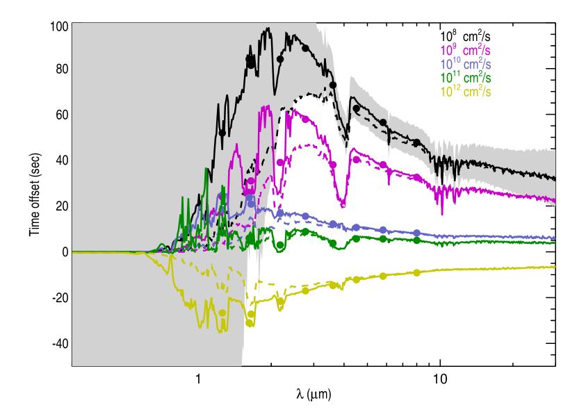
Figure 1.— Variation in the time of secondary eclipse for models of HD $209458$b with varying viscosities and jet strengths. The solid lines are calculated assuming an albedo of $0.05$ while the dashed lines assume a value of $0.35$. Solid dots show the band-averaged time offsets reported in Table (1). The shaded region shows the extent of the observational errors on the time offset for a planet with a viscosity of $10^{8}\,cm^{2}/s$ around sun-like star at $10$ parsecs viewed by JWST (See discussion in Section (3.2)).

To further illustrate the relative contributions of scattered light and thermal emission we show intensity maps from the day-side of the planet for a range of wavelengths in Figure (2). The top row shows the contribution from thermal emission, the middle from scattered light, and the bottom shows the total. Thermal emission maps are calculated using the lowest viscosity simulation ($10^{8}\,cm^{2}/s$) while scattered light maps assume an albedo of $0.05$. At $\lambda=0.7\micron$ (left column) the peak of the thermal emission exhibits a large offset, but is orders of magnitude smaller then the scattered light and is completely masked in the total emission. At $\lambda=10\micron$ (right column) the thermal emission is also offset, though not as strongly peaked, and several orders of magnitude brighter then the scattered light. The total emission is thus dominated by the thermal component. At intermediate wavelengths ($\lambda=1.3\micron$, middle column) the thermal and scattered intensities are comparable and the resulting peak of the total emission is pulled back toward the sub-stellar point.

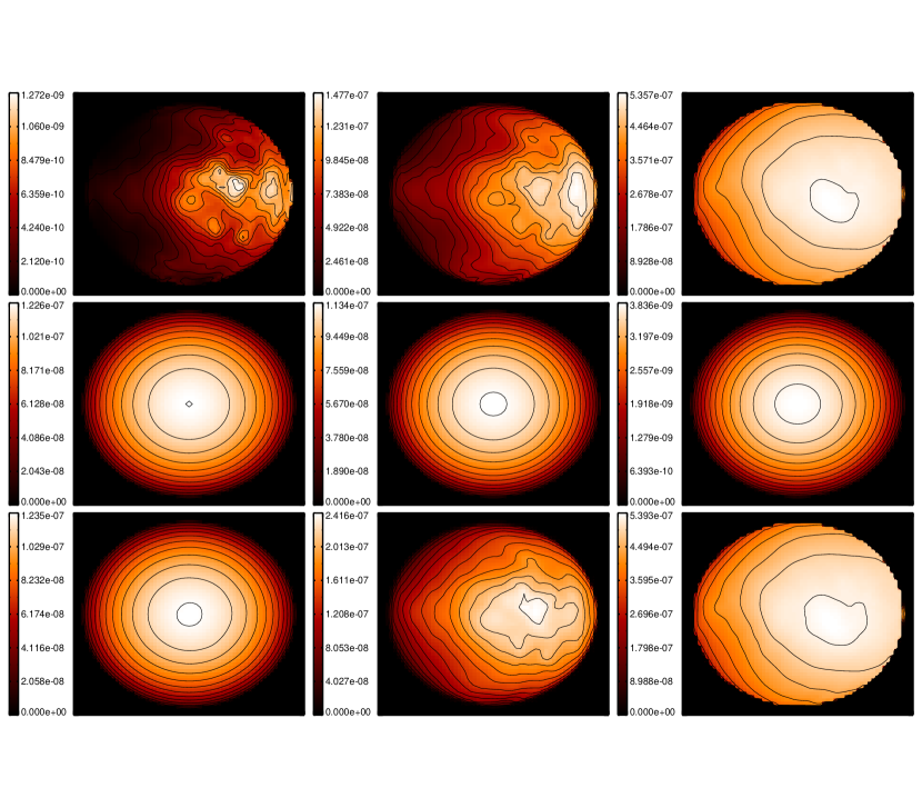
Figure 2.— The day-side intensity from thermal emission (top row), the scattered intensity (middle row), and the total intensity (bottom row) at several representative wavelengths. The first column shows the results for $\lambda=0.7\micron$, the middle column shows $\lambda=1.3\micron$, and the final column shows $\lambda=10\micron$. The sub-stellar point is located at the center of each image. Note the scale of each plot is different.

Band	$10^{8}$	$10^{9}$	$10^{10}$	$10^{11}$	$10^{12}$	Williams
J	51.9	24.0	18.4	8.4	-26.7	-
H	81.4	31.0	20.8	4.8	-27.2	-
Ks	84.1	39.0	16.7	3.0	-21.6	-
F162M	84.2	25.9	23.7	6.0	-31.0	-
F277W	88.9	57.9	15.5	8.8	-17.0	-
IRAC1	72.8	39.0	12.1	3.7	-14.7	53.0
IRAC2	62.6	40.2	10.6	5.7	-12.2	49.5
IRAC3	56.5	38.0	9.5	5.7	-10.6	44.0
IRAC4	47.8	32.5	8.2	5.0	-9.2	37.5

Table 1Band averaged eclipse time offsets in seconds for several representative bandpasses (including the proposed F162M and F277W JWST filters) for models with viscosities ranging from $10^{8}$ to $10^{12}\,cm^{2}/s$. The final column lists results from our $\nu=10^{8}\,cm^{2}/s$ simulation using the methodology of Williams et al. (2006).

3.1. Comparison with Williams et al. (2006)

Studying the effect of an offset hot-spot on the time of center of eclipse was first proposed by Williams et al. (2006). Referring to this phenomena as a uniform time offset, they predicted signals of $86$, $77$, $67$, and $57$ seconds for the IRAC wavebands $1-4$ and explored the probability of such a detection. Our current predictions differ from Williams et al. (2006) in three important ways: the underlying radiative-hydrodynamical method and solution, the method for calculating intensity maps, and the wavelength range explored. Though the last point is most crucial, we explore each below in turn.

The first difference between the predictions of Williams et al. (2006) and that presented here is that the underlying multidimensional radiative-hydrodynamical model used to generate predictions is different. They utilize results from the model of Cooper & Showman (2005), which is a general circulation model (GCM) solving the primitive equations coupled to a simplified Newtonian cooling scheme. Cooper & Showman (2005) predicts an hot-spot offset of $60^{\circ}$ in longitude at the wavelength-averaged photosphere. Our simulations, described in detail in Section (2.1) utilizes a significantly different numerical code and can produce a range of hot-spot offsets associated with varying viscosity.

The second difference is the manner of producing the intensity map. In Williams et al. (2006) they utilized the calculations of Fortney et al. (2005) to identify approximate pressures that correspond to the photosphere of the planet when viewed in each of the four IRAC bandpasses ($105$, $50$, $35$, and $24$ mbar for IRAC1 through IRAC4). They then identify the corresponding temperature at each latitude/longitude, assume that each patch of the planet emits as a blackbody, and sum up all the contributions to get the total thermal emission. In this work, as described in Section (2.2), we integrate the emission contributions along the line of sight, thus accounting for the fact that the path of the light is increasingly non-radial as you move toward the limb of the planet. The emitted flux does not simply come from a single pressure, but rather a range around the $\tau=1$ surface associated with the contribution function (Chamberlain & Hunten, 1987; Knutson et al., 2009) as you integrate along the path. We additionally include the important contribution from scattered light. Though not relevant at the longer wavelength IRAC bands, it is imperative to include scattered light at wavelengths near and below $\sim 1\,\mu m$. The initial assumption in the community at large was that optical secondary eclipses would never be observable (likely explaining why Williams did not include it). However, particularly for very hot planets such as Wasp-12b (Hebb et al., 2009), we find that including scattered light is necessary below $\sim 1\,\mu m$. The final difference is that we explore the eclipse timing offsets over a much wider range of wavelengths. Though this may appear trivial, we suggest that the actual measurement of this effect will require a differential measurement between two or more wavelengths. The barycentric eclipse cannot be determined from radial velocities to sufficient accuracy to determine the offset from a single wavelength. By expanding our wavelength coverage, observers may choose two wavelength regions with maximal timing differentials, yielding a potentially observable signature.

To test the importance of the technique used when producing an emission map of the planet, we produced IRAC light curves utilizing the blackbody radiation associated with the constant pressure surfaces of $105$, $50$, $35$, and $24$ mbar (following Williams et al. (2006) technique) utilizing our lowest viscosity ($10^{8}\,cm^{2}/s$) simulation. These pressures are taken from Fortney et al. (2005) as the mean pressures associated with the IRAC photospheres. Predictions associated with constant pressure surfaces are listed in the last column of Table (1) and should be compared to values in the first column. Though there is reasonably good agreement, our non-radial ray-tracing method of calculating thermal emission maps yields timing offsets that are systematically $10-20$ seconds larger then when utilizing the constant pressure method. This can be understood by considering where in the planet the observed flux is actually coming from. As you move away from the sub-observer point the contribution function (i.e. the region where photons originate) moves to lower and lower pressures. Put another way, when integrating a photons path backwards along the correct slant-geometry (as opposed to a path normal to the planet’s surface) you will reach the $\tau\left(\lambda\right)=1$ surface much more rapidly. Therefore, as you near the limb of the planet you are looking further up in the atmosphere where dynamical redistribution has an increasingly larger roll. We did not extend the constant-pressure analysis to shorter wavelengths as short-ward of $\sim 1\,\mu m$ the methods disagree substantially due to our added contribution of scattered light. It is important to emphasize that we cannot directly compare our results to those in Williams et al. (2006) as the underlying radiative-hydrodynamical models and thus the pressure-temperature distributions are different. Our calculations of constant pressure maps are derived from the simulations from Dobbs-Dixon et al. (2012).

3.2. Observational Feasibility

To explore the feasibility of measuring a secondary eclipse time offset due to the effects of atmospheric circulation we use numerical eclipse curves to calculate the photometric precision needed to achieve a given timing error. We construct two eclipse curves using the Mandel & Agol (2002) method, normalizing them to unity during eclipse (star only). One eclipse curve represents the barycentric eclipse and the other is shifted in time by $t$ seconds. We subtract these two eclipse curves, and calculate the standard deviation of the photometric difference. That standard deviation represents the photometric error level necessary to detect a shift of $t$ seconds, to $1-\sigma$ precision. We checked our calculation by comparing to the analytic formulae given by Carter et al. (2008), (their Eq. 23) finding agreement to about 3-percent. That level of agreement is consistent with the difference between our adopted eclipse curve shape Mandel & Agol (2002), and the trapezoidal shape illustrated in Figure 1 of Carter et al. (2008).

To calculate the observed photometric error level in comparison to the required error level defined above, we assumed that Poisson-counting noise dominates the photometric uncertainties. Indeed, observations with Spitzer have achieved close to shot-noise precision (Deming et al., 2014, e.g.). We used ATLAS stellar models (Castelli & Kurucz, 2003) in order to calculate the photon flux at JWST, and we adopted a telescope area of $25m^{2}$, a throughput (electrons out divided by photons in) of $20\%$, and a filter bandwidth of $20\%$.

In Figure (3) we show the S/N for the timing offset itself, as a function of wavelength, based on the modeled timing offsets from Figure (1), for a planet eclipsed by a Sun-like star at $20$ parsecs. The shape of this curve is a confluence of the number of photons from the planet (as per above) and the size of the timing offset. Values of timing S/N peak at $8.4$ at $5\micron$, feasibly detectable by JWST, particularly when combining multiple observations. We show the expected errors associated with this S/N in Figure (1) as a shaded region for the model with a viscosity of $10^{8}\,cm^{2}/s$. Though the errors are enormous at wavelengths less than approximately $2\micron$ (primarily due to a lack of photons) they are reasonable at longer wavelengths. Note that the curve in Figure (1) is a theoretical prediction, thus independent of observational resolution. Actual observations will result in substantially lower resolution. Once a particular observation has been made, the theoretical data can be appropriately binned for comparison.

Figure 3.— The signal-to-noise as a function of wavelength for detection of the dynamically induced timing offsets for a short period planet around a sun-like star at $20$ parsecs assuming a $20\%$ throughput on JWST and a $20\%$ bandpass. Timing offsets are taken from Figure(1) for the lowest viscosity simulation and assume an albedo of $0.05$.

4. Conclusions

In this paper we propose a method to determine the horizontal displacement of the hot-spot on a tidally locked, highly irradiated, gas-giant planet. A hot-spot displaced from the sub-stellar point will introduce an asymmetry in the secondary eclipse light-curve that, when fit utilizing a model that assumes a symmetric planet will manifest itself as a timing offset of the calculated center of eclipse. In principle, this measurement could be done utilizing a single multi-wavelength observation of secondary eclipse. It is crucial to observe the eclipse in multiple wavelengths to compare calculated timing offsets to break the degeneracy associated with an eccentric orbit, as the predicted center of barycentric transit derived from radial velocity curves is not known to sufficient accuracy.

Though the method proposed in this paper is model independent we utilized radiative-hydrodynamical simulations from Dobbs-Dixon et al. (2012) of HD $209458$b to illustrate this method further and predict timing offsets. Simulations develop super-rotating equatorial jets that redistribute energy from day to night and displace the hot-spot from the sub-stellar point. Dobbs-Dixon et al. (2012) ran simulations for a range of viscosities, resulting in varying jet strengths and advective efficiencies. The hot-spots in simulations that develop little or no circumplanetary jet remain near the sub-stellar point, resulting in very little predicted time offset. Conversely, in simulations with strong, supersonic equatorial jets, the hot-spot is significantly displaced and results in timing offsets up to $\sim 100$ seconds at $2\micron$.

The concept of an offset hot-spot inducing a shift in the time of eclipse was first proposed by Williams et al. (2006). In this paper we have built upon their work in four important ways: improving the underlying radiative-hydrodynamical models, modifying the method of producing thermal emission maps, accounting for the scattered light contribution, and extending the calculation to a large wavelength range. The extension of the technique to multi-wavelength is perhaps the most crucial. When viewed in a single channel the effects that Williams et al. (2006) proposed can be interpreted as either an eccentric orbit or non-uniform planetary emission; by itself a single measurement is not conclusive. A timing differential between two or more wavebands will break the degeneracy between the eccentric and asymmetric interpretations.

There have been a number of attempts to measure the time offsets for planets at multiple wavelengths, though not necessarily simultaneous. Observations of HD $209458$b by Knutson et al. (2008) in all four Spitzer-IRAC wavebands suggests time offsets of up to $-12.6\,\pm\,3.5$ minutes for the $4.5\micron$ channel and $2.0\,\pm\,3.1$ for the $8\micron$ channel. However, our models predict a maximum differential between these wavebands of only $14.8$ seconds, so the observed $14.6\,\pm\,4.7$ minute differential is significantly larger. Measurements of time offsets for HD $209458$b by Crossfield et al. (2012) in the $24\micron$ MIPS bandpass suggest a $32\,\pm\,129$ second offset, more in line with our predictions. Re-examination of the data for HD $209458$b by Diamond-Lowe et al. (2014) suggests that the observational technique used previously resulted in much larger errors then originally quoted. Similarly, IRAC observations of of HD $189733$b utilizing a technique similar to Knutson et al. (2008) suggested differential timing offsets on the order of minutes, reaching $5.6\,\pm\,0.8$ minutes in the $3.6\micron$ channel (Charbonneau et al., 2008). However, Agol et al. (2010) used a combination of $14$ eclipses of HD $189733$b at $8\micron$ to derive a $38\,\pm\,11$ second unaccounted for shift in the center of eclipse that they attribute to an offset hot-spot. Though only measured in one waveband, this measurement is much more in line with our predictions from models with a viscosity of $10^{8}\,cm^{2}/s$. With these varying differential measurements and the associated uncertainty in observing strategies, additional observations exploring the multiwavelength timing offsets are necessary.

Ultimately, the method have described is a fairly easy way to extract information on the dynamically induced shift in the hottest point on the exoplanet. A multiwavelength observation with an instrument such as NIRSpec on JWST will allow us to differentiate between models with varying jet speed, giving us a hint of the underlying physical phenomena operating in the atmosphere. There are however, more detailed approaches that utilize the shape of the secondary eclipse to ’map’ the disk of the planet (Rauscher et al., 2007; Majeau et al., 2012; de Wit et al., 2012). The measurement described in this paper is complementary to these more detailed approaches; if measurements of time offsets indicates a significant wavelength dependent variation, one can attempt a secondary eclipse map if the S/N warrants it.

In conclusion, the location of the hot-spot is one of the most striking examples of the importance of dynamics in the atmospheres of irradiated planets. The precise location will offer clues to the interplay between the radiative and dynamical processes. Determining the strength of the offset across a diverse family of planets should help us to understand the physical phenomena involved. Observations of full or half orbit phase curves of planets on $\sim 3$ day orbits are extremely valuable, but also use a significant fraction of telescope time. The direct correlation between hot-spot displacement and the wavelength dependent offset of center of secondary eclipse provides another method of detecting the displacement. Simultaneously monitoring the timing offset during a single secondary eclipse in several wavelengths is a much more efficient technique and our analysis indicates such a measurement will be feasible with JWST. This more efficient technique would allow for a much larger survey studying the connection between star, planet, and orbital properties and the strength of the dynamics.

References

- Agol et al. (2010) Agol E., Cowan N. B., Knutson H. A., Deming D., Steffen J. H., Henry G. W., Charbonneau D., 2010, ApJ, 721, 1861
- Carter et al. (2008) Carter J. A., Yee J. C., Eastman J., Gaudi B. S., Winn J. N., 2008, ApJ, 689, 499
- Castelli & Kurucz (2003) Castelli F., Kurucz R. L., 2003, in Piskunov N., Weiss W. W., Gray D. F., eds, Modelling of Stellar Atmospheres Vol. 210 of IAU Symposium, New Grids of ATLAS9 Model Atmospheres. p. 20P
- Chamberlain & Hunten (1987) Chamberlain J. W., Hunten D. M., 1987, Theory of planetary atmospheres. An introduction to their physics and chemistry.
- Charbonneau et al. (2008) Charbonneau D., Knutson H. A., Barman T., Allen L. E., Mayor M., Megeath S. T., Queloz D., Udry S., 2008, ApJ, 686, 1341
- Cooper & Showman (2005) Cooper C. S., Showman A. P., 2005, ApJ, 629, L45
- Cowan & Agol (2008) Cowan N. B., Agol E., 2008, ApJ, 678, L129
- Cowan et al. (2007) Cowan N. B., Agol E., Charbonneau D., 2007, MNRAS, 379, 641
- Crossfield et al. (2010) Crossfield I. J. M., Hansen B. M. S., Harrington J., Cho J., Deming D., Menou K., Seager S., 2010, ApJ, 723, 1436
- Crossfield et al. (2012) Crossfield I. J. M., Knutson H., Fortney J., Showman A. P., Cowan N. B., Deming D., 2012, ApJ, 752, 81
- de Wit et al. (2012) de Wit J., Gillon M., Demory B.-O., Seager S., 2012, ArXiv e-prints
- Deming et al. (2014) Deming D., Knutson H., Kammer J., Fulton B. J., Ingalls J., Carey S., Burrows A., Fortney J. J., Todorov K., Agol E., Cowan N., Desert J.-M., Fraine J., Langton J., Morley C., Showman A. P., 2014, ArXiv e-prints
- Demory et al. (2013) Demory B.-O., de Wit J., Lewis N., Fortney J., Zsom A., Seager S., Knutson H., Heng K., Madhusudhan N., Gillon M., Barclay T., Desert J.-M., Parmentier V., Cowan N. B., 2013, ApJ, 776, L25
- Diamond-Lowe et al. (2014) Diamond-Lowe H., Stevenson K. B., Bean J. L., Line M. R., Fortney J. J., 2014, ApJ, 796, 66
- Dobbs-Dixon & Agol (2013) Dobbs-Dixon I., Agol E., 2013, MNRAS, 435, 3159
- Dobbs-Dixon et al. (2012) Dobbs-Dixon I., Agol E., Burrows A., 2012, ApJ, 751, 87
- Esteves et al. (2014) Esteves L. J., De Mooij E. J. W., Jayawardhana R., 2014, ArXiv e-prints
- Fortney et al. (2005) Fortney J. J., Marley M. S., Lodders K., Saumon D., Freedman R., 2005, ApJ, 627, L69
- Harrington et al. (2006) Harrington J., Hansen B. M., Luszcz S. H., Seager S., Deming D., Menou K., Cho J. Y.-K., Richardson L. J., 2006, Science, 314, 623
- Hebb et al. (2009) Hebb L., Collier-Cameron A., Loeillet B., 2009, ApJ, 693, 1920
- Heng & Showman (2014) Heng K., Showman A. P., 2014, ArXiv e-prints
- Hu et al. (2015) Hu R., Demory B.-O., Seager S., Lewis N., Showman A. P., 2015, ApJ, 802, 51
- Knutson et al. (2008) Knutson H. A., Charbonneau D., Allen L. E., Burrows A., Megeath S. T., 2008, ApJ, 673, 526
- Knutson et al. (2007) Knutson H. A., Charbonneau D., Allen L. E., Fortney J. J., Agol E., Cowan N. B., Showman A. P., Cooper C. S., Megeath S. T., 2007, Nature, 447, 183
- Knutson et al. (2009) Knutson H. A., Charbonneau D., Cowan N. B., Fortney J. J., Showman A. P., Agol E., Henry G. W., Everett M. E., Allen L. E., 2009, ApJ, 690, 822
- Knutson et al. (2012) Knutson H. A., Lewis N., Fortney J. J., Burrows A., Showman A. P., Cowan N. B., Agol E., Aigrain S., Charbonneau D., Deming D., Désert J.-M., Henry G. W., Langton J., Laughlin G., 2012, ApJ, 754, 22
- Lee et al. (2015) Lee G., Helling C., Dobbs-Dixon I., Juncher D., 2015, A&A, 580, A12
- Majeau et al. (2012) Majeau C., Agol E., Cowan N. B., 2012, ApJ, 747, L20
- Mandel & Agol (2002) Mandel K., Agol E., 2002, ApJ, 580, L171
- Perez-Becker & Showman (2013) Perez-Becker D., Showman A. P., 2013, ApJ, 776, 134
- Rauscher et al. (2007) Rauscher E., Menou K., Seager S., Deming D., Cho J. Y.-K., Hansen B. M. S., 2007, ApJ, 664, 1199
- Sharp & Burrows (2007) Sharp C. M., Burrows A., 2007, ApJS, 168, 140
- Shporer & Hu (2015) Shporer A., Hu R., 2015, ArXiv e-prints
- Torres et al. (2008) Torres G., Winn J. N., Holman M. J., 2008, ApJ, 677, 1324
- Williams et al. (2006) Williams P. K. G., Charbonneau D., Cooper C. S., Showman A. P., Fortney J. J., 2006, ApJ, 649, 1020
- Zellem et al. (2014) Zellem R. T., Lewis N. K., Knutson H. A., Griffith C. A., Showman A. P., Fortney J. J., Cowan N. B., Agol E., Burrows A., Charbonneau D., Deming D., Laughlin G., Langton J., 2014, ApJ, 790, 53