A Tensor-Train accelerated solver for integral equations
in complex geometries

Abstract

We present a framework using the Quantized Tensor Train (QTT) decomposition to accurately and efficiently solve volume and boundary integral equations in three dimensions. We describe how the QTT decomposition can be used as a hierarchical compression and inversion scheme for matrices arising from the discretization of integral equations. For a broad range of problems, computational and storage costs of the inversion scheme are extremely modest $\mathscr{O}\left(\log N\right)$ and once the inverse is computed, it can be applied in $\mathscr{O}\left(N\log N\right)$.

We analyze the QTT ranks for hierarchically low rank matrices and discuss its relationship to commonly used hierarchical compression techniques such as FMM and HSS. We prove that the QTT ranks are bounded for translation-invariant systems and argue that this behavior extends to non-translation invariant volume and boundary integrals.

For volume integrals, the QTT decomposition provides an efficient direct solver requiring significantly less memory compared to other fast direct solvers. We present results demonstrating the remarkable performance of the QTT-based solver when applied to both translation and non-translation invariant volume integrals in 3D.

For boundary integral equations, we demonstrate that using a QTT decomposition to construct preconditioners for a Krylov subspace method leads to an efficient and robust solver with a small memory footprint. We test the QTT preconditioners in the iterative solution of an exterior elliptic boundary value problem (Laplace) formulated as a boundary integral equation in complex, multiply connected geometries.

1 Introduction

We aim to efficiently and accurately solve equations of the form

$$a\sigma(x)+\int_{\Omega}b(x)K(x,y)c(y)\sigma(y)\,d\Omega_{y}=f(x),\qquad\text{for all }x\in\Omega,$$ (IE)

where $\Omega$ is a domain in $\mathbb{R}^{3}$ (either a boundary or a volume). When $a\neq 0$, the integral equation is Fredholm of the second kind, which is the case for all equations presented in this work. A large class of physics problems formulated as PDEs may be cast in this equivalent form. $K(x,y)$ for these type of problems is a kernel function derived from the fundamental solution of the PDE. The advantages of integral equation formulations include reducing dimension of the problem from three to two and improved conditioning of the discretization.

The kernel function $K(x,y)$ is typically singular as $x$ approaches $y$ but is smooth otherwise. For the purposes of this paper, we also assume it is not highly oscillatory.

A discretization of Eq. IE produces a linear system of equations

$$\mathsf{A\sigma=f},$$ (LS)

where $\mathsf{A}$ is a dense $N\times N$ matrix. Krylov subspace methods such as GMRES [71] coupled with the rapid evaluation algorithms such as FMM [34] are widely used to solve this system of equations. However, the performance of the iterative solver is directly affected by the eigenspectrum of Eq. IE.

The eigenspectrum of the system, while typically independent of the resolution of the discretization, can vary greatly, depending on the geometric complexity of $\Omega$ and the kernel $K$ in particular. When the spectrum is clustered away from zero, the system is solved in a few iteration using a suitable iterative method. However, this is not the case for a number of problems of interest (e.g., when different parts of the boundary approach each other). Such problems may either be solved by constructing an effective preconditioner for the iterative solver or by using direct solvers, in which the system is solved in a fixed time independent of the distribution of the spectrum.

There have been a number of efforts to develop robust, fast direct solvers with linear complexity for systems given in Eq. LS. When $\Omega$ is a contour in the plane, extremely efficient $\mathscr{O}\left(N\right)$ algorithms such as [55] exist. These algorithms may be extended to volumes in 2D and surfaces in 3D, producing direct solvers with complexity $\mathscr{O}\left(N^{3/2}\right)$ [25, 43, 24]. More recently, approaches that aim to extend linear complexity to Hierarchically Semi-Separable (HSS) matrices have been developed [18, 42]. Furthermore, a general inverse algorithm has been proposed for FMM matrices [2].

For 2D problems, these types of methods have excellent performance and remain practical even at high target accuracies, e.g., $10^{-10}$. However, for volume or boundary integral equations in 3D, especially in complex geometries, algorithmic constants in the complexity of these methods grow considerably as a function of accuracy. In particular, the compressed form of the inverse typically requires a very large amount of storage per degree of freedom, limiting the range of practical target accuracies or problem sizes that one can solve. This also precludes efficient parallel implementation, due to the need to store and communicate large amounts of data.

Basic iterative solvers (requiring only matrix-vector multiplication) and direct solvers, represent two extremes of the spectrum of preconditioned iterative solvers, as a direct solver can be viewed as a preconditioned solver with a perfect preconditioner requiring one iteration to converge. These also represent two extremes in the tradeoff between memory and time spent for computing the preconditioner as well as the cost of each solve. A direct solver requires a lot of memory and precomputation time for the inverse matrix, but solving a system for a specific right-hand side is typically very fast. On the other extreme, a non-preconditioned iterative solver requires only a matrix-vector multiplication function, either requiring no precomputation, or compression of the matrix (but not computing its inverse). However, each solve in this case may require a large number of iterations.

Varying the accuracy of the approximate inverse preconditioner leads to intermediate solvers, with reduced storage and time required for precomputation, but increased time needed for solves. By varying this accuracy, we can find a “sweet spot” for a particular type of problem and let the practitioner strike a reasonable trade-off between precomputation time and solve time, within the available memory budget.

1.1 Contributions and outline

We present an effective and memory-efficient preconditioned solver for Eq. LS based on the quantized tensor train decomposition (QTT) [64, 50]. The QTT decomposition allows for the compact representation and fast arithmetic of structured matrices by recasting them in tensor form.

In this work, we frame this process in the context of hierarchical compression and inversion for matrix $\mathsf{A}$. We show that for a range of target accuracies, QTT decomposition achieves significantly higher compression by finding a common basis for all interactions at a given level of the hierarchy. We argue this makes it a natural fit for the solution of integral equations, and discuss how, for certain problems, it can achieve superior performance versus commonly used hierarchical compression techniques such as FMM and variants of $\mathcal{H}$-matrices.

We prove rank bounds for the QTT ranks of $\mathsf{A}$ for translation-invariant systems, as well as for a family of non-translation invariant systems obtained from volume integral equations in Section 3, and provide evidence that this behavior extends to boundary integrals in complex geometries. In our experiments in Section 5, we find that the inverse $\mathsf{A}^{-1}$ is also highly compressible, displaying comparable rank behavior to that of $\mathsf{A}$ in all cases considered.

In our presentation of the QTT inversion process in Section 4, we contribute novel strategies to precondition the QTT inversion algorithms, representing the inverse as a product of matrix factors in the QTT form to achieve faster computation.

Finally, we perform an extensive series of numerical experiments to evaluate the performance and experimental scaling of the QTT approach for volume and boundary integral equations of interest. In both instances, we confirm key features of QTT that distinguish it from existing fast direct solver techniques:

• Logarithmic scaling. Given a target accuracy, the matrix compression and inversion steps based on rank-revealing techniques as well as the storage are observed to scale no faster than $\mathscr{O}\left(\log~{}N\right)$. This sublinear scaling, remarkably, implies that the relative cost of the computation stage prior to a solve (direct or preconditioned iterative) becomes negligible as $N$ grows.

• Memory efficiency. One of the main issues of current fast direct solvers is that even when they retain linear scaling, they require significant storage per degree of freedom for problems in 3D. Due to its logarithmic scaling, the QTT decomposition completely sidesteps this, requiring no more than $100$ MB of memory for the compression and inversion of systems with a large number of unknowns ($N\sim 10^{7}{-}10^{8}$).

• Fast matrix-vector and matrix-matrix operations. If both of the operands are represented in the QTT format, $\mathscr{O}\left(\log N\right)$ matrix-vector and matrix-matrix apply algorithms are available. Furthermore, $\mathscr{O}\left(N\log N\right)$ matrix-vector apply algorithm exists for the multiplication of a matrix in the QTT format with a non-QTT-compressed vector.

In Section 5.2, we present results demonstrating the remarkable performance of a QTT-based direct solver for translation and non-translation invariant volume integral equations in 3D  for target accuracies up to $10^{-10}$ (e.g., arising in the context of Poisson–Boltzmann or Lippmann–Schwinger equations), for which existing direct solvers are generally not practical.

In Section 5.3, we demonstrate that using the QTT framework to construct preconditioners for a Krylov subspace method leads to an efficient and robust solver with a small memory footprint for boundary integral equations in complex geometries. We test this QTT-based preconditioner in the iterative solution of an exterior elliptic boundary value problem (Laplace) formulated as a boundary integral equation in complex, multiply connected geometries—a model problem for a range of problems with low frequency kernels, e.g., particulate Stokes flow, electrostatics and magnetostatics. We show that the QTT-based approach significantly outperforms other state-of-the-art methods in memory efficiency, while being comparable in speed.

1.2 Scope and limitations

In this work we only consider linear systems from Fredholm integral equation of the second kind, uniformly refined octree partitions of the domain (i.e., no adaptivity), and serial versions of the algorithms only. Extension of some of the QTT compression and inversion algorithms to obtain good parallel scaling is an interesting research direction in its own right.

The main limitation of the current framework as a hierarchical inversion tool of linear operators is the quartic dependence of performance on the QTT ranks in the inversion algorithm, see Section 4.1. To a large extent this fact necessitates the use of QTT to obtain a preconditioner (rather than a direct solver) for problems with high variation of coefficients.

1.3 Related work

Solution of Eq. LS is computed with low computational complexity either iteratively or directly. The former leverages rapid evaluation algorithms such as FMM combined with Krylov subspace methods and the latter is based on fast direct solvers. At the heart of rapid evaluation or fast direct inversion algorithms lies the observation that, due to the properties of the underlying kernel, off-diagonal matrix blocks have low numerical rank. Using a hierarchical division of the integration domain $\Omega$—represented by a tree data structure—these algorithms exploit this low rank property in a multi-level fashion.

1.3.1 Iterative solvers for integral equations

During the 1980s, the development of rapid evaluation algorithms for particle simulations such as the Fast Multipole Method [70, 34, 35], Panel Clustering [39], and Barnes-Hut [4] as well as the development of Krylov subspace methods for general matrices such as GMRES [71] or BI-CGSTAB [78] provided $\mathscr{O}\left(kN\right)$ or $\mathscr{O}\left(kN\log N\right)$ frameworks for solving systems of the form Eq. LS, where $k$ is the required number of iterations in the iterative solver and directly depend on the conditioning of the problem.

1.3.2 Direct solvers for integral equations

Fast direct solvers avoid conditioning issues, and lead to substantial speedups in situations where the same equation is solved for multiple right-hand-sides. Fast direct solvers for HSS matrices were introduced in [72, 33]. [55] describe an optimal-complexity direct solver for boundary integrals in the plane. Extensions of this solver to surfaces in 3D were developed in [25, 43, 24] and in the related works of [15, 16, 81]. As we mentioned earlier, for 3D surfaces, the complexity of inversion in these algorithms is $\mathscr{O}\left(N^{3/2}\right)$. Since this increase is due to the growth in rank of off-diagonal interactions, additional compression is required to regain optimal complexity. [18] achieved this for volume integral equations in 2D by an additional level of hierarchical compression of the blocks in the HSS structure. While a similar approach can be applied to surfaces in 3D, it results in a significant increase in required memory for the inverse storage as well as longer computation times.

[42] proposed an alternate approach, the Hierarchical Interpolative Factorization (HIF), using additional skeletonization levels and implemented it for both 2D volume and 3D boundary integral equations using standard direct solvers for sparse matrices in an augmented system. While the structure of the algorithms suggests linear scaling, for 3D problems the observed behavior is still above linear.

In a series of papers on $\mathcal{H}$- and $\leavevmode\hbox{$\mathcal{H}$}^{2}$-matrices, Hackbusch and coworkers constructed direct solvers for FMM-type matrices. The reader is referred to [10, 6, 9] for in depth surveys. The observed complexity for integral equation operators, as reported in [9, Chapter 10], is $\mathscr{O}\left(N\log^{4}N\right)$ for matrix compression, $\mathscr{O}\left(N\log^{3}N\right)$ for inversion, and $\mathscr{O}\left(N\log^{2}N\right)$ for solve time and memory usage, with relatively large constants.

More recently, a promising inverse FMM algorithm was introduced [2, 19], demonstrating efficient performance and $\mathscr{O}\left(N\right)$ scaling for 2D and 3D volume computations.

1.3.3 Preconditioning techniques for integral equations

The convergence rate of GMRES is mainly controlled by the distribution of the eigenvalues in the complex plane [57, 8]. Preconditioning techniques aim to improve the rate by clustering the eigenvalues away from zero. For excellent reviews on the general preconditioning techniques the reader is referred to [8, 80]. Here, we focus on the preconditioners tailored for linear systems arising from the discretization of integral equations.

Most preconditioning techniques for integral equations can be categorized as sparse approximate inverse (SPAI) or multi-level schemes. SPAI seeks to find a preconditioner $\mathsf{M}$ that satisfies $\min\|\mathsf{I-M\tilde{A}}\|_{F}$ subject to some constraint on the sparsity pattern of $\mathsf{M}$—typically chosen a priori. Here $\mathsf{\tilde{A}}$ denotes an approximation to $\mathsf{A}$ to make the optimization process economical. Multi-level preconditioning methods include stationary iteration techniques like multigrid and single-grid low-accuracy inverse.

Apart from SPAI and multi-level methods, some authors used incomplete factorizations as preconditioner for integral equations [79, and references therein]. However, because of their potential instabilities, difficulty of parallelization, lack of algorithmic scalability, and non-monotonic performance as a function of fill-ins [8] they are less popular for integral equations.

Sparse approximate inverse preconditioners (SPAI)

SPAIs with sparsity and approximation based on geometric adjacency (e.g. FMM tree) are a popular choice for boundary integral equations [77, 56, 73, 30, 74, 14, 12, 13, 79], due to their low computation and application cost and scalability. [77] introduced the (mesh neighbor scheme), with the sparsity pattern defined for an FMM octree/quadtree cell by near-interaction cells, and hierarchical clustering improving the mesh-neighbor scheme using first-order multipoles from far boxes. Variations of these schemes are found in [56, 73, 67]. For certain problems, mesh-neighbor is effective in reducing the number of iterations but its performance depends on the grid size, and it is most effective when the far interactions are negligible, (cf. [67]). In general the effectiveness of SPAI preconditioners with sparsity pattern based on FMM adjacency deteriorates with increased tree depth [12, 13]. [74] incorporated the far field by including a first-order multipole expansion, which required solving a system of size $\mathscr{O}\left(\log N\right)$ for each set of target points in a box. The resulting preconditioner is not sparse but has constant blocks for far boxes and can be applied efficiently.

[12] and [27] observed that the SPAI preconditioners are effective in clustering most of the eigenvalues but leave a few close to the origin and removing them needs problem-dependent parameter tuning. To remedy, these authors proposed low-rank updates to the preconditioner using the eigenvectors corresponding the smallest eigenvalues of $\mathsf{MA}$.

Multi-level methods

These schemes were introduced to address the shortcomings of SPAI. [30] proposed a low-order and low-accuracy iterative inner solver as a multi-level preconditioner, which was very effective in reducing the number of iterations. However, the ill-conditioning of the system caused a high number of inner iterations and consequently the scheme was not time effective. [13] pursued this direction further and used a mesh-neighbor SPAI as the preconditioner for the inner solver. [36] used a similar approach for solving electromagnetic scattering problems.

Authors have opted for SPAI or iterative multi-level methods mainly because these methods have $\mathscr{O}\left(N\right)$ complexity in time and memory by construction. Recently, leveraging randomized algorithms and fast direct solver schemes, preconditioners with competitive complexity and much better eigenspectrum clustering have been proposed [5, 68, 82, 19].

[5] and [7] constructed compression schemes for boundary integral equations based on $\mathcal{H}$-matrix approximation. To solve the resulting system, a low accuracy $\mathcal{H}$-LU with accuracy $\varepsilon_{p}$ was used as preconditioner for the iterative solver. The complexity of $\mathcal{H}$-LU is $\mathscr{O}(|\log\varepsilon_{p}|^{4}N\log^{2}N)$. In [7], the best speedup was achieved when using preconditioner with $\varepsilon_{p}=10^{-1}$ and higher accuracies did not improve the time due to preconditioner setup and apply overhead.

[68] proposed FMM- and multigrid-based preconditioners for the second-kind formulation of the Laplace equation in 2D. They demonstrated that even with the exact inversion in constructing the mesh-neighbor preconditioner, GMRES still requires many iterations. To construct a better preconditioner, another level of neighbors were included and inverted using ILU($10^{-3}$) combined with Sherman–Morrison–Woodbury formula. The preconditioner was further improved by including a rank $\mathscr{O}\left(\log N\right)$ approximation of the residual matrix $\mathsf{A-A_{\mathrm{near}}}$, where $\mathsf{A_{\mathrm{near}}}$ denotes the sparsified matrix (approximately) inverted to construct the preconditioner.

[82] constructed a very effective preconditioner for the iterative solution of integral equation formulation of the Lippmann–Schwinger equation. The asymptotic setup and application time of the preconditioner as well as its memory requirements are similar to those of direct solvers but the preconditioner has a smaller size.

[19] presented IFMM as a fast direct solver, where the matrix is converted to an extended sparse matrix and its sparse inverse is constructed by careful compression and redirection of the fill-in blocks resulting in $\mathscr{O}\left(N\right)$ complexity for the algorithm. To achieve high-accuracy solutions in a cost-effective way, the authors proposed using a low-accuracy IFMM as a preconditioner in GMRES.

1.3.4 Low-rank tensor approximation of linear operators

Tensor factorizations were originally designed to tackle high-dimensional problems in areas of physics such as quantum mechanics. To be able to perform computations for these problems, the curse of dimensionality has to be overcome. The tensor train decomposition is one of the tensor representation methods developed for this purpose. Other factorization methods include the CP (CANDECOMP/PARAFAC), Tucker, and Hierarchical Tucker [40, 51] decompositions; more details can be found in [32, 31, 49].

It was observed that schemes of this type can be useful for low-dimensional problems, recast in the tensor form. Quantized-TT (QTT) algorithms reshape vectors or matrices into higher dimensional tensors (i.e. tensorize or quantize) and then compute a tensor train (TT) decomposition with low tensor rank. Approximation of $2^{d}\times 2^{d}$ matrices as $d$ dimensional tensors was first observed in [60, 61]. The quantized tensor train approximation was first proposed and analyzed for a family of function-related vectors in [50, 47], including discretized polynomials, which were shown to have exact low-rank representations.

The observation that certain kinds of structured matrices may be efficiently represented using the QTT format has been made for Toeplitz matrices [58, 66], the Laplace differential operator and its inverse [45, 61], general PDEs and eigenvalue problems [47], convolution operators [37], and the FFT [22]. Recent developments feature its use to solve multi-dimensional integro-differential equations arising in fields such as quantum chemistry, electrostatics, stochastic modeling and molecular dynamics [49]. In the context of boundary integral equations, it has additionally been used to speed up the quadrature evaluation for BEM [48]. We note that in the context of volume integral equations, in [46], low rank Canonical decomposition (CP) and Tucker decomposition representations were obtained for the tensorization of the Newton kernel, as well as for a related class of translation invariant kernels. Hybrid formats with $\mathcal{H}$ matrices, such as the blended kernel approximation [38] and Hierarchical Tucker (HTK) [40, 3] have also been used to approximate tensorized volume integral kernels, with $\mathscr{O}\left(N^{1/D}\log N\right)$ storage requirements in $D$ dimensions.

Given a linear system whose corresponding matrix can be efficiently represented with QTT, there exist several algorithms to compute a QTT representation of its inverse. In this work, we use the alternating minimal energy (AMEN) and the density matrix renormalization group (DMRG) methods as proposed in [63, 20, 21]. Another such method is the Newton–Hotelling–Schulz algorithm [41, 59].

2 Background: Quantized Tensor-Train decomposition

In this section, we first review the general tensor train (TT) decomposition, and briefly discuss the properties and computational complexity of state-of-the-art tensor compression algorithms. We then review the quantized tensor train (QTT) used to compress tensorized vectors consisting of samples of functions on a hierarchically subdivided domain. Matrices arising from the discretization of Eq. IE in this setting are interpreted as tensorized operators acting on such tensorized vectors.

2.1 Nomenclature

We use different typefaces to distinguish between different mathematical objects, namely we use:

• Roman letters for continuous functions: $f(x)$, $K(x,y)$;

• calligraphic letters for multidimensional arrays and tensors: $\mathpzc{[}f](i_{1},\dots,i_{d})$, $\mathpzc{[}K](i_{1},j_{1},\dots,i_{d},j_{d})$;

• sans-serif for vectors and matrices: $\mathsf{f}(i)$, $\mathsf{K}(i,j)$; and

• typewriter for the TT decompositions of tensors: $\mathtt{f}$, $\mathtt{K}$.

We use Matlab’s notation for general array indexing and reshaping. Given a multi-index $(i_{1},\ldots,i_{d})$, we will denote the corresponding one-dimensional index obtained by ordering multi-indices lexicographically, by placing a bar on top and removing commas between indices: $i=\overline{i_{1}i_{2}\cdots i_{d}}$. This mapping from multi-indices to one-dimensional index defines a conversion of a multidimensional array to a vector which we denote $\mathsf{b}=\mathrm{vec}(\mathpzc{[}b])$, with $\mathsf{b}(\overline{i_{1}i_{2}\cdots i_{d}})=\mathpzc{[}b](i_{1},i_{2},\ldots,i_{d})$.

2.2 Tensor train decomposition

The tensor train decomposition is a highly effective representation for compact low-rank approximation of tensors [64].

Definition 2.1.

Let $\mathpzc{[}A]$ be a $d$-dimensional tensor, sampled at $N=\prod_{k=1}^{d}n_{k}$ points, indexed by $(i_{1},i_{2},\ldots,i_{d})$, $i_{k}\leq n_{k}$. The TT decomposition $\mathtt{[}A]$ of the tensor $\mathpzc{[}A]$ is given by

$$\mathtt{[}A](i_{1},i_{2},\ldots,i_{d})\mathrel{\mathop{:}}=\sum_{\alpha_{1},\ldots,\alpha_{d-1}}{\mathpzc{G}_{1}(i_{1},\alpha_{1})\mathpzc{G}_{2}(\alpha_{1},i_{2},\alpha_{2})\dots\mathpzc{G}_{d}(\alpha_{d-1},i_{d})},$$ (2.1)

where, each two- or three-dimensional $\mathpzc{G}_{k}$ is called the $k\mathrm{th}$ tensor core. Auxiliary indices have the range $\alpha_{k}=1,\ldots,r_{k}$, where $r_{k}$ is called the $k\mathrm{th}$ TT-rank.

For algorithmic purposes, it is often useful to introduce dummy indices $\alpha_{0}$ and $\alpha_{d}$, and let the corresponding TT ranks $r_{0}=r_{d}=1$; in this way, we can view all cores as three-dimensional tensors. We note that the TT-ranks determine the number of terms in the decomposition. A TT approximation of a $\mathpzc{A}$ is a tensor $\mathtt{[}A]$ in TT format, with minimal TT-ranks such that $||\mathtt{[}A]-\mathpzc{A}||_{F}<\varepsilon$, where $\varepsilon$ is a given accuracy.

The key property of the TT decomposition is that a nearly-optimal approximation of a matrix can be computed efficiently, i.e., This approximation problem is linked to the low rank approximation of the tensor’s unfolding matrices.

Definition 2.2.

For a tensor $\mathpzc{[}A]$ of dimension $d$, the $k\mathrm{th}$ unfolding matrix $\mathsf{A}^{k}$ is defined entrywise as

$$\mathsf{A}^{k}(p_{k},q_{k})=\mathsf{A}^{k}(\overline{i_{1}i_{2}\cdots i_{k}},\overline{i_{k+1}\cdots i_{d}})=\mathpzc{[}A](i_{1},i_{2},\cdots,i_{d})\quad\text{for}\quad k=1,\ldots,d,$$ (2.2)

where $p_{k}=\overline{i_{1}\cdots i_{k}}$ and $q_{k}=\overline{i_{k+1}\cdots i_{d}}$ are two flattened indices. Using Matlab’s notation,

$$\mathsf{A}^{k}=\operatorname{reshape\,}\left(\mathpzc{[}A],\prod_{\ell=1}^{k}{n_{\ell}},\prod_{\ell=k+1}^{d}{n_{\ell}}\right).$$ (2.3)

By contracting the first $k$ and the last $d-k$ cores of a TT decomposition $\mathtt{[}A]$, we observe that the corresponding $k\mathrm{th}$ unfolding matrix is of matrix rank $r_{k}$. The low TT-rank approximation problem of a tensor $\mathpzc{A}$ is thus linked to low-rank approximations of its unfolding matrices $\mathsf{A}^{k}$.

2.3 TT approximation algorithms

A low-rank TT decomposition can be obtained by a sequence of low-rank approximations to $\mathsf{A}^{k}$ (e.g., using a sequence of truncated SVDs). More generally, given a low-rank matrix approximation routine, a generic algorithm to compute the TT decomposition proceeds as in Algorithm 1.

0:  Tensor $\mathpzc{A}$ ($d$-dimensional), and target accuracy $\varepsilon$

1:  $\mathsf{M}_{1}=\mathsf{A}^{1}$ // First unfolding matrix

2:  $r_{0}=1$

3:  $\varepsilon_{\mathrm{LR}}=\varepsilon||A||_{F}/\sqrt{d-1}$

4:  for $k=1$ to $d-1$ do

5:     $[\mathsf{U}_{k}$,$\mathsf{V}_{k}]=\mathtt{lowrank\_approximation}(\mathsf{M}_{k},\varepsilon_{\mathrm{LR}})$

6:     $r_{k}=\mathtt{size}(\mathsf{U}_{k},2)$ // $k\mathrm{th}$ TT rank

7:     $\mathpzc{G}_{k}=\mathtt{reshape}\big{(}\mathsf{U}_{k},[r_{k-1},n_{k},r_{k}]\big{)}$ // $k\mathrm{th}$ TT core

8:     $\mathsf{M}_{k+1}=\mathtt{reshape}\Big{(}\mathsf{V}_{k},[r_{k}n_{k+1},\prod_{\ell=k+2}^{d}{n_{\ell}}]\Big{)}$ // $\mathsf{M}_{k+1}$ corresponds to the $(k+1)\mathrm{th}$ unfolding matrix of $\mathpzc{A}$

9:  end for

10:  $\mathpzc{G}_{d}=\mathtt{reshape}\big{(}\mathsf{M}_{d},[r_{d-1},n_{d},1]\big{)}$ // Set last core to the right factor in the low rank decomposition

11:  return  $\mathtt{[}A]$

Algorithm 1 Compute a TT decomposition.

Using the notation given in Algorithm 1, a low-rank decomposition of the unfolding matrix $\mathsf{A}^{k}\approx\mathsf{U}^{k}\mathsf{V}^{k}$ may be obtained by multiplying $\mathsf{U}_{k}$ by the already computed first $k-1$ cores $\mathpzc{G}_{k}$ and setting $\mathsf{V}^{k}=\mathsf{V}_{k}$. [64] show that in SVD-based TT compression, for any tensor $\mathpzc{A}$, when the low-rank decomposition error $\varepsilon$ for the unfolding matrices is optimal for rank $r_{k}$

$$\varepsilon_{k}=\left\lVert\mathsf{A}^{k}-\mathsf{U}^{k}\mathsf{V}^{k}\right\rVert_{F}=\min_{\operatorname{rank\,}(\mathsf{B})\leq r_{k}}{\left\lVert\mathsf{A}^{k}-\mathsf{B}\right\rVert_{F}}\qquad(k=1,\dots,d-1),$$ (2.4)

the corresponding TT approximation $\mathtt{A}$ satisfies

$$\left\lVert\mathpzc{A}-\mathtt{A}\right\rVert_{F}^{2}\leq\sum_{k=1}^{d-1}{\varepsilon_{k}^{2}}.$$ (2.5)

Given prescribed upper bounds $r_{k}$ for the TT ranks, there exists a unique Frobenius-norm optimal approximation in the TT format $\mathtt{A}_{\mathrm{optimal}}$ and the approximation $\mathtt{A}$ obtained by the SVD-based TT algorithm is quasi-optimal

$$\left\lVert\mathpzc{A}-\mathtt{A}\right\rVert_{F}\leq\sqrt{d-1}\left\lVert\mathpzc{A}-\mathtt{A}_{\mathrm{optimal}}\right\rVert_{F}.$$ (2.6)

The direct application of Algorithm 1, where the ranks $r_{k}$ are obtained using a rank-revealing decomposition still leads to relatively high computational cost, $\mathscr{O}\left(N\right)$ or higher, which is exponential in the dimension $d$. Fortunately, TT approximation algorithms with much better scaling are available. Throughout this work, we employ the multi-pass Alternating Minimal Energy (AMEN) Cross algorithm, based on [64], available in the TT-Toolbox [62]. For tensors with bounded maximum TT ranks, this algorithm scales linearly with dimension $d$. In the AMEN Cross algorithm, a low-TT-rank approximation is initially computed with fixed TT-ranks and is improved upon by a series of passes through all TT cores. This algorithm is thus iterative in nature, increasing the maximum TT rank after each pass until convergence is reached. The analysis and experiments in [20, 21] show that these iterations exhibit monotonic, linear convergence to an approximation of the original tensor for a given target accuracy $\varepsilon$.

Quantized-TT rank and mode size implications

While the algorithms and the analysis for the TT decomposition are generic, our work focuses on their application to function and kernel sampled in two or three dimensions by casting them as higher dimensional tensors. This type of TT decomposition is usually referred to as Quantized-TT or QTT. In the process of tensorization, QTT splits each dimension until each tensor mode $n_{k}\,(k=1,\ldots,d)$ is very small in size. For instance, a one-dimensional vector of size $N=2^{d}$ is converted to a $d$-dimensional tensor with each mode of size 2 (implying that $d\approx\log N$).

Computational Complexity and Memory Requirements

Because AMEN Cross and related QTT rank revealing approaches proceed by enriching low QTT-rank approximations, all computations are performed on matrices of size $r_{k-1}n_{k}\times r_{k}$ or less. Performing an SVD on such matrices is $\mathscr{O}\left(r_{k-1}^{2}n_{k}^{2}r_{k}+r_{k}^{3}\right)$ [28]. Other low-rank approximations such as the ID [17] have similar complexity. As a consequence, computational complexity for this algorithm is bounded by $\mathscr{O}\left(r^{3}d\right)$ or equivalently $\mathscr{O}\left(r^{3}\log N\right)$, where $r=\max(r_{k})$ is the maximal QTT-rank that may be a function of sample size $N$ and accuracy $\varepsilon$.

In some cases, as we will discuss in more detail below, the maximal QTT-rank $r$ can be bounded as a function of $N$. For differential and integral operators with non-oscillatory kernels, as well as their inverses, $r$ typically stays constant or grows logarithmically with $N$ [50, 45, 61, 66]. If this is the case, the overall complexity of computations is sublinear in $N$.

2.4 Applying the QTT decomposition to function samples

Our goal is to use the QTT decomposition to compress matrices in Eq. LS. In this section, we cast QTT as an algorithm operating on a hierarchical partition of the data to provide a better understanding of its performance. In the next section, we formally prove that such decompositions indeed have low QTT-ranks.

Let $f:\Omega\rightarrow\mathbb{R}$ be a function on $\Omega$, a compact subset of $\mathbb{R}^{D}$. We consider hierarchical partitions of $\Omega$ into disjoint subsets; at each level of the partition, each subset is split into the same number of subsets $n$. This partition can be viewed as a tree $\mathcal{T}$ with subdomains at different levels as nodes. We number levels from $2$ to $d$, where $2$ is assigned to the finest level and $d$ to the tree root. Hence, the domains at the finest level can be indexed with a multi-index $(i_{2},\ldots i_{d})$ where $i_{\ell}$ indicates which of $n$ branches was taken at level $\ell$. For each leaf domain we pick $n_{1}$ sample points $x_{i_{1},i_{2}\ldots,i_{d}}$, adding an additional index $i_{1}\leq n_{1}$ to the multi-index. Thus, we define a tensor

$$\mathpzc{[}f]_{\mathcal{T}}(i_{1},i_{2},\ldots,i_{d})=f(x_{i_{1},i_{2},\ldots,i_{d}}),$$ (2.7)

with each index corresponding to a level of the tree. Flattening this tensor yields a vector of samples $\mathsf{f}=\mathrm{vec}(\mathpzc{[}f]_{\mathcal{T}})$. If we compute the TT decomposition given in Eq. 2.1 for this $d$-tensor, we obtain an approximation to $f$ as a sum of the terms of the form

$$\mathpzc{G}_{1}(\alpha_{0},i_{1},\alpha_{1})\mathpzc{G}_{2}(\alpha_{1},i_{2},\alpha_{2})\dots\mathpzc{G}_{d}(\alpha_{d-1},i_{d},\alpha_{d}),$$ (2.8)

where each core $\mathpzc{G}_{\ell}$ corresponds to a level of the hierarchy in $\mathcal{T}$.

QTT decomposition as a hierarchical adaptive filter

To gain further intuition about the compression of function samples using the QTT decomposition, and the interpretation of the cores $\mathpzc{G}_{i}$, it is instructive to consider how the decomposition operates step by step in Algorithm 1. The 2D version of the compression algorithm is illustrated in Fig. 1; the structure of decomposition shown in the lower part of the figure is identical for all dimensions.

Figure 1: Steps for the QTT decomposition given in Algorithm 1 for a matrix with d=3.  The source and target trees for this matrix have $n=m=2$ and $n_{1}=m_{1}=4$ points in each leaf box. For clarity, the colors of the blocks in the unfolding matrices match that of the blocks in the tree. The main steps of the algorithm are (i) computing a low rank decomposition $\mathsf{U}_{k}\mathsf{V}_{k}$ for the corresponding unfolding matrix $\mathsf{M}_{k}$; (ii) taking $\mathsf{U}_{k}$ (in orange) as the $k\mathrm{th}$ QTT core; and (iii) using the right factor $\mathsf{V}_{k}$ as a matrix in level $k+1$ to form $\mathsf{M}_{k+1}$. If the low rank decomposition used is interpolatory (as implied in the figure by the uniform subsampling of the tree nodes), this process corresponds to finding a hierarchical basis of matrix block entries.

At the first step, the $j\mathrm{th}$ column of the matrix $\mathsf{M}_{1}$, $\mathsf{c}_{j}$, consists of $n_{1}$ samples from the finest-level domains indexed by $i_{1}$. The low-rank factorization of this matrix with rank $r_{1}$ can be viewed as finding a basis of $r_{1}\leq n_{1}$ vectors forming matrix $\mathsf{V}_{1}$, such that all vectors $\mathsf{c}_{j}$ can be approximated by linear combinations of this set of row vectors with a given accuracy. If this decomposition is interpolatory, this corresponds to picking a set of rows in $\mathsf{M}_{1}$ (that is, subsampling each leaf domain in the same way), such that remaining samples can be interpolated from these using the same $(n_{1}-r)\times r$ interpolation operator.

At the next step, the subvectors for each tree node at the coarser level 2, are arranged into vectors, which form columns of the new matrix $\mathsf{M}_{2}$, and compressed in the same manner. Thus, if interpolatory decomposition is used, each step of the process can be viewed as finding the optimal subsampling of the previous level and an interpolation matrix. The cores $\mathpzc{G}_{i}$ correspond to the interpolation operators. We note that in this context, matrix compression is treated as compression of a two-dimensional sampled function.

This view of the algorithm provides intuition for the key difference between a QTT-based approach versus other types of matrix compression algorithms, such as wavelet-based, HSS, or $\mathcal{H}$-matrix algorithms. Wavelet methods do not use adaptive filtering at all; they perform best on sampled functions $f$ which are in the span of the basis (e.g., linear). In these cases, we observe that the size of the compressed representation does not depend on the sampling resolution $N$, as all samples can be generated by standard wavelet refinement operators from the fixed number of basis function coefficients needed to represent $f$ precisely. Because QTT filters are computed adaptively, it can achieve extreme compression ratios for various classes of functions without building suitable filters analytically.

In the case of HSS and $\mathcal{H}$-matrix methods, the compressed form is computed adaptively; however, this is done in a divide-and-conquer manner: at every refinement level, a set of blocks representing interactions at a sufficiently far distance is compressed, but each block is compressed independently; in contrast, QTT compresses all interaction blocks at a level at once, achieving additional gains due to block similarity.

Remark 2.3.

The choice of order used to quantize a vector of samples, is very important. Formally we can start with a suitably-sized unorganized sequence of samples of a function and tensorize it. Implicitly, this defines a hierarchical partition of this set of samples; reordering the input vector changes the partition, and gives a different tensor, with a one-to-one correspondence between different partitions and permutations of the elements of the input vector.

The ranks of QTT factorizations of the resulting tensors strongly depend on the choice of permutation. A bad choice (e.g. with distant points grouped in leaf nodes) may yield large QTT ranks. To obtain good compression, the ordering needs to represent a geometrically meaningful partition, as outlined above.

3 QTT ranks of integral equation operators

In this section, we present an analysis of ranks of the QTT representation of matrices obtained from integral kernels. As indicated in Section 1, the integral equation formulation of PDEs often involve a kernel $K(r)$ with a singularity at $r=0$, and are usually of the form

$$a\sigma(x)+\int_{\Omega}{b(x)K(||x-y||)c(y)\sigma(y)\,d\Omega_{y}}=f(x),$$ (IE)

where $\Omega$ is a domain in $\mathbb{R}^{D}$ for $D=1,2,3$ (either a boundary or a volume). After discretization of the integral equation, e.g., using the Nyström method with an appropriate quadrature, one obtains a linear system of the form

$$\sum_{j=1}^{N}\Big{[}a\delta(x_{i}-y_{j})+b(x_{i})K(||x_{i}-y_{j}||)c(y_{j})w_{j}\Big{]}\sigma(y_{j})=f(x_{i}),$$ (3.1)

where $w_{j}$ denotes the quadrature weight and $x_{i},y_{j}$ are collocation points. We can write this in matrix form as

$$\mathsf{A\sigma} =\mathsf{f},$$ (LS)

where $\mathsf{A}\mathrel{\mathop{:}}=a\mathsf{I}+\mathsf{B}\mathsf{K}\mathsf{W}\mathsf{C}$, in which $\mathsf{B}$, $\mathsf{C}$ and $\mathsf{W}$ are diagonal matrices with entries $b(x_{i})$, $c(y_{j})$ and $w_{j}$, respectively.

Note that the rank behavior discussed in this section is independent from the choice of the quadrature. In the examples of Section 5, we use a first-order punctured trapezoidal rule [53] for the volume integral and a high-order singular quadrature using spherical harmonics for surfaces [29]. The surface quadrature uses trapezoidal points and weights in the longitude direction and Gauss–Legendre points and weights in the latitude direction. More details can be found in [69] and [11, Chapters 4.3 and 18.11].

To further understand the rank behavior of the QTT decomposition, we explore the relationship between the hierarchical low-rank structure exploited by FMM, $\mathcal{H}$, or HSS matrices and the matrix-block low rank structure exploited by the QTT decomposition.

3.1 QTT for samples of an integral kernel

Consider the matrix $\mathsf{A}$ in Eq. LS, for a set of $M$ target $\{x_{i}\}$ and $N$ source $\{y_{j}\}$ points. As outlined above, the entries of $\mathsf{A}$ are samples of a function given by the integral kernel, with domain $D=\Omega\times\Omega$. Thus, we may effectively apply the tensorization and QTT approximation procedures outlined in Section 2.4 given a hierarchical partition of $D$.

Let target and source trees on $\Omega$ be denoted by $\mathcal{T}_{\mathrm{trg}}$ and $\mathcal{T}_{\mathrm{src}}$. Further, assume both trees are of depth $d$ and that the number of children at all non-leaf levels of the trees is $m$ and $n$ respectively. There are respectively $m_{1}$ and $n_{1}$ points in each target and source tree leaf node, making the total numbers of points are $M=m_{1}m^{d-1}$ and $N=n_{1}n^{d-1}$.

A partition of $D$ may be thus obtained by considering $\mathcal{T}$ to be the product tree $\mathcal{T}_{\mathrm{trg}}\times\mathcal{T}_{\mathrm{src}}$, whose nodes at each level consist of pairs of source and target nodes. At a given level $\ell$ (recall that levels are numbered starting at the finest) each node corresponds to a matrix block with row indices corresponding to a node of $\mathcal{T}_{\mathrm{trg}}$ and column indices of a node in $\mathcal{T}_{\mathrm{src}}$, indexed by integer coordinate pairs $(i_{k},j_{k})$ with $k\leq\ell,i_{k}\leq m_{k},j_{k}\leq n_{k}$. Equivalently, we can consider block integer coordinates $b_{k}\in\{1,\cdots,m_{k}n_{k}\}$ for $\mathcal{T}$ such that $b_{k}=\overline{i_{k}j_{k}}$.

We can then apply the QTT decomposition to the corresponding tensorized form of $\mathsf{A}$, $\mathpzc{A}_{\mathcal{T}}$, a $d$-dimensional tensor with entries defined as

$$\mathpzc{A}_{\mathcal{T}}(b_{1},b_{2},\ldots,b_{d})=\mathpzc{A}_{\mathcal{T}}(\overline{i_{1}j_{1}},\overline{i_{2}j_{2}},\ldots,\overline{i_{d}j_{d}})=\mathsf{A}(\overline{i_{1}i_{2}\cdots i_{d}},\overline{j_{1}j_{2}\cdots j_{d}})$$ (3.2)

and obtain a QTT factorization $\mathtt{[}A]$. Each core of $\mathtt{[}A]$, $\mathpzc{G}_{k}(\alpha_{k-1},\overline{i_{k}j_{k}},\alpha_{k})$, depends only on the pair of source and target tree indices at the corresponding level of the hierarchy. For matrix arithmetic purposes, such as the matrix-vector product algorithms in Section 4.2, the cores are sometimes reshaped as $m_{k}\times n_{k}$ matrices parametrized by $\alpha_{k-1}$ and $\alpha_{k}$.

Current fast solvers exploit the fact that matrix blocks representing interactions between well-separated target and source nodes at a given level are of low numerical rank. One can interpret $\mathcal{T}$ as a hierarchy of matrix blocks, and in Section 3.2 and 3.3 we show that the QTT structure for this hierarchy can be inferred from the standard hierarchical low rank structure.

In Fig. 1, we illustrated the QTT decomposition algorithm applied to a matrix $\mathsf{A}$ for binary source and target trees ($n=m=2$) with depth $d=3$ and four points in the leaf nodes $n_{1}=m_{1}=4$, implying $N=M=16$. In this example, the tree $\mathcal{T}$ is equivalent to a matrix-block quadtree.

3.2 Translation invariant kernels

If $b\equiv c\equiv 1$ in Eq. IE, then the integral kernel becomes translation-invariant in $\mathbb{R}^{D}$. We assume that the domain $\Omega$ is a box in $\mathbb{R}^{D}$ sampled on a uniform grid; for matrix $\mathsf{A}$ in Eq. LS, this implies that a matrix sub-block will be invariant under translation of both source and target points.

We begin by recalling a standard classification for pairs of boxes on $\mathcal{T}_{\mathrm{trg}}\times\mathcal{T}_{\mathrm{src}}$.

Definition 3.1.

A pair of boxes $(B_{i},B_{j})\in\mathcal{T}_{\mathrm{trg}}\times\mathcal{T}_{\mathrm{src}}$ is said to be well-separated if

$$\operatorname{dist\,}(B_{i},B_{j})\geq\max\,(\operatorname{diam\,}(B_{i}),\operatorname{diam\,}(B_{j})).$$ (3.3)

Definition 3.2.

We define the far field set $\mathscr{F}_{\ell}(B_{i})$ of box $B_{i}\in\mathcal{T}_{\mathrm{trg}}$ as the subset of boxes in $\mathcal{T}_{\mathrm{src}}$ at level $\ell$ such that $(B_{i},B_{j})$ is well-separated. Similarly, we define its near field set $\mathscr{N}_{\ell}(B_{i})$ as the subset which is not well-separated.

In a uniformly refined tree, $\left|\mathscr{N}_{\ell}(B_{i})\right|\leq 3^{D}$ for all $B_{i}\in\mathcal{T}_{\mathrm{trg}}$. For the case of adaptive trees, it is a common practice to impose a level-restricted refinement, bounding the number of target boxes in the near field even when neighbors at multiple levels are considered.

For all $B_{j}\in\mathscr{F}_{\ell}(B_{i})$, given a desired precision $\varepsilon$, standard multipole estimates [34] show that for a broad class of integral kernels $K$ the matrix block $\mathsf{A}_{i,j}$ corresponding to the evaluation of Eq. 3.1 with $(x_{i},y_{j})\in B_{i}\times B_{j}$ has low $\varepsilon$-rank $k_{i,j}$.

In fact, for kernels that arise in integral formulations of elliptic PDEs, multipole expansions or Green’s type identities may be used to prove a stronger result: the $\varepsilon$-rank of a matrix block with entries evaluated at $(x,y)\in S\times T$ is bounded by $k_{\varepsilon}$ for any well-separated sets $S$ and $T$. This implies that interactions between a box $B$ and any subset of its far field have bounded $\varepsilon$-rank.

Definition 3.3.

For a matrix $\mathsf{A}$ given in Eq. LS generated by the partitions of $\Omega$ corresponding to $\mathcal{T}_{\mathrm{src}}$ and $\mathcal{T}_{\mathrm{trg}}$, we say that $\mathsf{A}$ is FMM-compressible if for a given accuracy $\varepsilon$, any matrix sub-block $A_{S,T}$ corresponding to evaluation at $(x,y)\in S\times T$ for well-separated sets $S$ and $T$ is such that $\operatorname{rank\,}_{\varepsilon}(\mathsf{A}_{S,T})\leq k_{\varepsilon}$.

Theorem 3.4.

Let $K(r)$ be a translation-invariant kernel in Eq. IE, for a box $\Omega\subset\mathbb{R}^{D}$. Let $\mathsf{A}$ be the corresponding matrix in Eq. LS, sampled on a regular grid. If $\mathsf{A}$ is FMM-compressible, then for the product tree $\mathcal{T}=\mathcal{T}_{\mathrm{src}}\times\mathcal{T}_{\mathrm{trg}}$, the tensorized $\mathpzc{A}_{\mathcal{T}}$ has bounded QTT ranks

$$r=\max(r_{k})\leq k_{\varepsilon}^{2}+2D-1.$$ (3.4)

As a consequence, the total amount of storage required for the QTT compressed form of $\mathsf{A}$ is $\mathscr{O}\left(k_{\varepsilon}^{4}\log N\right)$.

Proof.

As indicated in Section 2 and Algorithm 1, the optimal QTT ranks are the $\varepsilon$-ranks of the unfolding matrices. Consider the $\ell\mathrm{th}$ unfolding matrix $\mathsf{A}^{\ell}_{\mathcal{T}}$ corresponding to interactions of boxes at level $\ell$ of the tree $\mathcal{T}$. As mentioned in Section 3.1 and Remark 2.3, columns of $\mathsf{A}^{\ell}_{\mathcal{T}}$ are vectorized matrix blocks $\{\mathrm{vec}(\mathsf{A}_{i,j})\}$ comprising all boxes on level $\ell$. We can permute the columns to place those corresponding to the near-field interactions first

$$\mathsf{A}^{\ell}_{\mathcal{T}}=\left[\mathsf{A}_{\mathcal{T}}^{\mathrm{near}}\;\mathsf{A}_{\mathcal{T}}^{\mathrm{far}}\right],$$ (3.5)

The key observation is that when sampling is the same across boxes, at each level, boxes are translations of a reference box and we only need to consider inward and outward interactions for one box per level. This is also the reason why fast solvers based on hierarchical structures such as HSS only need to compute one set of matrices per level for translation-invariant operators.

For near interactions, this means only the interactions between the reference box and its neighbors (including itself) are needed. This implies $\operatorname{rank\,}_{\varepsilon}(\mathsf{A}_{\mathcal{T}}^{\mathrm{near}})\leq 2\left|\mathscr{N}_{\ell}(B)\right|-1$, since the rest of the columns in this subset are identical to those corresponding to the reference box. For a uniformly refined tree $\left|\mathscr{N}_{\ell}(B)\right|\leq 3^{D}$. Considering the symmetries in the interactions between these $3^{D}$ boxes gives us

$$\operatorname{rank\,}_{\varepsilon}(\mathsf{A}_{\mathcal{T}}^{\mathrm{near}})\leq 2D-1.$$ (3.6)

For columns in $\mathsf{A}_{\mathcal{T}}^{\mathrm{far}}$, we use an interpolative decomposition (ID) to compute a low rank approximation for the matrix blocks

$$\mathsf{A}_{i,j}\approx\mathsf{L}_{i}\mathsf{M}_{i,j}\mathsf{R}_{j},$$ (3.7)

where $\mathsf{L}_{i}$ and $\mathsf{R}_{j}$ are interpolation matrices and $\mathsf{M}_{i,j}$ is a sub-block of $\mathsf{A}_{i,j}$ corresponding to skeleton rows and columns [17, 54, 75]. The matrix $\mathsf{L}_{i}$ is of size $|B_{i}|\times k_{i,j},\mathsf{M}_{i,j}$ of size $k_{i,j}\times k_{i,j}$, and $\mathsf{R}_{k}$ is of size $k_{i,j}\times|B_{j}|$, where $|B_{i}|=\prod_{i\leq\ell}n_{i},|B_{j}|=\prod_{j\leq\ell}m_{j}$. Substituting Eq. 3.7 for each vectorized column $A_{i,j}$, we have

$$\mathrm{vec}(\mathsf{A}_{i,j})=\mathrm{vec}(\mathsf{L}_{i}\mathsf{M}_{i,j}\mathsf{R}_{j})=(\mathsf{R}^{T}_{j}\otimes\mathsf{L}_{i})\mathrm{vec}(\mathsf{M}_{i,j}).$$ (3.8)

Due to translation invariance, we may construct a matrix of all far-field interactions with a model target box $B$, and apply an ID to obtain an interpolation matrix $\mathsf{L}$ and corresponding row skeleton set which are valid for all boxes at level $\ell$. An analogous computation for a model source box may be used to obtain $\mathsf{R}$ and the corresponding column skeleton set. The ranks of $\mathsf{L}$ and $\mathsf{R}$ are bounded by $k_{\varepsilon}$, by assumption. Consequently, the pre-factor on the vectorized interpolation formula in Eq. 3.8 is the same for all far-interaction blocks:

$$\mathsf{A}_{\mathcal{T}}^{\mathrm{far}}=(\mathsf{R}^{T}\otimes\mathsf{L})\mathsf{M}_{\mathcal{T}}^{\mathrm{far}},$$ (3.9)

defining $\mathsf{M}_{\mathcal{T}}^{\mathrm{far}}$ as the matrix with columns $\mathrm{vec}(\mathsf{M}_{i,j})$. This gives us a low rank decomposition of $\mathsf{A}_{\mathcal{T}}^{\mathrm{far}}$ with bounded rank

$$\operatorname{rank\,}(\mathsf{A}_{\mathcal{T}}^{\mathrm{far}})\leq k_{\varepsilon}^{2}.$$ (3.10)

Combining the bounds in Eq. 3.6 and Eq. 3.10, the rank of the unfolding matrix is bounded by:

$$\operatorname{rank\,}_{\varepsilon}(\mathsf{A}_{\mathcal{T}}^{\ell})\leq\operatorname{rank\,}_{\varepsilon}(\mathsf{A}^{\mathrm{near}}_{\mathcal{T}})+\operatorname{rank\,}_{\varepsilon}(\mathsf{A}^{\mathrm{far}}_{\mathcal{T}})\leq k_{\varepsilon}^{2}+2D-1.$$ (3.11)

Since the number of cores is proportional to $\log N$, the storage for all the QTT cores is $\mathscr{O}\left(k_{\varepsilon}^{4}\log N\right)$. ∎

Remark 3.5.

For an interval ($D=1$), due to translation invariance, $M_{i,j}=M_{i-j}$ and the matrix encoding far-field interactions between skeleton sets is block-Toeplitz (as the original matrix $\mathsf{A}$ is). This implies $\mathsf{M}_{\mathcal{T}}^{\mathrm{far}}$ only has $2k_{\varepsilon}-1$ unique columns, reducing the total QTT rank bound to $2k_{\varepsilon}+2D-2$, bringing the storage requirements for QTT cores to $\mathscr{O}\left(k_{\varepsilon}^{2}\log N\right)$. Experiments with unfolding matrices for $D=2,3$ and observation of the resulting QTT ranks and column basis using an ID (as schematically depicted in Fig. 1) suggest a similar rank bound (with linear dependence on $k_{\varepsilon}$) is true for $D>1$.

3.3 Non-translation invariant kernels

The (discrete) integral operator can be non-translation invariant either due to nontrivial $b(x)$ or $c(y)$—e.g., in Lippmann–Schwinger, Poisson–Boltzmann, or other variable coefficient elliptic equations—or due to the geometry of the discretization (in the sense that $\mathcal{T}_{\mathrm{src}}$ and $\mathcal{T}_{\mathrm{trg}}$ correspond to non-translation invariant partitions). For the former case, we can also conclude QTT ranks are bounded as a direct corollary of Theorem 3.4.

Corollary 3.6.

Let $K(r)$ be a translation-invariant kernel in Eq. IE. Let $\mathsf{A}\mathrel{\mathop{:}}=a\mathsf{I}+\mathsf{BKWC}$ be the corresponding discretization matrix, sampled on a translation-invariant grid. Let $\mathsf{KW}$ be FMM-compressible, with QTT ranks bounded by the constant $r_{\varepsilon}^{\mathsf{K}}$. Further, assume $b(x)$ and $c(y)$ both admit compact QTT representations with ranks respectively bounded by $r_{\varepsilon}^{\mathsf{b}}$ and $r_{\varepsilon}^{\mathsf{c}}$. Then the tensorized operator $\mathpzc{A}_{\mathcal{T}}$ on the product tree $\mathcal{T}=\mathcal{T}_{\mathrm{src}}\times\mathcal{T}_{\mathrm{trg}}$ has bounded QTT ranks

$$r_{\varepsilon}^{\mathsf{A}}=\max_{k=1,\dots,d}(r_{k})\leq r_{\varepsilon}^{\mathsf{b}}r_{\varepsilon}^{\mathsf{K}}r_{\varepsilon}^{\mathsf{c}}+1.$$ (3.12)

Proof.

By Theorem 3.4, we know that the tensorized version of the FMM-compressible operator $\mathsf{KW}$ on $\mathcal{T}$ has bounded QTT ranks. Regarding $b(x)$ and $c(y)$, by assumption, they are smooth, non-oscillatory functions. As indicated in [50], the fact that exponential, trigonometric and polynomial functions admit exact low-rank QTT representations implies the ranks of QTT representations of $b$ and $c$ will be bounded by constants $r_{\varepsilon}^{\mathsf{b}},r_{\varepsilon}^{\mathsf{c}}$ depending on target accuracy $\varepsilon$.

Further, we can readily observe that, the diagonal matrices $\mathsf{B}$ and $\mathsf{C}$ have QTT structure essentially the same as the QTT structure of $\mathsf{b}$ and $\mathsf{c}$. Looking at the first unfolding matrix of the tensorized $\mathpzc{B}$, if we ignore columns with all zero elements,

$$\mathsf{B}^{1}_{\mathcal{T}}(\overline{i_{1}j_{1}},\overline{i_{2}j_{2}\dots i_{d}j_{d}})=\begin{bmatrix}1&0\\ 0&0\\ 0&0\\ 0&1\end{bmatrix}\begin{bmatrix}b(x_{1})&b(x_{3})&\dots&b(x_{N-1})\\ b(x_{2})&b(x_{4})&\dots&b(x_{N})\end{bmatrix},$$ (3.13)

where the second factor on the right-hand-side is $\mathsf{b}^{1}_{\mathcal{T}}$, the first unfolding matrix of $\mathsf{b}$. Hence, the QTT ranks of both decompositions are the same.

Following the structure of the QTT matrix-matrix product algorithm, which is analogous to the QTT compressed matrix-vector product in Section 4.2, the ranks of the tensorized form of $\mathsf{BKWC}$, before any rounding on the QTT cores is performed, is equal to the product of the corresponding ranks (as the new auxiliary indices are a concatenation of those of each factor).

We can thus bound the rank $r_{k}$ of each core of the matrix $\mathsf{A}$ by the product of the corresponding ranks of $\mathsf{B}$, $\mathsf{KW}$, and $\mathsf{C}$. Adding an identity matrix $a\mathsf{I}$, which is of rank $1$ in QTT form (a Kronecker product of identities), adds $1$ to this bound. Taking a maximum over all QTT ranks, we obtain the desired bound

$$r_{\varepsilon}^{\mathsf{A}}=\max_{k=1,\dots,d}\,(r_{k})\leq r_{\varepsilon}^{\mathsf{b}}r_{\varepsilon}^{\mathsf{K}}r_{\varepsilon}^{\mathsf{c}}+1.$$ (3.14)

∎

We note that some kinds of corrected quadratures might introduce slight non-translation invariance to the operator $\mathsf{KW}$. However, these may generally be framed as sparse, banded perturbations of a translation invariant operator, and as such, the assumption in Corollary 3.6 that $\mathsf{KW}$ have bounded QTT ranks remains valid.

Non-translation invariance due to complex geometry

The general case that is less amenable to analysis is when the operator is non-translation invariant due to $\Gamma$, often because the geometry of $\Gamma$ makes it impossible to partition it into a spatial hierarchy of translates. This is indeed the general case for linear systems coming from boundary integral equations defined on curves in $\mathbb{R}^{2}$ or surfaces in $\mathbb{R}^{3}$.

From our experiments with boundary integral operators defined on smooth surfaces in $\mathbb{R}^{3}$, which we present in Section 5.3, we observe that QTT ranks are still bounded or slowly growing with problem size $N$, although they are generally much larger than the ranks of the translation-invariant volumetric problem with the same kernel in $\mathbb{R}^{3}$.

Although further analysis and experimentation are needed, we conjecture that for boundary integral kernels that are translation-invariant in the volume, the rank of far-field interactions will remain bounded. Near- and self-interactions are evidently dependent on surface complexity, although we expect that if the discretization is refined enough for a smooth surface, a relatively small basis of columns of $\mathpzc{[}A]_{\mathcal{T}}^{\mathrm{near}}$ may still be found.

4 QTT-compressed preconditioners

In this section, we describe two essential components of a QTT-based solvers: the computation of an approximate inverse of a matrix (i.e. the preconditioner) in the QTT format and the efficient application of a QTT-compressed operator to a vector. When using QTT compressed inverse as preconditioner within a Krylov solver, we use the FMM for the accurate application of the matrix itself.

4.1 QTT matrix inversion

We use matrix inversion algorithms that are modifications of DMRG (Density Matrix Renormalization Group) and AMEN (Alternating Minimal Energy) [63, 20, 21]. These QTT inversion methods provide efficient ways to directly compute the QTT decomposition of $\mathsf{A}^{-1}$ given the QTT decomposition of $\mathsf{A}$. The approximate inversion schemes have a common starting point where they consider the matrix equations $\mathsf{AX}=\mathsf{I}_{N}$ or $\mathsf{AX+XA}=2\mathsf{I}_{N}$ and extract a QTT decomposition for $\mathsf{X}$, the inverse of $\mathsf{A}$. If we vectorize $\mathsf{AX}=\mathsf{I}_{N}$ using the identity for products of matrices, $\mathsf{\mathrm{vec}(ABC)=(C^{T}\otimes A)\mathrm{vec}(B)}$, we obtain

$$(\mathsf{I}_{N}\otimes\mathsf{A})\mathrm{vec}(\mathsf{X})=\mathrm{vec}(\mathsf{I}_{N}).$$ (4.1)

Given an initial set of cores $\{\mathpzc{W}_{k}\}_{k=1}^{d}$ with the corresponding QTT ranks $\{\rho_{k}\}_{k=1}^{d}$ for $\mathsf{X}$, fixing all but $\mathpzc{W}_{k}$, Eq. 4.1 turns into a reduced linear system, with a matrix of size $n_{k}\rho_{k-1}\rho_{k}\times n_{k}\rho_{k}\rho_{k-1}$.

DMRG and AMEN minimization methods compute the cores of $\mathsf{X}$ iteratively. These methods start from an initial guess for the inverse in the QTT form, and proceed to solve each of the local systems in a descent step towards an accurate QTT decomposition for $\mathsf{X}$. Since the QTT ranks of the inverse are not known a priori, what distinguishes each inversion algorithm is the strategy employed to increase the ranks of the cores as needed to accelerate convergence to an accurate representation of the inverse. We include further details about the QTT inversion process and the algorithms mentioned above in A and B.

We note that even if QTT ranks of a matrix $\mathsf{A}$ are small, except for the case where the maximum rank $r_{\mathsf{A}}$ is $1$, there are no guarantees that the QTT ranks of $\mathsf{X}$ will be small. In [76], for $r_{\mathsf{A}}=2$, it is proven that $r_{\mathsf{X}}\leq\sqrt{N}$, and this inequality is shown to be sharp. Nonetheless, for the integral kernels considered in this work, extensive experimental evidence, Section 5, shows that the maximum ranks of forward and inverse operators are within a small factor of each other.

Computational complexity

Most of the computational cost in the inversion algorithm lies in solving the local linear systems until the desired accuracy in the QTT approximation for the inverse is achieved. In [20, 21] these algorithms are shown to exhibit linear convergence similar to that of the AMEN compression algorithm discussed in Section 2, and so the number of cycles through the cores of $\mathsf{X}$ is typically controlled by its maximum QTT rank for the desired target accuracy.

Let the QTT ranks of $\mathsf{A}$ and $\mathsf{X}$ be bounded by $r_{\mathsf{A}}$ and $r_{\mathsf{X}}$, respectively, and $n$ denote the tensor mode size. The size of local systems is then bounded by $nr_{\mathsf{X}}^{2}\times nr_{\mathsf{X}}^{2}$, implying $\mathscr{O}\left(r_{\mathsf{X}}^{6}\right)$ cost of direct inversion for each local system. Using an iterative method to solve local systems, the complexity for well-conditioned matrices goes down to $\mathscr{O}\left(r_{\mathsf{X}}^{3}r_{\mathsf{A}}+r_{\mathsf{X}}^{2}r_{\mathsf{A}}^{2}\right)$, i.e., the cost of applying the associated matrix in the tensor form. Since a system is solved for each of the $d$ cores of $\mathsf{A}$ and $\mathsf{X}$, an estimate for the complexity of the whole algorithm is $\mathscr{O}\left((r_{\mathsf{X}}^{3}r_{\mathsf{A}}+r_{\mathsf{X}}^{2}r_{\mathsf{A}}^{2})\log N\right)$.

Preconditioning local systems

While the AMEN and DMRG solvers work well for a range of examples, in many integral-equation settings, a modification is required to ensure fast convergence.

The condition number of the original linear system directly affects the performance of iterative solvers used to solve the local systems outlined above. When the original linear system is not well-conditioned, e.g., due to complex geometry [68], it is necessary to precondition the local solves so that the performance of the inversion algorithm does not degrade: we need to precondition the computation of the preconditioner!

The matrices in each local system have tensor structure—as described in [20, 21], and B—that can be exploited to construct preconditioners for each of these local systems. Block-Jacobi preconditioners are the most obvious solution, and are available in the TT-Toolbox [62]. However, we found them to be ineffective for matrices obtained from integral equation formulations.

We propose a strategy based on a global preconditioner for the system in Eq. 4.1. Letting $\mathsf{M}$ denote a right preconditioner (with easy to compute and low-rank QTT representation), one can rewrite Eq. 4.1 in preconditioned form as

$$\mathrm{vec}(\mathsf{AMY})=(\mathsf{I}_{N}\otimes\mathsf{AM})\mathrm{vec}(\mathsf{Y})=\mathrm{vec}(\mathsf{I}_{N}),$$ (4.2)

with $\mathsf{A}^{-1}=\mathsf{X}=\mathsf{MY}$. The conditioning of the local systems to determine each core of $\mathsf{Y}$ thus depends on the conditioning and QTT representation of $\mathsf{AM}$. There are multiple choices available for constructing $\mathsf{M}$.

In our experiments with boundary integral equations in Section 5.3, our integration domain consists of a collection of disjoint surfaces with spherical topology. In this case, we opted for a block-diagonal “approximate” preconditioner constructed by replacing each surface with a sphere and analytically inverting the self-interactions blocks (diagonal operator in spherical harmonics basis). We then use the QTT compression algorithm to approximate this block-diagonal system with $\mathtt{[}M]$, compute the fast QTT product $\mathtt{[}A]\mathtt{[}M]$ and solve Eq. 4.2 using the AMEN or DMRG algorithms.

More generally, the preconditioner $\mathsf{M}$ may be the inverse of a block-diagonal or block-sparse version of $\mathsf{A}$ (such as the sparsifying preconditioners in [68, 82]).

4.2 QTT matrix-vector products

The second component needed by a solver or a preconditioner is a matrix-vector product for a matrix represented in the QTT format. When the vector is compressible in the QTT form (e.g., for smooth data), it is beneficial to compress the vector in QTT form and then apply the matrix. We outline the matrix-vector product steps for QTT-compressed and uncompressed vectors as discussed in [61].

QTT Compressed matrix-vector product

Let $\mathsf{A}$ be a matrix and $\mathsf{b}$ a vector with QTT decompositions consisting of cores $\mathpzc{G}_{k}^{\mathsf{A}}(\alpha_{k-1},\overline{i_{k}j_{k}},\alpha_{k})$ and $\mathpzc{G}_{k}^{\mathsf{b}}(\beta_{k-1},j_{k},\beta_{k})$, respectively. Cores for a QTT decomposition of the product $\mathsf{c=Ab}$ is computed as

$$\mathpzc{G}^{\mathsf{c}}_{k}(\overline{\alpha_{k-1}\beta_{k-1}},i_{k},\overline{\alpha_{k}\beta_{k}})=\sum_{j_{k}}{\mathpzc{G}_{k}^{\mathsf{A}}(\alpha_{k-1},\overline{i_{k}j_{k}},\alpha_{k})\mathpzc{G}_{k}^{\mathsf{b}}(\beta_{k-1},j_{k},\beta_{k})}.$$ (4.3)

That is, each core of $\mathsf{c}$ is computed by the contraction over the auxiliary index $j_{k}$ and merging the two pairs of auxiliary indices $(\alpha_{k-1},\beta_{k-1})$ and $(\alpha_{k},\beta_{k})$. If the QTT ranks for the matrix and the vector are bounded by $r_{\mathsf{A}}$ and $r_{\mathsf{b}}$, respectively, the overall computational complexity of this structured product is $\mathscr{O}\left(r_{\mathsf{A}}^{2}r_{\mathsf{b}}^{2}\log N\right)$.

Matrix-vector product for an uncompressed vector

Given a QTT decomposition for a matrix $\mathsf{A}$, the algorithm proceeds by contracting one index at a time, applying the corresponding QTT core. For efficiency, it is much faster to do this contraction as a matrix-vector operation, requiring permuting the vector elements. This product algorithm is given in Algorithm 2 and has the complexity of $\mathscr{O}\left(r_{\mathsf{A}}^{2}N\log N\right)$.

1:  Inputs: QTT decomposition $\mathtt{A}$ with cores $\mathpzc{G}_{k}$, column vector $\mathsf{b}$

2:  Output: vector $\mathsf{y=Ab}$

3:  Initialize $\mathsf{y}_{0}=\mathsf{b}^{T}$, and $\alpha_{0},\alpha_{d}$ as size 1 trivial indices.

4:  for  $k=1$ to $d$ do

5:     Permute core dimensions and reshape as a matrix of size $r_{k}m_{k}\times r_{k-1}n_{k}$:

$$\mathsf{M}_{k}\left(\overline{\alpha_{k}i_{k}},\overline{\alpha_{k-1}j_{k}}\right)=\mathpzc{G}_{k}\left(\alpha_{k-1},\overline{i_{k}j_{k}},\alpha_{k}\right)$$

6:     Reshape $\mathsf{y}_{k-1}$ to merge columns from the $n_{k}$ children of each source box $B$, indexed by $j_{k}$:

$$\mathsf{b}_{k}\left(\overline{\alpha_{k-1}j_{k}},\overline{J^{BOX}_{k}I^{LCL}_{k-1}}\right)=\mathsf{y}_{k-1}\left(\alpha_{k-1},\overline{J^{BOX}_{k-1}I^{LCL}_{k-1}}\right)$$

7:     Obtain data for each target children, indexed by $i_{k}$:

$$\mathsf{\phi}_{k}=\mathsf{M}_{k}\mathsf{b}_{k}$$

8:     Permute $\mathsf{\phi}_{k}$ (separate rows from the $m_{k}$ children of a target box $B$):

$$\mathsf{y}_{k}(\alpha_{k},\overline{J^{BOX}_{k}I^{LCL}_{k}})=\mathsf{\phi}_{k}(\overline{\alpha_{k}i_{k}},\overline{J^{BOX}_{k}I^{LCL}_{k-1}})$$

9:  end for

10:  return  $\mathsf{y}=\mathsf{y}_{d}^{T}$

Algorithm 2 QTT matrix by uncompressed vector product. 

Most of the work in Algorithm 2 is to prepare the operands for the index contraction as a matrix-vector multiply in 7. In the context of the matrix-block tree, sequentially contracting indices implies an upward pass through the tree, in which one level of the hierarchy is processed at a time, eliminating one source index $j_{k}$ to compute the part of the matrix-vector product corresponding to the target index $i_{k}$. This upward pass produces a series of intermediate arrays indexed by $\{i_{1},\dotsc,i_{k}\}$ and $\{j_{k+1},\dotsc,j_{d}\}$. The first index set determines local coordinates at each box of the target tree, and the second index set corresponds to a box index at level $k$ of the source tree. To reflect this, we use the following notation

$$I_{k}^{\mathrm{LCL}}=\overline{i_{1}\cdots i_{k}},\quad J_{k}^{\mathrm{BOX}}=\overline{j_{k+1}\cdots j_{d}}.$$ (4.4)

Notice that, by definition, $I_{k}^{\mathrm{LCL}}=\overline{I_{k-1}^{\mathrm{LCL}}i_{k}}$ and $J_{k-1}^{\mathrm{BOX}}=\overline{j_{k}J_{k}^{\mathrm{BOX}}}$.

When Algorithm 2 initializes, the vector that the first core $\mathpzc{G}_{1}$ acts upon is the first unfolding matrix of $\mathsf{b}$

$$\mathsf{b}_{1}(j_{1},\overline{j_{2}\dots j_{d}})=\mathsf{b}(\overline{j_{1}\dots j_{d}})$$ (4.5)

For each $k>1$, we reshape the result $\mathsf{y}_{k-1}$ from the previous step in 6 in order to apply the core $\mathpzc{G}_{k}$. For each source box $B$ at level $k$, the $n_{k}$ columns of size $r_{k}$ from its children are merged.

The reshaped core $\mathsf{M}_{k}$ consists of $m_{k}\times n_{k}$ blocks each of size $r_{k+1}\times r_{k}$. By applying it to $\mathsf{b}_{k}$, we obtain $r_{k+1}$ results for each of the $m_{k}$ boxes on $\mathcal{T}_{\mathrm{trg}}$ at level $k$. In 8, we separate each block row, so that the last column indices of $\mathsf{y}_{k}$ correspond to box indices in the target tree.

The matrix vector product in 7 is between a matrix of size $r_{k+1}m_{k}\times r_{k}n_{k}$ and a vector of size $r_{k}n_{k}\times\frac{N}{n_{k}}$, and so it requires $2m_{k}r_{k+1}r_{k}N$ operations. If $m_{k}=n_{k}=n$ and $r_{k}\leq r_{\mathsf{A}}$ for all $k$, this computation is $\mathscr{O}\left(r^{2}_{\mathsf{A}}N\right)$. Since there are $d=\log_{n}N$ cores, the total computational cost is $\mathscr{O}\left(r^{2}_{\mathsf{A}}N\log N\right)$.

5 Numerical experiments

We present the results of a series of numerical experiments quantifying the performance of the QTT decomposition and inversion algorithms discussed in Sections 2 and 4. As our model problems, we use linear systems of equations arising from the Nyström discretization of volume and boundary integral operators in three dimensions, Eqs. IE and LS. We consider operators with the single- or double-layer Laplace fundamental solution as their kernel. For each kind of operator, we construct QTT-based accelerated solvers and compare them to some of the other existing alternatives.

Our implementation uses Matlab TT-Toolbox [62] for all QTT computations (with our modification to AMEN and DMRG) and of FMMLIB3D [26] for accurate and fast matrix-vector apply. All experiments are performed serially on Intel Xeon E–$2690$ v$2$($3.0$ GHz) nodes with $64$ GB of memory.

5.1 Key findings

In Section 5.2, we demonstrate that for translation and non-translation invariant volume integral equations with non-oscillatory kernels, the QTT inversion is cost-effective for moderate to high target accuracies ($10^{-10}\leq\varepsilon\leq 10^{-6}$). Accordingly, we propose using the QTT inversion combined with the fast matrix-vector algorithms as a fast direct solver.

The results reveal that the maximum QTT ranks for the forward and inverse volume operators are bounded for both translation and non-translation invariant integrals and the maximum rank of the inverse is proportional to that of the forward matrix (Tables 1 and 2). Having bounded ranks for these operators results in logarithmic scaling for factorization. As mentioned in Section 1, state-of-the-art direct solvers for HSS and other hierarchical matrices, when applied to volume integrals in 3D, exhibit above linear scaling, as well as significantly high setup and storage costs, limiting their practicality. This makes the QTT an extremely attractive alternative in this setting. For example, for $N=$262\,144$=64^{3}$, solving the translation invariant problem in Section 5.2.1 using the HIF solver for a target accuracy of $\varepsilon=10^{-6}$ requires a setup time of $32$ hours, as well as $40$ GB of memory. Setting up the corresponding QTT inverse takes $86$ seconds, and requires only $2$ MB of memory (See Table 1). We emphasize that the solve times for arbitrary right-hand sides still scale as $\mathscr{O}\left(N\log{N}\right)$.

In Section 5.3, we explore the application of the QTT in inversion of matrices arising from boundary integral equations in complex, multiply-connected geometries. For these systems, we employ a low-accuracy QTT inverse as a preconditioner for GMRES, a Krylov subspace iterative method. We establish comparisons with two types of preconditioners: a simple, inexpensive multigrid V-cycle, and a low-accuracy HIF approximate inverse.

Both QTT and HIF approximate inverses provide considerable reduction in the number of iterations (Table 4). However, they differ in their setup cost and memory requirements (Figs. 3 and 4). QTT’s sublinear setup cost and very modest memory requirements make it more and more affordable for larger problems—less than one matvec for $N\geq 2\times 10^{5}$. Nonetheless, QTT setup and apply costs are proportional to the maximum QTT rank and hence increasing by increasing $\varepsilon_{p}$. Due to this, the $\varepsilon_{p}\approx 10^{-3}$ for QTT strikes the right balance between setup cost, apply time, and iteration reduction. When tested with progressively worse conditioned systems, both preconditioning schemes show speedups almost independent of condition number (Figs. 5 and 6).

Between these two solvers, we observe a trade-off in terms of performance and efficiency: while the obtained speedups are generally higher for the HIF due to a faster inverse apply (although the difference decreases with problem size) the modest memory footprint and sublinear scaling of the setup cost for the QTT make it extremely efficient, allowing the solution of problems with millions of unknowns. Hence, the choice between these and similar direct-solver preconditioner is problem and resource dependent. For problems in fixed geometries involving a large number of right-hand-sides, the additional speedup provided by HIF might be desirable. For problems in moving geometries or with a large number of unknowns, QTT provides an efficient, cost-effective preconditioner that can be cheaply updated.

5.2 Volume integral equations

We test the performance of the QTT decomposition as a volume integral solver in the unit box $[-1,1]^{3}$ with Laplace single-layer kernel $K(r)=\frac{1}{4\pi r}$. We discretize the integral on a regular grid with total of $N=2^{d}$ points and spacing $h=2/N^{1/3}$, indexing them according to successive bisection of the domain along each coordinate direction (i.e., Morton ordered). This corresponds to a uniform binary tree with $d-1$ levels. We use a Nyström discretization of Eq. IE with a first-order ($\mathscr{O}\left(h\right)$) punctured trapezoidal quadrature [53]. We note that corrected trapezoidal quadratures of arbitrary high-order in two and three dimensions [1, 23] based in [44] are available. These corrections result in a sparse, banded perturbation to the system matrix $\mathsf{A}$ obtained using the trapezoidal rule. Thus, we expect relatively small changes in the QTT rank behavior for high-order discretizations.

QTT decompositions obtained for the resulting matrix and its inverse correspond to tensors of dimension $d$ and mode sizes $m_{k}=n_{k}=2$. For problem sizes ranging from $N=16^{3}\text{ to }256^{3}$, we report compression and inversion times in QTT format, maximum QTT ranks, and storage requirements for the inverse. For the application of the QTT inverse, we test both of the apply algorithms in Section 4.2. We report the time it takes to apply the QTT inverse to a random, dense vector of size $N$ (denoted as “solve”) as well as the time it takes to compress a vector of size $N$ sampled from a smooth function and then apply the inverse to it (denoted as “QTT solve”). In the experiments presented in Tables 1 and 2, we employ QTT-compressed representations for the right-hand-side $f(x,y,z)=\phi(x)\phi(y)\phi(z)$ with $\phi(t)=\operatorname{diric\,}(2\pi t,10)$ (Dirichlet periodic $\operatorname{sinc\,}$ function), a smooth, oscillatory function with bounded QTT ranks:

$$\mathrm{diric}(t,\nu)=\begin{cases}\frac{\sin(\nu t/2)}{\nu\sin(t/2)}&t\neq 2\pi k,k\in\mathbb{Z},\\ (-1)^{k(\nu-1)}&t=2\pi k,k\in\mathbb{Z}.\end{cases}$$ (5.1)

5.2.1 Translation invariant kernels in 3D

We first consider the translation invariant system corresponding to the Laplace single-layer kernel, results of which are reported in Table 1. We set the target accuracy of algorithms to $\varepsilon=10^{-6}$. For each experiment, we test the accuracy of both forward and inverse QTT compression applied to a random, dense vectors, obtaining residuals ranging from $1.5\times 10^{-7}$ to $5.5\times 10^{-7}$ and $1.0\times 10^{-6}$ to $1.3\times 10^{-6}$, respectively.

$N$	Time (sec)		Max Rank		Inverse Memory (MB)	Inverse Apply (sec)
	Compress	Invert	Forward	Inverse		Solve	QTT Solve Compress  &  Apply
$\centering 16^{3}\@add@centering$	$\centering 2.79\@add@centering$	$\centering 118.19\@add@centering$	$103$	$144$	$\centering 2.60\@add@centering$	$\centering 0.07\@add@centering$	$\centering 0.72\@add@centering$	$\centering 2.41\@add@centering$
$\centering 32^{3}\@add@centering$	$\centering 2.89\@add@centering$	$\centering 141.27\@add@centering$	$106$	$125$	$\centering 2.86\@add@centering$	$\centering 0.76\@add@centering$	$\centering 1.19\@add@centering$	$\centering 4.87\@add@centering$
$\centering 64^{3}\@add@centering$	$\centering 4.35\@add@centering$	$\centering 82.07\@add@centering$	$\phantom{0}99$	$\phantom{0}97$	$\centering 2.29\@add@centering$	$\centering 4.41\@add@centering$	$\centering 4.40\@add@centering$	$\centering 4.79\@add@centering$
$\centering 128^{3}\@add@centering$	$\centering 5.69\@add@centering$	$\centering 60.23\@add@centering$	$\phantom{0}90$	$\phantom{0}74$	$\centering 1.68\@add@centering$	$\centering 29.31\@add@centering$	$\centering 27.52\@add@centering$	$\centering 3.80\@add@centering$
$\centering 256^{3}\@add@centering$	$\centering 6.04\@add@centering$	$\centering 33.53\@add@centering$	$\phantom{0}80$	$\phantom{0}57$	$\centering 1.19\@add@centering$	$\centering 189.53\@add@centering$	$\centering 31.93\@add@centering$	$\centering 2.39\@add@centering$

Table 1: Translation invariant 3D volume Laplace kernel. Compression and Inversion times, maximum QTT ranks, memory requirements, and solve times for the QTT decomposition algorithms applied to the 3D Laplace single-layer kernel. The problem sizes range from $N=$4\,096$\text{ to }$16\,777\,216$$, and the target accuracy is set to $\varepsilon=10^{-6}$. Achieved accuracies for the solve match this target accuracy closely, ranging from $1.0\times 10^{-6}$ to $1.3\times 10^{-6}$. For “QTT Solve” we report the time required for the compression of the right-hand-side and the application of the QTT inverse to the compressed vector. In this case, the right-hand-side is $f(x,y,z)=\phi(x)\phi(y)\phi(z)$ with $\phi(t)=\operatorname{diric\,}(2\pi t,10)$, defined in Eq. 5.1, which is a smooth, oscillatory functions whose QTT ranks are observed to be bounded $(r\leq 75)$.

Rank behavior and precomputation costs

We see in Table 1 that the maximum QTT rank for the system matrix given a target accuracy is bounded, as argued in Section 3. As noted in Section 4, although we have no concrete estimate for the rank behavior of the inverse, in all cases considered in this work we observe that the maximum rank of the inverse is proportional to that of the original matrix. As was first observed in [46] for the Tucker decomposition, for a wide range of volume integral kernels in $1,2,$ and $3$ dimensions, we in fact observe forward and inverse QTT ranks tend to decrease with $N$.

Since forward ranks are bounded, the number of kernel evaluations, and hence the time it takes to produce the QTT factorization (Compress column in Table 1), displays logarithmic growth with $N$. We recall from Section 4.1 that the dominant cost in the iterative inversion algorithms employed is the solution of local linear systems for each QTT core, whose sizes depend on the rank distributions of $\mathsf{A}$ and $\mathsf{A}^{-1}$. Even though additional levels (and corresponding tensor dimensions) are added as $N$ increases, the decrease in QTT ranks is substantial enough to bring down the inversion time, as well as the storage requirements for the inverse in QTT form (Invert and Inverse Memory columns in Table 1). Perhaps the most outstanding consequence of this is how economical the computation and storage of the inverse in the QTT format is. For $N=$16\,777\,216$=256^{3}$, with a target accuracy of $\varepsilon=10^{-6}$, it takes only $34$ seconds to compute the inverse using 1.2 MB of storage.

Performing these experiments with higher target accuracies, we observe a proportional increase in QTT ranks (e.g., $r_{\mathsf{A}}\leq 250$ and $r_{\mathsf{A}^{-1}}\leq 600$ for $\varepsilon=10^{-10}$), and similar scaling of ranks and computational costs with problem size to those reported in Table 1. Although higher ranks imply higher algorithmic constants for compression, inversion, and apply steps, these costs stay reasonably economical.

Inverse apply

As noted in Section 4.2, the application of a matrix in the QTT form has computational complexity dependent on the structure of the operand. If the operand is compressible in the QTT format, the inverse apply is $\mathscr{O}\left(\log N\right)$ and otherwise $\mathscr{O}\left(N\log N\right)$. In Table 1, we report timing for both types of right-hand-side, and confirm that in both cases experimental results match the corresponding complexity analysis. When the right-hand-side is compressible in QTT form, we report timings for right-hand-side compression (“Compress”) and QTT matrix-vector multiply (“Apply”) in the last two columns of the table.

As we mentioned above, we use samples from a tensor product of periodic sinc functions as a compressible right-hand-side, with bounded QTT ranks $(r_{\mathsf{b}}\leq 75)$. As indicated in the analysis in Section 4.2, computation for this inverse apply depends on both the ranks of the inverse and of the right-hand-side. Given rank bounds $r_{\mathsf{A}^{-1}}$ for the matrix and $r_{\mathsf{b}}$ for the right-hand-side, the complexity is $\mathscr{O}\left(r_{\mathsf{A}^{-1}}^{2}r_{\mathsf{b}}^{2}\log N\right)$. Here, the decrease in the QTT ranks of $\mathsf{A}^{-1}$ brings down the cost of the apply.

5.2.2 Non-Translation invariant kernels in 3D

Here we test the ability of the QTT decomposition to handle non-translation invariant kernels by choosing $b(x)$ and $c(y)$ in Eq. IE to be Gaussians of the form

$$b(x)=1+e^{-(x-x_{0})^{T}(x-x_{0})},\quad c(y)=1+e^{-(y-y_{0})^{T}(y-y_{0})},$$ (5.2)

as it was done in [18]. We report the results in Table 2. We again test the accuracy of both forward and inverse applies, obtaining residuals ranging from $1.1\times 10^{-6}$ to $1.4\times 10^{-6}$ and $1.2\times 10^{-6}$ to $2.0\times 10^{-6}$, respectively.

$N$	Time (sec)		Max Rank		Inverse Memory (MB)	Inverse Apply (sec)
	Compress	Inverse	Forward	Inverse		Solve	QTT Solve Compress  &  Apply
$\centering 16^{3}\@add@centering$	$\centering 42.51\@add@centering$	$\centering 2510.38\@add@centering$	$386$	$209$	$\centering 5.33\@add@centering$	$\centering 0.14\@add@centering$	$\centering 0.73\@add@centering$	$\centering 5.65\@add@centering$
$\centering 32^{3}\@add@centering$	$\centering 62.67\@add@centering$	$\centering 1787.77\@add@centering$	$364$	$161$	$\centering 5.04\@add@centering$	$\centering 1.13\@add@centering$	$\centering 1.16\@add@centering$	$\centering 15.45\@add@centering$
$\centering 64^{3}\@add@centering$	$\centering 71.18\@add@centering$	$\centering 647.40\@add@centering$	$301$	$113$	$\centering 3.30\@add@centering$	$\centering 6.33\@add@centering$	$\centering 2.93\@add@centering$	$\centering 12.79\@add@centering$
$\centering 128^{3}\@add@centering$	$\centering 48.84\@add@centering$	$\centering 234.96\@add@centering$	$232$	$\phantom{0}81$	$\centering 2.03\@add@centering$	$\centering 35.84\@add@centering$	$\centering 27.32\@add@centering$	$\centering 7.54\@add@centering$
$\centering 256^{3}\@add@centering$	$\centering 13.35\@add@centering$	$\centering 64.90\@add@centering$	$130$	$\phantom{0}62$	$\centering 1.37\@add@centering$	$\centering 219.63\@add@centering$	$\centering 32.20\@add@centering$	$\centering 3.71\@add@centering$

Table 2: Non-translation invariant 3D volume Laplace kernel. Compression and Inversion times, maximum QTT ranks, memory requirements, and solve times for the QTT decomposition algorithms applied to the non-translation invariant 3D Laplace single-layer kernel. Problem sizes range from $N=$4\,096$\text{ to }$16\,777\,216$$, and the target accuracy is $\varepsilon=10^{-6}$. Achieved accuracies for the solve match this target accuracy closely, ranging from $1.2\times 10^{-6}$ to $2.0\times 10^{-6}$. Timings under “QTT solve” include compression of right-hand-sides obtained from the sampling of $f(x,y,z)=\phi(x)\phi(y)\phi(z)$ with $\phi(t)=\operatorname{diric\,}(2\pi t,10)$, (similar to Table 1) and the QTT apply.

For non-translation invariant kernels such as the one tested in Table 2, the ranks of the matrix is expected to increase as a function of the QTT ranks of $b$ and $c$ ($r_{\mathsf{b}},r_{\mathsf{c}}\simeq 30$, in this case). However, it’s interesting to note that the ranks of the inverse do not seem to increase much compared to the corresponding translation-invariant case reported in Table 1. This is reflected in the performance of both kinds of inverse applies. Comparing the corresponding columns of Tables 2 and 1, we observe that the difference in performance between both experiments decreases as $N$ increases.

5.3 Boundary integral equations in complex geometries

Except for simple surfaces, it is generally the case that for a given target accuracy, applying the QTT decomposition and inversion algorithms as described in the previous sections will yield QTT ranks higher than in the volume cases described in Section 5.2. As indicated in Section 3, this is likely due to the loss of translation invariance, which makes self and near interactions less compressible.

As is the case for other fast direct solvers, the increase in QTT ranks implies higher algorithmic constants, and so it becomes more practical to compute the QTT compression and inversion at low target accuracies and use them as robust preconditioners for an iterative algorithm such as GMRES. In this section, we demonstrate the application of the QTT decomposition as a cost effective and robust preconditioner for boundary integral equations.

5.3.1 Experiment setup

In order to build an example closer to boundary value problems encountered in applications, we consider an exterior Dirichlet problem for the Laplace equation on a multiply-connected complex domain with boundary $\Gamma$

$$\frac{1}{2}\sigma(x)+\int_{\Gamma}{D(\left\lVert x-y\right\rVert)\sigma(y)\,d\Gamma_{y}}=f(x),$$ (IE)

where $D(r)$ is the Laplace double-layer kernel in 3D. We modify this kernel by adding rank one operator per surface to match the far-field decay [52]. For $\Gamma$, we choose a cubic lattice of closed surfaces $\Gamma_{i}\,(i=1,\dotsc,q^{3})$ of genus zero (spherical topology). Examples of such shapes and their distribution are shown in Fig. 2. We discretize each surface using a basis set of spherical harmonics of order $p$, and compute singular integrals using fast and spectrally accurate singular quadratures [29]. This setup, while being relevant to problems in electrostatics and fluid flow (particulate Stokes flow), enables us to study the effects of individual surface complexity as well as of interactions between surfaces on the performance of the QTT preconditioner.

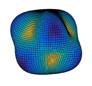
(a) $(\ell,m)=(4,3)$

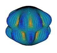
(b) $(\ell,m)=(8,7)$

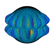
(c) $(\ell,m)=(16,15)$

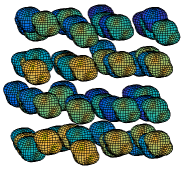
(d) Irregular Lattice

Figure 2: Example of test geometries. 2(a)–2(c) Example surfaces used in our experiments. The chart for surfaces is given by $\rho(\theta,\phi)=1+0.5Y_{\ell m}(\theta,\phi)$ where $Y_{\ell m}$ denotes the spherical harmonics. The color is the signed mean curvature. 2(d) A random lattice of $64$ shapes (arbitrarily colored).

In all experiments in this section, we precondition the local systems based on the framework discussed in Section 4.1. We construct a corresponding block-diagonal system $\mathsf{M}$ based spheres as $\Gamma_{i}$ and only considering the self interaction of each sphere. The QTT compressed form of this operator is denoted by $\mathtt{[}M]$. The QTT preconditioner is thus the product of two QTT matrices $\mathtt{[}M]$ and $\mathtt{[}Y]$. This provides a significant acceleration for the inversion algorithm by improving the conditioning of the local linear systems. It also provides an acceleration for the resulting inverse apply, as the resulting ranks of $\mathtt{[}M]$ and $\mathtt{[}Y]$ are observed to be smaller than those of their product.

For the sake of comparison with the volume integral experiments in Section 5.2, in Table 3 we report results for matrix compression and preconditioner setup in QTT form for $\varepsilon_{p}=10^{-3}$, for a regular lattice of surfaces with spherical topology and radius $\rho=1+0.5Y_{4,3}$. Unlike the cases in Tables 1 and 2, maximum ranks for both the forward matrix $\mathtt{[}A]$ and the matrix $\mathtt{[}Y]$ in the preconditioner show a relatively slow but steady increase with problem size $N$. As a consequence, both timings and inverse memory display sublinear growth with $N$. We note that in terms of rank behavior and the scaling of precomputation costs, the results presented in Table 3 are representative of all experiments presented in this section.

$N$	Time (sec)		Max Rank		Inverse Memory  (MB)
	Compress	Invert	Forward	Inverse
$\collectcell$3$840\endcollectcell$	$\centering 27.75\@add@centering$	$\centering 375.49\@add@centering$	$117$	$86~{}(49)$	$\centering 8.56\@add@centering$
$\collectcell$3$0720\endcollectcell$	$\centering 34.80\@add@centering$	$\centering 512.18\@add@centering$	$133$	$90~{}(49)$	$\centering 11.73\@add@centering$
$\collectcell$2$45760\endcollectcell$	$\centering 45.42\@add@centering$	$\centering 630.46\@add@centering$	$144$	$93~{}(50)$	$\centering 14.25\@add@centering$
$\collectcell$1$996080\endcollectcell$	$\centering 49.50\@add@centering$	$\centering 732.21\@add@centering$	$150$	$95~{}(50)$	$\centering 18.75\@add@centering$

Table 3: QTT preconditioner ranks and precomputation costs for the benchmark case. Compression and Inversion times, maximum QTT ranks, and memory requirements for the QTT decomposition algorithms for benchmark case on a regular cubic lattice. The QTT inverse is a product of two QTT matrices, a block-diagonal system for spherical surfaces $\mathtt{[}M]$ and the solution for the right-preconditioned system $\mathtt{[}X]$, as discussed in Section 4.1. We include maximum ranks for both QTT matrices, reporting those for block-diagonal $\mathtt{M}$ in parentheses, and reporting the aggregate memory requirements for both under “Inverse Memory”. The problem sizes range from $N=$3\,840$~{}(n=8,p=15)\text{ to }$1\,996\,080$~{}(n=4096,p=15)$, and the target accuracy for all algorithms to construct the QTT preconditioner is set to $\varepsilon_{p}=10^{-3}$. The model surface has radius $\rho=1+0.5Y_{4,3}$.

5.3.2 Comparison with other preconditioners

Multigrid, sparsifying preconditioners [68, 82], and hierarchical matrix preconditioners (using HSS-C, HIF, IFMM [19], or $\mathcal{H}$ inverse compression at low target accuracies) are a few options available for this type of problem.

We compare QTT’s setup costs (inversion time and memory requirements), its effectiveness in terms of iteration count for the iterative solver, and total solve time with those of multigrid and HIF. We use a two-level multigrid V-cycle, considered in [68], as preconditioner. Levels in this context are defined by the spherical harmonic order $p$. In our experiments, we choose $p_{\mathrm{coarse}}=\lceil p/2\rceil$ as the coarse level. We use the natural spectral truncation and padding for restriction and prolongation operators, and for smoothing, we use Picard iteration. The coarse-grid problems are solved iteratively using GMRES with tolerance $\varepsilon_{p}$. For HIF [42], we use a Matlab implementation kindly provided to us by Kenneth Ho and Lexing Ying.

For elliptic PDEs, multigrid provides an acceleration to the iterative solvers with almost negligible setup costs and storage requirements; however, its performance for integral equations is less understood. Fast direct solvers based on hierarchical matrix compression like HIF, on the other hand, have significantly large setup costs. Nevertheless, when preconditioners of the latter kind are affordable to construct for low accuracies, they present an effective preconditioner, reducing the number of iterations while incurring small cost associated with the application of the preconditioner, because of their quick apply.

Since QTT algorithms also provide a hierarchical decomposition of the inverse, we expect their performance to be similar to fast direct solvers such as HIF. We also anticipate that, due to its modest setup costs, it will enable the solution of problems with a large number of unknowns.

5.3.3 Overview of experiments

In order to successfully test the QTT preconditioner, we first establish a benchmark case, choosing a regular, cubic lattice of identical translates as our geometry. We expect this to be the most advantageous case for the QTT, as it is able to exploit any regularities present in the integration domain. We report our results in terms of matrix-vector applies required for the solve (Table 4). Since the multigrid approach proves to be limited in its effectiveness, we concentrate on a more detailed comparison of solve times against setup costs between QTT and HIF (Fig. 3).

We then devise two stress tests to determine the robustness of the QTT approach. First, we eliminate the regularity in the cubic lattice by randomly perturbing centers, radii and types of the surfaces that constitute it. As expected, a moderate increase in precomputation costs is observed for the QTT (Fig. 4). However, except for the lowest preconditioner accuracies, its performance in terms of iteration counts does not degrade when compared to the benchmark.

Finally, we subject both preconditioners to a series of experiments with progressively worse conditioning (we draw the surfaces in the lattice close to contact). However, for preconditioner accuracies $\varepsilon_{p}\leq 10^{-2}$, iteration counts and solve times for both preconditioners become practically independent of distance between surfaces, providing increasing speed-ups when compared to the unpreconditioned solve. We display results for $\varepsilon_{p}=10^{-3}$ (Figs. 5 and 6).

5.3.4 Benchmark

We test a cubic lattice of $q\times q\times q$ surfaces, for $n=q^{3}\in\{8,64,512,4096\}$, discretizing each surface using spherical harmonic basis of order $p\in\{15,24,35\}$, which requires $p+1$ collocation points in the latitude direction and $2p$ collocation points in the longitude direction. The total number of unknowns for each problem is then $N=2p(p+1)n$. We make all surfaces translations of a single shape on a regular lattice with spacing of $4$, which implies the closest distance between surfaces is slightly smaller than their diameter. To control surface complexity, we make their radius $\rho(\theta,\phi)=1+0.5Y_{\ell m}(\theta,\phi)$, where $Y_{\ell m}$ is the spherical harmonic function of order $(\ell,m)$.

For the matrix-vector apply, we use the FMMLIB3D library [26] for interactions between surfaces, and spectral quadrature for interactions within each surface [29]. We test three surfaces of increasing complexity by setting $\ell\in\{4,8,16\}$ and $m=\ell-1$, shown in Fig. 2.

The results of the tests on this lattice are reported in Table 4. For all problem sizes, we compare the number of matrix-vector applications for the unpreconditioned solve with those of the preconditioned solve with multigrid, QTT, and HIF. Each approximate-inverse preconditioner is constructed for a target accuracy of $\varepsilon_{p}=10^{-3}$ and is used within a GMRES solve with a tolerance of $\varepsilon=10^{-8}$ for relative residual and no restart.

$p$	$n$	$N$	Unpreconditioned			Multigrid			QTT			HIF
			$\ell=4$	$8$	$16$	$4$	$8$	$16$	$4$	$8$	$16$	$4$	$8$	$16$
$15$	$\collectcell$8$\endcollectcell$	$\collectcell$3$840\endcollectcell$	$129$	$401$	$1001$	$25~{}(140)$	$-$	$-$	$9$	$9$	$9$	$7$	$7$	$7$
$15$	$\collectcell$6$4\endcollectcell$	$\collectcell$3$0720\endcollectcell$	$153$	$255$	$991$	$25~{}(140)$	$-$	$-$	$11$	$11$	$9$	$7$	$7$	$9$
$15$	$\collectcell$5$12\endcollectcell$	$\collectcell$2$45760\endcollectcell$	$141$	$277$	$788$	$25~{}(140)$	$-$	$-$	$11$	$11$	$11$	$7$	$11$	$7$
$24$	$\collectcell$8$\endcollectcell$	$\collectcell$9$600\endcollectcell$	$153$	$229$	$617$	$21~{}(92)\phantom{0}$	$37~{}(180)$	$-$	$9$	$13$	$11$	$7$	$7$	$7$
$24$	$\collectcell$6$4\endcollectcell$	$\collectcell$7$6800\endcollectcell$	$141$	$207$	$677$	$21~{}(114)$	$37~{}(180)$	$-$	$11$	$13$	$15$	$9$	$7$	$7$
$24$	$\collectcell$5$12\endcollectcell$	$\collectcell$6$14400\endcollectcell$	$141$	$205$	$577$	$21~{}(103)$	$37~{}(180)$	$-$	$11$	$11$	$15$	$15$	$13$	$13$
$35$	$\collectcell$8$\endcollectcell$	$\collectcell$2$0160\endcollectcell$	$139$	$429$	$601$	$17~{}(16)\phantom{0}$	$25~{}(84)\phantom{0}$	$25~{}(140)$	$9$	$11$	$11$	$7$	$7$	$9$
$35$	$\collectcell$6$4\endcollectcell$	$\collectcell$1$61280\endcollectcell$	$143$	$187$	$651$	$17~{}(16)\phantom{0}$	$25~{}(73)\phantom{0}$	$25~{}(140)$	$9$	$11$	$11$	$9$	$7$	$9$
$35$	$\collectcell$5$12\endcollectcell$	$\collectcell$1$290240\endcollectcell$	$137$	$193$	$595$	$17~{}(16)\phantom{0}$	$25~{}(79)\phantom{0}$	$25~{}(140)$	$9$	$11$	$11$	$-$	$-$	$-$

Table 4: Matrix-vector apply count for the benchmark case. Comparison of unpreconditioned GMRES and preconditioned GMRES using multigrid, QTT, and HIF preconditioners for the exterior 3D Laplace problem over a regular lattice of $n$ model surfaces each with radius $\rho=1+0.5Y_{\ell m}$ where $\ell=\{4,8,16\}$ and $m=\ell-1$. Surfaces are represented in spherical harmonics basis and discretized with $2p(p+1)$ collocation points. The relative residual tolerance for GMRES is set to $\varepsilon=10^{-8}$ and GMRES is not restarted. For multigrid, the number of applies in the coarse GMRES solver (with $\varepsilon_{p}=10^{-2}$) is reported in parentheses. QTT and HIF approximate-inverse preconditioners are constructed with a target accuracy of $\varepsilon_{p}=10^{-3}$. Empty entries correspond to experiments in which either the preconditioned GMRES failed to converge in $100$ iterations or preconditioner setup costs were excessive.

From the results in Table 4, it can be readily observed that in this configuration the condition number of the problem, implied by number of iterations of the unpreconditioned solve, mostly depends on the individual surface complexity and not the number of surfaces $n$ or problem size $N$.

As we increase surface complexity (controlled by $\ell$), the average number of matrix-vector applies goes from $140$ to $240$ to $600$, rendering the unpreconditioned solve impractical. The multigrid preconditioner is easy and inexpensive to setup, but, as it is mentioned in [68], its performance suffers when the geometry is not resolved in the coarse grid, i.e. $p_{\mathrm{coarse}}$ is not large enough. In Table 4, we observe that after the individual surface geometry is resolved in the coarse grid, multigrid leads to a reduction in the iteration counts. However, this requires unnecessary over-resolution in the fine grid that is not required by the problem but by the preconditioner.

Furthermore, note that each multigrid cycle uses two matrix-vector applies at the fine level as well as a number of applies at the coarse level, and so the observed speedups with respect to the unpreconditioned solve are moderate. Additionally, for cases where both fine and coarse levels are resolved, such as $p=35$ and $\ell=4$, the number of coarse applies is still higher than the corresponding QTT and HIF direct solvers at the level equal to the multigrid coarse level ($p=15$ and $\ell=4$). Due to its mediocre performance, we choose not to further consider multigrid for our comparisons, focusing instead on comparing QTT and HIF direct-solver preconditioners.

As expected, both QTT and HIF display consistent performance across all cases considered and they display little or no dependence on surface complexity $\ell$, lattice size $n$, and number of unknowns $N$. For both approaches, the cost of an iteration is one matrix-vector apply and one fast apply of the corresponding compressed low-accuracy inverse. For most examples considered, applying the preconditioner takes only a fraction of the matrix-vector apply, allowing for considerable speedups.

In the following section, we explore different aspects of QTT and HIF preconditioners.

5.3.5 Comparison of direct-solver preconditioners

For a given model surface and problem size $N$, we report the setup costs (inversion time and storage) and the solve times using both direct solvers with inversion accuracies from $\varepsilon_{p}=10^{-1}\text{ to }10^{-3}$. In order to represent wall-clock time in a more meaningful way across experiments of different sizes, we normalize it in terms of the $\mathscr{O}\left(N\right)$ matrix-vector applies for the system matrix through FMM, hereinafter denoted by ${T}_{mv}(N)$. For $N>$500\,000$$, high inversion cost generally prevents us from constructing the HIF preconditioner.

In Fig. 3, we plot solve times against setup costs (inversion time and storage) for both QTT and HIF preconditioners. This allows us to identify distinct trade-offs in performance and efficiency, as well as to observe their scaling with respect to $N$ and $\varepsilon_{p}$.

Figure 3: Solve time vs. preconditioner setup time and memory for the benchmark case.  Semi-log plots for solve times, normalized by the matvec time ${T}_{mv}(N)$, vs. the required inversion time, also normalized by ${T}_{mv}(N)$, and storage requirements (in MB) for QTT and HIF preconditioners for $p=15$, $n=\{8,64,512,4096\}$ and $\varepsilon_{p}=10^{-1}\text{ to }10^{-3}$. Model surface has radius $\rho=1+0.5Y_{4,3}$. Because of $\log(N)$ complexity of QTT compression and inversion, QTT scheme becomes cheaper for larger problem sizes.

Solve time and speedup

As we increase the preconditioner accuracy $\varepsilon_{p}$, the number of iterations for the solve decreases while the cost of applying the corresponding preconditioner increases as QTT and HIF ranks increase. Both provide considerable speedups (unpreconditioned solve takes about $140{T}_{mv}(N)$), with HIF mostly yielding the highest when available. The main reason behind this is that the HIF apply has a more favorable dependence on $\varepsilon_{p}$ than the QTT apply. This is evident by the fact that the rise in preconditioner application cost causes the QTT solve time to plateau but it does not significantly affect the speedups yielded by HIF for the range of accuracies considered. For higher accuracies ($\varepsilon_{p}\lesssim 10^{-4}$), we observe a slight increase in solve times for QTT  as well as significant increases to setup costs for both solvers.

Inverse setup time

Figure 3(a) shows the solve time versus the setup time as $\varepsilon_{p}$ increases for different $N$. While HIF setup costs relative to ${T}_{mv}(N)$ increase as we increase the problem size, logarithmic scaling of the QTT inverse makes it more efficient (relative to ${T}_{mv}(N)$) as $N$ grows. This is one of the features that allows us to compute the QTT for large $N$, and it implies that for sufficiently large problem ($N=$245\,760$$ in this example), inverse setup can become cheaper than one matrix apply.

Inverse storage

Figure 3(b) depicts the required storage for each preconditioner as $\varepsilon_{p}$ increases. In this respect, QTT is extremely efficient and memory requirements have logarithmic scaling with respect to $N$ and do not exceed $100$ MB. On the other hand, the HIF inverse displays $\mathscr{O}\left(N\log N\right)$ scaling with large prefactor, requiring $10$s to $100$s of GB of memory to solve problems larger than a quarter million unknowns.

Dependence on surface complexity

As we increase the surface complexity by increasing the radial perturbation, we observe little to no difference in iteration counts (Table 4) as well as the solve times for both QTT and HIF. Thus, both alleviate the increase in condition number, evident by the increase in the corresponding number of unpreconditioned iterations. Though an increase in ranks and consequently in setup costs for the QTT inverse is observed, differences in rank distributions sharply decrease with $\varepsilon_{p}$, e.g., maximum ranks for $(\ell,m)=(8,7)$ case are roughly $3\times$ higher for $\varepsilon_{p}=10^{-1}$ and $1.5\times$ for $\varepsilon_{p}=10^{-3}$. The increase in costs for the HIF is predictably small due to the fact that it focuses on compressing far range interactions.

Effectiveness for different $\varepsilon$ and $\varepsilon_{p}$

To investigate the robustness of the preconditioners for higher target accuracies, in Table 5, we report how solve times vary across a range of target and preconditioner accuracies. Overall, the solve times (relative to ${T}_{mv}(N)$) for both solvers seem to be proportional to $\log(\varepsilon)$, and their performance with respect to $\varepsilon_{p}$ seems to replicate the case observed in Fig. 3 (which corresponds to $\varepsilon=10^{-8}$). This indicates that these direct solvers are extremely reliable as preconditioners.

$\varepsilon$	Unprec. Matvecs	QTT					HIF
		$\varepsilon_{p}=10^{-1}$	$10^{-1.5}$	$10^{-2}$	$10^{-2.5}$	$10^{-3}$	$10^{-1}$	$10^{-1.5}$	$10^{-2}$	$10^{-2.5}$	$10^{-3}$
$10^{-4\phantom{0}}$	$\phantom{0}81$	$13.2$	$9.2$	$8.4$	$6.1$	$7.4$	$7.3$	$6.5$	$5.7$	$5.7$	$5.7$
$10^{-6\phantom{0}}$	$107$	$19.4$	$14.8$	$13.3$	$11.1$	$10.6$	$13.5$	$10.9$	$8.0$	$5.7$	$5.7$
$10^{-8\phantom{0}}$	$141$	$25.5$	$20.9$	$18.2$	$13.7$	$13.8$	$17.7$	$15.3$	$10.3$	$8.0$	$8.0$
$10^{-10}$	$165$	$33.2$	$25.4$	$23.0$	$17.2$	$17.0$	$22.4$	$16.6$	$12.7$	$10.3$	$10.3$
$10^{-12}$	$187$	$39.0$	$30.5$	$27.9$	$20.9$	$20.2$	$28.9$	$22.8$	$17.0$	$12.6$	$10.3$

Table 5: Solve time for varying target and preconditioner accuracies.  Comparison of solve times relative to ${T}_{mv}(N)$ for QTT and HIF preconditioners for target accuracies $\varepsilon=10^{-4}\text{ to }10^{-12}$ and preconditioner accuracies $\varepsilon_{p}=10^{-1}\text{ to }10^{-3}$ for the model surface with radius $\rho=1+0.5Y_{4,3}$, and problem size $N=$245\,760$$ ($n=512,p=15$). Matvec counts for the unpreconditioned solve are also included for reference.

5.3.6 Perturbations of the benchmark

To further quantify the effectiveness of the QTT preconditioner, we perform experiments in which we perturb the uniform cubic lattice considered in the benchmark. Given the ineffectiveness of the multigrid preconditioner presented above, we only focus on the HIF preconditioner for comparison. Since one expects the QTT decomposition to exploit regularities and invariances in the geometry, this set of tests is aimed to measure its robustness when the regularity of the lattice is broken.

We construct each surface in the lattice with a radius of the form $\rho=1+rY_{\ell m}$, where $r$ is a random number in $(0,1)$, and $(\ell,m)$ is also randomly chosen between $(4,3)$ and $(8,7)$. Additionally, we perturb the location of the center of each surface in a random direction by up to $50$ percent of its diameter.

The results of this test are shown in Fig. 4. We observe similar behavior to the one seen in Fig. 3 for both solvers in terms of how solve times and setup costs behave as functions of the number of surfaces and preconditioner accuracy $\varepsilon_{p}$. Comparing the corresponding data for the QTT solver in these two figures, we observe a moderate increase in inverse setup times and storage for $n=256,$4\,096$\,(N\geq$245\,760$)$. This has an impact on the effective solve times in terms of matvecs, as the preconditioner apply is a bit more expensive. We also observe that for both QTT and HIF, $\varepsilon_{p}\simeq 10^{-1}$ seems to be much less effective than in the benchmark case. However, for $\varepsilon_{p}\leq 10^{-2}$, iteration counts and solve times display similar behavior to the benchmark case.

Figure 4: Solve vs. preconditioner setup and memory costs for irregular lattice and shapes. Semi-log plots for Solve times, normalized by matvec time ${T}_{mv}(N)$, for a given inversion time, also normalized by ${T}_{mv}(N)$, and storage requirements (in MB) for TT and HIF preconditioners. Each model surface has radius $\rho=1+rY_{\ell,\ell-1}$, where $\ell$ is randomly chosen to be 4 or 8 and $r$ is a random number in $(0,1)$. The location of the surfaces is also randomly perturbed.

Distance between Surfaces

As mentioned in Section 1, it is well known that conditioning of second kind integral equations tends to deteriorate as surfaces come close to contact. In order to test robustness in performance of the QTT and HIF preconditioners, we compare speedups and setup costs as we draw surface centers in the lattice close to each other in our experiments.

In Fig. 5, we report the speedups with respect to the average unpreconditioned solve, and plot them against the logarithm of the distance between surfaces in the lattice. Here, we use the number of unpreconditioned iterations as a surrogate for the problem conditioner number. As we draw the surfaces together, we observe that iteration counts and solve times for both preconditioners show a slight increase for low accuracy ($\varepsilon_{p}\simeq 10^{-1}$), becoming almost independent of distance for higher preconditioner accuracies ($\varepsilon_{p}\leq 10^{-2}$). This causes the effective speedup to increase as the unpreconditioned solve becomes more expensive, due to the increase in condition number.

Figure 5: Solve speedup vs. log distance between surfaces. Speedups, defined as the ratio between unpreconditioned and preconditioned solves and excluding the preconditioner setup time (see Fig. 6 for the setup costs), vs. log of the surface spacing in the lattice for QTT and HIF preconditioners with $\varepsilon_{p}=10^{-3}$.

Figure 6: Preconditioner setup and memory vs. log distance. Log of setup costs (in unpreconditioned solves) and storage requirements vs. log of the surface spacing in the lattice for QTT and HIF preconditioners with $\varepsilon_{p}=10^{-3}$.

In Fig. 6, we plot setup costs against the log of the distance between surfaces. Although displaying a sharp increase at first, preconditioner setup times increase at a pace much slower than the cost of the unpreconditioned solve, becoming more efficient. We again observe that as $N$ increases, the QTT preconditioner becomes more cost-effective, becoming just a fraction of an unpreconditioned solve for $N=$1\,966\,080$$. The rate at which storage requirements increase for both solvers also slows down as we reduce the distance, which means that they both display robust behavior in spite of the added complexity.

6 Conclusions

Motivated by the ongoing challenges to produce memory-efficient and reliable fast solvers for integral equations in complex geometries, we presented a robust framework employing the Tensor Train decomposition to accelerate the solution of volume and boundary integral equations in three dimensions.

In the context of volume integral equations on a regularly sampled domain, even for problems with up to 10 million unknowns and for relatively high target accuracies ($\varepsilon=10^{-6}$ to $10^{-10}$), we are able to produce a compressed inverse in no more than a few minutes and store it using tens of MBs of memory, When compared to the current state-of-the-art direct solvers in three dimensions, QTT is the only such fast direct solver to retain practical performance for large problem sizes.

In Section 5.3, we showed that the QTT framework is applicable to matrices arising from the discretization of boundary integral equations in complex, multiply-connected geometries. Nonetheless, for a given target accuracy, the QTT ranks are considerably higher than the volume integral case, rendering high target accuracies impractical. We thus proposed using a low target accuracy (e.g., $\varepsilon_{p}$ between $10^{-1}$ and $10^{-3}$) version of the QTT-based inverse as a preconditioner for the GMRES. We compared its effectiveness and cost against two alternative preconditioners, a simple multigrid and a low-accuracy HIF inverse.

By virtue of being a multilevel, low-accuracy direct solver, the QTT preconditioner matches the HIF in terms of reliability and robustness across all examples presented. We observe a clear trade-off between these two solvers: while HIF generally provides higher speedups, modest setup costs and storage requirements for the QTT make it extremely cost-effective. This is particularly the case for problems with a large number of unknowns, as setting up the QTT preconditioner typically becomes comparable to one solve for the range of target and preconditioner accuracies presented. In Section 5.3, this allowed us to solve an external Dirichlet problem for the Laplace equation in an irregular domain composed of $4096$ surfaces. The setup time for the QTT preconditioner for this example is as small as a few FMM applies and has a memory footprint of less than $10$ MB.

There are several extensions of this work that can be pursued. Here, all presented examples used a uniform hierarchical partition of the domain, corresponding to a uniform tree. We believe it is possible to extend the current implementation of the QTT algorithms to adaptive decompositions, using the connections between Tensor Train and other hierarchical decomposition techniques. Another research direction is generalizing of the QTT algorithms to obtain effective parallel scaling. It would be interesting to see whether the compute-bound nature of the QTT algorithms could be exploited to obtain good practical scaling.

7 Acknowledgments

We extend our thanks to Sergey Dolgov, Leslie Greengard, Ivan Oseledets, and Mark Tygert for stimulating conversations about various aspects of this work. We are also grateful to Matthew Morse, Michael O’Neil, and Shravan Veerapaneni for critical reading of this work and providing valuable feedback. We thank Kenneth Ho and Lexing Ying for kindly supplying the HIF code. Support for this work was provided by the US National Science Foundation (NSF) under grant DMS-1320621. E.C. acknowledges the support of the US National Science Foundation (NSF) through grant DMS-1418964.

Appendix A QTT decomposition as a hierarchical linear filter

In [65], the QTT decomposition is interpreted as a subspace approach, and in the case of the SVD based QTT decomposition (or more generally, when tensor cores are orthogonalized), as a fast method to compute a reduced orthogonal basis for structured tensors. We first show that the QTT decomposition can be viewed as a linear filter with respect to each of its cores. We recall from Section 2 that the compression algorithm proceeds by computing a sequence of low rank decompositions of unfolding matrices. For the $(k-1)\mathrm{th}$ unfolding matrix, we have the low rank decomposition

$$\mathsf{A}_{\mathcal{T}}^{k-1}(\overline{i_{1}\dots i_{k-1}},\overline{i_{k}\dots i_{d}})=\mathsf{U}_{k-1}(\overline{i_{1}\dots i_{k-1}},\alpha_{k-1})\mathsf{V}_{k-1}(\alpha_{k-1},\overline{i_{k}\dots i_{d}}).$$ (A.1)

We then vectorize $\mathpzc{A}_{\mathcal{T}}$, using the formula for products of matrices $\mathrm{vec}(\mathsf{ABC})=(\mathsf{C}^{T}\otimes\mathsf{A})\mathrm{vec}(\mathsf{B})$, to obtain

$$\mathrm{vec}(\mathpzc{A}_{\mathcal{T}})=(\mathsf{I}_{m_{k-1}}\otimes\mathsf{U}_{k-1})\mathrm{vec}(\mathsf{V}_{k-1}),$$ (A.2)

where $\mathsf{I}_{m_{k-1}}$ is the identity of size $m_{k-1}=\prod_{q\geq k}{n_{q}}$, and so the left factor is in fact a block-diagonal matrix of $m_{k-1}$ copies of $\mathsf{U}_{k-1}$. If $\mathsf{U}_{k-1}$ is orthogonal this factor is orthogonal as well, and we also have that $\mathsf{V}_{k-1}=\mathsf{U}_{k-1}^{\star}\mathsf{A}^{k-1}_{\mathcal{T}}$ and $\mathrm{vec}(\mathsf{V}_{k-1})=(\mathsf{I}_{m_{k-1}}\otimes\mathsf{U}_{k-1}^{\star})\mathrm{vec}(\mathpzc{A}_{\mathcal{T}})$. Applying this same identity, we obtain

$$\mathrm{vec}(\mathpzc{A}_{\mathcal{T}})=(\mathsf{V}^{T}_{k-1}\otimes\mathsf{I}_{p_{k-1}})\mathrm{vec}(\mathsf{U}_{k-1}),$$ (A.3)

where $p_{k-1}=\prod_{q<k}{n_{q}}$, and again if $\mathsf{V}^{T}_{k-1}$ is orthogonal, $\mathsf{U}_{k-1}=(\mathsf{V}^{T}_{k-1})^{\star}\mathsf{A}^{k-1}_{\mathcal{T}}$ and $\mathrm{vec}(\mathsf{U}_{k-1})=(\mathsf{V}^{T}_{k-1}\otimes\mathsf{I}_{p_{k-1}})^{\star}\mathrm{vec}(\mathpzc{A}_{\mathcal{T}})$.

Since the QTT compression algorithm can proceed via sweeps of low rank decompositions of unfoldings for $\mathsf{V}_{k}$ (left to right) or of $\mathsf{U}_{k}$ (right to left), we can iterate Eq. A.2 and Eq. A.3 separating one core at a time. Let $\mathpzc{G}_{k}$ denote the

$$k\mathrm{th}coreofthe{{QTT}}\ decompositionof\mathsf{A},and\mathsf{G}_{k}=\operatorname{reshape\,}(\mathpzc{G}_{k},[r_{k-1}n_{k},r_{k}]).Ifweapply\lx@cref{creftype~refnum}{eq:filter_left}k-1times,weobtain\begin{equation}\mathrm{vec}(\mathpzc{A}_{\mathcal{T}})=(\mathsf{I}_{m_{1}}\otimes\mathsf{G}_{1})(\mathsf{I}_{m_{2}}\otimes\mathsf{G}_{2})\dots(\mathsf{I}_{m_{k-1}}\otimes\mathsf{G}_{k-1})\mathrm{vec}(\mathsf{V}_{k-1}).\end{equation}Ifweapply\lx@cref{creftype~refnum}{eq:filter_right},wecanwriteanexplicitformulaforthek\mathrm{th}core\mathpzc{G}_{k}\begin{equation}\mathrm{vec}(\mathpzc{A}_{\mathcal{T}})=(\mathsf{I}_{m_{1}}\otimes\mathsf{G}_{1})\dots(\mathsf{I}_{m_{k-1}}\otimes\mathsf{G}_{k-1})(\mathsf{G}^{T}_{d}\otimes\mathsf{I}_{p_{d}r_{k-1}})\dots(\mathsf{G}^{T}_{k+1}\otimes\mathsf{I}_{p_{k+1}r_{k-1}})\mathrm{vec}(\mathpzc{G}_{k})\end{equation}\par Followingnotationfrom\cite[cite]{[\@@bibref{Number}{dolgov2013amen1}{}{}]},wedenotetheproductofthed-1matrixfactorsin\lx@cref{creftype~refnum}{eq:TT_reducedbasis}as\mathpzc{P}_{\neq k}(\mathsf{A}).Itscolumnsformareducedtensorbasisgeneratedby\{\mathsf{G}_{q}\}_{q\neq k},and\mathrm{vec}(\mathpzc{G}_{k})correspondstothecoefficientsthatreconstruct\mathsf{A}.Ifacorrectionstep(e.g.,using{{QR}})isimplementedtomake\{\mathsf{G}_{q}\}_{q<k}and\{\mathsf{G}^{T}_{q}\}_{q>k}orthogonal,then\mathpzc{P}_{\neq k}(\mathsf{A})isorthogonalaswell,andwehave\begin{equation}\mathrm{vec}(\mathpzc{G}_{k})=(\mathsf{G}^{T}_{k+1}\otimes\mathsf{I}_{p_{k+1}r_{k-1}})^{\star}\dots(\mathsf{I}_{m_{1}}\otimes\mathsf{G}_{1})^{\star}\mathrm{vec}(\mathpzc{A}_{\mathcal{T}})=\mathpzc{P}_{\neq k}(\mathsf{A})^{\star}\mathrm{vec}(\mathpzc{A}_{\mathcal{T}})\end{equation}\par Finally,wenotethatfrom\lx@cref{creftype~refnum}{eq:TT_applyfilter}anidentityfor\mathrm{vec}(\mathsf{A})canbereadilyfound,asthereexistsapermutationmatrix\Pi_{\mathcal{T}}suchthat\mathrm{vec}(\mathsf{A})=\Pi_{\mathcal{T}}\mathrm{vec}(\mathpzc{A}_{\mathcal{T}}).\par$$

Appendix B Setup of local linear systems for QTT inversion algorithms

The approximate inversion seeks to find $\mathsf{X}$ that satisfies $\mathsf{AX=I_{N}}$ or $\mathsf{AX+XA=2I_{N}}$ and to extract a QTT decomposition for $\mathsf{X}$. Given a set of proposed cores $\{\mathpzc{W}_{k}\}_{k=1}^{d}$ for $\mathsf{X}$ and fixing all but $\mathpzc{W}_{k}$, Eq. A.5 provides an explicit formula to interpret the QTT decomposition as an expansion in an orthonormal basis, with elements that depend on $\{\mathpzc{W}_{j}\}_{j\neq k}$ and coefficients $\mathrm{vec}(\mathpzc{W}_{k})$. That is, we can write $\mathrm{vec}(\mathsf{X})=\mathpzc{P}_{\neq k}(\mathsf{X})\mathrm{vec}(\mathpzc{W}_{k})$ where $\mathpzc{P}_{\neq k}(\mathsf{X})$ is orthogonal. Eq. 4.1 then becomes

$$(\mathsf{I}_{N}\otimes\mathsf{A})\mathpzc{P}_{\neq k}(\mathsf{X})\mathrm{vec}(\mathpzc{W}_{k})=\mathrm{vec}(\mathsf{I}_{N}).$$ (B.1)

From this one may readily notice that fixing all cores but $\mathpzc{W}_{k}$ yields an overdetermined linear system. Applying $\mathpzc{P}_{\neq k}(\mathsf{X})^{\star}$, we obtain the equivalent reduced system

$$\mathpzc{P}_{\neq k}(\mathsf{X})^{\star}(\mathsf{I}_{N}\otimes\mathsf{A})\mathpzc{P}_{\neq k}(\mathsf{X})\mathrm{vec}(\mathpzc{W}_{k})=\mathpzc{P}_{\neq k}(\mathsf{X})^{\star}\mathrm{vec}(\mathsf{I}_{N}).$$ (B.2)

The matrix in the linear system above is of size $n_{k}r_{k-1}r_{k}\times n_{k}r_{k}r_{k-1}$. Eq. B.2 allows us to solve for each core $\mathpzc{W}_{k}$ by projecting $\mathsf{X}$ onto this reduced basis in which $\mathpzc{W}_{k}$ is the only degree of freedom. We note that this necessarily leaves the size and rank of $\mathpzc{W}_{k}$ fixed, and as a consequence, some strategy must be implemented to increase ranks and accelerate convergence towards the solution.

• In DMRG methods, this issue is resolved by contracting two cores $\mathpzc{W}_{k},\mathpzc{W}_{k+1}$ at a time into a supercore

  $$\mathpzc{S}_{k}(\alpha_{k-1},\overline{i_{k}i_{k+1}},\alpha_{k+1})=\mathpzc{W}_{k}(\alpha_{k-1},i_{k},\alpha_{k})\mathpzc{W}_{k+1}(\alpha_{k},i_{k+1},\alpha_{k+1}),$$ (B.3)

  and solving the corresponding reduced system for $\mathpzc{S}_{k}$. The $k\mathrm{th}$ rank is now free (it was contracted in merging both cores) and it will be determined when newly computed $\mathpzc{S}_{k}$ is split into cores.

• In AMEN-type methods [20, 21], the residual $\mathsf{R}$ of this system is approximated in QTT form, and then it is used in an enrichment step to expand the reduced basis and allow for ranks to increase.

We also note that even though we present these reduced systems explicitly, in both DMRG and AMEN methods a recursive formula is employed to construct them as they cycle through the cores of $\mathsf{X}$. In fact, it is shown in [63] that if $\mathpzc{G}_{k}(\alpha_{k-1},\overline{i_{k}j_{k}},\alpha_{k})$ is the $k\mathrm{th}$ core of the QTT decomposition of $(\mathsf{I}_{N}\otimes\mathsf{A})$, then we can write the left-hand side of Eq. B.2 in the following form

$$\sum_{\alpha,\gamma,j}{\Psi_{k-1}(\alpha_{k-1},\beta_{k-1},\gamma_{k-1})\mathpzc{G}_{k}(\alpha_{k-1},\overline{i_{k}j_{k}},\alpha_{k})\Phi_{k}(\alpha_{k},\beta_{k},\gamma_{k})\mathpzc{W}_{k}(\gamma_{k-1},\overline{j_{k}p_{k}},\gamma_{k})},$$ (B.4)

where $\Psi_{k-1}$ is a function of $\{\mathpzc{G}_{j}\}_{j=1}^{k-1}$ and $\{\mathpzc{W}_{j}\}_{j=1}^{k-1}$, and $\Phi_{k}$ a function of $\{\mathpzc{G}_{j}\}_{j=k+1}^{d}$ and $\{\mathpzc{W}_{j}\}_{j=k+1}^{d}$. Moreover, recursive formulas $\psi$ and $\phi$ exist such that

$$\Psi_{k}=\psi(\Psi_{k-1},\mathpzc{G}_{k},\mathpzc{W}_{k})\quad\text{and}\quad\Phi_{k+1}=\phi(\Phi_{k-1},\mathpzc{G}_{k},\mathpzc{W}_{k}).$$ (B.5)

Finally, we note that Eq. B.4 may be interpreted as a compressed form of the matrix in the reduced linear system with a 3-dimensional QTT decomposition with cores $\Psi$, $\mathpzc{G}$, and $\Phi$. If this linear system is relatively small, the matrix in Eq. B.2 may be formed to solve this system densely. Otherwise, it is preferable to use the fast QTT matrix vector apply on the tensor decomposition in Eq. B.4 to solve this system using an iterative algorithm such as GMRES or BI-CGSTAB.

References

- [1] J.C. Aguilar and Y. Chen “High-order corrected trapezoidal quadrature rules for the Coulomb potential in three dimensions” In Computers & Mathematics with Applications 49.4 Elsevier, 2005, pp. 625–631
- [2] S. Ambikasaran and E. Darve “The Inverse Fast Multipole Method” In arXiv preprint arXiv:1407.1572, 2014, pp. 1–25
- [3] W. Austin, G. Ballard and T.G. Kolda “Parallel Tensor Compression for Large-Scale Scientific Data” In arXiv preprint arXiv:1510.06689, 2015
- [4] J. Barnes and P. Hut “A hierarchical force-calculation algorithm” In Nature 324, 1986, pp. 4
- [5] M. Bebendorf “Hierarchical LU decomposition-based preconditioners for BEM” In Computing (Vienna/New York) 74.3, 2005, pp. 225–247
- [6] M. Bebendorf “Hierarchical matrices” A means to efficiently solve elliptic boundary value problems 63, Lecture Notes in Computational Science and Engineering Berlin: Springer-Verlag, 2008, pp. xvi+290
- [7] I. Benedetti, M. H. Aliabadi and G. Davì “A fast 3D dual boundary element method based on hierarchical matrices” In International Journal of Solids and Structures 45.7-8, 2008, pp. 2355–2376
- [8] M. Benzi “Preconditioning Techniques for Large Linear Systems: A Survey” In Journal of Computational Physics 182.2, 2002, pp. 418–477
- [9] S. Börm “Efficient numerical methods for non-local operators” -matrix compression, algorithms and analysis 14, EMS Tracts in Mathematics European Mathematical Society (EMS), Zürich, 2010, pp. x+432
- [10] S. Börm, L. Grasedyck and W. Hackbusch “Hierarchical matrices” In Lecture notes 21, 2003
- [11] J.P. Boyd “Chebyshev and Fourier Spectral Methods” Dover Publications Inc., 1999
- [12] B. Carpentieri, I. S. Duff and L. Giraud “A Class of Spectral Two-Level Preconditioners” In SIAM Journal on Scientific Computing 25.2, 2003, pp. 749–765
- [13] B. Carpentieri, I. S. Duff, L. Giraud and G. Sylvand “Combining Fast Multipole Techniques and an Approximate Inverse Preconditioner for Large Electromagnetism Calculations” In SIAM Journal on Scientific Computing 27.3, 2005, pp. 774–792
- [14] T.F. Chan, W. P. Tang and W. L. Wan “Wavelet sparse approximate inverse preconditioners” In BIT Numerical Mathematics 37.3, 1997, pp. 644–660
- [15] S. Chandrasekaran, P. Dewilde, M. Gu, W. Lyons and T. Pals “A fast solver for HSS representations via sparse matrices” In SIAM Journal on Matrix Analysis and Applications 29.1 SIAM, 2006, pp. 67–81
- [16] S. Chandrasekaran, M. Gu and T. Pals “A fast ULV decomposition solver for hierarchically semiseparable representations” In SIAM Journal on Matrix Analysis and Applications 28.3 SIAM, 2006, pp. 603–622
- [17] H. Cheng, Z. Gimbutas, P-G. Martinsson and V. Rokhlin “On the compression of low rank matrices” In SIAM Journal on Scientific Computing 26.4 SIAM, 2005, pp. 1389–1404
- [18] E. Corona, P.G. Martinsson and D. Zorin “An () direct solver for integral equations on the plane” In Applied and Computational Harmonic Analysis Elsevier, 2014
- [19] P. Coulier, H. Pouransari and E. Darve “The inverse fast multipole method: using a fast approximate direct solver as a preconditioner for dense linear systems” In arXiv preprint arXiv:1508.01835, 2015
- [20] S. Dolgov and D.V. Savostyanov “Alternating minimal energy methods for linear systems in higher dimensions” In Part I: SPD systems, arXiv preprint 1301, 2013
- [21] S. Dolgov and D.V. Savostyanov “Alternating minimal energy methods for linear systems in higher dimensions. Part II: Faster algorithm and application to nonsymmetric systems” In arXiv preprint arXiv:1304.1222, 2013
- [22] S. Dolgov, B. Khoromskij and D. Savostyanov “Superfast Fourier transform using QTT approximation” In Journal of Fourier Analysis and Applications 18.5 Springer, 2012, pp. 915–953
- [23] R. Duan and V. Rokhlin “High-order quadratures for the solution of scattering problems in two dimensions” In Journal of Computational Physics 228.6 Elsevier, 2009, pp. 2152–2174
- [24] A. Gillman “Fast direct solvers for elliptic partial differential equations”, 2011
- [25] A. Gillman, P.M. Young and P.G. Martinsson “A direct solver with complexity for integral equations on one-dimensional domains” In Frontiers of Mathematics in China Springer, 2012, pp. 1–31
- [26] Z Gimbutas and L Greengard “FMMLIB3D 1.2, FORTRAN libraries for fast multiple method in three dimensions”, http://www.cims.nyu.edu/cmcl/fmm3dlib/fmm3dlib, 2011 URL: http://www.cims.nyu.edu/cmcl/fmm3dlib/fmm3dlib
- [27] L. Giraud, S. Gratton and E. Martin “Incremental spectral preconditioners for sequences of linear systems” In Applied Numerical Mathematics 57.11-12, 2007, pp. 1164–1180
- [28] G.H. Golub and C.F. Van Loan “Matrix computations” JHU Press, 2012
- [29] IG Graham and IH Sloan “Fully discrete spectral boundary integral methods for Helmholtz problems on smooth closed surfaces in ” In Numerische Mathematik 92.2 Springer, 2002, pp. 289–323
- [30] A. Grama, V. Kumar and A. Sameh “Parallel Hierarchical Solvers and Preconditioners for Boundary Element Methods” In Proceedings of the 1996 ACM/IEEE Conference on Supercomputing 20.1, 1996, pp. 337–358
- [31] L. Grasedyck “Hierarchical low rank approximation of tensors and multivariate functions” In Lecture notes of the Zürich summer school on Sparse Tensor Discretizations of High-Dimensional Problems, 2010
- [32] L. Grasedyck, D. Kressner and C. Tobler “A literature survey of low-rank tensor approximation techniques” In GAMM-Mitteilungen 36.1 Wiley Online Library, 2013, pp. 53–78
- [33] L. Greengard and J-Y. Lee “A direct adaptive Poisson solver of arbitrary order accuracy” In Journal of Computational Physics 125.2 Elsevier, 1996, pp. 415–424
- [34] L. Greengard and V. Rokhlin “A fast algorithm for particle simulations” In Journal of Computational Physics 73.2 Elsevier, 1987, pp. 325–348
- [35] L. Greengard and V. Rokhlin “A new version of the fast multipole method for the Laplace equation in three dimensions” In Acta numerica, 1997 6, Acta Numer. Cambridge: Cambridge Univ. Press, 1997, pp. 229–269
- [36] L. Gürel and T. Malas “Iterative Near-Field Preconditioner for the Multilevel Fast Multipole Algorithm”, 2010
- [37] W. Hackbusch “Tensorisation of vectors and their efficient convolution” In Numerische Mathematik 119.3 Springer, 2011, pp. 465–488
- [38] W. Hackbusch and B.N. Khoromskij “Blended kernel approximation in the H-matrix techniques” In Numerical linear algebra with applications 9.4 Wiley Online Library, 2002, pp. 281–304
- [39] W. Hackbusch and Z.P. Nowak “On the fast matrix multiplication in the boundary element method by panel clustering” In Numerische Mathematik 54.4 Springer, 1989, pp. 463–491
- [40] W. Hackbusch, B. Khoromskij and E. Tyrtyshnikov “Hierarchical Kronecker tensor-product approximations” In Journal of Numerical Mathematics jnma 13.2, 2005, pp. 119–156
- [41] W. Hackbusch, B. Khoromskij and E. Tyrtyshnikov “Approximate iterations for structured matrices” In Numerische Mathematik 109.3 Springer, 2008, pp. 365–383
- [42] K. Ho and L. Ying “Hierarchical interpolative factorization for elliptic operators: integral equations” In Communications on Pure and Applied Mathematics Wiley Online Library, 2015
- [43] K.L. Ho and L. Greengard “A fast direct solver for structured linear systems by recursive skeletonization” In SIAM Journal on Scientific Computing 34.5 SIAM, 2012, pp. 2507–2532
- [44] S. Kapur and V. Rokhlin “High-order corrected trapezoidal quadrature rules for singular functions” In SIAM Journal on Numerical Analysis 34.4 SIAM, 1997, pp. 1331–1356
- [45] V.A. Kazeev and B. Khoromskij “Low-rank explicit QTT representation of the Laplace operator and its inverse” In SIAM Journal on Matrix Analysis and Applications 33.3 SIAM, 2012, pp. 742–758
- [46] V. Khoromskaia and B.N. Khoromskij “Grid-based lattice summation of electrostatic potentials by assembled rank-structured tensor approximation” In Computer Physics Communications 185.12 Elsevier, 2014, pp. 3162–3174
- [47] B. Khoromskij “-quantics approximation of - tensors in high-dimensional numerical modeling” In Constructive Approximation 34.2 Springer, 2011, pp. 257–280
- [48] B. Khoromskij, S. Sauter and A. Veit “Fast quadrature techniques for retarded potentials based on TT/QTT tensor approximation” In Computational Methods in Applied Mathematics Comput. Methods Appl. Math. 11.3, 2001, pp. 342–362
- [49] B.N. Khoromskij “Tensor numerical methods for multidimensional PDES: theoretical analysis and initial applications” In ESAIM: Proceedings and Surveys 48 EDP Sciences, 2015, pp. 1–28
- [50] B.N. Khoromskij “-quantics approximation of - tensors in high-dimensional numerical modeling” In Preprint 55/2009, Max-Planck Institute for Math. in the Sciences, Leipzig, 2009 URL: http://www.mis.mpg.de/publications/preprints/2009/prepr2009-55.html
- [51] T.G. Kolda and B.W. Bader “Tensor decompositions and applications” In SIAM review 51.3 SIAM, 2009, pp. 455–500
- [52] R. Kress, V. Maz’ya and V. Kozlov “Linear integral equations” Springer, 1989
- [53] O. Marin, O. Runborg and A. Tornberg “Corrected trapezoidal rules for a class of singular functions” In IMA Journal of Numerical Analysis 34.4 Oxford University Press, 2014, pp. 1509–1540
- [54] P-G. Martinsson, V. Rokhlin and M. Tygert “On interpolation and integration in finite-dimensional spaces of bounded functions” In Communications in Applied Mathematics and Computational Science 1.1 Mathematical Sciences Publishers, 2007, pp. 133–142
- [55] P.G. Martinsson and V. Rokhlin “A fast direct solver for boundary integral equations in two dimensions” In Journal of Computational Physics 205.1 Elsevier, 2005, pp. 1–23
- [56] K. Nabors, T. Korsmeyer and J. White “Multipole-Accelerated Preconditioned Iterative Methods For Solving Three-Dimensional Mixed First And Second Kind Integral Equations” In SIAM Journal on Scientific and Statistical Computing 15.3, 1994, pp. 713–735
- [57] Noël M. Nachtigal, Satish C. Reddy and Lloyd N. Trefethen “How Fast are Nonsymmetric Matrix Iterations?” In SIAM Journal on Matrix Analysis and Applications 13.3, 1992, pp. 778–795
- [58] V. Olshevsky, I.V. Oseledets and E. Tyrtyshnikov “Tensor properties of multilevel Toeplitz and related matrices” In Linear algebra and its applications 412.1 Elsevier, 2006, pp. 1–21
- [59] V. Olshevsky, I.V. Oseledets and E. Tyrtyshnikov “Superfast inversion of two-level Toeplitz matrices using Newton iteration and tensor-displacement structure” In Recent Advances in Matrix and Operator Theory Springer, 2008, pp. 229–240
- [60] I.V. Oseledets “Tensors inside of matrices give logarithmic complexity” In Preprint 4, 2009
- [61] I.V. Oseledets “Approximation of Matrices Using Tensor Decomposition” In SIAM Journal on Matrix Analysis and Applications 31.4 SIAM, 2010, pp. 2130–2145
- [62] I.V. Oseledets “TT-Toolbox 2.2”, 2012 URL: https://github.com/oseledets/TT-Toolbox
- [63] I.V. Oseledets and S.V. Dolgov “Solution of linear systems and matrix inversion in the TT-format” In SIAM Journal on Scientific Computing 34.5 SIAM, 2012, pp. A2718–A2739
- [64] I.V. Oseledets and E. Tyrtyshnikov “TT-cross approximation for multidimensional arrays” In Linear Algebra and its Applications 432.1 Elsevier, 2010, pp. 70–88
- [65] I.V. Oseledets and E. Tyrtyshnikov “Algebraic wavelet transform via quantics tensor train decomposition” In SIAM Journal on Scientific Computing 33.3 SIAM, 2011, pp. 1315–1328
- [66] I.V. Oseledets, E. Tyrtyshnikov and N. Zamarashkin “Tensor-train ranks for matrices and their inverses” In Comput. Methods Appl. Math. 11.3, 2011, pp. 394–403
- [67] D. Pissoort, E. Michielssen, D.V. Ginste and F. Olyslager “A rank-revealing preconditioner for the fast integral-equation-based characterization of electromagnetic crystal devices” In Microwave and Optical Technology Letters 48.4, 2006, pp. 783–789
- [68] B. Quaife and G. Biros “On preconditioners for the Laplace double-layer in 2D” In arXiv preprint arXiv:1308.1937, 2013, pp. 1–26
- [69] A. Rahimian, S.K. Veerapaneni, D. Zorin and G. Biros “Boundary integral method for the flow of vesicles with viscosity contrast in three dimensions”, 2015, pp. 766–786
- [70] V. Rokhlin “Rapid solution of integral equations of classical potential theory” In J. Comput. Phys. 60.2, 1985, pp. 187–207
- [71] Y. Saad and M.H. Schultz “GMRES: A generalized minimal residual algorithm for solving nonsymmetric linear systems” In SIAM Journal on Scientific and Statistical Computing 7.3 SIAM, 1986, pp. 856–869
- [72] P. Starr and V. Rokhlin “On the numerical solution of two-point boundary value problems. II” In Comm. Pure Appl. Math. 47.8, 1994, pp. 1117–1159
- [73] J. Tausch and J. White “Preconditioning first and second kind integral formulations of the capacitance problem” In Methods 4, 1996, pp. 96
- [74] J. Tausch and J. White “Preconditioning and fast summation techniques for first-kind boundary integral equations” In IMACS International Symposium on Iterative Methods in Scientific Computation, 1997
- [75] E. Tyrtyshnikov “Incomplete cross approximation in the mosaic-skeleton method” In Computing 64.4 Springer, 2000, pp. 367–380
- [76] E. Tyrtyshnikov “Tensor ranks for the inversion of tensor-product binomials” In Journal of computational and applied mathematics 234.11 Elsevier, 2010, pp. 3170–3174
- [77] S.A. Vavasis “Preconditioning for Boundary Integral Equations” In SIAM Journal on Matrix Analysis and Applications 13.3, 1992, pp. 905–925
- [78] H.A. Vorst “Bi-CGSTAB: A fast and smoothly converging variant of Bi-CG for the solution of nonsymmetric linear systems” In SIAM Journal on Scientific and Statistical Computing 13.2 SIAM, 1992, pp. 631–644
- [79] Y. Wang, J. Lee and J. Zhang “A short survey on preconditioning techniques for large-scale dense complex linear systems in electromagnetics” In International Journal of Computer Mathematics 84.8, 2007, pp. 1211–1223
- [80] A. J. Wathen “Preconditioning” In Acta Numerica 24.April, 2015, pp. 329–376
- [81] J. Xia, S. Chandrasekaran, M. Gu and X.S. Li “Fast algorithms for hierarchically semiseparable matrices” In Numerical Linear Algebra with Applications 17.6 Wiley Online Library, 2010, pp. 953–976
- [82] L. Ying “Sparsifying preconditioner for the lippmann-schwinger equation” In Multiscale Modeling & Simulation 13.2, 2014, pp. 1–18