Seeing relativity – I. Ray tracing in a Schwarzschild metric to explore the maximal analytic extension of the metric and making a proper rendering of the stars

Abstract

We present an implementation of a ray tracing code in the Schwarzschild metric. We aim at building a numerical code with a correct implementation of both special (aberration, amplification, Doppler) and general (deflection of light, lensing, gravitational redshift) relativistic effects so as to simulate what an observer with arbitrary velocity would see near, or possibly within, the black hole. We also pay some specific attention to perform a satisfactory rendering of stars. Using this code, we then show several unexplored features of the maximal analytical extension of the metric. In particular, we study the aspect of the second asymptotic region of the metric as seen by an observer crossing the horizon. We also address several aspects related to the white hole region (i.e., past singularity) seen both from outside the black hole, inside the future horizon and inside the past horizon, which gives rise to the most counter-intuitive effects.

I Introduction

The visual aspect of black holes is a frequent public outreach question but for decades, did not generate much interest among physicists or astronomers. A somewhat caricatural example of this is given by S. Chandrasekhar famous book on black holes chandrasekhar83 , where the visual aspect of a Schwarzschild black hole is summarized in a tiny picture on page 130, the caption of which being rather pedantic and obscure for a non expert reader since the author does not describe the picture as a sketch of the angular size of a Schwarzschild black hole as a function of the distance of a static observer, but rather talks about the “cone of avoidance” of null geodesics (which technically means the same thing).

Still, the problem of black hole visualization had already drawn some sparse attention at the time of Chandrasekhar book in the more difficult context of the Kerr metric, the earliest work being that of Bardeen in 1972 bardeen72 and later Luminet luminet79 . An increasing number of work were published afterward, a very incomplete subset of which lies in Refs. fukue88 ; viergutz93 ; marck95 ; fanton97 ; falcke00 ; hamilton04 ; beckwith05 . In the recent years, a much larger amount of work has been performed on black hole visualization. The main reason for this growing interest came from obvious astronomical constraints: the largest black hole (in term of angular size) seen from Earth, Sgr A*, has an angular diameter of order of 60 $\mu$as gillessen09 , which is unobservable by conventional astronomical devices, but which should be at reach within less than a decade with the advent of long baseline interferometry in the millimetric domain, thus making the actual aspect of a black hole silhouette become a problem of astronomical relevance. Consequently, most of those recent works are motivated by actual astrophysical observational projects of our Galactic center such as GRAVITY gravity or the Event Horizon Telescope eht , see, e.g., vincent11 ; broderick11 ; chan13 ; broderick14 , but some others were focused on what could be seen if an observer stood close to a black hole muller10 ; thorne15 thus being less relevant from an observational perspective, but more focused on the diversity of physical effects that can arise in the vicinity of a black hole. Our work fits within this second category.

The case of special relativity is much simpler and has deserved an earlier attention as early as 70 years ago with the pioneering sketches of Gamow gamow . (Although it is often said that special relativity was also a source of artistic inspiration for S. Dali in his famous painting “La persistència de la Memoria” (The Persistence of Memory, 1931), it actually does not seem to be the case dali .) The increasingly easier access to large computing facilities has progressively allowed the completion of excellent works by, for example Ruder and Nollert ruder-nollert or Searle et al. searle .

The aim of this paper is to present here a numerical code that implements most of the relativistic effects that arise when simulating what an observer would see in a black hole metric, focusing here on the Schwarzschild one. The Schwarzschild metric is the simplest black hole metric that exists. It is both astrophysically relevant (contrarily to the Reissner-Nordstrom one) and simple to study thanks to its spherical symmetry (contrarily to the Kerr on Kerr-Newmann metrics). In particular, as we shall see, it is possible to perform a rather nice and efficient rendering of pointlike light sources (i.e., stars) thanks to spherical symmetry, an issue which was not addressed satisfactorily till now. Although initially made for teaching purpose, these simulations allowed an exhaustive study of the metric and was very easy to adapt to the whole Schwarzschild metric, i.e. its maximal analytic extension, or Kruskal-Szekeres coordinates, where we found a series of unexpected visual effect which where rather counter-intuitive even for an experienced relativity scientist.

The paper is structured as follows. The camera (i.e., the way to project a part of the celestial sphere on a two-dimensional screen) is described in Sec. II. We then address the way to simulate the way a background sky is distorted both by special relativistic effects and the presence of a gravitational field (Sec. III). This first, naive, method can be significantly improved in term of computational time by explicitly using the fact that the metric is spherically symmetric as explained in Sec. IV. The results of this section are then used to make a very rapid and satisfactory rendering of the stars (or any pointlike light source), as explained in Sec. V. In Sec. VI, we list all the data that we use in order to produce examples of realistic images. We computed many pictures using this method which are useful in getting a better representation of special and general relativistic effects. Since many of these correspond more a new way to show old results rather than actual new results, we have put then in Appendix B. Still keeping in mind that this work can have some obvious popular science application, we explain in Sec.VII how to rather easily adapt them for planetarium projection using the standards of this field. This being done, we present in Sec. VIII some results we obtained when exploring the parameter space of the simulated images, and that were not, or not significantly emphasized in existing literature. For example, we compute the angular size of the horizon both at horizon crossing and close to the singularity. Then, we explore in Sec. IX some new features which happen when considering the maximal analytic extension of the metric, both inside and outside the horizon.

In what follows, we shall use the $(+---)$ convention for the metric signature. We place ourselves in a coordinates systems such that $c=G=1$, and keep the second as time unit, so that a distance of $1$ corresponds to one light second (i.e. approximately $3\times 10^{5}\;{\rm km}$) and a mass of $1$ corresponds to around $2\times 10^{5}$ Solar masses. As long as our in interested in making single images, the mass of the black hole does not matter, however, since only the ratio $r/M$, $r$ being the radial coordinate, matters. Unless otherwise specified we shall place ourselves in a spherical version of the so-called Schwarzschild coordinates, where the line element is written

$${\rm d}s^{2}=\left(1-\frac{2M}{r}\right){\rm d}t^{2}-\frac{{\rm d}r^{2}}{1-\frac{2M}{r}}-r^{2}\left({\rm d}\theta^{2}+\sin^{2}\theta{\rm d}\varphi^{2}\right).$$ (1)

II Defining the observer and its camera

We assume that the images we want to simulate are those that would be seen by an observer is endowed with a four-velocity $u_{\rm obs}^{\mu}$ that either results from a chosen trajectory (possibly following a geodesic or not) or from any user defined data. We do not take into account the fact that the observer is unlikely to survive to his/her journey within the black hole environment either because of arbitrarily large acceleration imposed by some non geodesic motion (staying static just above the horizon, for example) or because of arbitrarily large tidal effects endured close or within a black hole of sufficiently small mass. We simulate here standard images and do not address much the interesting issue of stereoscopic vision as was done in Ref. hamilton10 .

The camera orientation is described by a set of three unit orthogonal spacelike vectors, $X^{\mu}$, $Y^{\mu}$, $Z^{\mu}$ all of which are orthogonal to $u_{\rm obs}^{\mu}$. We define the orientation of the camera by the following assumptions:

• Any pixel of the screen can be seen as pointing toward a spacelike direction $N^{\mu}$ belonging to the $X^{\mu}$, $Y^{\mu}$, $Z^{\mu}$ hyperplane, where $N_{\mu}N^{\mu}=-1$, i.e., a photon hitting the screen coming from this direction possesses a wave vector proportional to $u_{\rm obs}^{\mu}-N^{\mu}$, which is evidently a null vector;

• The $Z^{\mu}$ direction points toward the center of the screen, i.e. photons hitting the center of the screen possesses a wavevector proportional to $u_{\rm obs}^{\mu}-Z^{\mu}$;

• The $X^{\mu}$ direction is associated to the central horizontal line of the screen in the sense that any photon hitting this part of the screen possesses a wavevector proportional to $u_{\rm obs}-aZ^{\mu}-cX^{\mu}$, where $a^{2}+c^{2}=1$, the value of $a$ and $c$ being determined by the pixel position and the choice of projection (see below);

• The $Y^{\mu}$ direction is associated to the central vertical line of the screen in the sense that any photon hitting this part of the screen possesses a wavevector proportional to $u_{\rm obs}-a^{\prime}Z^{\mu}-bY^{\mu}$, where $a^{\prime 2}+b^{2}=1$ (same remark as for $a$ and $c$ above).

Moreover, we do not focus here on simulating images seen from a large distance, in which one can perform a flat sky approximation. Instead, the viewing angle of the picture is supposed to be of same order of normal viewing condition, an opening angle of $90^{\circ}$ being a relevant choice for this purpose. The exact association between a pixel of coordinates $(i,j)$ and the corresponding direction $N^{\mu}(i,j)$ is somewhat arbitrary and depends on the choice of projection one wants to use. A natural choice is spherical projection, which reproduces the exact view on the screen provided that the person viewing the screen is set at the proper position with respect to it, that depends on the view opening angle. When not at the proper position, any shape on the screen becomes distorted. For example, the circular silhouette of a Schwarzschild black hole no longer appears circular. In order to evade this problem, a natural choice corresponds to stereographic projection for which the circular shape of the black hole silhouette is always a circle on the screen. We shall make this choice for flat projections. If one denotes $\alpha$ the half of the opening angle of the picture along the horizontal direction, and $R$ and $C$ the number of rows and columns of the screen then the pixel coordinates $(i,j)$ of a given direction $N^{\mu}$ is given by

$$i = \frac{C+1}{2}+\frac{C}{2\tan(\alpha/2)}\frac{-X_{\mu}N^{\mu}}{1+(-N_{\mu}Z^{\mu})},$$ (2)

$$j = \frac{R+1}{2}+\frac{C}{2\tan(\alpha/2)}\frac{-Y_{\mu}N^{\mu}}{1+(-N_{\mu}Z^{\mu})}.$$ (3)

(The minus sign at the denominator of each formula comes from the signature convention we adopt here.) We assume here that the pixel coordinates ranges from $1$ to $C$ in along the horizontal direction, number $1$ being on the left, and from $1$ to $R$ in the vertical direction, from top to bottom, following the usual computer convention. In the usual case where both $R$ and $C$ are even, the center of the screen (i.e., $N^{\mu}=Z^{\mu}$) does not correspond to a pixel but to the common corner of the four adjacent central pixels of coordinates $(C/2,R/2)$, $(C/2+1,R/2)$, $(C/2,R/2+1)$ and $(C/2+1,R/2+1)$. We also assume that pixels are square, i.e, that pixel aspect ratio is exactly 1. In the case where one produces pictures with non square pixels such as for standard video formats (e.g., 576i 4:3, which has a pixel ratio of 12:11), then one has to rescale the second formula (3) along the vertical direction according to the imposed pixel ratio.

The inverse transform that allows to compute the direction $N^{\mu}$ as a function of pixel coordinates can be written in two steps by defining the intermediate spacelike vector $W^{\mu}$,

$$W^{\mu} = Z^{\mu}+\frac{2\tan(\alpha/2)}{C}\times$$

$$\left[\left(i-\frac{C+1}{2}\right)X^{\mu}+\left(j-\frac{R+1}{2}\right)Y^{\mu}\right],$$

$$N^{\mu} = -Z^{\mu}+2\frac{W^{\mu}}{-W_{\mu}W^{\mu}}.$$ (5)

Now, the way one defines the vectors $X^{\mu}$, $Y^{\mu}$, $Z^{\mu}$ is done as follows:

• We start from what we call a reference tetrad that is defined for each event of the space-time. This tetrad is orthonormal and is made of one timelike vector $T^{\mu}$ and three spacelike vectors $R^{\mu}$, $\Theta^{\mu}$, $\Phi^{\mu}$, the label of which are of course related to the coordinate system (1) (see later).

• All these vectors are Lorentz transformed according to the unique Lorentz boost $\Lambda^{\mu}_{\;\nu}$ that transforms the tetrad timelike vector $T^{\mu}$ into the observer’s velocity $u_{\rm obs}^{\mu}$ and leaves invariant any vector orthogonal to both of them.

• The three spacelike vector obtained after performing the Lorentz boost on $\Theta^{\mu}$, $\Phi^{\mu}$, $R^{\mu}$, i.e., $A^{\mu}\equiv\Lambda^{\mu}_{\;\nu}\Theta^{\nu}$, $B^{\mu}\equiv\Lambda^{\mu}_{\;\nu}\Phi^{\nu}$, $C^{\mu}\equiv\Lambda^{\mu}_{\;\nu}R^{\nu}$ are then rotated by a space rotation $R^{\mu}_{\;\nu}$ that leaves $u_{\rm obs}^{\mu}$ invariant in order to give the three camera vectors $X^{\mu}=R^{\mu}_{\;\nu}A^{\nu}$, $Y^{\mu}=R^{\mu}_{\;\nu}B^{\nu}$, $Z^{\mu}=R^{\mu}_{\;\nu}C^{\nu}$.

Simple algebra allows to prove that the $\Lambda^{\mu}_{\;\nu}$ components are (see, e.g., gourgoulhon10 ):

$$\Lambda^{\mu}_{\;\nu}=\delta^{\mu}_{\nu}-\frac{1}{1+\gamma}(T^{\mu}+u_{\rm obs}^{\mu})(T_{\nu}+u_{{\rm obs}\;\nu})+2u_{\rm obs}^{\mu}T_{\nu},$$ (6)

where we have defined $\gamma$ as the Lorentz factor

$$\gamma\equiv T_{\mu}u_{\rm obs}^{\mu},$$ (7)

so that one indeed has $\Lambda^{\mu}_{\;\nu}T^{\nu}=u_{\rm obs}^{\mu}$ and $\Lambda^{\mu}_{\;\nu}(-u_{\rm obs}^{\nu}+2\gamma T^{\nu})=T^{\mu}$, as expected.

Before computing the components of this matrix one of course has to define those of the reference tetrad vectors. A natural choice can be to use a normalized version of the standard spherical Schwarzschild coordinates (i.e., $T^{\mu}\propto\partial/\partial t$, $R^{\mu}\propto\partial/\partial r$ and so on), however such a choice is only valid outside the black hole, since the then defined $T^{\mu}$ would no longer be timelike within the black hole. It is therefore more appropriate to define the tetrad that can be associated to a freely falling observer starting from infinity with zero velocity and zero angular momentum. This is a rather common choice of Zero Angular Momentum Observers (ZAMO), see, e.g., thorne86 . Such set of observers’ four-velocity will correspond to the vector $T^{\mu}$. Then we define $R^{\mu}$ as the unique unit spacelike vector spanned by $\partial/\partial t$ and $\partial/\partial r$ that is orthogonal to $T^{\mu}$ and that reduces to $\partial/\partial r$ at infinity. We keep $\Theta^{\mu}$ and $\Phi^{\mu}$ unchanged as compared to the first ansatz above. Anticipating on the analysis of the maximal analytic extension of the metric, we use a subscript ${\rm I}$ to the vectors $T^{\mu}$ and $R^{\mu}$ as we will need to perform another choice for those vectors in some situations. Those vector components are:

$$T^{\mu}_{\rm I}=\left(\begin{array}[]{c}\frac{1}{1-\frac{2M}{r}}\\ -\sqrt{\frac{2M}{r}}\\ 0\\ 0\end{array}\right)\; \quad R^{\mu}_{\rm I}=\left(\begin{array}[]{c}-\frac{\sqrt{\frac{2M}{r}}}{1-\frac{2M}{r}}\\ 1\\ 0\\ 0\end{array}\right),$$ , (16)

$$\Theta^{\mu}=\left(\begin{array}[]{c}0\\ 0\\ \frac{1}{r}\\ 0\end{array}\right)\; \quad\Phi^{\mu}=\left(\begin{array}[]{c}0\\ 0\\ 0\\ \frac{1}{r\sin\theta}\end{array}\right).$$ , (25)

This tetrad is defined everywhere in the astrophysically relevant part of the Schwarzschild metric, regardless one is inside or outside the black hole (except, of course, at $r=0$).

Regarding the rotation $R^{\mu}_{\nu}$, we do not compute its components explicitly. Rather, we define its three associated Euler angle. We first rotate $A^{\mu}$ and $B^{\mu}$ by an angle $\phi$ around $C^{\mu}$. Then, we rotate the newly obtained $A^{\prime\mu}$ and $C^{\mu}$ by and angle $\vartheta$ around the newly obtained $B^{\prime\mu}$, and finally, we perform a new rotation by an angle $\psi$ around the new $C^{\prime\mu}$. In other words, we process along the following sequence:

$$\left(\begin{array}[]{c}A^{\prime\mu}\\ B^{\prime\mu}\end{array}\right) = \left(\begin{array}[]{cc}\cos\phi&\sin\phi\\ -\sin\phi&\cos\phi\end{array}\right)\left(\begin{array}[]{c}A^{\mu}\\ B^{\mu}\end{array}\right),$$ (32)

$$\left(\begin{array}[]{c}Z^{\mu}\\ A^{\prime\prime\mu}\end{array}\right) = \left(\begin{array}[]{cc}\cos\vartheta&\sin\vartheta\\ -\sin\vartheta&\cos\vartheta\end{array}\right)\left(\begin{array}[]{c}C^{\mu}\\ A^{\prime\mu}\end{array}\right),$$ (39)

$$\left(\begin{array}[]{c}X^{\mu}\\ Y^{\mu}\end{array}\right) = \left(\begin{array}[]{cc}\cos\psi&\sin\psi\\ -\sin\psi&\cos\psi\end{array}\right)\left(\begin{array}[]{c}A^{\prime\prime\mu}\\ B^{\prime\mu}\end{array}\right).$$ (46)

III Drawing the celestial sphere – Naive version

As stated above, any photon seen originating from unit spacelike direction $N^{\mu}$ orthogonal to the observer velocity $u_{\rm obs}^{\mu}$ is endowed with a wave vector proportional to $k^{\mu}\propto u_{\rm obs}-N^{\mu}$. Once such vector is defined (up to some unimportant proportionality constant), knowing from which direction on the celestial sphere it originates amounts to propagate it backward in time (i.e. backward in its affine parameter $p$) the geodesic equation

$$\frac{{\rm d}k^{\mu}}{{\rm d}p}+\Gamma^{\mu}_{\nu\rho}k^{\nu}k^{\rho}=0,$$ (47)

where the $\Gamma^{\mu}_{\nu\rho}$ are the usual Christoffel symbols.

III.1 First case – Observer outside the horizon

If one works in the usual Schwarzschild spherical coordinates, then this set of equations is written as (see, e.g.,carroll97 ):

$$\frac{{\rm d}k^{t}}{{\rm d}p} = -\frac{A^{\prime}}{A}k^{t}k^{r},$$ (48)

$$\frac{{\rm d}k^{r}}{{\rm d}p} = -\frac{1}{2}AA^{\prime}(k^{t})^{2}+\frac{1}{2}\frac{A^{\prime}}{A}(k^{r})^{2}$$

$$+Ar\left((k^{\theta})^{2}+\sin^{2}\theta(k^{\varphi})^{2}\right),$$

$$\frac{{\rm d}k^{\theta}}{{\rm d}p} = -\frac{2}{r}k^{r}k^{\varphi}+\sin\theta\cos\theta(k^{\varphi})^{2},$$ (50)

$$\frac{{\rm d}k^{\varphi}}{{\rm d}p} = -\frac{2}{r}k^{r}k^{\varphi}-2\frac{\cos\theta}{\sin\theta}k^{\theta}k^{\varphi},$$ (51)

where we have set

$$A\equiv 1-\frac{2M}{r},$$ (52)

and where the prime denotes a derivative with respect to the $r$ coordinate (i.e., $A^{\prime}=2M/r^{2}$). These equation have of course to be solved together with the position equation:

$$\frac{{\rm d}x^{\mu}}{{\rm d}p}=k^{\mu}.$$ (53)

In practice, this set of equations is solved using an adaptative 4^thorder Runge-Kutta method inspired from the Numerical Recipes numrec . One step that has to be implemented with some care is the choice of the time step. As we will see later, two numerically tricky zones lie at $r=2M$ (horizon crossing) and $r=3M$ (light circle crossing, where radial motion can be slow and unstable whereas orthoradial motion must be carefully computed; see Appendix A). Therefore, the timestep choice is essentially given by the following choices:

• If the geodesic is recessing away from the black hole (when propagated backward in time) with $r$ already larger than $4M$, the timestep is chosen proportional to $r^{2}$, so that infinity (or, in practice, a very large value of $r/M$) is reached after a few steps (typically 4 or 5);

• If the geodesic approaches the black hole, then one chooses a timestep proportional to $r-4M$;

• If one lies within the $r=4M$ sphere, then a sufficiently small timestep is chosen so as to insure both stability of the integration and monitoring a possible horizon crossing (see later).

If one is outside the black hole and if we do not consider the maximal analytic extension of the metric, then this equation has to be solved only when the geodesics originates from infinity. By setting the constants of motion $E$ and $L^{2}$ by their standard definition, i.e.,

$$E \equiv \pi_{t}=g_{t\mu}k^{\mu}=Ak^{t},$$ (54)

$$L^{2} \equiv r^{4}\left((k^{\theta})^{2}+\sin^{2}\theta(k^{\varphi})^{2}\right),$$ (55)

then the geodesic equation needs to be computed if and only if

1. $L^{2}/E^{2}\geq 27M^{2}$ and $r>3M$, or

2. $L^{2}/E^{2}\leq 27M^{2}$ and $k^{r}<0$.

(Since this is a fairly well-known result we just recall it here, but for the sake of completeness derive it in Appendix A.)

If none of these conditions are satisfied, this means that the geodesic originates from the past event horizon, or, from an astrophysically realistic point of view, from the infinitely redshifted surface of the collapsing object which gave birth to the black hole as it was passing through the horizon. If one does not works within the maximal analytic extension of the metric, then such geodesics do not carry any photon and the corresponding pixel is black. If, on the contrary, one works in the maximal analytic extension and want to compute from which part of the singularity a given null geodesic originates from, then the geodesic can be propagated back to the past singularity and imaged provided one decides of some emission properties of the past singularity (see IX).

For geodesics originating from infinity, one obtains at the end of integration a wavevector $k_{\infty}^{\mu}$ whose only non negligible components are $k_{\infty}^{t}$ and $k_{\infty}^{r}$, the two others tending to 0 when $r$ tends to infinity because of angular momentum conservation. Regarding the position, $r$ and $t$ both tend to minus infinity with their difference $r-t$ being almost constant, and $\theta$ and $\varphi$ tend to be constant. This is because as long as the radial coordinate $r$ is much larger than the impact parameter $b\equiv L/E$, the geodesic can be considered as (almost) purely radial and originating from the direction defined by the above mentioned $\theta$ and $\varphi$.

In addition, one can compute the redshift $z$ of the photons we receive. This is done through the standard formula

$$1+z=\frac{k^{t}_{\infty}}{k^{\mu}u_{{\rm obs}\;\mu}}=\frac{E}{k^{\mu}u_{{\rm obs}\;\mu}},$$ (56)

where the numerator is evaluated (as the subscript indicates) at infinity, whereas the denominator is computed at observer’s position before integration. Note that this formula include both the kinetic and gravitational redshift.

Once the initial direction of the photon and the redshift are known, we can draw the corresponding pixel.

III.2 Second case – Observer inside the horizon and/or within the maximal analytic extension

The set (48–51) is valid only when geodesics do not cross the horizon. Therefore, if the observer is within the horizon, it is not possible to simulate what he/she sees of the celestial sphere using these equations. In order to do so, one has to use another system of coordinates, the most natural of which being that of Kruskal kruskal60 . In this case, the subset of coordinates $(t,r)$ have to be replaced by the subset $(U,V)$ defined by the following procedure. First, we define the so-called “tortoise” coordinate $r^{*}$ by

$$r^{*}=r+2M\ln\left|\frac{r}{2M}-1\right|,$$ (57)

so that

$${\rm d}r^{*}=\frac{{\rm d}r}{1-\frac{2M}{r}}.$$ (58)

Here, $r^{*}$ is a growing function of $r$ outside the horizon and a decreasing function of $r$ inside (regardless one considers the maximal analytic extension or not). Then, we define the null outgoing and ingoing coordinates $u$ and $v$ such as

$$u \equiv t+r^{*},$$ (59)

$$v \equiv t-r^{*},$$ (60)

and finally $U$ and $V$ are defined through

$$U \equiv \epsilon\exp\left(+\frac{u}{4M}\right),$$ (61)

$$V \equiv \eta\exp\left(-\frac{v}{4M}\right).$$ (62)

The constant $\epsilon,\eta=\pm 1$ are then chosen so that both $U$ and $V$ are future-oriented. Anticipating on what we will do in §VIII, IX, we will need to know the values of $\epsilon$ and $\eta$ in all the regions of the maximal analytic extension of the metric. Since this is rarely done in the literature (see, e.g.,  carroll97 ; hawking73 ; wald84 ), their value are summarized in Table 1, using the following labels for the regions: we call I our asymptotic region, II the black hole interior beyond the future event horizon, III the other asymptotic region and and IV the region beyond the past event horizon. (In Ref. hawking73 , our regions III and IV are called I’ and II’, respectively, and IV and III in Ref. wald84 ).

Region	Remark	$\epsilon$	$\eta$
I	$t$ is future-oriented	$1$	$-1$
II	$r$ is past-oriented	$1$	$1$
III	$t$ is past-oriented	$-1$	$1$
IV	$r$ is future-oriented	$-1$	$-1$

Table 1: Values of the parameters $\epsilon$ and $\eta$ as defined in Eqns (61–62). Their value allow the null coordinates $U$ and $V$ to with proper time regardless the observer position within the maximal extension of the Schwarzschild metric. Which of the variable $t$ or $r$ of the standard Schwarzschild coordinates that is bound to grow or decrease with proper time from any timelike geodesics is also given.

This choice for $\epsilon$ and $\eta$ also possesses the nice property to ensure that the product $UV$ can be expressed as a function of $r$ only, without any reference to $\epsilon$ or $\eta$ :

$$UV=-\exp\left(\frac{r}{2M}\right)\frac{r-2M}{2M}.$$ (63)

This being set, the set of geodesic equations (48–51) has then to be replaced by the following set of equations

$$\ddot{U} = -\frac{\partial_{U}F}{F}\dot{U}^{2}-\frac{r}{F}\partial_{U}r\;\left(\dot{\theta}^{2}+\sin^{2}\theta\dot{\varphi}^{2}\right),$$ (64)

$$\ddot{V} = -\frac{\partial_{V}F}{F}\dot{V}^{2}-\frac{r}{F}\partial_{V}r\;\left(\dot{\theta}^{2}+\sin^{2}\theta\dot{\varphi}^{2}\right),$$ (65)

$$\ddot{\theta} = \cos\theta\sin\theta\dot{\varphi}^{2}-\frac{2\dot{\theta}}{r}(\dot{U}\partial_{U}r+\dot{V}\partial_{V}r),$$ (66)

$$\ddot{\varphi} = -2\frac{\cos\theta}{\sin\theta}\dot{\theta}\dot{\varphi}-\frac{2\dot{\varphi}}{r}(\dot{U}\partial_{U}r+\dot{V}\partial_{V}r),$$ (67)

where we have set

$$F\equiv g_{UV}=-\frac{8M^{2}A}{UV},$$ (69)

$A$ being defined in Eq. (52) and where we have used the following intermediate quantities

$$\partial_{U}r = \frac{2MA}{U},$$ (70)

$$\partial_{V}r = \frac{2MA}{V},$$ (71)

$$\partial_{U}F = \frac{2MAF^{\prime}}{U},$$ (72)

$$\partial_{U}F = \frac{2MAF^{\prime}}{V},$$ (73)

in which $F^{\prime}$ denotes the derivative of $F$ with respect to $r$, which is quite straightforwardly deduced from Eq. (63) and can be written as

$$F^{\prime}=\left(-\frac{1}{2M}+A^{\prime}(r)\right)\frac{F}{A}.$$ (74)

Since $F^{\prime}$ only appears when multiplied by $A$ the set of equation is regular at horizon crossing.

The set of variables $U,V$ is well suited for horizon crossing and is in principle defined everywhere on the maximal analytic extension of the manifold. In practice it is however not possible to use it everywhere since the exponential dependence of both $U$ and $V$ in term of $r$ and $t$ make it numerically impossible to use as soon as one goes several Schwarzschild radii away from the black hole. Therefore, we adopt the following procedure in order to choose the coordinate system:

• From the knowledge of constants $E$ and $L^{2}$ and position, we determine whether the geodesic we are interested in has any chance to cross horizon;

• If not, then we use the Schwarzschild coordinates $r,t$;

• If so, then we check whether one is close to the horizon;

• If not, then we keep the Schwarzschild coordinates;

• If so, then we switch to Kruskal coordinates;

• Then we keep on using Kruskal coordinates till horizon has been crossed, in which case we switch back to Schwarzschild coordinates.

• In the specific case on is interested in an observer in region II crossing null geodesics coming from region IV, we always keep the Kruskal coordinates.

The only arbitrariness here lies in where exactly we decide to switch from one coordinate system to the other. In practice, the radial motion of photon is determined by and effective potential $V(r)$ given in Eq. (121). This potential show that in some case, a geodesic may spend a large amount of time around $r=3M$ (the so-called light circle or photon sphere) around which the one dimensional radial motion is unstable. Therefore, we choose to impose that the light circle crossing is made using Schwarzschild coordinates $r,t$.

III.3 From geodesic equation solution to RGB values

Whichever method we used to solve the geodesic equation, we can compute, for any pixel of our screen, from which the corresponding null geodesic originates from. If it originates from the past horizon, the corresponding pixel is black (unless the special case of Sec. IX), or it corresponds to a direction of the celestial sphere. Assuming that we have a map of this celestial sphere, i.e. from a full sky survey of the sky (see §VI), we can determine which pixel of the celestial sphere the direction we found corresponds to. However, this is not the end of the story.

In a perfectly realistic situation, we should have at our disposal a spectral map of the celestial sphere, i.e., spectroscopic data for each direction of it. Then we would modify the spectrum according to the computed redshift and then compute the eye response to that observed spectrum and then deduce the corresponding RGB coordinates of the pixel. But in practice, we are limited by the fact that we do not have such spectral information. This therefore gives the correct colors of the sky seen by the observer only when redshift is negligible, and there is no simple way to compute the color or intensity change of the celestial sphere due to the redshift, therefore we shall compensate this by various visual artifacts. For example, it is possible to define by hand the spectral information for each direction of the celestial sphere that matches the pixel color (black body plus emission lines, for example). However, we found that if we deal properly with the stars (see §V), the rendering of the rest of the celestial sphere was not of crucial importance as the overall rendering was, by far, dominated by the stars. Therefore, we chose to let the pixel hue unchanged and simply shift the intensity of the corresponding pixel of the celestial sphere by a factor that is a monotonous function of $(1+z)^{-1}$. We found that a satisfactory function was a power law of $(1+z)^{-1}$ for negative $z$ (i.e., blueshift) and an exponential of $-(1+z)$ for positive $z$ (i.e., redshift).

IV Drawing the celestial sphere – Sophisticated version

In the Section above, the number of geodesic equations we have to solve is equal to the number of pixels of the screen and can therefore easily reach several millions and severely affect the computational time for each picture. The situation is worsened by the fact that some smoothing may be necessary when computing the image, i.e., one may need to split one pixel into several subpixels, compute the color of all of them and average the result accordingly, see Ref. thorne15 .

Such a large number of integrations of the geodesic equation is actually not necessary because, as is well known, is a spherically symmetric metric, null geodesics are described by a single parameter, which can be taken to be the impact parameter $b=L/E$. Moreover, we are considering a situation where the only information about the geodesics we are interested in is the amount of deflection the photon trajectory experiences between the direction it travels at the observer’s position and the direction it was traveling at infinity. Therefore, we adopt the following procedure:

• Before computing the image, we solve the geodesics equation for a freely falling observer (or the one that defines our reference tetrad, with four-velocity $T^{\mu}$) for all possible angles $\delta$ between the geodesic and the radial direction $R^{\mu}$. This amounts to sample, in some appropriate way, all the values of the geodesic impact parameter.

• For each of these geodesics we obtain the angle $\delta-\chi$ by which the geodesics has been deflected before reaching the observer.

• We sample this quantity sufficiently by computing a moderately large number of geodesics so that the both functions $\chi(\delta)$ and its inverse $\delta(\chi)$ are well sampled.

• Then, for each pixel of the image, compute the angle $\delta$ between the corresponding null geodesic and the radial direction, and identify the plane into which the photon trajectory lies.

• We rotate within this plane the observer position by an angle $\chi+\pi$ so as to identify the point of the celestial sphere the photon originates from.

• We compute the RGB coordinates of the pixel one has to draw following the selected assumptions for redshift rendering, see §III.3.

The angle $\delta$ we use here is defined with respect to our reference tetrad (16–25). This means that it is given by the formula

$$\cos\delta=\frac{-k^{\mu}R_{\mu}}{k^{\nu}T_{\nu}},$$ (75)

or, equivalently, this means that we will integrate a bunch of geodesics whose wavevector $k^{\mu}$ is defined as

$$k^{\mu}\propto T^{\mu}+\cos\delta R^{\mu}+\sin\delta(\cos\varpi\Phi^{\mu}+\sin\varpi\Theta^{\mu}).$$ (76)

We can of course choose, without loss of generality, $\varpi=0$ and have only yo sample $\delta$. With this definition, a radial geodesic originating from the black hole past horizon is described by an angle $\delta=0$, and a radial geodesic originating from past null infinity is described by $\delta=\pi$. Because of spherical symmetry, when we compute the $\chi(\delta)$ function, we can place ourselves in the equatorial plane at the same $r$ coordinate as the observer and by considering equatorial geodesics only that start from the $x$ axis (i.e., our freely falling fiducial observer lies at coordinates $(t,r,\pi/2,0)$ and $\varpi=0$ in Eq. (76)). From this position and this wavevector, we propagate the geodesic backward in time till it reaches very large values of $r$ (typically larger than $10^{10}M$, but the exact value does not matter). We then obtain the azimuthal angle $\varphi_{\infty}$ with respect to the observer of the corresponding origin of the geodesic (for example, $\varphi_{\infty}=0$ for $\delta=\pi$, and the angle $\chi$ is then given by

$$\chi=\varphi_{\infty}+\pi-\delta.$$ (77)

Should there be no aberration nor deflection of light, then one would just have $\chi=0$, i.e., $\varphi_{\infty}=\delta-\pi$, regardless of the observer’s position and velocity. An example of deviation function $\chi(\delta)$ (or, in fact, $\varphi_{\infty}(\delta)$) is given in Figure 1.

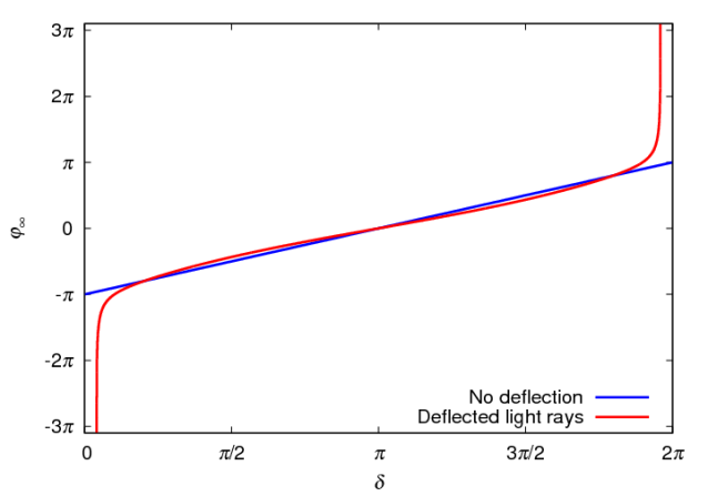
Figure 1: An example of the deviation function $\varphi_{\infty}(\delta)$. The one shown here was computed for a freely falling observer on a Schwarzschild black hole at coordinate distance $r=30M$. In the absence of any relativistic effect, the function $\varphi_{\infty}(\delta)$ would trivially reduce to $\varphi_{\infty}=\delta-\pi$, shown in dashed lines. But the adjunction of aberration (since the observer is freely falling) and light deflection modify it, only slightly away from the black hole ($\delta$ close to $\pi$), or much more importantly toward the black hole ($\delta$ close to $0$ or $2\pi$). The black hole angular radius is given by the first value of $\delta$ for which $\varphi_{\infty}$ diverges. Here, the function was sampled so as to include values of $|\varphi_{\infty}|$ slightly larger than $5\pi$, which is sufficient to include any visible ghost images of stars in most situations.

The main characteristic of this function is that it diverges for the extreme values of $\delta$ for which the function is defined, a fact that is recalled in Appendix A and that is usually called the zoom-and-whirl effect giampedakis02 .

Note that the two angles $\delta$ and $\chi$ are associated to somewhat different contexts: $\delta$ is an angle defined by a freely falling observer in the Schwarzschild metric, whereas $\chi$ corresponds to an angle measured by a static observer in Minkowski space whose origin and orientation matches that of the Schwarzschild metric.

In practice, sampling this $\chi(\delta)$ function necessitates a few thousands of geodesics to be computed, i.e. a factor between $10^{2}$ and $10^{3}$ less than the brute force computation of the previous section assuming million pixel sized images. This situation is also enhanced by the fact that it suffices to perform the computation in the equatorial plane, so that, in practice, there is no need to consider the $\theta$ and $k^{\theta}$ variable in the ODE system (48–51,53).

Then, once this deflection function is computed, all what we need to do rely on very simple trigonometric operations for all each pixel of the screen and some search in the deflection function $\chi(\delta)$ pre-computed array. More importantly, the deviation function will further be used in the next section (through its inverse) in order to perform a very clean rendering of the stars.

V Drawing the stars

The main drawback of the sky rendering above is that it is not well suited to include point sources. A point source such as a star will never appear as perfectly pointlike. Because of diffraction, a point source will always appears as possessing a small but non zero angular size typically of circular shape (with possibly diffraction patterns) and can, in principle, belong to the pixellized version of the celestial sphere. However, when distorting the image of such a source, its appearance will also be distorted. As is well known, amplification due to gravitational lensing goes with a large amount of shear, so that an initially circular pattern will become quite elongated. This is not the way this source should appear because given the actual smallness of a star angular size, even in a strong lensing regime it should be considered a pointlike and its visual finite angular size would only result in the optical distortions caused by the observation apparatus. Consequently, it is not possible to consider stars as “points” that would be “impainted” on the celestial sphere, and stars (or any almost pointlike sources) should be processed using a different procedure.

V.1 Direct ray tracing from interpolation

Since we work in a Schwarzschild metric, any direction on the celestial sphere will possess an infinity of images seen from any observer point of view, even though most of these images will be extremely faint and close to the edge of the black hole silhouette (see, e.g., chandrasekhar83 ). Since the metric is spherically symmetric, any geodesic is planar and all the geodesics starting from the same point of the celestial sphere and reaching the observer belong to the same plane.

If we have some star catalog, what we know about a given star is its position $\bm{n}^{*}$ on the celestial sphere. We also know the observer position within the metric, and consequently we know the plane spanned by the observer, the black hole and the star, as well as the angle between the observer radial position and and star position, $\varphi^{*}_{\infty}$. We can choose the orientation of the star-observer-black hole plane so that $\varphi_{\infty}^{*}$ lies between $0$ (observer is between the star and the black hole) and $\pi$ (black hole is between the observer and the star). We can now invert the procedure outlined in the previous section, with the extra complication that for a given $\delta_{0}$ such that $\varphi_{\infty}(\delta_{0})=\varphi_{\infty}^{*}$, there exists other values of $\delta$ that we shall note $\delta_{k}$ such that

$$\varphi_{\infty}(\delta_{k})=\varphi_{\infty}^{*}+2k\pi.$$ (78)

Those are the ghost images of the star. There exists an infinity of such images as long as the function $\varphi_{\infty}(\delta)$ diverges (see Fig. 1), which is the case for the Schwarzschild metric. These ghost images are not difficult to find numerically as long as the function $\varphi_{\infty}(\delta)$ is accurately sampled. We therefore can find without difficulty the apparent position of any ghost image of any star.

V.2 Amplification

This being done, we know the direction under which we see a given image of the star. However, because of both aberration and lensing, the actual (microscopic) angular area of the star will be different, and hence its luminosity. In order to take account for this, we shall define two directions very close to that where the star (or, in fact, one of its image) is seen. Since we work here in the observer’s frames, the directions we are talking about can be expanded in term of the spacelike vectors $X^{\mu}$, $Y^{\mu}$, $Z^{\mu}$ and can be considered as Euclidean three-vectors which we shall write in bold notations and the direction into which the (image of the) star is seen will be written $\bm{n}$. In order to define two directions infinitesimally close to $\bm{n}$, we choose one direction $\bm{n}^{\prime}$ that is different from $\bm{n}$. This can be for example either $\bm{x}$ or $\bm{z}$ (one may choose the one among these two which has the smallest dot product with $\bm{n}$). Then, we compute

$$\bm{n}^{\perp}_{1}=\frac{\bm{n}\wedge\bm{n}^{\prime}}{|\bm{n}\wedge\bm{n}^{\prime}|},$$ (79)

and then

$$\bm{n}^{\perp}_{2}=\bm{n}\wedge\bm{n}_{1}^{\perp}.$$ (80)

We then choose two small quantities $\delta_{1}$ and $\delta_{2}$ and define

$$\bm{n}_{1} = \bm{n}+\bm{\delta n}_{1}^{\perp}=\bm{n}+\delta_{1}\bm{n}_{1}^{\perp},$$ (81)

$$\bm{n}_{2} = \bm{n}+\bm{\delta n}_{2}^{\perp}=\bm{n}+\delta_{2}\bm{n}_{2}^{\perp}.$$ (82)

Up to $O(\delta_{1,2}^{2})$ terms, these two vectors are units vectors that are very close to $\bm{n}$. Now, it is obvious that the solid angle $\Omega$ spanned by three directions $\bm{n}$, $\bm{n}_{1}=\bm{n}+\bm{\delta n}_{1}^{\perp}$ and $\bm{n}_{2}=\bm{n}+\bm{\delta n}_{2}^{\perp}$ is given by the formula

$$\Omega=\bm{n}\cdot(\bm{\delta n}_{1}^{\perp}\wedge\bm{\delta n}_{2}^{\perp})=\bm{n}\cdot(\bm{n}_{1}\wedge\bm{n}_{2}).$$ (83)

Equivalently, if we propagate the null geodesics which originate from these three direction till the celestial sphere, we obtain three direction on the celestial sphere, $\bm{n}^{*}$, $\bm{n}^{*}_{1}$ and $\bm{n}_{2}^{*}$ which span a solid angle $\Omega^{*}$ given by

$$\Omega^{*}=\bm{n}^{*}\cdot(\bm{n}_{1}^{*}\wedge\bm{n}_{2}^{*}).$$ (84)

With these notations, the amplification or de-amplification factor $f$ induced both by lensing and aberration is simply written as

$$f=\frac{\Omega}{\Omega^{*}}.$$ (85)

(This is, of course, nothing more than solving in this particular context the relevant part of the optical scalar equation, i.e., convergence, see, e.g., Ref. seitz94 .) Computing this factor numerically is in fact not necessary. There exists an analytical formula for amplification due to aberration, and the deflection function $\chi(\delta)$ (or, in fact, the derivative of its inverse) allows after some algebra to address the lensing part. However in practice this does not allow to perform significant enhancement in term of CPU time so that we won’t address this here but rather keep it for future work.

V.3 Effective drawing of the star

In the two last subsections, we explained how to determine the position of (the image of) a star on the observer’s screen, in addition to its redshift and the amplification of its light because of aberration and lensing. For simplicity, we shall assume here that stars have a black-body type emission whose temperature is given by their spectral type (O and A being hotter, K and M cooler).

If one wants to compute the colour perceived by human eye a given light source (in term of, say, its RGB coordinate of a computer screen), one has to know the eye perception for each visible monochromatic frequency. These data are called the spectral tristimulus values are have been tabulated since a long time by the dedicated authority, the International Commission on Illumination (CIE) cie . For simplicity, we assume that eye response do not depend on light intensity, that is, we somewhat questionably assume that the observer’s vision always works in diurnal (photopic) mode rather than in low brightness (scotopic) environment. This allows more colorful hues for stars than what we are used to. In any case, if one starts from a light source with a given spectrum, one can compute the RGB values of this source by using the trichromatic tables delivered by the CIE.

In practice, with the assumptions we make about the star spectra, the procedure is the following:

1. Prior to launching the code, we have processed our star catalog in order to transform each star’s spectral type and magnitude in the V-band into a bolometric magnitude $m_{*}$ and a surface temperature $T_{*}$.

2. For each image of each star, we compute the corresponding redshift $z$ and amplification factor $f$.

3. We deduce that the star image possesses an apparent (in the sense of observer-dependent) bolometric magnitude and temperature given by

   $$m_{*}^{\rm obs} = m_{*}+4\log(1+z)-\log f,$$ (86)

   $$T_{*}^{\rm obs} = \frac{T_{*}}{1+z}$$ (87)

4. With these new values, we compute the RGB values of this image of the star.

This being done, we have to decide how to simulate a pointlike light source with these RGB values. Since the source is supposed to the pointlike, the most natural choice is to add to the pixel where the star image is seen the RGB values of the star to that of the already computed background. However, this naive assumption quickly leads to difficulties. The reason is that there is nothing that guarantees that the RGB values are smaller than 1, i.e., that adding the star to this pixel will not saturate it. If they are not, putting all the luminosity of the star into a single pixel will truncate its true luminosity to the maximum that a pixel can draw and many bright star will have, in practice, identical magnitude because of the limitations of a computer screen. Therefore, in order to allow recovering the whole luminosity range of observable stars, we draw them as extended blobs which are several pixel wide. We have found that a pleasant rendering is obtained if our blob intensity profile looks like a truncated Gaussians both in R, G, and B colors. This means that we impaint the already computed distorted celestial sphere by those blobs, imposing that the Gaussians are centered on the actual position of the star (not necessarily at the center of the pixel they belong to) and by choosing their size so that their integrated flux corresponds to the one that has been computed. In other words, the brighter the star, the larger the blob that represents it. This procedure is inspired by the beautiful pictures made by famous amateur astronomer Akira Fuji (see, e.g., fuji ) which are obtain by putting a diffusing filter in front of the camera so as to artificially spread a bright star images on some extended area of the picture in order to more faithfully reproduce the luminosity contrast between faint and bright stars.

In order to reproduce the most satisfactory rendering of the stars, some cooking is necessary here. For example, its appears less artificial to saturate the centre of the blobs that represent bright stars, so that its color is less saturated than the edge of the blob which reproduces more faithfully the star color. Also, it appears that when performing videos, a faint stars slowly crossing the screen appears more aesthetic if one imposes that its blob is always at least a few pixel wide in diameter even if the center of the blob is then not saturated.

Even if there are obviously some “artistic” choices that are made here (apologizing in advance that not every reader will agree with them!), we insist on the fact that the really physically significant quantities that are needed, $m_{*}^{\rm obs}$ and $T_{*}^{\rm obs}$ are computed as accurately as possible, so that we have very carefully split the problem into its physical content ($m_{*}^{\rm obs}$ and $T_{*}^{\rm obs}$) and its representational content (how to associate a colored blob to these two quantities).

VI Data that are actually used to produce images

VI.1 Background sky

For pedagogical purposes, a celestial sphere made of a coordinate grid is by far sufficient. In what follows we have defined a celestial sphere under the form of a checkerboard structure of $5$ degrees both in celestial latitude and longitude. The two type squares (“light”) and (“dark”) all correspond to black-body type emission but with same temperature ($8000\;{\rm K}$) but different intensity (a factor $4$ between light and dark squares). In order to avoid thinner and almost triangular squares toward the pole, the polar regions are covered by discs of $5$ degrees in diameter which are both redder ($T=2000\;{\rm K}$) and brighter.

For aesthetic rendering and/or astronomical outreach use, it is by far better to use a celestial sphere that looks like a real one. The simple way to obtain this is by using actual pictures of the sky seen from Earth. Many such high resolution pictures of this exist. One of the most famous is the one made by A. Mellinger some time ago mellinger09 , at the same epoch as the one made by S. Brunier brunier09 . Unsurprisingly, the latter was much advertised in French speaking countries, whereas the former was mostly known in the rest of the world. Independently however of the astonishing quality of these two pictures, both suffer from the fact that stars are part of the pictures in the sense that their appear to be impainted on the celestial sphere. This is not satisfactory for the reasons given in Sec. V.

For this reason, it is better to look for a full sky picture of the celestial sphere whose individual bright stars have been removed. This could presumably be done with some dedicated software such as SExtractor bertin96 , however this could also be very simply achieved in a rather clean way by the 2MASS collaboration which produced a starless picture of the celestial sphere 2mass . It seems that the pictures is not actually “starless”, but that the luminosity of each pixel was computed by averaging the luminosity of the stars over some windows function. The picture obtained in this way is of moderate size ($2400\times 4700$ pixels) corresponding (once borders are removed) to a resolution of around $4.8^{\prime}$ per pixel. This is a factor $\sim 5$ coarser that the natural resolution of human eye, however, for practical purposes, what is of interest is the ratio between the digital resolution of the produced images and that of the images that are used for rendering. If one considers normal (for modern screen standards) pictures of around $1280$ pixel wide corresponding to a view computed with an opening angle of $90$ degrees, then the theoretical resolution of such a picture is around $4.2^{\prime}$ which is only marginally better than the 2MASS picture, which is therefore is sufficient for many purposes.

This picture suffers however from small but noticeable problems. The most obvious one is that the lower border is missing on a width of a few pixels, so that one has to complete the missing part by some (rather arbitrary) cosmetic procedure. The second one is that the 2MASS project has observed the sky in the infrared bands and the structure of the Milky way is somewhat affected by this. The most noticeable difference comes from the fact that there is far less absorption, especially in the direction of the Galactic centre which appears much more regular and more symmetric with respect to the Galactic plane than in optical images. Also, since this picture is unavoidably made in false colors, the overall hue does not correspond to visible image, notable the Milky way band which is both brighter a has much more yellowish hue than what human eye is used to. Finally, since the image is already given in term of a planar projection and its pixellization follows this projection. When viewed in a spherical context, then the underlying pixellization of the image appears more or less elongated depending on the direction of observation. This is particularly true at the joining of the two edges of the pictures some quite visible and unaesthetic patterns are visible on the bare image. However, again, when adding a star catalog, those issues are barely noticeable.

VI.2 Stars

Regarding the stars, visual inspection of simulated images shows that the more stars, the more spectacular the result is. We therefore need a large, uniform and magnitude limited catalog comprising at least several $10^{4}$ stars.

We have chosen to use the electronic version of the Henry Draper catalogue with its extension henry_draper . This catalog comprises more than 250,000 stars. For high magnitudes, it is not uniform, some regions of the sky having a deeper coverage (the Galactic anticenter, among others). We therefore truncate up to some magnitude around 9. After this, some handmade changes have to be performed because the magnitude of some binary star systems are not given, something which happens for some easily noticeable stars such as $\beta$ Lyrae.

For very high resolution images, we also have used the ASCC catalogue of around 2.5 million stars kharchenko01 .

VI.3 CPU issues

With the described implementation, the typical computational time for a single high resolution image is usually split in equal proportion between the few thousand geodesic calculation sampling the deflection function $\chi(\delta)$, and drawing the stars pixel by pixel along the lines described above. Typical images of one million pixel initially computed at a twice larger resolution and then smoothed needed in the first versions of our code needed one minute of single CPU time to be computed. Assuming one makes a movies at 25 of 30 frames per second, one second of the movie can be computed in less than half an hour, thus allowing to obtain a one minute long movie in less than one CPU day.

In some situations however, most notably when large portions of the sky experience a large blueshift (for example, a freely falling observer within the horizon and approaching the singularity or static observer close to the horizon), the CPU time is dominated by the star drawing, something which is far from being optimized, thus reducing the length of the movie that could be made in one CPU day. However, we did not meet any critical CPU issues here. Moreover, since any frame can be computed independently of the others, we did not have any need of parallelization. It was in practice simpler to launch by hand our code to compute a few hundreds of frame per computer, and then to split the not so numerous hard-to-compute frames after they had been identified.

VI.4 An example

We have computed several images in various context, so as to highlight this or that special or general relativistic effect. They are not essential to the discussion here, but since they at least are of obvious pedagogical interest, we give several examples in Appendix B. We shall here in Fig. 2 give only one example of a high resolution picture including a realistic background celestial sphere and a deep star catalog.

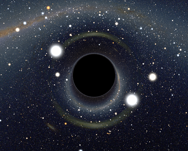
Figure 2: A example of an image computed using the methods outlined above, using the false color 2MASS full sky starless picture as well as the Henry Draper catalogue of stars. The black hole is put in front of the Large Magellanic Cloud, and specifically aligned with a 7.5 mag star (HD 49359) which is strongly lensed and appears as a two stars at equal distance but opposite position with respect to the black hole.

VII Adapting simulations for planetariums

In addition to their obvious mathematical/physical interest, an obvious use of astronomical simulations is for popular science shows, especially for planetarium since those are since more than a decade built upon a fully digital projection system. Since special and general relativistic effects are more spectacular close to the black hole horizon, which is therefore sustained by a large angular diameter, hemispherical projection are most naturally adapted to full-dome projection. For the purpose, we need to provide still frame or movies using the image format that is widely used in this field, the Domemaster format. Those are high definition (typically 4k$\times$4k, or even 8k$\times$8k square images whose largest incircle correspond to a half sphere. pixel distance with respect to the center of the image is proportional to colatitude and angle between a given ray and a downward half-line starting from the center of the square represent latitude. The pixel that lies at the middle of the inferior side of the square is in front of the audience and the pixel in the middle of the upper side of the square in behind it. Although the audience can look at any point of the planetarium screen, the most comfortable part to look at extends till around 60 degrees away from point of $60^{\circ}$ colatitude and $0^{\circ}$ longitude.

Regarding the rendering of the celestial sphere explained in§IV, the procedure here is exactly the same, except that Eqns (2, 3) have to be changed according to the above description of the Domemaster format, which amounts to change the relation between the pixel distance from the center of the screen to a given pixel with the angular separation between their associated directions (i.e., $Z^{\mu}$ and $N^{\mu}$ with the notations defined above). Those two equations are therefore rewritten as

$$i = \frac{S+1}{2}-\frac{S}{\pi}\frac{\theta}{\sin\theta}X_{\mu}N^{\mu},$$ (88)

$$j = \frac{S+1}{2}-\frac{S}{\pi}\frac{\theta}{\sin\theta}Y_{\mu}N^{\mu},$$ (89)

where $S$ is the number of pixel of any side of the square image (typically 4000 or 8000), and $\theta$ is the angle between $N^{\mu}$ and $Z^{\mu}$, i.e., $\theta=\arccos(-N_{\mu}Z^{\mu})$. Note that this transform does not only work for pixels belonging to the square incircle, but to all the pixels of the square image. Inverse transform follows immediately from Eqns (88–89).

Drawing the stars involves a slightly tweak with respect to §V an more specifically §V.3. This time, we want that the star appears as a circular blob with respect to the sky coordinates and not the pixel coordinates of the picture. Therefore, we proceed using a supplementary step:

1. From the star overall luminosity computed including the Doppler, amplification and lensing effect described above, we define the angular size of the blob that represents the star, after having chosen a normalization for this (i.e., a 1^stmagnitude star is represented by a blob of given angular size).

2. Then, we compute the position of the star in pixel space as before.

3. Further, we focus on the square region in pixel space centered on the star position and including all the pixels with angular separation (in real space) smaller than the assumed star size.

4. Finally, for each of the pixels in this region, we compute the angular separation (in real space) between the pixel center and the star position, and we draw the star according to its luminosity profile we have chosen (truncated Gaussian, or whatever else).

When looking at picture on a flat screen, stars will appear as elongated orthogonally to the radial direction, but when projected into a planetarium, they will appear as a circular blobs for observers sitting close to the center of the hemisphere. Observers sitting closer to the edges of the planetarium will experience some distortions, but this is the case for any picture projected that way. An example of picture computed for planetarium is given in Fig. 3.

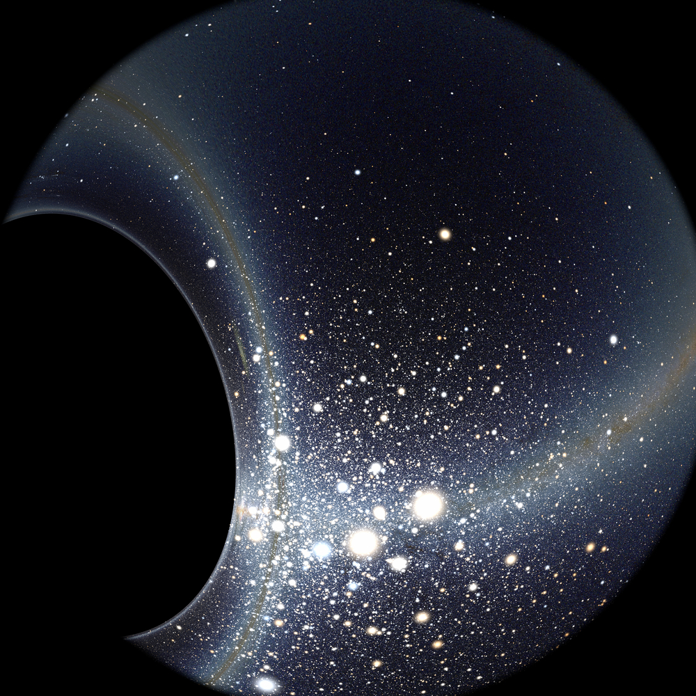
Figure 3: An example of a 4k$\times$4k picture computed for planetarium projection. It shows the view of an observer at the last stable orbit around a Schwarzschild black hole (i.e., $r=6M$), looking at the front direction, corresponding to 45 degrees above the horizontal edge of the planetarium, which here corresponds to the pixel (rounded down) $(2000,3000)$. The curious reader is encouraged to search for usually easy to recognize stars or constellations such as Ursa Major, Orion, $\alpha$ Boo, $\alpha$ Sco and $\alpha$ CMa, but it is quite involving due to the high velocity ($c/2$) causing significant luminosity and colour distortion to the familiar star background, as well as strong aberration and light deflection which severely affect the angular distance between stars.

VIII Delineating and crossing the horizon

As long as the observer lies outside the horizon, any calculation can be done in the standard Schwarzschild coordinates, although this is not necessarily what we do in practice. Such a coordinate choice is no longer possible when the observer is within the horizon since all the null geodesics he or she intersects have crossed the horizon and consequently have locally necessitated to use another coordinate system, see §III.2. However, apart from this, the procedure is the same: we compute the deflection function, and then we perform the drawing of the celestial sphere and of the stars.

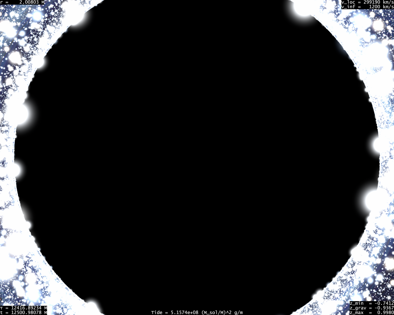
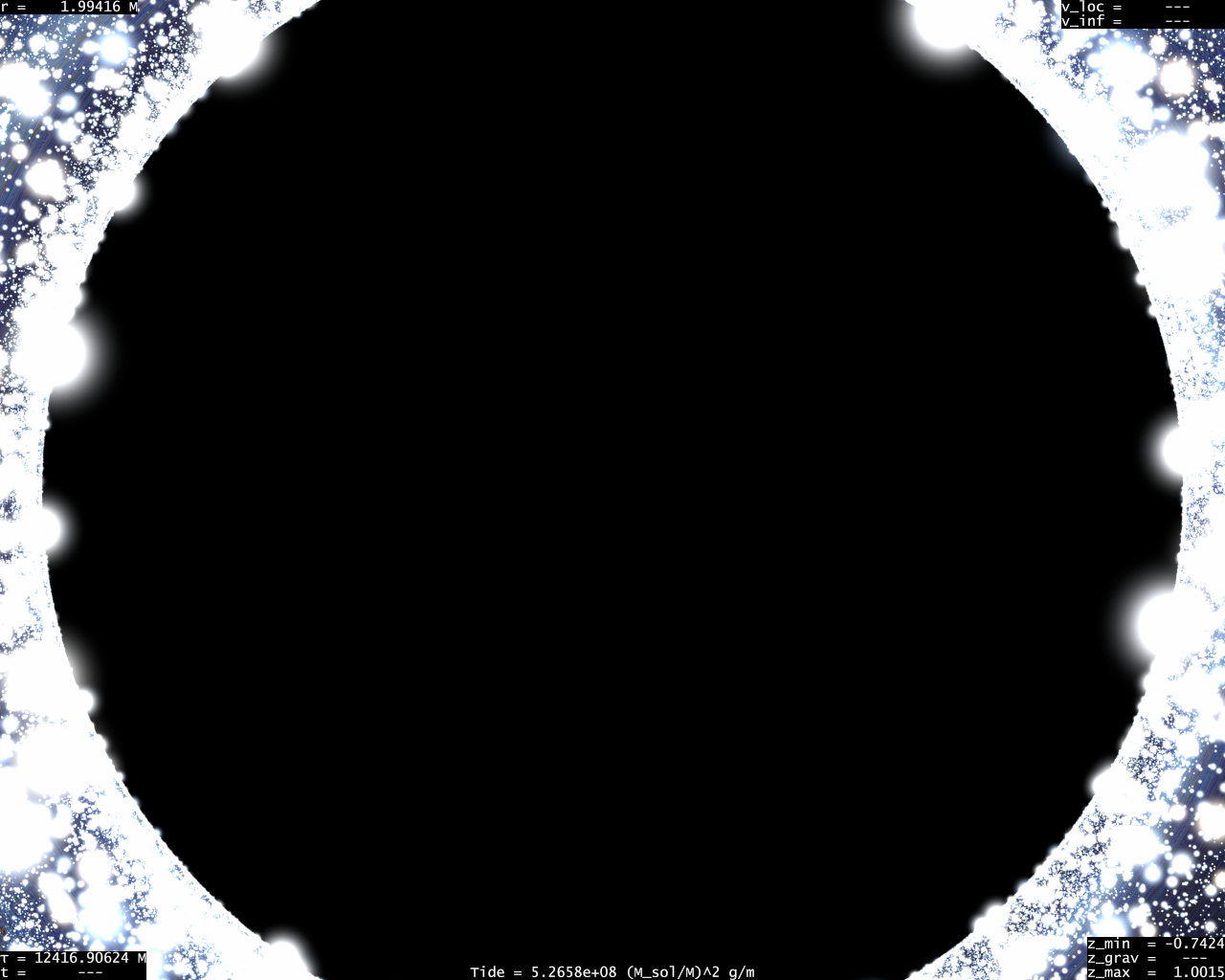
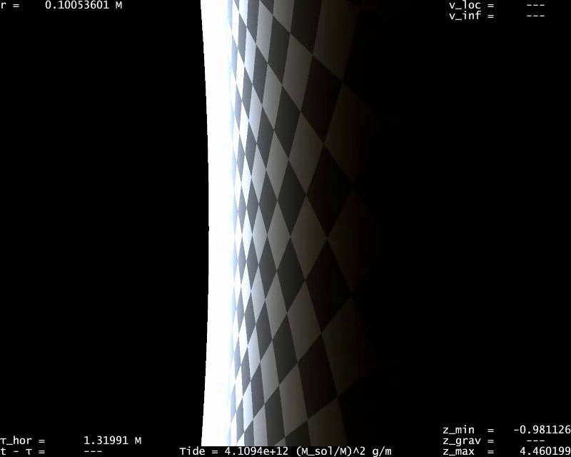
Figure 4: Three views of a radial geodesic trajectory plunging into the black hole. Top and middle image show the front view just before and just after horizon crossing. As expected, no visual hint allows to decide easily whether or not the observer has crossed the horizon. Bottom image shows the side view soon before hitting the singularity ($r\sim 0.1M$). We provide for this last picture a view with a coordinate grid only, so as to better emphasize the thinness of the blueshifted region. This representation also highlights that our celestial sphere grid, which lies at infinity, actually appears to be at decreasing, finite distance, falling on the observer.

We present in Fig. 4 three views of a radial geodesic trajectory starting from infinity and plunging into the black hole. Several interesting features seen in those images deserve an explanation:

• Firstly, if we consider the natural case of a freely falling observer with zero angular momentum and zero velocity at infinity (so that this observer’s velocity is $T_{\rm I}^{\mu}$), the angular size of the black hole is rather small at horizon crossing. This comes from the fact that an observer who is about to cross the horizon has a very large relative velocity with respect to a static observer close to the horizon. This means that the view seen by the former experiences a very strong aberration phenomenon with respect to the view seen by the latter, thus drastically reducing the black hole angular size. In order to determine the angular size of the black hole, one needs to consider a geodesic endowed with the critical impact parameter $|L/E|=3\sqrt{3}M$. As long as $r>3M$, the geodesic that delineates the horizon must have the above mentioned critical parameter, and must have almost reached the $r=3M$ region before bouncing back toward the observer. Therefore, it must be an outgoing geodesic, i.e., their $k^{r}$ component must be positive. For $r<3M$, the geodesics that start from null infinity and that reach the observer must be ingoing, i.e., their $k^{r}$ component must be negative. Without loss of generality, we can define a null geodesic under the form, following Eq. (76):

  $$k^{\mu}=\omega\left(T^{\mu}+\cos\delta R^{\mu}+\sin\delta\Theta^{\mu}\right),$$ (90)

  $\omega$ corresponding to the observed wavenumber of the associated wave. Without loss of generality, we can choose the $k^{\theta}$ component to be positive, so that $0\leq\delta\leq\pi$. Moreover, any geodesic starting for the observer’s initial region past null infinity must have a positive frequency, which amounts to say that

  $$\frac{E}{\omega}=1-\cos\delta\sqrt{2M/r}>0.$$ (91)

  This constraint is always true when $r>2M$, but has to be checked when $r<2M$, something we will address in the next Section. Finally, the $k^{r}$ component of the geodesic is

  $$k^{r}=\omega(\cos\delta-\sqrt{2M/r}).$$ (92)

  Therefore, following the previous discussion, we shall choose check that the sign of $k^{r}$ is compatible with the above criteria. These constraints being set, we need to compute the general solution of the equation $L/E=3\sqrt{3}M$ for the null geodesic we consider here. With the above definition of $k^{\mu}$, this amounts to solve equation

  $$\frac{r\sin\delta}{1-\sqrt{2M/r}\cos\delta}=3\sqrt{3}M.$$ (93)

  Defining $u\equiv r/M$ and solving the equation of the variable $\tan(\delta/2)$, we find

  $$\tan(\delta_{\eta}/2)=\frac{u+\eta\sqrt{u^{2}-27\left(1-\frac{2}{u}\right)}}{3\sqrt{3}\left(1+\sqrt{\frac{2}{u}}\right)},$$ (94)

  where $\eta=\pm 1$. The term within the square root in the numerator of Eq. (94) is bigger than $u$ when $u$ is smaller than $2$, so that the numerator is positive when $\eta>0$ whichever value of $u$, and is negative when $u<2$ and $\eta<0$. Regarding the denominator, it is always positive. Therefore, $\tan(\delta_{\eta}/2)$ is negative when both $u<2$ and $\eta<0$, so that this part of the solution must be discarded. Further, one can show (or check after plotting the functions as calculations are less straightforward) that the solution $\delta_{+}$ is not outgoing when $r>3M$ and are therefore excluded, and so is $\delta_{-}$ when $r<3M$ as it is not ingoing. Further, Eq. (91) is always valid for all remaining solutions, so that, taking into account the fact that the term under the upper square root of Eq. (94) can be factored by $(u-3)^{2}$, the allowed solution reduces to

  $$\tan(\delta/2)=\frac{u-(u-3)\sqrt{1+\frac{6}{u}}}{3\sqrt{3}(1+\sqrt{\frac{2}{u}})}.$$ (95)

  The physical interpretation of $\delta$ is simple. From an infalling observer point of view, a null geodesic of wavevector $k^{\mu}$ has an angular separation of $\delta$ with respect to the radial outgoing direction $R^{\mu}$. At horizon crossing, $u=2$ and

  $$\tan(\delta_{\rm hor}/2)=\frac{2}{3\sqrt{3}},$$ (96)

  so that

  $$\cos\delta_{\rm hor}=\frac{23}{31},$$ (97)

  leading to an angular diameter of the black hole silhouette of $2\arccos_{\rm hor}\delta\sim 84.2$ degrees. Such angular diameter would correspond, in Euclidean space, to that of a sphere seen at a altitude of $1/\sin\delta_{\rm hor}-1\sim 0,\!49$ times its radius. Coincidentally, such “altitude” in the Schwarzschild metric ($r=3M$) corresponds to that where a static observer sees the black hole silhouette encompass exactly the half of the celestial sphere, just as if one had landed on the perfectly dark surface, see middle part of Fig.20 in Appendix B.

• Secondly, soon before hitting the singularity, the same calculation gives the simple result

  $$\cos\delta_{\rm sing}=0,$$ (98)

  leading to an angular diameter of 180 degrees. In other words, hitting the singularity happens when the black hole silhouette fills exactly half of the celestial sphere, just as what would happen in a Euclidean space should one land on the surface of the spherical body.

• Thirdly, the celestial sphere is never very dark before horizon crossing. In order to see this, one simply has to notice that, as already stated, the scalar product $T_{\mu}k^{\mu}=\omega$ correspond to the observed wavenumber, whereas the constant of motion $E$ corresponds to the wavenumber measured by a static observer at infinity. Therefore, the shift between the observed and the initial frequency is

  $$\frac{1}{1+z}=\frac{\omega}{E}=\frac{1}{1-\cos\delta\sqrt{2M/r}}.$$ (99)

  The redshift therefore takes the simple expression

  $$z=-\cos\delta\sqrt{\frac{2M}{r}}.$$ (100)

  Whatever value of $r$ one considers, the maximum redshift is unsurprisingly obtained to radial ingoing radiation ($\delta=-\pi$, i.e., $\cos\delta=-1$ and is 1 at horizon crossing. The redshift of the radiation decreases to 0 in the orthogonal direction $\cos\delta=0$) and any direction closer to the black hole shows blueshifted radiation, the most blueshifted being the closest to the black hole silhouette, i.e., for $\delta=\delta_{\rm hor}$, for which $z=-23/31$.

  It is only when the observer is deep within the horizon that the maximum redshift significantly increases, taking the value $z=\sqrt{2M/r}$ for radial ingoing radiation. However, orthogonal directions still exhibit a zero redshift, but the region where redshift is moderate (between 0 and 1, say) becomes increasingly small as one approaches the singularity since it is bound to the shell of inner and outer radius $\pi/2$ and $\pi/2+\arcsin\sqrt{\frac{r}{2M}}$. The maximum blueshift is again obtain for the largest allowed value of $\cos\delta$, which is the one for which $L/E=3\sqrt{3}M$ The value of $\delta$ for which this holds tends to $\pi/2$, which allows to approximate Eq. (93) as

  $$3\sqrt{3}M\sim\frac{r}{1-\cos\delta\sqrt{\frac{2M}{r}}}=\frac{r}{1+z},$$ (101)

  which gives

  $$1+z_{\rm min}\sim\frac{r}{3\sqrt{3}M}.$$ (102)

  Therefore, soon before hitting the singularity, only a very thin ring of directions shows a blueshift, but the maximal blueshift diverges. Consequently, the last sight of the Universe seen by a freely falling observer is a very thin but also very bright ring of light, whose angular diameter is approximately $\pi$. Within this ring, everything is perfectly dark as it corresponds to the black hole silhouette, and outside this ring, the sky appears to be very dark, being highly redshifted.

IX Exploring the maximal analytic extension of the metric

IX.1 Looking at the other asymptotic region (region III)

From the Carter-Penrose diagram, it is obvious that an observer in region I cannot see anything of region III because the latter is not in the past lightcone of the former. The situation changes when the observer enters into region II because parts of both regions I and III are then in his/her past lightcone. A first obvious question one might ask is how this region looks like from such observer. For the sake of simplicity, we shall consider the simpler case of a freely-falling observer starting from region I with zero velocity at infinity.

The above framework can be adapted almost without much modification to the maximal extension of the metric. Indeed, once one is able to integrate backward a geodesic reaching an observer in region II and that had started from past null infinity of region I, there is no difficulty in doing so with geodesics originating from past null infinity of region III. Actually, any null geodesic that penetrates into region II can be cast under the form of Eq. (90), and it will originate from region III if two conditions are satisfied: (i) its constant of motion $E$ must be negative since in region III, $t$ is a past oriented timelike coordinate, so that $k^{t}={\rm d}t/{\rm d}p<0$, and, (ii) that its impact parameter $|L/E|$ is smaller than the critical value of $3\sqrt{3}M$ since this condition is always mandatory for a geodesics originating from past null infinity of any asymptotically flat region to be absorbed by the black hole. The edge of region III is therefore, as in the case of region I, delineated by geodesics of impact parameter equal to $3\sqrt{3}M$. We can, without loss of generality, impose that $L/E=3\sqrt{3}M$, which imposes to take $L<0$ since $E$ is negative. Therefore, this amount to solve the same equation as previously, but with $-\pi\leq\delta\leq 0$, for which one has $\tan\delta/2\leq 0$ and further take the opposite value of $\delta$ so as to recover the case where $0\leq\delta\leq\pi$. Following the previous discussion, this amounts to only consider the above part of the solution $-\delta_{-}$ when $u<2$, a result that makes sense since region III is seen only when one enters into region II. In the end, we have

$$\tan(\delta_{\rm III}/2)=\frac{1}{3\sqrt{3}}\frac{-u-(u-3)\sqrt{1+\frac{6}{u}}}{1+\sqrt{\frac{2}{u}}},$$ (103)

a value which ensures that, as requested, $\cos\delta_{\rm III}>\sqrt{u/2}$ whenever $u<2$. In order to check this, let us define $\cos\mu\equiv\sqrt{u/2}$. The requested inequality, $\cos\delta_{\rm III}>\sqrt{u/2}$, is equivalent to $\tan^{2}(\delta_{\rm III}/2)<\tan^{2}(\mu/2)$. Given the second order equation verified by $\tan^{2}(\delta_{\rm III}/2)$, we have $(1+\sqrt{2/u})\tan^{2}(\delta_{\rm III}/2)=\sqrt{2/u}-1-(2u/3\sqrt{3})\tan(\delta_{\rm III}/2)\geq\sqrt{2/u}-1$. But we have also $\tan^{2}(\mu/2)=(1-\cos\mu)/(1+\cos\mu)$, which is equivalent to $(1+\sqrt{2/u})\tan^{2}(\mu/2)=\sqrt{2/u}-1$, a value that is precisely the upper bound of $(1+\sqrt{2/u})\tan^{2}(\delta_{\rm III}/2)$, which completes the proof.

Now, when $\delta=0$, $L$ is also equal to $0$, so that region III correspond to any value of $\delta$ smaller than $\delta_{\rm III}$. The above equation immediately tells that $\tan(\delta_{\rm III}/2)=0$ at horizon crossing ($r=2M$), which amounts to say region III reduces to a single point when it becomes observable just after horizon crossing. Then, $\tan(\delta_{\rm III}/2)$ grows almost linearly as $r$ decreases (expanding the above relation gives $\delta_{\rm III}=3\sqrt{3}(2-u)/8+O((2-u)^{2})$ and reaches $1$ at $r=0$, which means that region III now encompasses a circular region of angular radius $\pi/2$. In other words, both regions I and III seem to join each other when the observer reaches the singularity, and the remaining part, which corresponds to geodesics originating from region II occupies a narrow shell which roughly is a great circle in the sky. The angular size of regions I and III are shown in Fig. 5.

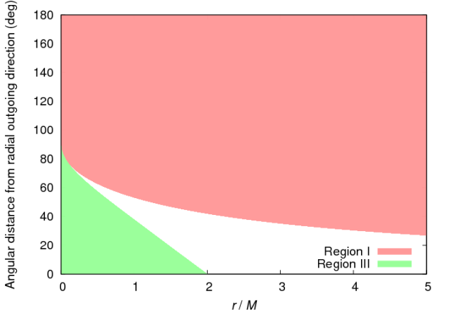
Figure 5: Diagram showing which of region I, III or black hole silhouette is seen as a function of angular separation between the front direction of a freely falling observer with zero velocity at infinity. Region I is always seen and decreases in size till it occupies half of the field of view at the singularity. Region III is, as expected, invisible outside the horizon and steadily grows afterward, till it reaches the half of the field of view. Black hole silhouette, or, in this context, geodesics originating from past singularity (region II) forms a shell between the two region, a shell that becomes infinitely thin as one approaches the singularity.

Within what is seen from region III the angular distortion have a similar behaviour to those of region I. The deflection function is zero in the front direction, and strongly increases as one approaches the edges of region III, leading to an infinity of closely packed multiple images of the celestial sphere. An example of the deflection functions of both region I and III is show in Fig. 6.

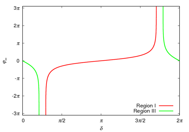
Figure 6: An example of both deviation functions $\varphi_{\infty}(\delta)$ of regions I and III as seen by an infalling observer at $r=M$. The server is still far, in term of coordinate distance, from the singularity, so that both regions have significantly different size, however, the deflection function are already quite similar.

An even less intuitive feature is how the redshift of region III evolves, both as a function of the angular distance to the central direction and of the coordinate distance. In this case, a slight difference arises with respect to null trajectories originating from region I. Indeed, if one assumes that a photon is sent from a static observer of four-velocity $u_{\rm stat,III}^{\mu}$ at past null infinity of region III, the photon wavenumber will be given by $\omega_{\rm III}=u_{\rm stat,III}^{\mu}g_{\mu\nu}k^{\nu}$. Assuming that this distant observer is static amounts to say that the only non zero component of its four-velocity is the time component, so that we have $\omega_{\rm III}=u_{\rm stat,III}^{t}E$. Moreover, since in region III, $t$ is a past-oriented timelike coordinate, $u_{\rm stat,III}^{t}=-1$, so that the wavenumber is

$$\omega_{\rm III}=-E.$$ (104)

Now, according to Eq. (90), $\omega$ corresponds to the observed wavenumber from the point of view of the infalling observer originating from region I, so that the frequency shift is $\omega/\omega_{\rm III}=\omega/(-E)$. Consequently, the redshift or blueshift of the radiation is given by

$$z=\cos\delta\sqrt{\frac{2M}{r}}-2.$$ (105)

If we consider first the ”front” direction $\delta=0$, there is an infinite blueshift at horizon crossing since $z=-1$. Further, when $r$ decreases, $z$ increases, becomes equal to 0 at $r=M/2$ and tends to infinity afterward, a situation that qualitatively mimics what happens for radial ingoing radiation coming from region I. Moreover, since $\cos\delta>0$, the redshift decreases as $\delta$ grows, so that region III appears as a disk whose center is dimmer than the edge. The center of the disk has a diverging redshift as $r$ goes to 0, whereas its edge experiences a blueshift, which, when $\delta_{\rm III}$ approaches $\pi/2$ approaches $1+z\sim u/3\sqrt{3}$, a value that, again, matches what the same observer sees with region I (see Eq. 102).

It might seem unexpected that regions I and III are seen almost identically from an infalling observer originating from region I, however, there is a rather simple explanation to this. First, what we have found here is identical to what a freely falling observer from region III would see, after exchanging in our results region I and region III. If we note by $T^{\mu}_{\rm III}$ this new freely falling observer’s velocity, then $T^{\mu}_{\rm III}$ has the same components as $T^{\mu}_{\rm I}$ except for the $t$ one, which is of opposite sign since $t$ is a past directed timelike coordinate in region III. Consequently, the dot product between the two infalling observers is

$$T^{\rm I}_{\mu}T^{\mu}_{\rm III}=\frac{\frac{2M}{r}+1}{\frac{2M}{r}-1}.$$ (106)

This quantity can be seen as the Lorentz factor of a boost one must perform to go from one velocity to the other. This Lorentz factor is infinite at horizon crossing. This explains why region III appears infinitely blueshifted from the point of view of observer $T^{\mu}_{\rm I}$, whereas is it moderately redshifted for observer $T^{\mu}_{\rm III}$ (such observer sees region III at horizon crossing exactly the same way observer $T^{\mu}_{\rm I}$ sees his own region I at horizon crossing). Now, as both observers move ahead within the horizon, their relative Lorenz factor decreases toward 1, which means that the two observers have a more and more similar perception of the two regions. Consequently, region III seen by observer $T^{\mu}_{\rm I}$ is very similar to the same region seen by observer $T^{\mu}_{\rm III}$, which by definition is seen in the same way as region I by observer $T^{\mu}_{\rm I}$, which explains why the two regions look more and more identical by this observer, as exemplified in Fig. 7.

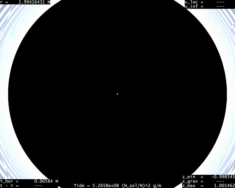
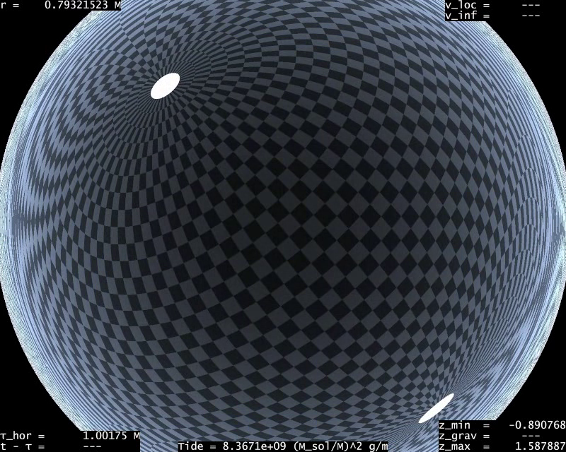
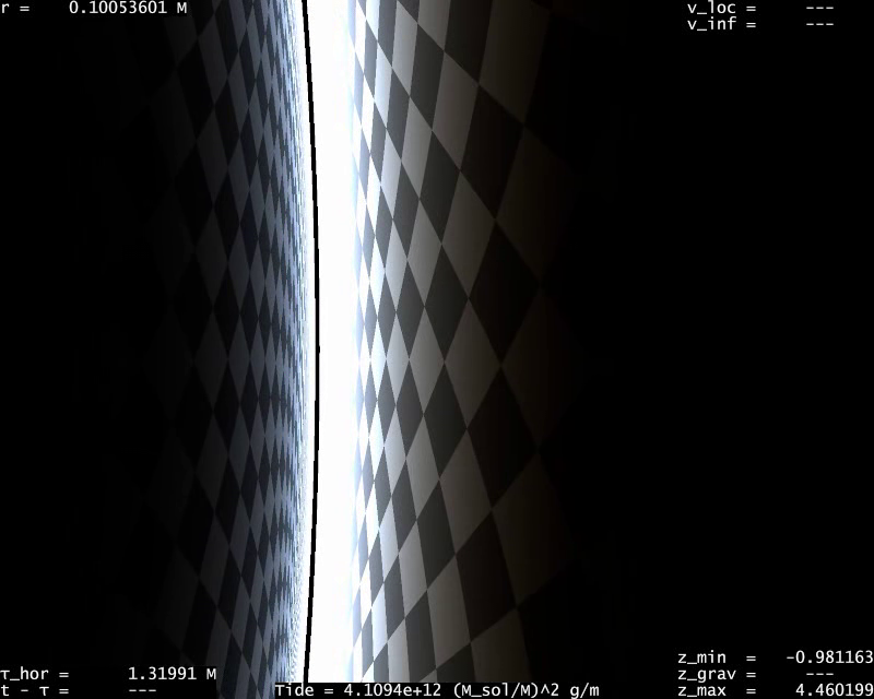
Figure 7: Three views of the maximal analytic extension of the metric. Top view shows the appearance of region III just after horizon crossing ($r\sim 1.994M$). Region I and region III look very different, as region III is an almost pointlike, infinitely blueshifted point, whereas region I, that surrounds the silhouette of the black hole is of large but finite blueshift on its edge and moderate redshift in its center (behind observer, not shown). Middle image show the view of region III at $r\sim 0.8M$, where darkening of central part of region III is visible, whereas its edge are blueshifted. Bottom image is a side view seen by an infalling observer close to the singularity ($r\sim 0.1M$). Region I, from which the observer originates, is on the right, and is identical with bottom view of Fig. 4, whereas region III is on the left. These two regions appear more and more identical as the observer approaches the singularity (see text). Celestial spheres of both regions were taken to be a coordinate grid so as to better illustrate the fact that they look more and more the same (in term of distortion) as the observer is moved toward future singularity.

So far, regions I and III are seen in an asymmetric way since we dealt with a freely falling observer coming from one of those regions. A natural question that arises is what happens in the most symmetric case, that is when the $t$ component of the observer four-velocity is 0 once in region II. This amount to consider an observer in region II with a four-velocity given by

$$T_{\rm II}^{\mu}=\left(\begin{array}[]{c}0\\ -\sqrt{\frac{2M}{r}-1}\\ 0\\ 0\end{array}\right).$$ (107)

We then consider the tetrad with this four-vector, the vectors $\Theta^{\mu}$ and $\Phi^{\mu}$ already defined in Eq. (25) and the “radial” vector

$$R_{\rm II}^{\mu}=\left(\begin{array}[]{c}\frac{1}{\sqrt{\frac{2M}{r}-1}}\\ 0\\ 0\\ 0\end{array}\right).$$ (108)

We can, as before, define a null vector crossing this new observer’s worldline as $k^{\mu}=\omega(T^{\mu}_{\rm II}+\cos\delta R^{\mu}_{\rm II}+\sin\delta\Theta^{\mu}$. $\delta=0,\pi$ correspond to the radial null trajectories originating from regions I and III, respectively. The most off-radial null trajectories originating from those two regions are those of impact parameter $3\sqrt{3}M$ which correspond to an angle given by

$$\frac{u\tan\delta}{\sqrt{\frac{2}{u}-1}}=3\sqrt{3}.$$ (109)

Therefore, at the edge of region II (i.e., $r$ close to $2M$), both regions I and III appear as a point whose redshift is given by $1/(1+z)=1/(\sqrt{2M/r-1}|\cos\delta|)$, i.e., an infinite blueshift. Further, as this observer goes toward the singularity, both regions I and III experience the same behaviour as previously described for infalling observers from regions I and III.

IX.2 Looking at the “white hole” (region IV)

IX.2.1 From outside the horizon

When considering the maximal analytic extension of the Schwarzschild metric, one usually assumes that nothing emerges from the past singularity, however, nothing prevents from computing geodesics originating from it and map what an observer can see from this singularity. Since there are no bound null geodesics, an observer will cross either (i) null geodesics originating from past null infinity of either his/her own region (if the observer is outside the horizon), or from any of the two asymptotic regions (if the observer has entered into the black hole), or (ii) null geodesics originating from the past singularity, i.e, region IV. If we want to include such geodesics, we simply need to assume that the past singularity emits some light whose spectrum depends on both the direction $\theta,\varphi$ and the there spacelike coordinate $t$.

If one neglects the $t$ dependence of the outgoing radiation, it is rather easy to guess what an observer would see outside the past horizon. Assuming an observer whose four-velocity is only along the radial direction (i.e. it is equal to $T^{\mu}_{\rm I}$), the outgoing radial null geodesic does not experience any deflection since it has zero angular momentum. Therefore, this direction of the white hole shows the radiation emitted from the same $\theta$ and $\varphi$ as the observer lies. Conversely, close to the edge of the white hole, when outgoing radiation has an impact parameter (measured at future null infinity almost equal to, although smaller than $3\sqrt{3}M$), the outgoing radiation experienced an arbitrarily large deflection, and the deflection decreases with the impact parameter. Consequently, the observer will see a series of copy of the white hole emission region, or, if one considers the $t$ dependence of the emission, a series of rings of variable $t$. The deflection function together with a view of the white hole region seen from an observer at $r=20M$ are shown in Figs 8–9.

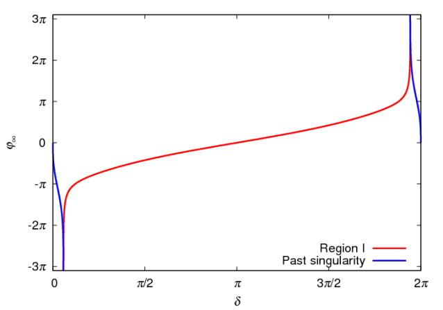
Figure 8: An example of all deviation functions of region IV (as well as I) seen from an observer outside the black hole, at $r=20M$. As explained in the text, there is an infinity of Einstein rings in what is seen of region IV. Also, because the black hole silhouette is seen from far, the deviation function is rather steep.

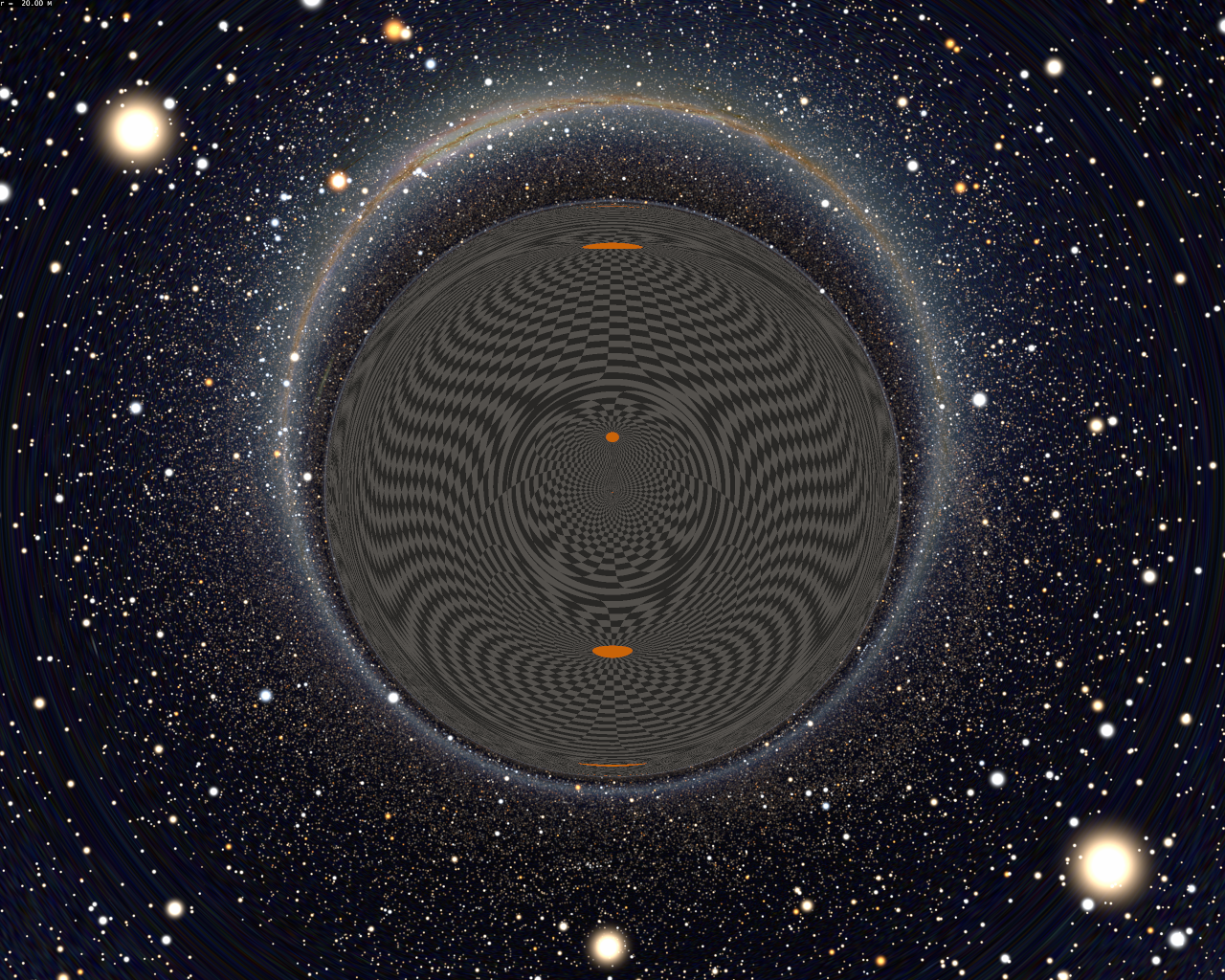
Figure 9: A view of the white hole region seen from a static standard, observer at $r=20M$. Observer’s asymptotic region is chosen to show the Milky Way, whereas white hole “celestial sphere” is chosen to be a coordinate grid (i.e., we do not assume any dependence with respect with the $t$ coordinate). We also removed any redshift information from this region. The “multiple images” in the white hole region are seen through the multiple views of the polar cap of the coordinate system. Note that since the deflection function is rather steep for close to radial outgoing trajectories, the coordinate grid in the center of the black hole silhouette is significantly shrunk.

IX.2.2 From the future horizon (region II)

If one then considers an observer that has entered the future horizon, then both regions I, III and IV are visible. Region IV fills the empty space that existed between the two asymptotic regions. The deviation function of region IV behaves differently as compared to the previous case. The reason is that outside the horizon, the observer can spot the purely radial outgoing null geodesic. This is not possible within the future horizon as the observer cannot intersect this geodesic any longer. Therefore, any geodesic originating from region IV reaching region II is non radial and has experienced some amount of deviation. Consequently, the deviation function has a local extremum. On the edge of its domain of definition, the deviation function still diverges as it corresponds to geodesics which have exited the past horizon (either entering into region I or III and which then bounced back at $r=3M^{-}$ after having experienced an arbitrarily large deviation. An example of the deviation function is shown in Fig. 10 and the corresponding view is shown in Fig. 11.

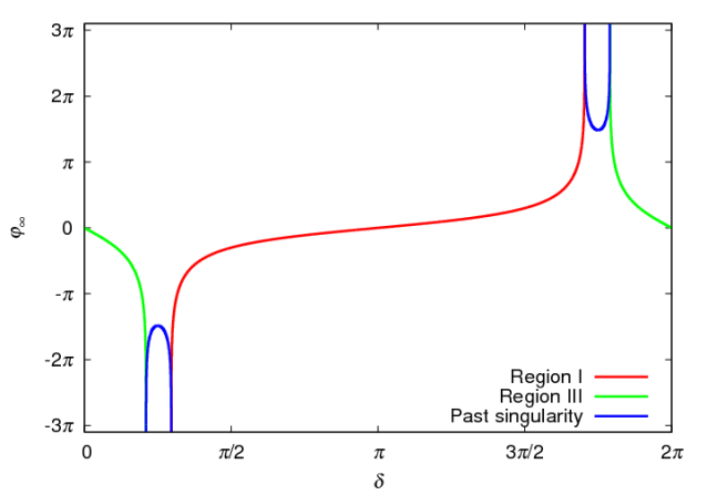
Figure 10: An example of all deviation functions in the complete analytic extension of the metric, assuming that something emerges from the past singularity. As in Fig 6, the observer is situated at $r=M$.

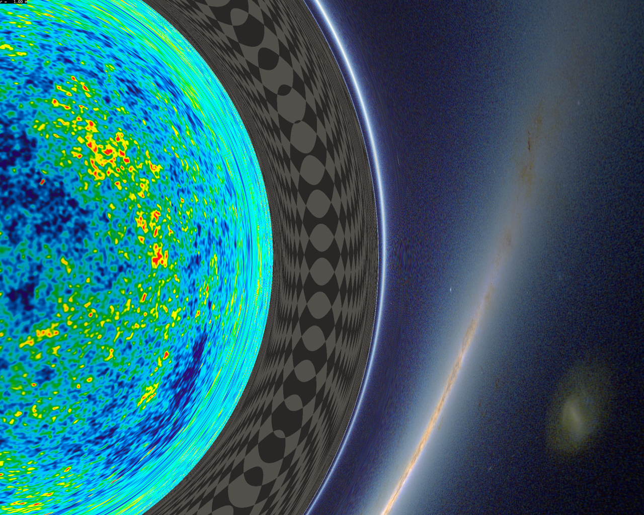
Figure 11: A view of the white hole region seen from an infalling observer at $r=M$. The view is $45\circ$ away from radial direction. As for previous image, region I, to the right, shows the Milky Way, whereas region III, on the left shows (rather arbitrarily) a CMB map.

*** DIRE PLUS

IX.2.3 From the past horizon

Another question one may want to address is what happens in the (rather academic) case of a very hypothetical observer originating from the past singularity and still in region IV. In this case, any direction of observation shows null geodesics originating from the past singularity since none of the other regions of the Kruskal extension are in such an observer’s past lightcone. Very close to the singularity, so that we can keep only the leading terms in $1/r^{n}$ in Eq. (120), a null geodesics follows the simplified equation

$$\left(\frac{{\rm d}r}{{\rm d}p}\right)^{2}\simeq\frac{2ML^{2}}{r^{3}},$$ (110)

where $p$ is an affine parameter of the geodesic. This amounts to say that $r$ initially varies as $p^{\frac{2}{5}}$. From the constancy of $L=r^{2}{\rm d}\theta/{\rm d}p$, we have $\theta-\theta_{0}\propto p^{\frac{1}{5}}$, and applying the same procedure with the other constant of motion $E$, we have $t-t_{0}\propto p^{\frac{7}{5}}$, where in both cases the $0$ subscripts denote quantities evaluated at the beginning of the geodesic. Therefore, an observer close to the singularity will have a past light cone that intersect only a small portion of the singularity, both in term of the angular and “time” dependence.

In order to use our formalism in the region, we need to redefine vectors $T^{\mu}$ and $R^{\mu}$, whose most natural choice is then

$$T_{\rm IV}^{\mu}=\left(\begin{array}[]{c}0\\ \sqrt{\frac{2M}{r}-1}\\ 0\\ 0\end{array}\right)\qquad,\qquad R_{\rm IV}^{\mu}=\left(\begin{array}[]{c}\frac{1}{\sqrt{\frac{2M}{r}-1}}\\ 0\\ 0\\ 0\end{array}\right).$$ (111)

We then consider the tetrad with this four-vectors, as well as the four-vectors $\Theta^{\mu}$ and $\Phi$. As before, we shall consider a hypothetical observer with four-velocity $T_{\rm IV}^{\mu}$, and consider null geodesics of four-wavevector $k^{\mu}$ defined in Eqns. (76,90) crossing his/her worldline

The amount of deflecting experienced by a null geodesic between the singularity and an observer at some $r_{\rm obs}<2M$ is given by the formula

$$\Delta\varphi=\int_{0}^{r_{\rm obs}}\frac{L{\rm d}r}{r^{2}\sqrt{E^{2}+\left(\frac{2M}{r}-1\right)\frac{L^{2}}{r^{2}}}},$$ (112)

where $E$ and $L$ are the null geodesics associated constants of motion. Setting $u=r/M$ and defining the dimensionless impact parameter $\bar{b}=L/EM$, we have

$$\Delta\varphi={\rm sgn}(L)\int_{0}^{u_{\rm obs}}\frac{{\rm d}u}{\sqrt{\frac{u^{4}}{\bar{b}^{2}}+2u-u^{2}}}.$$ (113)

When $\bar{b}=0$, i.e., a radial trajectory (or what will become so after exiting the horizon, the deflection is 0, and the absolute value of the deflection grows as $\bar{b}$ grows since the denominator in the integral is a decreasing function of $\bar{b}$. For an infinite value of $\bar{b}$, which corresponds to a trajectory whose ${\rm d}t/{\rm d}p=0$, the above equation reduces to

$$\Delta\varphi={\rm sgn}(L)\int_{0}^{u_{\rm obs}}\frac{{\rm d}u}{\sqrt{2u-u^{2}}},$$ (114)

whose solution is

$$\Delta\varphi={\rm sgn}(L)\left(\arcsin(u_{\rm obs}-1)+\frac{\pi}{2}\right),$$ (115)

a value which tends to $\pm\pi$ as $r$ approaches $2M$. Now, the relation between the viewing angle $\delta$ and the reduced impact parameter $\bar{b}$ is, given our definitions of $T_{\rm IV}^{\mu}$ and $R_{\rm IV}^{\mu}$ in Eq. (111), given by

$$\bar{b}=\frac{L}{EM}=\frac{u}{\tan\delta\sqrt{\frac{2}{u}-1}}.$$ (116)

For fixed $\tan\delta$, and hence a fixed observing direction, the associated impact parameter decreases toward zero as $r$ approaches $2M$, so that the observer sees geodesics originating from almost the same $\theta$ and $\varphi$ he/she is situated at, regardless on which direction he/she is looking at. From a visual point of view, this translates into the (rather unusual) features:

1. Very near the singularity ($r\ll 2M$), the observer sees only a small patch of the singularity, something that is intuitive.

2. Far less intuitively, as $r$ grows, a large part of the field of view is occupied by neighbouring parts of the singularity, whereas two opposite direction ($\pm\partial/\partial t$) show a rapid variation of the region of the singularity that is seen. Along these two directions, the visual aspect of the angular coordinate grids looks like as if we had projected a sphere along a more and more elongated funnel.

3. When $r\lesssim 2M$, almost all directions of observation show the same angular part of the singularity, and only two opposite directions show all the rest of the angular part of the singularity, which is confined within a decreasing angular size.

Four examples of deviation functions together with the corresponding views are shown in Figs. 13,13.

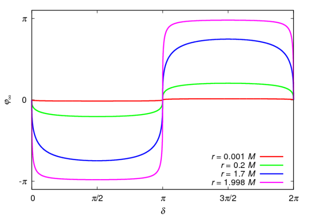
Figure 12: Deviation function for region IV seen from region IV for four values of $r$. As explained in the text the deviation function tends to a step function as $r$ approaches $2M$, which translates into the confusing visual aspect of next Figure.

Figure 13: Set of views of region IV by an observer in region IV. The four fisheye view are taken at $r=0.001M$, $r=0.2M$, $r=1.7M$ and $r=1.998M$ and toward the same direction. When the observer ”takes off” from the singularity, only a narrow part of it is seen (bottom left picture). Further, when ^′ increases, the view of the singularity seems to become more and more elongated along the $\pm\partial/\partial t$ direction (opposite view is essentially identical to the one shown).

Of course, of choice of the observer’s four-velocity $T_{\rm IV}^{\mu}$ is somewhat questionable because such observer’s trajectory is the only one that does does not exit to horizon, as it directly goes from region IV to region II when when its trajectory reaches its “apex”, at $r=2M$. One may prefer to consider instead an analog of our freely-falling observer $T_{\rm I}^{\mu}$, except that we want that this new observer originates from the past horizon (and, hence, the past singularity) instead of heading toward its future counterpart. This amounts to change the $T_{\rm I}^{\mu}$ of Eq. (16) into

$$T_{\rm I^{\prime}}^{\mu}=\left(\begin{array}[]{c}\frac{1}{1-\frac{2}{u}}\\ +\sqrt{\frac{2}{u}}\\ 0\end{array}\right).$$ (117)

The scalar product between $T_{\rm I^{\prime}}^{\mu}$ and $T_{\rm IV}^{\mu}$ gives

$$T_{\rm I^{\prime}}^{\mu}T_{{\rm IV},\mu}=\frac{1}{\sqrt{1-\frac{u}{2}}},$$ (118)

which means that the two observers have a larger and larger relative velocity (equal to $\sqrt{u/2}$). Therefore the views seen by observer endowed with four-velocity $T_{\rm IV}^{\mu}$ and $T_{\rm I^{\prime}}^{\mu}$ become more and more different because of aberration (and also Doppler shift, which we do not show in the views of region IV). An example of this is shown in Figure 14, to be compared to the bottom row of Fig. 13.

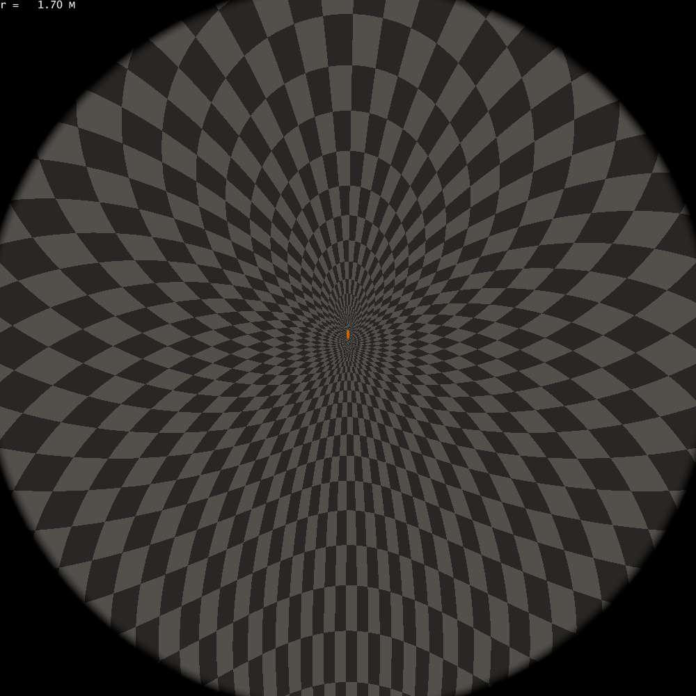
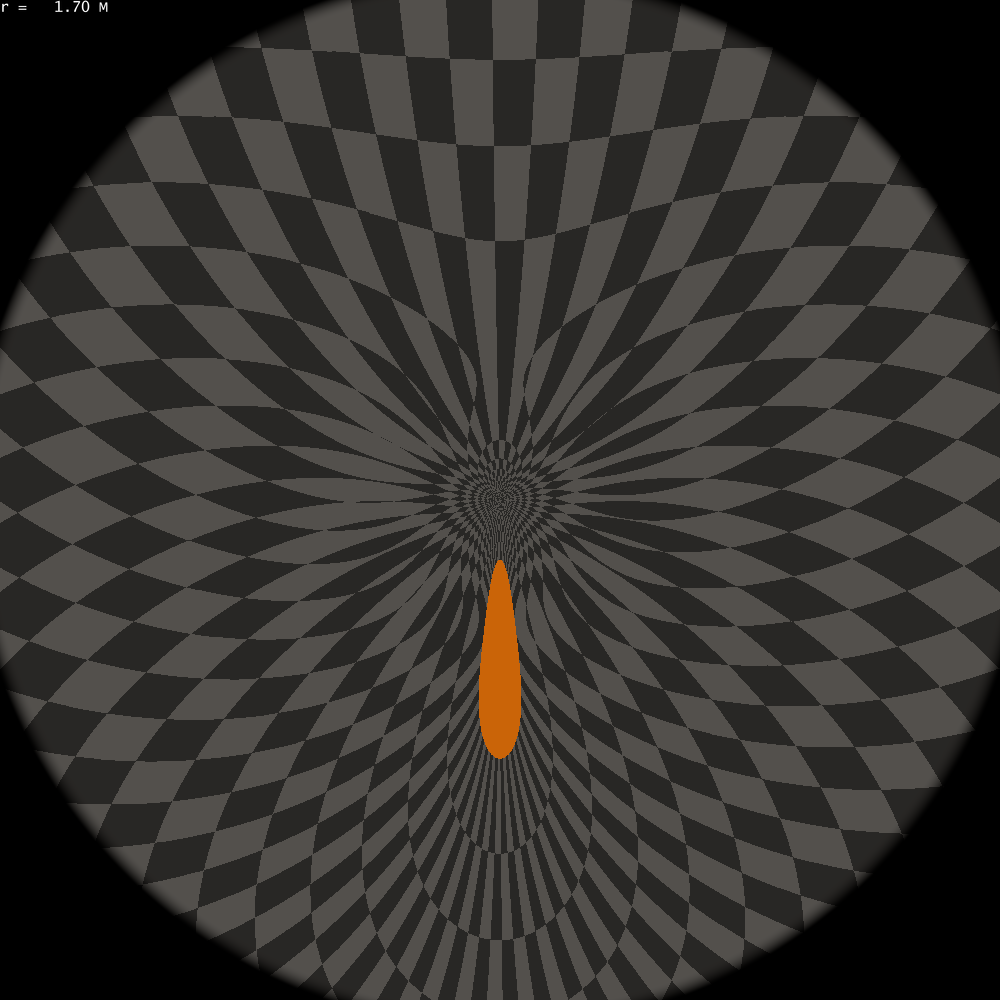
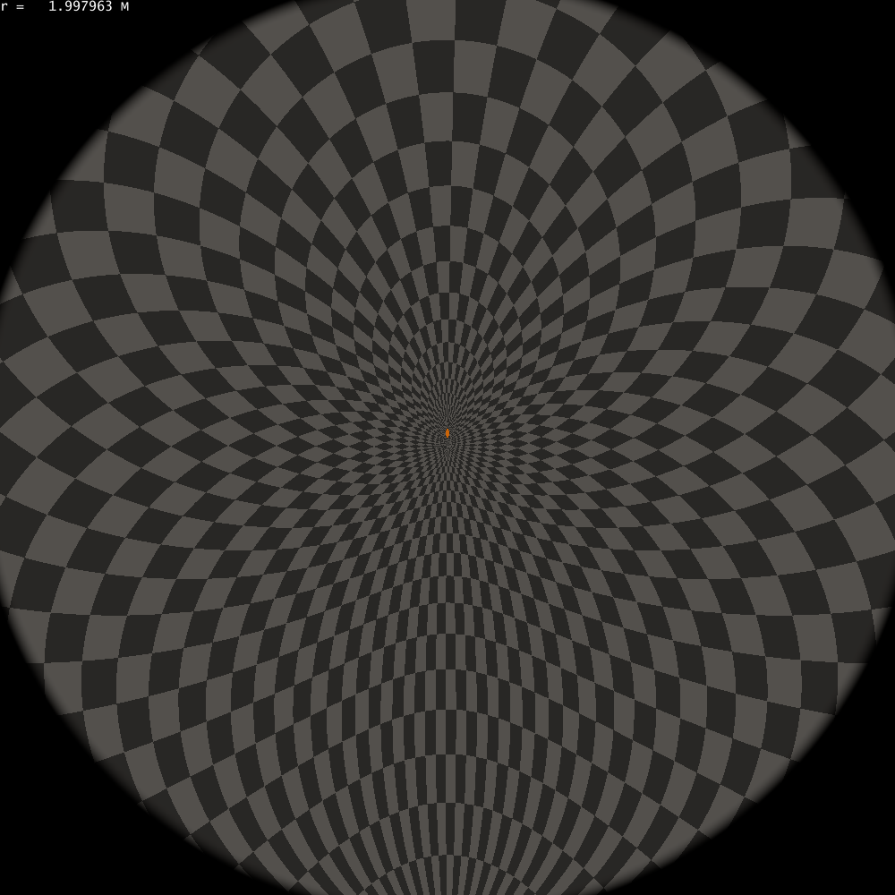
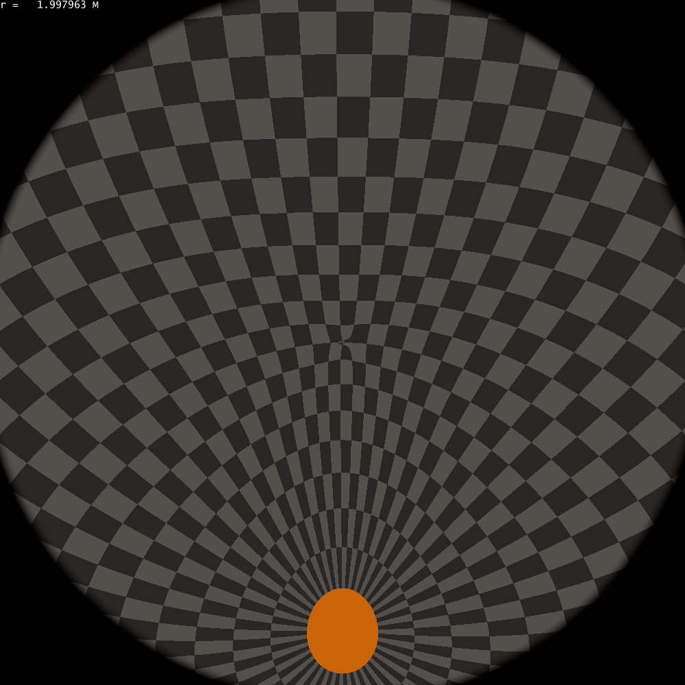
Figure 14: Front (right) and rear (left) views at $r=1.7M$ (top) and $r=1.998M$ (bottom) by an observer about to exit region IV to reach region I and who will then become a ZAMO outgoing observer with zero velocity at infinity. The front view is to be compared with the bottom row of Fig. 13: the field of view is significantly shrunk. The transition between the two is reasonably obvious for $r=1.7M$, as one can follow the displacement of the orange spot toward the center of the view. However, for $r=1.998M$ the view, that was already significantly shrunk toward the middle, is so much shrunk again whereas is the same time the rear view completely unfolds and encompasses the front view, so that one may think that there is only a minor distortion at the very center of the front view.

X Conclusion

In this paper, we have outlined the main steps in order to produce a correct rendering of relativistic ray tracing in the Schwarzschild metric. Although this problem is not new, we have obtained a very satisfactory (and, to our knowledge, new) way to simulate correctly the rendering of stars without any significant increase of the CPU time. This was made possible thanks to the spherically symmetric character of the Schwarzschild metric. This method does not rely on the specific projection scheme one adopts for the viewing screen and is therefore very well adapted for digital planetarium hemispheric projection.

One major drawback of the techniques presented here is that they are still computationally intensive and do not allow real-time rendering of the metric since even at moderate resolutions, the CPU time is of several dozens of seconds. Real-time rendering thus necessitates to reduce CPU time by a factor greater than $10^{3}$, which is a rather ambitious goal, the attainability of which will be presented in a future work.

Using these techniques, we performed a thorough exploration of the Schwarzschild metric. Many results were already known, but we found several novel effects when exploring the visual aspect beyond the horizon, and more specifically when considering the maximal analytic extension of the metric, i.e., the Kruskal-Szekeres extension. In particular, we found that when one visualizes the other asymptotic region, it appears at first infinitely blueshifted when the observer crosses the horizon and starts seeing it, but further, it is increasingly redshifted, except on its edges which are blueshifted. Also, we studied the case of an observer originating from the past singularity of the metric and who witnesses very unusual visual effects, assuming that radiation originates also from the singularity.

A natural follow-up of this work is to implement other spherically symmetric metric, the most natural of which being the Reissner-Nordstrom one, some result of which will be presented elsewhere. Unfortunately, out fast ray tracing method is less suited for the Kerr metric or any other non spherically symmetric metric such as the Papapetrou-Majumdar one. Some results regarding these metrics will also be presented elsewhere.

Appendix A On the structure of null geodesics in the Schwarzschild metric

We briefly recall here the different types of null geodesics in the Schwarzschild metric as well as the parameters that allow to distinguish them.

A null geodesics described by wavevector $k^{\mu}$ is characterized by the trivial equation

$$g_{\mu\nu}k^{\mu}k^{\nu}=0.$$ (119)

Using the constants of motion $E$ and $L^{2}$ defined in Eqns (54,55), this can be rewritten

$$E^{2}-\dot{r}^{2}=\frac{L^{2}}{r^{2}}\left(1-\frac{2M}{r}\right),$$ (120)

where for simplicity $\dot{r}$ denotes the $r$ component of the wavevector.

Such an equation can formally be seen as describing the motion of a one dimensional particle along coordinate $r$, with a total energy $E^{2}/2$ and subject to a potential $V(r)$ given by

$$V(r)=\frac{1}{2}\frac{L^{2}}{r^{2}}\left(1-\frac{2M}{r}\right).$$ (121)

This potential goes to $0$ at infinity and tends to minus infinity when $r$ goes to $0$. It has a unique maximum at $r=3M$ (regardless of the value of $L^{2}$) whose value is $V_{\rm max}=L^{2}/54M^{2}$.

Consequently,

1. If $E^{2}/2>V_{\rm max}$, or, equivalently $|L/E|<3\sqrt{3}M$, then the geodesic does not have any turning points along the $r$ coordinate and therefore its endpoints are $r=0$ and $r=\infty$. It originates from infinity if and only if $\dot{r}<0$.

2. If $E^{2}/2<V_{\rm max}$ then the geodesics has its both endpoints either at $r=0$ or at $r=\infty$. In the first case, it always lies within the $[0,r_{\rm max}<3M]$ region and in the second case it always lies in the $[r_{\rm min}>3M,\infty[$ region. The values of $r_{\rm max}$ and $r_{\rm min}$ are computed by finding the positive roots of the third degree polynomial equation $E^{2}/2=V(r)$, the solution of which can be expressed in term of moderately simple elementary functions which do not matter here since if one has $E^{2}/2<V_{\rm max}$) a geodesic originates from infinity if and only if one lies at $r>3M$.

3. The critical case $|L/E|=3\sqrt{3}M$ corresponds to geodesics which are stuck at $r=3M$ or which indefinitely spiral toward this value, either originating from $r=0$ of from $r=\infty$. In practice such geodesics never have to be taken care of since numerical round-off error prevent from having this exact value of the $L/E$ ratio even if one tries to.

Moreover, the ratio $|L/E|$ can be interpreted as some apparent impact parameter for the geodesic wald84 .

From the shape of the effective potential, it is easy to understand that if the observer is at $r>3M$, outgoing null geodesics that intersect his/her worldline can originate from past null infinity only if their impact parameter is larger than the critical value $b_{\rm crit}=3\sqrt{3}M$. From the observer’s point of view, there exists therefore a critical angle which separates outgoing geodesics with $b>b_{\rm crit}$ and $b<b_{\rm crit}$. The former originate from past null infinity whereas the latter originate from the black hole past horizon. Therefore, the deviation function $\varphi_{\infty}(\delta)$ is bounded for the $\delta$ corresponding to such outgoing geodesic with impact parameter larger than the critical value $b_{\rm crit}$. Moreover, outgoing null geodesics with an impact parameter close but above $b_{\rm crit}$ will experience a large deviation since, given the effective potential, the value of ${\rm d}\varphi/{\rm d}r$ is given by

$$\frac{{\rm d}\varphi}{{\rm d}r}=\frac{1}{r}\frac{1}{\sqrt{\frac{r^{2}}{b^{2}}-\left(1-\frac{2M}{r}\right)}},$$ (122)

a value which is very large when $r\sim 3M$, $b\sim b_{\rm crit}$, because then geodesics on the potential hill when its slope is very small. Consequently, geodesics which correspond to the edge of the domain of definition of $\varphi_{\infty}(\delta)$ experience a diverging deviation as shown in Fig. 1.

A similar reasoning also applies for an observer at $r<3M$ if we now consider ingoing geodesics with impact parameter close to but smaller than $b_{\rm crit}$.

Appendix B Some images

The methods that we have outlined can now be implemented to compute high quality images of black holes in various situations, and to explore the unexpected variety of special and general relativistic effects that one would visually experience close to a black hole. For pedagogical purpose, we shall try to isolate each of those effects one by one.

B.1 Special relativistic effects only

In this subsection, we shall consider Minkowski space only.

Let us assume an observer traveling at a constant velocity $\bm{v}$ with respect to a reference observer whose celestial sphere is well-defined. We note $(t,{\bm{x}})$ a set of Cartesian coordinates for the reference observer and $(t^{\prime},\bm{x}^{\prime})$ those of the second one. Up to some unimportant constant, the second set of coordinates is expressed in term of the first one as:

$$t^{\prime} = \gamma(t-\bm{x}\cdot\bm{v}),$$ (123)

$$\bm{x^{\prime}}_{\perp} = \bm{x}_{\perp},$$ (124)

$$\bm{x^{\prime}}_{\parallel} = \gamma(\bm{x}_{\parallel}-\bm{v}t),$$ (125)

where $\bm{x}_{\parallel}$ and $\bm{x}_{\perp}$ represent the parallel part and the perpendicular part of the spacelike coordinates with respect to velocity $\bm{v}$. As well-known, the last two equations can be rewritten into a single one:

$$\bm{x}^{\prime}=\bm{x}-\gamma\bm{v}t+\frac{\gamma^{2}}{\gamma+1}(\bm{v}\cdot\bm{x})\bm{v}.$$ (126)

The associated Lorentz transform can be seen as the matrix whose components are $\Lambda^{\mu}_{\;\nu}=\partial x^{\prime\mu}/\partial x^{\nu}$, which here can be written (see Eq. (6))

$$\Lambda^{\mu}_{\;\nu}=\left(\begin{array}[]{cc}\gamma&-\gamma\bm{v}\\ -\gamma\bm{v}&{\rm Id}+\frac{\gamma^{2}}{\gamma+1}\bm{v}\otimes\bm{v}\end{array}\right)$$ (127)

From the point of view of the reference observer, a wavevector $k^{\mu}$ associated to a direction $\bm{n}$ has components given by

$$k^{\mu}=\omega\left(\begin{array}[]{c}1\\ -\bm{n}\end{array}\right).$$ (128)

In the second observer frame, the wavevector has the new coordinates

$$k^{\prime\mu} = \Lambda^{\mu}_{\;\nu}k^{\nu}$$ (131)

$$= \omega\left(\begin{array}[]{c}\gamma(1+\bm{v}\cdot\bm{n})\\ -\bm{n}-\gamma\bm{v}\left(1+\frac{\gamma}{\gamma+1}(\bm{v}\cdot\bm{n})\right)\end{array}\right)$$

$$\equiv \omega^{\prime}\left(\begin{array}[]{c}1\\ -\bm{n}^{\prime}\end{array}\right).$$ (134)

The direction $\bm{n}^{\prime}$ and frequency $\omega^{\prime}$ of the corresponding photon seen from the second observer are therefore

$$\bm{n}^{\prime} = \frac{\bm{n}+\gamma\bm{v}\left(1+\frac{\gamma}{\gamma+1}(\bm{v}\cdot\bm{n})\right)}{\gamma(1+\bm{v}\cdot\bm{n})},$$ (135)

$$\omega^{\prime} = \omega\gamma(1+\bm{v}\cdot\bm{n}).$$ (136)

Although it is not obvious at first sight, the vector $\bm{n}^{\prime}$ has norm $1$ as expected.

B.1.1 Aberration

Aberration describes the way the spacelike components of a null vector are transformed during a Lorentz boost. Its main effect is that the angle between some star and the direction one is travelling to diminishes as velocity increases. Starting from Eq. (135) and denoting $\alpha$, $\alpha^{\prime}$ the angle between $\bm{n}$ and $\bm{v}$ on the one hand, and $\bm{n^{\prime}}$ and $\bm{v}$ on the other hand, one has

$$\cos\alpha^{\prime}=\frac{\cos\alpha+v}{1+v\cos\alpha},$$ (137)

so that, as expected,

$$\cos\alpha^{\prime}-\cos\alpha=\frac{v\sin^{2}\alpha}{1+v\cos\alpha}>0.$$ (138)

The relation between $\alpha$ and $\alpha^{\prime}$ can be inverted, either by direct algebra or by noticing that it suffices to change the sign of $v$ in order to make the inversion make sense, so that

$$\cos\alpha=\frac{\cos\alpha^{\prime}-v}{1-v\cos\alpha^{\prime}}.$$ (139)

A few examples of the aberration effect are shown in Figures 15,16.

Figure 15: Aberration seen by an observer starting from a static situation with respect to the celestial sphere (upper left image) to $v=0.3$ (upper right image), $v=0.6$ (lower left image), and $v=0.9$ (lower right image). In all the pictures the field of view is $90$ degrees along the horizontal direction. The “squares” delineating the celestial sphere are $5$ degrees wide both in latitude and longitude (see Section VI.1). Eq. (139) can be checked by visual inspection of the number of squares along the central horizontal band. The initial angular separation between the central part of the vertical edges of the images is $90$, $~{}117.8$, $158.6$, $244.1$ degrees, respectively. The two poles of the celestial sphere, which by definition are 180 degrees apart for a static observer are now, from Eq. (137), only $51.7$ degrees apart on the last image.

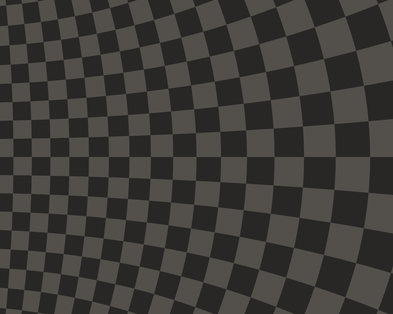
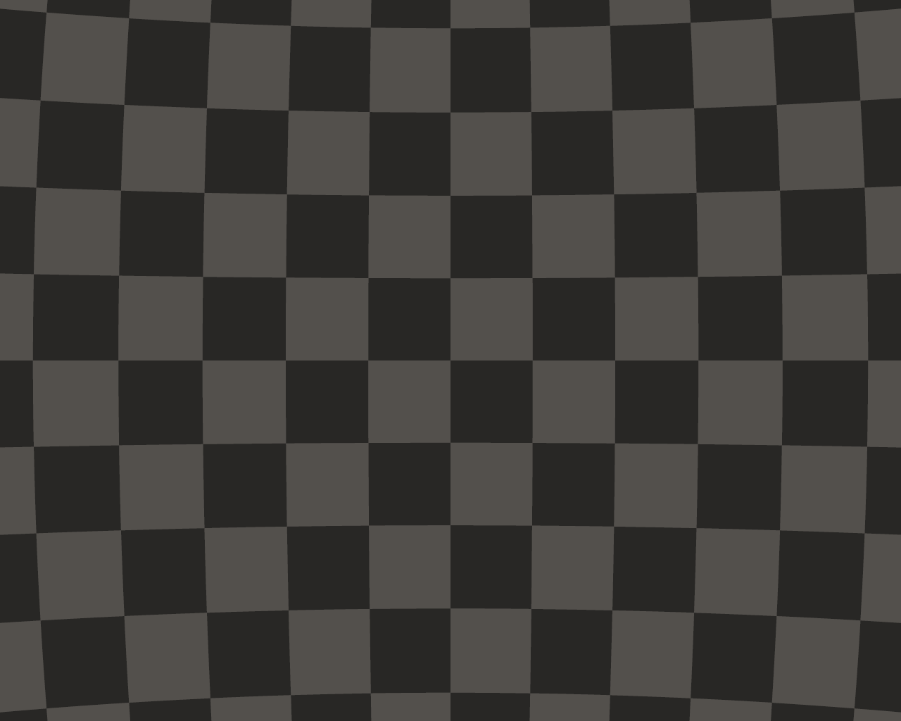
Figure 16: Aberration seen by an observer travelling at $v=0.5$ with respect to the frame where the celestial sphere is defined (see Sec. VI.1). Upper left image shows the front view, followed by the right view (upper right) and rear view (lower left). Without aberration, these three views should match the static one, in the lower right corner.

B.1.2 Doppler

The frequency shift $\omega^{\prime}$ given by Eq. (136) is more conveniently written in term of the angle $\alpha^{\prime}$ as it is the one that is actually observed. It reads

$$\omega^{\prime}=\frac{\omega}{\gamma(1-v\cos\alpha^{\prime})}.$$ (140)

One recovers the usual result that the frequency shift goes between $\sqrt{(1-v)/(1+v)}$ and $\sqrt{(1+v)/(1-v)}$ when going from the opposite direction to the direction of $\bm{v}$. Along the perpendicular direction (i.e., $\cos\alpha=0$), the frequency shift is $\gamma^{-1}$, i.e., there is an observed redshift. The region along which there is a blueshift if the one where $\omega^{\prime}>\omega$, which corresponds to

$$\cos\alpha^{\prime}>\frac{\gamma v}{\gamma+1},$$ (141)

which, in term of the angle $\alpha$ corresponds to

$$\cos\alpha>-\frac{\gamma}{\gamma+1}.$$ (142)

This means that when the velocity is large, the angular size of the blueshifted region is increasingly smaller (the lower bound on $\cos\alpha^{\prime}$ increases), but corresponds to an initially increasingly larger patch of the sky seen by the first observer (the lower bound on $\cos\alpha$ increases). An example of the observed color change due to the Doppler effect is shown in Fig. 17.

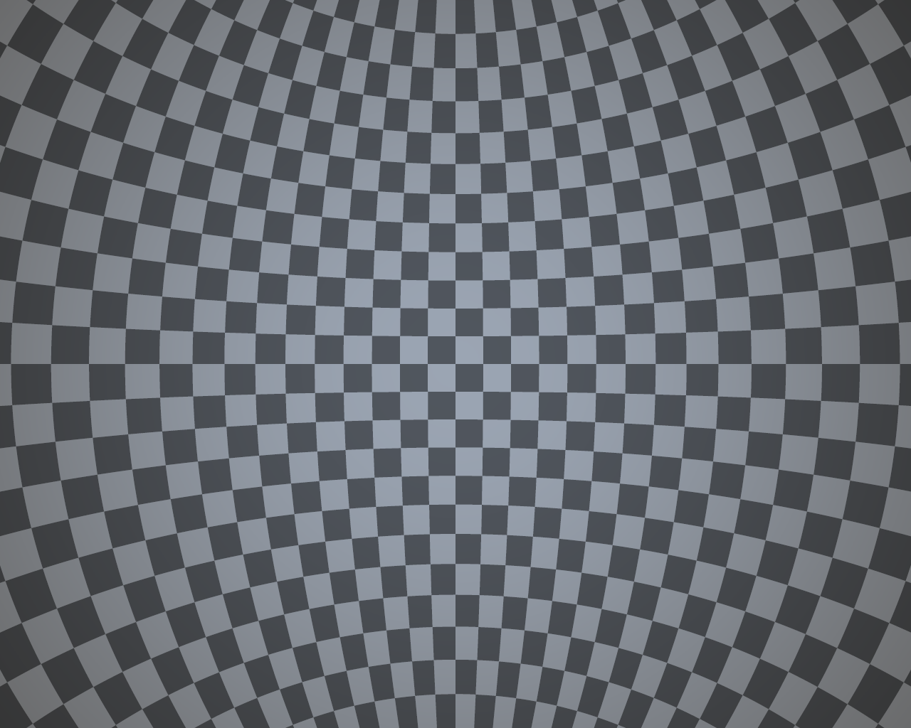
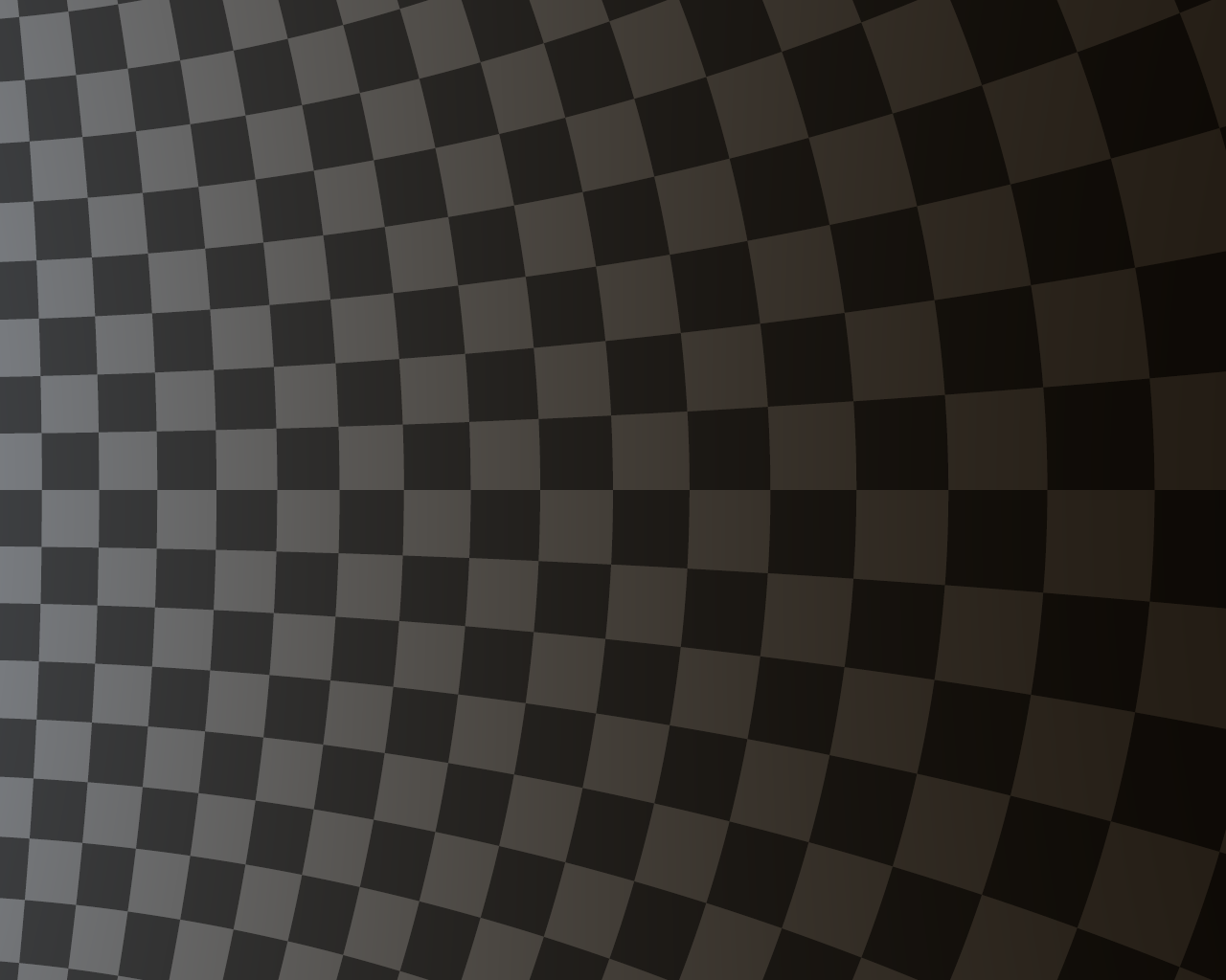
Figure 17: Same as Fig. 16 above, but now including color change due to Doppler shift. The bolometric intensity of each pixel of the celestial sphere is kept unchanged, so that the intensity changes that are seen are due to the variation of sensitivity of the eye with respect to the variable temperature, the loss of sensitivity being largest in the rear direction, where the red spectrum peaks in the infrared domain and has an intensity in the visible band that is exponentially suppressed as redshift increases.

B.1.3 Intensity

In addition to the frequency shift, the Doppler effect produces a variation of the overall intensity of a light source. In the case considered here, where we assume that our celestial sphere (and, later, the stars) have a black-body emission, the bolometric luminosity varies as $T^{4}$, where $T$ corresponds to the temperature of the celestial sphere pixel or star of interest. Consequently, the bolometric luminosity is modulated by a factor $(1+z)^{-4}$, where the redshift $z$ is given by

$$1+z=\frac{\omega}{\omega^{\prime}}.$$ (143)

The intensity variation therefore varies of a factor $[(1+v)/(1-v)]^{2}$ between the front and rear directions, a factor which can be quite large for relativistic velocities ($\sim 360$ for $v=0.9$), which make it difficult to represent on a computer screen since with sRBG coordinates, the relative intensity between the brightest pixel and the dimmest one (for a fixed hue) is $12.92\times 255=3294.6$. Note however that such a factor is valid for the bolometric luminosity only. Taking into account the eye response drastically change this factor, although it does not improve much the situation: a highly redshifted object become completely invisible not because its bolometric luminosity decreases, to the $(1+z)^{-4}$ factor but because almost all its energy becomes radiated in the infrared domain which is not visible at all to a human eye. An example of the intensity effect is shown in Fig. 18.

Figure 18: Same as Fig. 16 and 17 above, but now including everything. The luminosity gradient as one goes from the front to rear direction is even larger than previously since, in addition to that of the previous figure, it is modulated by an extra $(1+z)^{-4}$ factor, which here, for $v=0.5$, varies from $9$ in the front direction to $1/9$ in the rear one.

B.1.4 Amplification

When considering our checkerboard-like celestial sphere, the total intensity of a given square relies on the combination of its temperature change because of the Doppler effect and its angular size change because of aberration. This last part is computed implicitly by the fact that the number of pixels which span the square changes because of aberration. If we consider a star, then only the Doppler term is known a priori. However, the star is an extended object, although a tiny one, just as our checkerboard is. Therefore, we must add to its intensity change the amplification factor whose computation is outlined in Section V.2.

B.2 General relativistic effects only

B.2.1 Light bending

Let us now add a black hole to our scenery. An example of the same picture with and without the black hole is shown on Figure 19. The observer is looking toward latitude $-32.4\,{\rm deg}$ with respect to the coordinate grid we use. the visualization parameters are the same as previously.

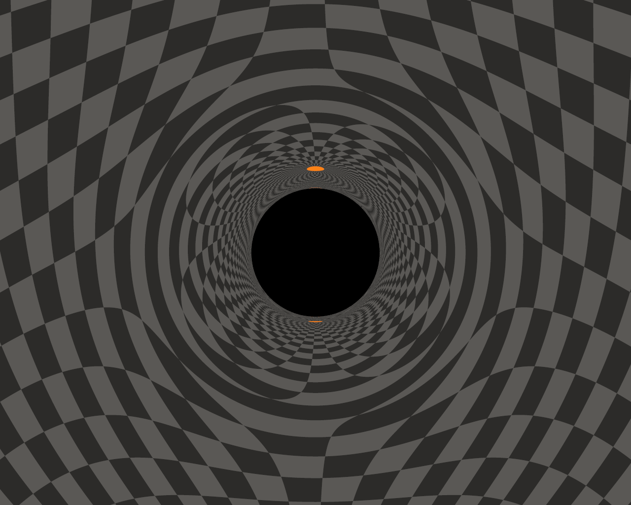
Figure 19: Comparison of a view seen by a static observer with and without the presence of the black hole. In the latter case, the observer lies at coordinate $r=30M$. The black hole lies in front of the most central dark square of the top picture. This square is seen highly distorted surrounding the silhouette of the black hole in the second picture. The two poles of the coordinate grid are seen as secondary/ghost images between the silhouette and the distorted black square, the south pole ghost image appearing above and that of the north pole below. Note that the second image is very slightly brighter than the first one because we have included the gravitational blueshift, which here takes the value $z=\sqrt{1-2M/r}-1\sim-0.0339$. However strange it may look like, such picture is nothing more than the visual translation of the deflection function shown in Fig. 1.

From a visual point of view, the central region of the picture, where we put the black hole, is now scattered all around (and at some distance) of the black hole silhouette. Therefore, the presence of the black hole somehow pushes away the background image as compared to the undistorted case. Between the distorted image of the celestial sphere lies a series of ghost images which we will discuss below.

B.2.2 Gravitational blueshift

For any geodesic, the quantity $E\equiv\dot{t}(1-2M/r)$ is conserved. If we denote by $\omega$ the $\dot{t}_{\gamma}$ component of some null geodesic, which means that the frequency of such photon measured by an observer at rest and at infinity will be $\omega$, then the $\dot{t}_{\gamma}$ component will be everywhere given by

$$\dot{t}_{\gamma}=\frac{\omega}{1-\frac{2M}{r}}.$$ (144)

Now, if we consider a static observer outside the black hole, the only component of his/her four-velocity will be $\dot{t}_{\rm obs}=(1-2M/r)^{-\frac{1}{2}}$. Therefore the frequency that such observer crossing a null geodesic coming from infinity will be

$$\omega^{\prime}=g_{tt}\dot{t}_{\gamma}\dot{t}_{\rm obs}=\omega\dot{t}_{\rm obs}=\omega\left(1-\frac{2M}{r}\right)^{-\frac{1}{2}}.$$ (145)

The corresponding blueshift that will be measured is therefore

$$z_{\rm grav}=-1+\frac{\omega}{\omega^{\prime}}=-1+\sqrt{1-\frac{2M}{r}}.$$ (146)

A few pictures on the increasing blueshift (and hence, the increasing brightness) as a static observer approaches to horizon is shown on Fig. 20

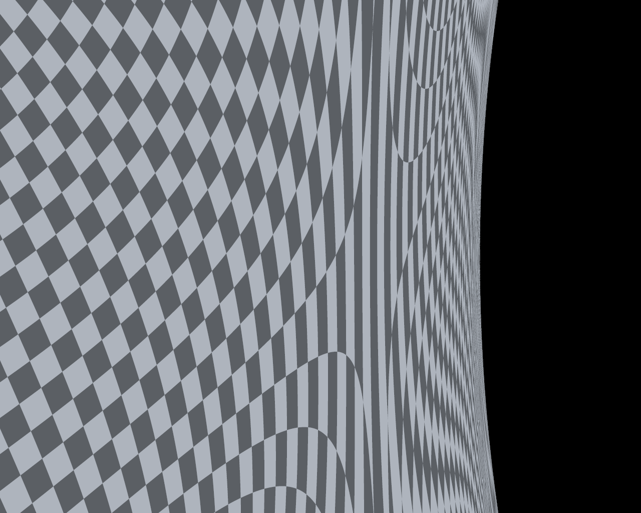
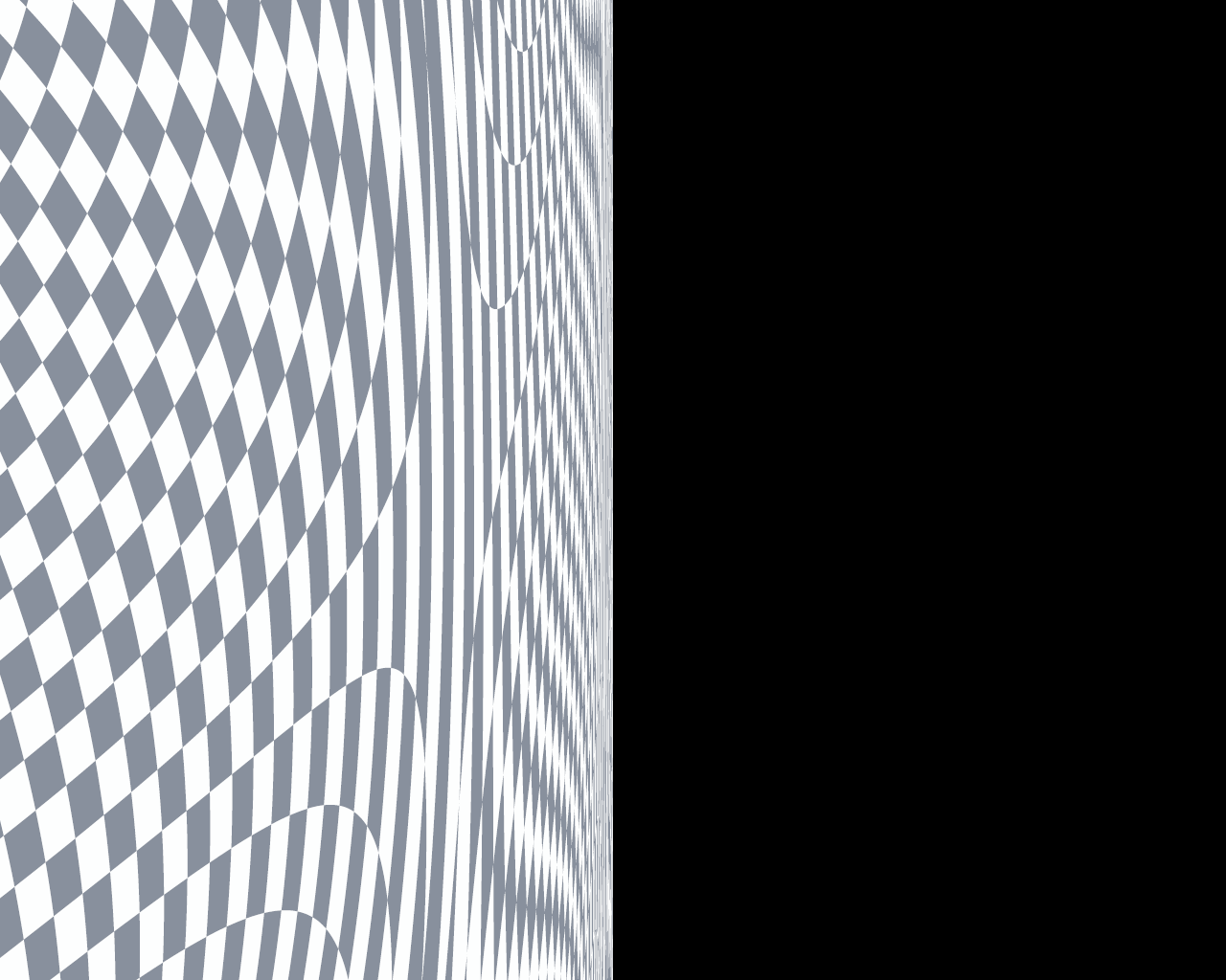
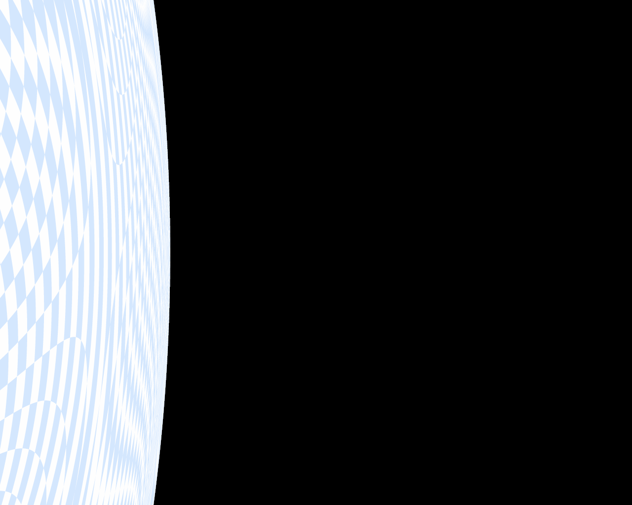
Figure 20: Three views of the vicinity of the black hole as seen by a static observer that stands at $r=4M$, $r=3M$, and $r=2.5M$ (from top to bottom). As is well-known, the $r=3M$ radial coordinate corresponds to that where photons can have (unstable) circular orbits around the black hole, so that in practice the black hole silhouette spreads over a half sphere for a static observer. Below this value of $r$, the silhouette no longer looks convex, but concave instead. The increasing brightness as $r$ decreases is due to the increasing blueshift $z_{\rm grav}$, which takes values $\simeq-0.293$, $\simeq-0.423$ and $\simeq-0.553$, respectively. Because of our choice of rendering, highly blueshifted stars would have smeared the view of last image, and have therefore been removed, and region I celestial sphere was replaced by a coordinate grid which makes more explicit the deformation at the edge of the black hole silhouette.

B.2.3 Lensing

As it is obvious from the distortion of central dark square of Fig. 19, the distortion of image induced by the black hole also modifies the angular size of background objects. This is the so-called gravitational lensing effect. In order to illustrate it, we reproduce the second image of Fig. 19 by modulating its intensity by the factor $f$ defined in Eq. (85). The result is shown in Fig. 21. As is well known, the point of the celestial sphere which happens to be exactly behind the black hole experiences an infinite amplification, at least a long as one considers geometric optics, and appears as an infinitely bright circle around the black hole, i.e., the so-called Einstein ring. The opposite point on the celestial sphere experiences the same behaviour and can be seen much closer to the black hole silhouette as shown in the accompanying Figure.

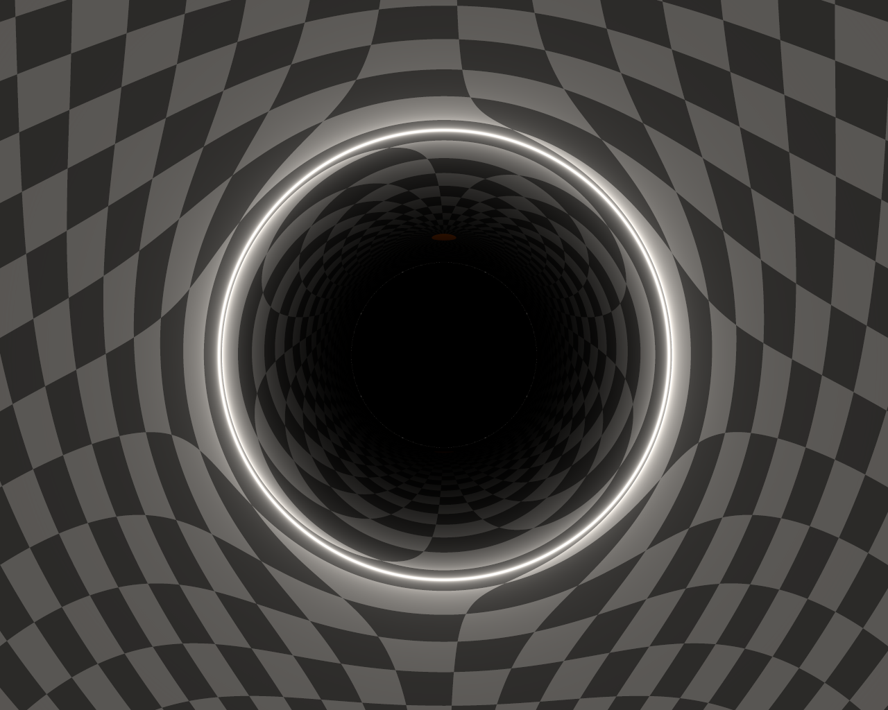
Figure 21: An illustration of the amplification and de-amplification phenomena induced by deflection of light. Standard calculation indicate that the region opposite to the black hole is slightly de-amplified, whereas amplification increases as one approaches the Einstein ring. Within the Einstein ring, amplification decreases drastically and de-amplification kicks in till one goes very close to the black hole silhouette (top picture). Then, a tiny region of amplification appears, which corresponds to the Einstein ring of the black hole anticenter. Because the width on the second amplification region is extremely small, one needs a fairly large zooming factor in order to see it (bottom picture, showing the upper left quadrant of the black hole silhouette).

B.2.4 Multiple images

A star that lies close to the direction that is exactly behind the black hole from the observer point of view will show two distinct images, corresponding to light rays that pass on each side of the black hole, while belonging to the plane containing the black hole, the observer and the star. These sets of double images can be easily spotted on any image, especially when the star direction is sufficiently close to the observer-black hole axis, so that each star image experiences lensing. However, even when this is no longer the case, double images can be spotted, although with more difficulty. It is to be noted that because geodesics in the Schwarzschild metric are planar, each star image lies on a great circle on which also lies the null radial geodesic going from the observer to the black hole. If one uses stereographic projection, these three points lies along a straight line along the screen if seen by a static observer. Figure 22 shows an example of multiple image in a simulated, visually realistic astronomical background.

Figure 22: A few examples of multiple images in an astronomically realistic simulated view. In the upper left quadrant, the circled pair of stars correspond to $\alpha$ and $\beta$ Centauri, and the single circled star is $\gamma$ Crucis. In the lower left quadrant, the the circled structure is the Small Magellanic cloud, the Large Magellanic cloud being the very large U-shaped structure above and below the black hole silhouette. The bright, circled star to in the right is $\alpha$ Carinae. Each pair of these stars are, for one outside the Einstein ring (large circle around the black hole silhouette), and for the other, inside. The only exception is for a star that is almost exactly behind the black hole, whose two image lie (almost) exactly on the Einstein ring. This is the case for the highly lensed, otherwise anonymous mag 7 star HD49359. The circled star inside the Einstein ring whose primary image is not seen is Sirius, whose primary image is off-screen (too much to the right), but whose secondary image is still easily visible despise de-amplification thanks to the very low magnitude of the unlensed star.

In some rare occasion, on can see more than two images of a given star. If the observer does not stand too close to the black hole, this occurs mostly for stars that lie along the observer-black hole axis, as it is the case for star HD49359 of Fig. 22. Zoomed-in versions of this view showing two extra ghost images of this star are shown in Fig. 23.

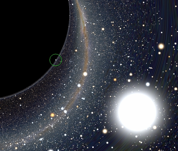
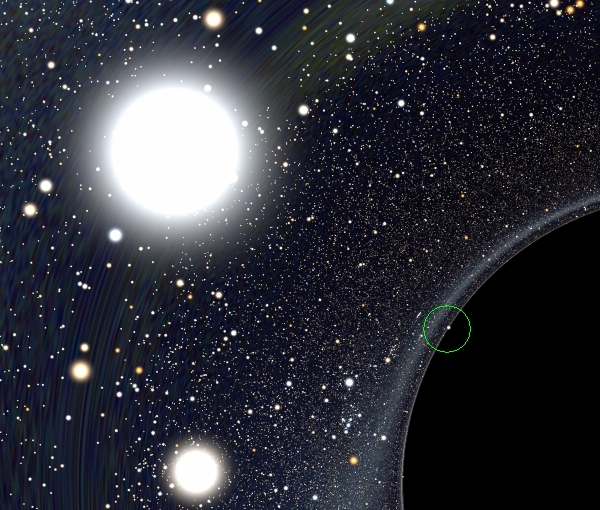
Figure 23: When zooming in between HD49359 primary or secondary image and the silhouette of the black hole, one sees two ghost images of this star, all of which lie within the segment joining the previous two images.

The amount of deflection a light ray experience when approaching the black hole increases indefinitely as its impact parameters approaches the critical value $3\sqrt{3}M$ (see Fig. 1). Consequently, there exists an infinite number of multiple images, all of which appear increasingly close to the edge of the lack hole silhouette. Such images can be seen only if one zooms in by a fairly large factor, as exemplified in Fig. 24.

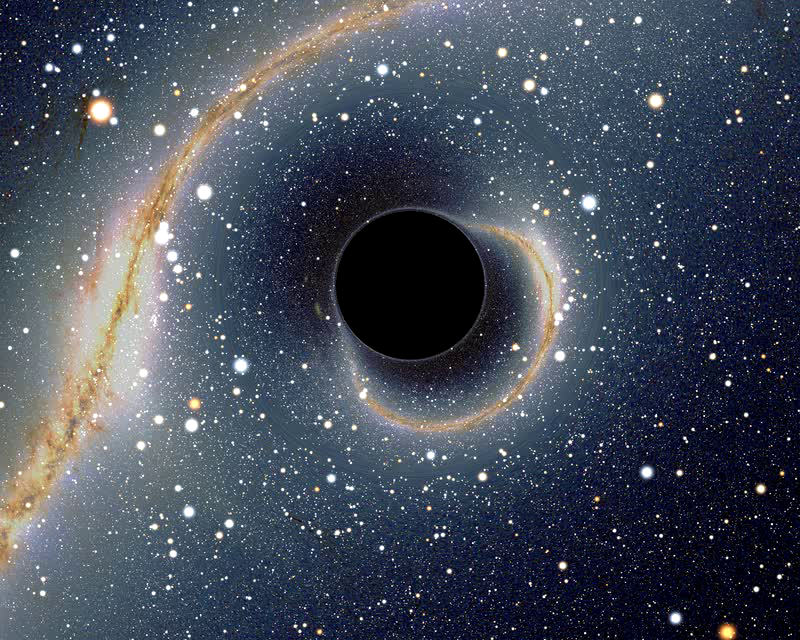
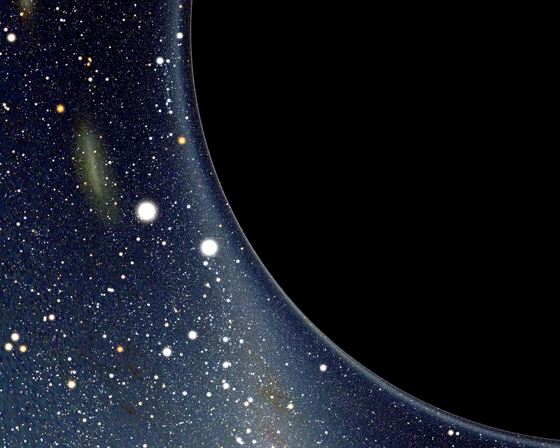
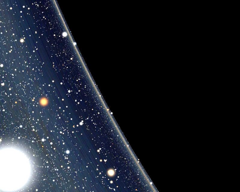
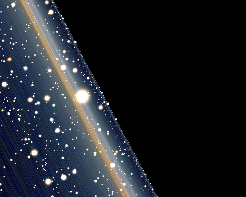
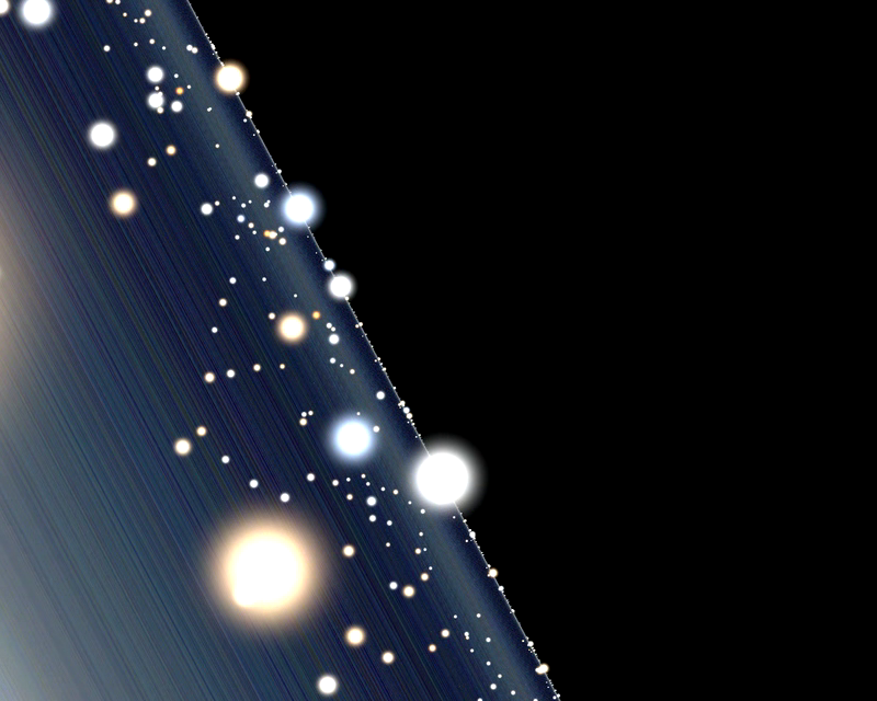
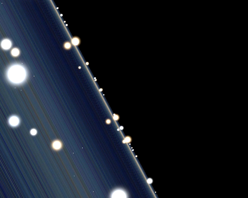
Figure 24: An example of the multiple image phenomenon in the Schwarzschild metric. One starts with an image with a 90 degrees field of view, and each subsequent view (from left to right, then top to bottom) has a zoom factor of around 4 with respect to the previous one, so that the last one has a field of view around $160\,{\rm mas}$. The first view shows the primary image of the Galactic disk, as well as its first “C”-shaped ghost image. The thin halo around the black hole corresponds to the second ghost image. The 2^nd view shows part of the first ghost image of the disk, as well as the ghost image of the Large Magellanic cloud. The second ghost image is now seen to be slightly away from the edge of the black hole silhouette (especially in the bottom part of the view). In the 3^rd view, one sees the first ghost image as a large band in the left of the image, and the second ghost image is now clearly visible. It is still visible in the 4^th view, which also shows the third ghost image. Note that each successive ghost image is alternatively bright then dim because they correspond to opposite parts of the Galactic disk, whose luminosity is not uniform. In the 5^th view, the third ghost image has been broadened on the left, whereas the fourth ghost image appears detached from the edge of the silhouette. This fourth image is now quite broadened on the 6^th view, which show the fifth ghost image of the disk, close to the edge of the silhouette. This fifth ghost image is then seen on the 7^th and 8^th views, together with the sixth ghost image, and, in the last view, the seventh ghost image. Note that the number of stars decreases as one zooms in, because of the finiteness of our star catalog. A deeper star catalog would be obviously necessary for the last views. Also, assuming that stars are pointlike sources may be questionable here since at that resolution stars angular size might possibly become visible, and make them appear as very elongated thin segments.

B.3 Combined effects

B.3.1 Circular orbits

One can combine special and general relativistic effects by considering an observer who is moving around a black hole. The simplest example corresponds to that of a circular orbit. As is well known, a timelike observer around a Schwarzschild black hole experiences a radial potential of the form

$$V(r)\propto\left(1-\frac{2M}{r}\right)\left(1+\frac{L^{2}}{r^{2}}\right),$$ (147)

where $L$ is the observer angular momentum per unit of mass. A stable circular orbit corresponds to the local minima of $V$, which correspond of the largest of the roots of equation

$$Mr^{2}-L^{2}r+3L^{3}M=0,$$ (148)

whose smallest value is $r=6M$. For a fixed orbit radius, the observer’s four-velocity $u_{\rm circ}^{\mu}$ is then given by its constants of motion, with

$$L^{2}=\frac{Mr}{1-\frac{3M}{r}},$$ (149)

and

$$E\equiv g_{tt}u_{\rm circ}^{t}=\frac{1-\frac{2M}{r}}{\sqrt{1-\frac{3M}{r}}},$$ (150)

so that one has, assuming that the orbital plane lies within the equatorial $\theta=\pi/2$ plane,

$$u_{\rm circ}^{t} = \frac{1}{\sqrt{1-\frac{3M}{r}}},$$ (151)

$$u_{\rm circ}^{\varphi} = \frac{Mr^{-\frac{3}{2}}}{\sqrt{1-\frac{3M}{r}}}.$$ (152)

The orbital velocity $v_{\rm circ}$ with respect to an observer situated at the same radial coordinate is then given by $u_{{\rm stat},\mu}u_{\rm circ}^{\mu}=\gamma=(1-v_{\rm circ}^{2})^{-\frac{1}{2}}$, where $u_{\rm stat}^{\mu}$ is the static observer four-velocity, whose only non zero component is $u_{\rm circ}^{t}=(1-2M/r)^{-\frac{1}{2}}$. The velocity is then

$$v_{\rm circ}=\sqrt{\frac{\frac{M}{r}}{1-\frac{2M}{r}}}.$$ (153)

Neglecting the denominator gives the well-known formula of the non relativistic third Kepler law. For orbital radii of $r=30M$ and $r=6M$, the orbital velocity is therefore $v_{\rm circ}\simeq 0.189c$ and $v_{\rm circ}=0.5c$, respectively. In order to determine the maximum redshift and blueshift an observer experiences, one has to combine the gravitational redshift formula (146) with the kinetic one (140), the combined redshift $z_{\rm tot}$ being given by

$$1+z_{\rm tot}=(1+z_{\rm grav})(1+z_{\rm kin}).$$ (154)

For an observer at $r=6M$, the maximum blueshift (in the front direction) is thus $z_{\rm max}=\sqrt{2}/3-1\simeq-0.529$, and the maximum redshift (in the rear direction) is $z_{\rm min}=\sqrt{2}-1\simeq 0.414$. Fig. 25 shows a comparison between the side view seen by a $r=30M$ observer looking toward the black hole, and the front view seen by a $r=6M$ observer, both in circular orbit.

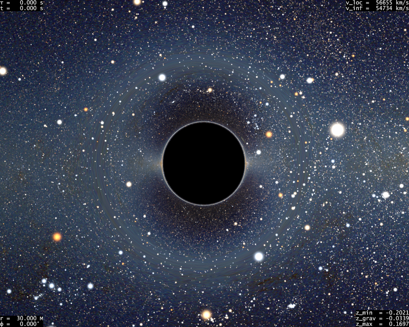
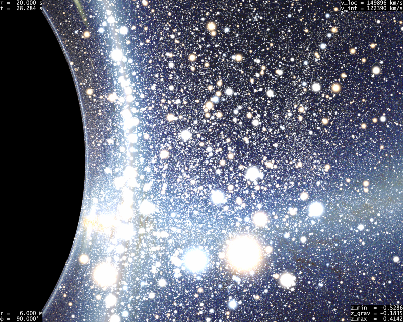
Figure 25: Comparison of two circular orbits, with radii $r=30M$ (top) and $r=6M$ (bottom). In the first trajectory, the velocity is weakly relativistic, so that special relativistic effects are moderate. The direction of motion, which is on the right of the image, is only thus only moderately brighter than the opposite one. On the contrary, there is a very strong brightening in the second image, since the observer is now subject to a large kinetic blueshift (since orbital velocity is half of the speed of light here) and a significant gravitational blueshift (since the observer is close to the black hole). Similarly, the star background is fairly recognizable in the first picture. One can for example spot a somewhat flattened version of Orion constellation in the lower left quadrant of the image as well as a flattened Taurus in the bottom centre. This is no longer the case in the second one, where even familiar constellations are difficult to spot because the star background is now so crowded. Large blueshift allows some highly blueshifted cold stars to overcome the usually brighter stars we are used to see. There are, for example, many more bright, orange, stars (i.e., usually cold and faint stars) around Ursa Major constellation in the upper right quadrant of the image.

B.3.2 Non circular, non radial trajectories

Let us switch to geodesic non circular trajectories. Relativistic equivalent of Newtonian parabolic trajectories correspond to trajectories with zero velocity at infinity but non zero angular momentum $L$ per unit of mass. Simple algebra then show that periastron radial coordinate is given by

$$\frac{r_{\rm per}}{M}=\frac{1}{\frac{1}{4}-\sqrt{\frac{1}{16}-\frac{M^{2}}{L^{2}}}},$$ (155)

and velocity at periastron is

$$v_{\rm per}=\sqrt{\frac{2M}{r}}.$$ (156)

Obviously, such a relativistic equivalent of a parabolic trajectory has a periastron bounded by $r=4M$, and the maximal velocity at periastron is then $v=c/\sqrt{2}$. Now, the trajectory in itself turns much more around the black hole than a parabola because of the extreme relativistic shift of periastron it experiences (the so-called zoom-and-whirl effect), and the azimuthal angle shift between far from the black hole and periastron is much bigger than $\pi/2$. Fig. 26 gives an example of an almost extremal pseudo-parabolic trajectory.

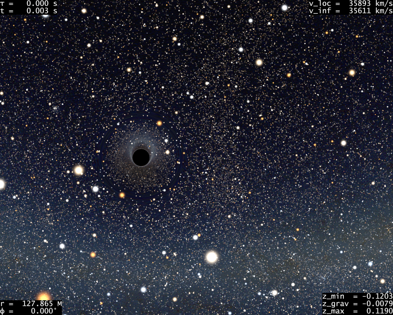
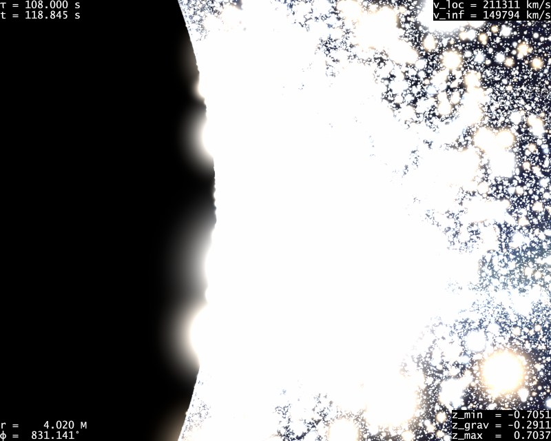
Figure 26: Two views of an almost extremal pseudo parabolic orbit, starting from infinity a zero velocity and angular momentum close to the minimum allowed value of $4M$ (see Eq. (155)). Top image corresponds to a view far from the black hole, where the trajectory is close to radial. Bottom image corresponds to a view earlier than, but very close to periastron, at $r=4.02M$. Local velocity, given by Eq. (156) is very close to $c/\sqrt{2}$, and velocity measured by a distant observer, given by $v_{\rm inf}=v_{\rm per}\sqrt{1-2M/r}$ is very close to $c/2$. Note that the azimuthal angle shift between the two view is $\sim 831$ deg., much larger than the Newtonian analog which should be slightly smaller than $180$ degrees.

One can also have trajectories which are the relativistic equivalent of Newtonian hyperbolic trajectories. In this case, a convenient set of parameters describing the trajectory are the velocity at infinity and the impact parameter. Conversely, one can determine which is the minimum velocity at infinity, $v_{\infty}$, that allows to reach a given value of the radial $r_{\rm per}$ coordinate at periastron. After some algebra, it appears that this is conveniently done if we parametrize the periastron radial coordinate by the quantity $e$, $1<e<3$, such that

$$r_{\rm per}=\frac{2(3+e)}{1+e}M,$$ (157)

then the velocity at infinity must be greater than

$$v_{\infty}>\sqrt{\frac{e^{2}-1}{8}}.$$ (158)

Equivalently, this minimum velocity can be expressed as a function of $r_{\rm per}/M$ :

$$v_{\infty}>\frac{\sqrt{4-\frac{r_{\rm per}}{M}}}{\frac{r_{\rm per}}{M}-2}.$$ (159)

Figures 27 and 28 show two example of such near extremal pseudo-hyperbolic trajectories.

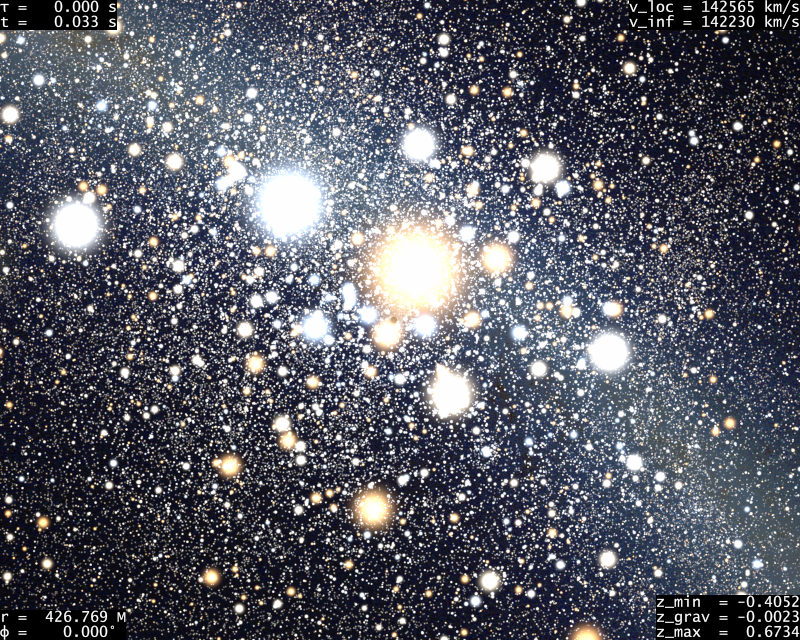
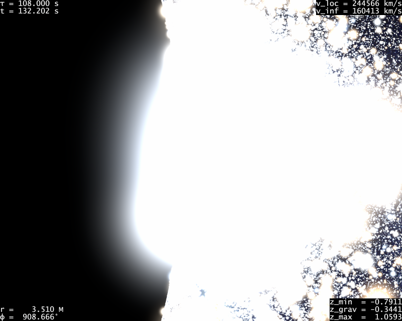
Figure 27: Pseudo hyperbolic trajectory with a periastron radial coordinate of $3.5M$, which necessitates a velocity at infinity at least larger than $\sqrt{2}c/3\sim 141323\,{\rm km}/{\rm s}$ (actual value chosen here is very slightly higher). A velocity close to that value is reached far from the black hole in the top view. Bottom view is computed close to periastron. The black hole mass is the same here as in the previous Figure, and the proper time interval between first and second view is also the same. Consequently, since bottom view in both figures are close to periastron, top view radial coordinate is large in this Figure than in the previous one because velocity far from the black hole is larger. Black hole angular size is in addition further reduced by the stronger aberration of this Figure, so that it is barely visible (below the brightest central, orange star). Note also that the background sky is much brighter, as expected.

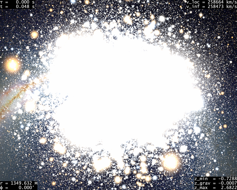
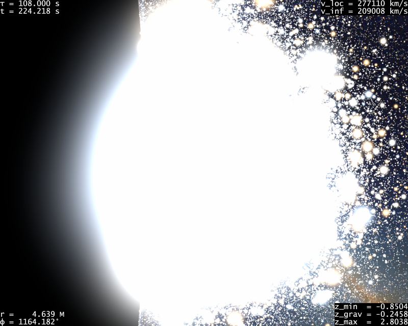
Figure 28: Same as Fig. 27, except that periastron now occurs at $r=3.1M$, which necessitates an initial velocity greater than $v\sim 0.862c\sim 258552\,{\rm km}/{\rm s}$. On the top picture, the black hole angular size is so small and the star background so bright that the black hole silhouette is invisible with our rendering choices.

References

- (1) S. Chandrasekhar, The Mathematical Theory of Black Holes, Oxford University Press, England (1983).
- (2) J. M. Bardeen, In “Houches Lectures: 1972, Black Holes”, C. Dewitt ed., pp. 215-239.
- (3) J.-P. Luminet, Astronomy and Astrophysics, 75, 228-235 (1979).
- (4) J. Fukue & T. Yokoyama, Publ. Astr. Soc. Jap., 40, 15–24 (1988).
- (5) S. U. Viergutz, Astron. Astrophys., 272, 355 (1993).
- (6) J.-A. Marck, Class. Quant. Grav., 13, 393-402 (1996).
- (7) C. Fanton et al., Publ. Astr. Soc. Jap., 49, 159–169 (1997).
- (8) H. Falcke, F. Melia & E. Agol, ApJ q Letters, 528, L13–L16 (2000).
- (9) A. J. S. Hamilton, Bulletin of the American Astronomical Society, 36, 810 (2004); See also dedicated website http://jila.colorado.edu/~ajsh/insidebh/intro.html.
- (10) K. Beckwith & C. Done, Month. Not. Roy. Astr. Soc., 359, 1217–1228 (2005).
- (11) S. Gillessen et al., Astrophysical Journal, 692, 1075–1109 (2009).
-
(12)
European Southern Observatory and Max Planck
Institue for Extraterrestrial Physics GRAVITY webpages:
https://www.eso.org/sci/facilities/develop/instruments/gravity.html, http://www.mpe.mpg.de/ir/gravity. - (13) Event Horizon Telescope website: http://www.eventhorizontelescope.org/.
- (14) F. H. Vincent et al., Class. Quant. Grav., 28, 225011 (2011).
- (15) A. E. Broderick et al., ApJ, 735, 110 (2011).
- (16) C. Chan, D. Psaltis & F. Özel, ApJ, 777, 13 (2013).
- (17) A. E. Broderick et al., ApJ, 784, 7 (2014).
- (18) T. Muller & D. Weisskopf, Am. J. Phys., 78, 204 (2010).
- (19) O. James et al., Class. Quant. Grav., 32, 065001 (2015).
- (20) G. Gamow, Mr Tompkins in Wonderland, Cambridge University Press, Cambridge, England (1940).
- (21) J. Úbeda, S. Marquès & E. Pons, The Dalídimension (DVD), Music Video Dist. (2008), ASIN: B001BWYT4E.
- (22) H.-P. Nollert & H. Ruder, Was Einstein gerne gesehen hätte, Spektrum Der Wissenschaft, Lörrach, BW, Germany (2005).
- (23) C. M. Savage, A. C. Searle & L. McCalman, arXiv:physics/0607223; C. M. Savage, A. C. Searle & L. McCalman, American Journal of Physics, 75, 791-798 (2007); See also dedicated website at http://www.anu.edu.au/physics/Searle/ .
- (24) A. J. S. Hamilton & G. Polhemus, New Journal of Physics, 12, 123027 (2010).
- (25) É. Gourgoulhon, Relativité Restreinte, EDP Sciences, Les Ulis, France (2010).
- (26) K. S. Thorne, R. H. Price, D. A. MacDonald, Black Holes: the Membrane Paradigm, Yale University Press, New Haven (1986).
- (27) S. M. Carroll, Lecture Notes on General Relativity, arXiv:gr-qc/9712019.
- (28) W. H. Press et al., Numerical Recipes in C, 2ndedition, Cambridge University Press, Cambridge, Great Britain (1992).
- (29) M. D. Kruskal, Phys. Rev., 119, 1743–1745 (1960).
- (30) S. W. Hawking & G. F. R. Ellis, The large scale structure of space-time, Cambridge University Press, Cambridge, Great Britain (1973).
- (31) R. M. Wald, General Relativity, The University of Chicago Press, Chicago, United States (1984).
- (32) K. Giampedakis & D. Kenneflick, Phys. Rev. D, 66, 044002 (2002).
- (33) S. Seitz, P. Schneider & J. Ehlers, Class. Quantum Grav., 11, 2345-2373 (1994).
- (34) Commission internationale de l’Éclairage proceedings, Cambridge University Press, Cambridge (1931). Appropriate material can also be found in many modern monographies such as R. W. Hunt, Measuring colour (3rded.), Fountain Press, England (1998).
- (35) See, e.g., S. Brunier & A. Fuji, The Concise Atlas of the Stars, Firefly Books (2005). Some less spectacular but online pictures can be found on various locations such as the Hubble Space Telescope website, http://www.spacetelescope.org/images/?search=akira+fuji .
- (36) A. Mellinger, Publications of the Astronomical Society of the Pacific, 121, 1180-1187 (2009). See also website http://home.arcor-online.de/axel.mellinger/ .
- (37) S. Brunier, http://sergebrunier.com/gallerie/pleinciel/ .
- (38) E. Bertin, & S. Arnouts, Astronomy & Astrophysics Supplement, 317, 393–404 (1996).
- (39) The 2MASS infrared sky, part of the 2MASS outreach website, http://www.ipac.caltech.edu/2mass/gallery/showcase/allsky/index.html .
- (40) L. M. Bugayevskiy & J. P. Snyder, Map projections, A reference Manual, Taylor & Francis, London (1995).
- (41) ftp://cdsarc.u-strasbg.fr/pub/cats/III/135A/ .
- (42) N. V. Karchenko, Kinematika i Fizika Nebesnykh Tel, 17, 409–423 (2001); electronic version available at URL http://cdsarc.u-strasbg.fr/viz-bin/Cat?I/280B .