Automatic Region-wise Spatially Varying Coefficient Regression Model: an Application to National Cardiovascular Disease Mortality and Air Pollution Association Study

Abstract

Motivated by analyzing a national data base of annual air pollution and cardiovascular disease mortality rate for 3100 counties in the U.S. (areal data), we develop a novel statistical framework to automatically detect spatially varying region-wise associations between air pollution exposures and health outcomes. The automatic region-wise spatially varying coefficient model consists three parts: we first compute the similarity matrix between the exposure-health outcome associations of all spatial units, then segment the whole map into a set of disjoint regions based on the adjacency matrix with constraints that all spatial units within a region are contiguous and have similar association, and lastly estimate the region specific associations between exposure and health outcome. We implement the framework by using regression and spectral graph techniques. We develop goodness of fit criteria for model assessment and model selection. The simulation study confirms the satisfactory performance of our model. We further employ our method to investigate the association between airborne particulate matter smaller than 2.5 microns (PM 2.5) and cardiovascular disease mortality. The results successfully identify regions with distinct associations between the mortality rate and PM 2.5 that may provide insightful guidance for environmental health research.

Keywords: air pollution, areal data, environmental health, segmentation, spatial statistics, spatially varying associations.

1 Introduction

The recent environmental health research has revealed that the associations between air pollution exposures and health outcomes vary spatially because the local environmental factors including topography, climate, and air pollutant constituents are heterogeneous across a broad area (Bell et al.,, 2014; Chung et al.,, 2015; Garcia et al.,, 2015). However, the current available region definition (e.g. the 48 states of the continental U.S.) can not ensure homogeneous intra-region exposure-health-outcome association (EHA). Therefore, it is desirable to identify a set of disjoint regions exhibiting similar within-region EHAs and distinct between-region EHAs in a data-driven fashion (automatic rather than predefined region map). The statistical inferences based on the automatic detected regions (e.g. EHA regression analysis) can provide important guidance for environmental health research.

Motivated by analyzing a data set from the national data base of annual air pollution exposures and cardiovascular disease mortality rates for 3100 counties in the U.S. during the 2000s (more details are provided in section 4), we aim to estimate the spatially varying associations between air pollution exposures and health outcomes across different regions. The region level inferences may reveal local environmental changes and latent confounders that could influence local population health. However, most current spatial statistical models (for areal data analysis) are limited for this purpose because few of them allow data-driven allocation of counties into contiguous regions (that different regions demonstrate distinct health risks). In our analysis, we use county as the basic spatial unit because the health outcome data is aggregated at the county level, yet the proposed approach could be applied for analysis with any basic spatial unit (e.g. zip code).

The most popular modeling strategy for areal spatial data has been through the conditionally autoregressive (CAR) distribution and its variants.(Besag,, 1974; Besag et al.,, 1991; Gelfand and Vounatsou,, 2003; Banerjee et al.,, 2004; Waller and Gotway,, 2004; Cressie and Wikle,, 2011). In disease mapping, a random effect model is often employed to link the disease rate with exposures, and the random residuals and random slopes are used to account for spatial dependence via CAR or multivariate CAR (MCAR) priors (Gelfand et al.,, 2003; Waller et al.,, 2007; Wheeler et al.,, 2008; Banerjee et al.,, 2008). Although the random residuals and slopes could improve goodness-of-fit by explaining more proportion of variance, the inferences on the regression coefficients (main effects) are still limited to one value for the whole nation(Waller and Gotway,, 2004). The spatial dependency information is incorporated into statistical modeling by using a spatial adjacency matrix $W$ where $W_{ij}=1$ if $i$ and $j$ are adjacent neighbors and otherwise $W_{ij}=0$. It has been recognized that the spatial adjacency may not necessarily lead to similar random effects because health outcomes related factors such as landscape types (e.g. urban area and forest) or sociodemographic factors (e.g. income levels) could be distinct between neighbors. Lu and Carlin,, 2005 propose a Bayesian hierarchical modeling framework to detect county boundaries by using boundary likelihood value (BLV) based on the posterior distributions, yet the detected boundary segments are often disconnected (Ma and Carlin,, 2007). $L_{1}$ norm CAR prior has also been applied to account for abrupt changes between neighbors (Best et al.,, 1999; Hodges,, 2003). Ma and Carlin,, 2010 further include the random effect for the boundary edges with Ising priors and identify more connected boundary segments. Although the boundaries can provide information of adjacent but distinct neighbors, they may not allow to define distinct regions due to the discontinuity of boundary edges. It is also worth to note that the boundaries are often defined based on the outcomes (or residuals) rather than the disease-exposure associations (regression coefficients).

To fill this gap, we present an automatic region-wise spatially varying coefficient method to recognize and estimate the spatially varying associations between air pollution exposures and health outcomes in automatically detected regions for environmental health data, and we name it as region-wise automatic regression (RAR) model. Rather than focusing on modeling the spatial random effects, the RAR model aims to parcellate the whole spatial space into a set of disjoint regions with distinct associations, and then to estimate the association for each disjoint region. We implement the RAR model in three steps: first, we assess the initial difference of associations by examining each spatial unit’s impact on the overall regression coefficient based on $dfbeta$; second, based on the initial difference of the associations, we cluster the all spatial units into a set of spatially contiguous regions by using image segmentation technique; last, we estimate the associations for each region, and we account for the within region spatial correlation of the residuals. We also develop a likelihood based optimization strategy for parameter selection. Our main contribution is first to provide a statistical model to identify the data-driven definition of regions exhibiting differential regression coefficients that may yield significant public health impact.

The rest of this paper is organized as follows. In Section 2, we describe RAR model and its three step estimation procedure. In Section 3, we conduct simulation studies with the known truth to examine the performance of the RAR model and to compare it with existing methods. In section 4, we apply the proposed method to a environmental health dataset on investigating the association between PM 2.5 and cardiovascular disease mortality rate in the U.S.. We conclude the paper with discussions in section 5.

2 Methods

We use a graph model $G=\{V,E\}$ to denote the spatial data, where the vertex set $V$ represents all spatial units (e.g. counties) in the space/map and the edge set $E$ delineates the similarity between the vertices. For RAR model, $e_{ij}\in E$ reflects the similarity between the EHA of spatial units $i$ and $j$ ($i,j\in V$ and $|V|=S$).

In the following subsections, we introduce the three steps of RAR model: 1) to assess the spatial association affinity between spatial units ($e_{ij}$); 2) to parcellate graph $G$ into $K$ regions that $G=\cup_{k=1}^{K}G_{k}$ and $G_{k}\cap G_{k^{\prime}}=\emptyset$, and the spatial units within one region $G_{k}$ exhibit coherent coefficients; and 3) to estimate the region-specific EHA. For notational simplicity, we only consider cross-sectional study modeling though it is straightforward to extend the RAR method to longitudinal studies.

2.1 Step 1: The adjacency matrix $E=\{e_{ij}\}$

To assess the association between health outcomes and covariates, a Poisson regression model is often used:

$$Y_{i}|\mu_{i} \sim\mbox{Poisson}(\mu_{i}n_{i}),\mbox{ for all }i=1,\cdots,S$$

$$log(\mu_{i}) =\beta\mbox{PM2.5}_{i}+\boldsymbol{\eta}\textbf{X}_{i}$$ (2.1)

where $Y_{i}$ is death count and $n_{i}$ is age-adjusted expected population count for county $i$, and $\textbf{X}_{i}$ are covariates of potential confounders besides the air pollution exposure. If the association between air pollution exposure and health outcome at the location $i$ deviates from the general trend, then the regression coefficient excluding location $i$ $\boldsymbol{\beta}_{(i)}$ will be distinct from the general regression coefficient of all observations $\boldsymbol{\beta}$. Therefore, we adopt DFBETAs to measure the EHA deviation for location $i$. We denote $d_{i}$ as the deviation of spatial unit $i$:

$$d_{i}=\hat{\beta}_{(i)}-\hat{\beta}\approx\mbox{DFBETA}_{i}=\{(Z^{T}\Omega Z)^{-1}Z_{i}\Omega_{i}(1-h_{i})^{-\frac{1}{2}}r_{pi}\}_{PM2.5}/\hat{\sigma}(\hat{\beta})$$ (2.2)

where Z is the design matrix including both PM2.5 and $X$, $\Omega$ is weight matrix ( $\Omega$ is the identity matrix if no weight is assigned), $h_{i}$ is the leverage, $r_{pi}$ is the standardized Pearson residual, $\hat{\sigma}(\beta)$ is the estimated standard deviation of $\beta$ (Williams,, 1987). Note that 2.2 is a one-step approximation to the difference for a generalized linear model (Preisser and Qaqish,, 1996).

Then, the similarity of the associations between two spatially adjacent units $i$ and $j$ are calculated by a distance metric (e.g. Gaussian similarity function):

$$e_{ij}=\mbox{exp}(-\frac{(d_{i}-d_{j})^{2}}{2\widehat{\sigma_{d}}^{2}})\times\mbox{I}(i\sim j)$$ (2.3)

where $\widehat{\sigma_{d}}$ is the standard deviation across all $d_{i}$, and $\mbox{I}(i\sim j)$ is the indicator function which equals 1 only when $i$ and $j$ are spatially adjacent. In addition, if the natural cubic splines are used to fit the nonlinear trend of the air pollution exposure (Dominici et al.,, 2002), then $e_{ij}=exp(-\frac{1}{2}(\textbf{d}_{i}-\textbf{d}_{j})^{T}\widehat{\Sigma}^{-1}(\textbf{d}_{i}-\textbf{d}_{j}))$. Thus, the range of $e_{ij}$ is from 0 to 1. The similarity matrix $E$ is a $S\times S$ matrix, which is equal to $E^{0}\circ W$ ($E^{0}=\{\mbox{exp}(-\frac{(d_{i}-d_{j})^{2}}{2\widehat{\sigma_{d}}^{2}})\}$ and $\circ$ is Hadamard product ). Thus, matrix $E$ fuses information of PM2.5 exposure (along with other covariates) and health outcomes in $E^{0}$ with spatial adjacency information $W$.

2.2 Step 2: Spectral graph theory based automatic region detection

The goal of step two is to identify the disjoint and contiguous regions ($G=\cup_{k=1}^{K}G_{k}$) such that the EHA of the spatial units are homogeneous within each $G_{k}$ but distinct between $G_{k}$ and $G_{k^{\prime}}$ ($k\neq k^{\prime}$). The contiguity requires that $\forall i$ vertex in $G_{k}$, there exists at least one vertex $j$ which is connected to $i$. Then the region detection becomes a graph segmentation problem based on the similarity matrix $E$. We aim to estimate a set of binary segmentation binary parameters $\Delta=\{\delta_{ij}\}$ and $\delta_{ij}=0\mbox{ or }1$ that parcellate $G$ into $\{G_{k}\}$. Therefore, the segmentation model aims to estimate the latent binary parameters: $\widehat{\delta}_{ij}|e_{ij},N(e_{ij})$ with the contiguity constraint, where $N(e_{ij})$ is the neighborhood of edge $e_{ij}$. One way to circumvent this is to identify the $\widehat{\delta}_{ij}=0$ for those $e_{ij}>0$ in $E$ (which is analogous to “cutting” edges in the graph) with the optimization that:

$$\sum_{k=1}^{K}\frac{\mbox{cut}(G_{k},\overline{G_{k}})}{\mbox{vol}(G_{k})}$$

$$\mbox{cut}(G_{k},\overline{G_{k}})=\sum_{i\in G_{k},j\in\overline{G}_{k}}e_{ij}$$ (2.4)

where $K$ is the number of disjoint sets and $\mbox{cut}(G_{k},\overline{G}_{k})$ is the sum of a set of edge weights (with $e_{ij}>0$ and $\widehat{\delta}_{ij}=0$) to isolate the subgraph $G_{k}$ from $G$. However, even for a planary graph G and $K=2$ parcellation, the optimization is NP complex. To solve the objective function in 2.4, a two step relaxation procedure is often used. The first step is a continuous relaxation:

$$\mbox{minimize }\sum_{l=1}^{K}f^{\prime}_{l}Lf_{l}=\frac{1}{2}\sum_{l=1}^{K}\sum_{i\neq j}e_{ij}\|\frac{f_{l}(i)}{D^{1/2}_{e(i,i)}}-\frac{f_{l}(j)}{D^{1/2}_{e(j,j)}}\|^{2}$$

$$L=I-D_{E}^{-1}E$$ (2.5)

where L is the normalized graph Laplacian matrix with $D_{E}=Diag(e_{i+})$ ($e_{i+}=\sum_{j}e_{ij}$), and $f=\{f_{1},\cdots f_{K}\}$ is a $N\times K$ coordinate matrix (all entries are continuous) that places the close nodes (based on the adjacency matrix $E$) near to each other in $\mathbb{R}^{K}$, and $f_{l}$ ($l=1\cdots K$, $N\times 1$) is the $l$th vector (Chung,, 1997). By Rayleigh quotient, $f$ are the first $K$ eigen-vectors of spectral decomposition of $L$ (with ascending order of eigen-values) (Von Luxburg,, 2007). In addition, the unnormalized graph Laplacian matrix $L=D_{E}-E$ is also often used (Von Luxburg,, 2007). From the spectral graph theory point of view, the Bayesian CAR model updates the random effect ($\boldsymbol{\phi}$) posterior sampling by using the heuristic to increase the fusion of likelihood and the objective function in 2.5 which is equivalent to minimizing unnormalized graph Laplacian matrix ($L=D_{E}-E$). Therefore, the CAR prior can be considered as a penalty (restriction) term that aligns with the spectral clustering objective function.

The second step of the automatic region detection procedure is discretization relaxation that produces $f^{d}$ which is a $N\times K$ binary matrix with all entries either 0 or 1 and $f^{d}\textbf{1}_{K\times 1}=\textbf{1}_{N\times 1}$. Then, objective function becomes

$$\mbox{minimize }\sum_{l=1}^{K}f^{d^{\prime}}_{l}Lf^{d}_{l}=\frac{1}{2}\sum_{l=1}^{K}\sum_{i\neq j}e_{ij}\|\frac{f^{d}_{l}(i)}{D^{1/2}_{e(i,i)}}-\frac{f^{d}_{l}(j)}{D^{1/2}_{e(j,j)}}\|^{2},$$ (2.6)

which is equivalent to 2.4. The second step optimization aims to calibrates the $f^{d}$ coordinate matrix with reference to $f$. To implement this optimization step, Ng et al.,, 2002 and Shi et al.,, 2000 apply K-means clustering algorithms for the distretization relaxation. However, the K-means clustering algorithm results may vary due to different random initialization and yield unstable results. Yu and Shi,, 2003 develop multiclass spectral clustering algorithm which is robust to random initialization and nearly global-optimal. The optimization yields results of the automatic region detection, and based on $f^{d}$ all spatial units are categorized to $K$ class with contiguity. In addition, $\widehat{\delta_{ij}}$ can be obtained from the resulting $f^{d}$, and under mild regularity condition the spectral clustering based region segmentation estimator is consistent that is $\widehat{\delta_{ij}}\rightarrow\delta_{ij}$ (Von Luxburg et al.,, 2008, Lei and Rinaldo,, 2014). We briefly summarize the algorithm in Appendix and refer the readers to the original paper for the detailed optimization algorithm.

As a comparison, the popular Bayesian CAR model leverages the second line of formula 2.1

$$log(\mu_{i})=\beta\mbox{PM2.5}_{i}+\boldsymbol{\eta}\textbf{X}_{i}+\phi_{i},$$

and imposes areal random intercept $\boldsymbol{\phi}=(\phi_{1},...,\phi_{S})$ linked with the spatial adjacency matrix $W$ by letting $\boldsymbol{\phi}\propto exp(-\frac{\tau_{\phi}}{2}\boldsymbol{\phi}^{\prime}(D-\rho W)\boldsymbol{\phi})$. $\tau_{\phi}$ is a positive scale parameter, $W$ is the spatial adjacency matrix introduced in section 1, $D=Diag(w_{i+})$ ($w_{i+}=\sum_{j}w_{ij}$), and $\rho$ is chosen to ensure $(D-\rho W)$ non-singular. Note that the distribution of $\phi$ is a proper CAR distribution when $\rho\neq 0$.

When implementing the MCMC for a Bayesian CAR model, the chain updating criteria incorporate both the likelihood part $lik(y|\boldsymbol{\theta})$ and the CAR prior $exp(-\frac{\tau_{\phi}}{2}\boldsymbol{\phi}^{\prime}(D-\rho W)\boldsymbol{\phi})$. The parameter update rule in part favors smaller $\frac{\tau_{\phi}}{2}\boldsymbol{\phi}^{\prime}(D-\rho W)\boldsymbol{\phi}$ values, i.e. the spatially adjacent $\phi_{i}$ and $\phi_{j}$ have similar values. Interestingly, the prior function is intrinsically linked with the objective function of spectral clustering algorithm which aims to minimize $tr(\boldsymbol{f^{d}}^{\prime}(D-\rho W)\boldsymbol{f^{d}})=\sum_{l=1}^{K}\boldsymbol{f^{d}}_{l}^{\prime}(D-\rho W)\boldsymbol{f^{d}}_{l}$, where $D-\rho W$ is unnormalized graph Laplacian matrix when $\rho=1$ and $\boldsymbol{f^{d}}$ is discretized $N\times K$ (N nodes and K classes) matrix to represent the cluster membership that $\boldsymbol{f^{d}}\in\{0,1\}$ and $\boldsymbol{f^{d}}\boldsymbol{1}_{K}=\boldsymbol{1}_{N}$(Von Luxburg,, 2007). Using our similarity matrix $E$ as $W$, $tr(\boldsymbol{f^{d}}^{\prime}(D-\rho W)\boldsymbol{f^{d}})$ is smaller when the spatially adjacent units with similar DFBETAS are classified into one spatial cluster. With similar objective functions, $\boldsymbol{f^{d}}$ could be obtained by discretizing $\boldsymbol{\phi}$ (Von Luxburg,, 2007). Hence, both the CAR and RAR model incorporate spatial adjacency in a close format of the updating criteria and objective function. Yet, as the random effects (residuals or the random slopes) $\boldsymbol{\phi}$ in the CAR model are continuous, they could not provide region parcellation information to identify regions with distinct EHA as the RAR model does.

2.3 Step 3: Association estimation on the automatically detected regions

Provided with the automatic region parcellation results $G=\cup_{k=1}^{K}G_{k}$, we estimate the region/subgraph specific association between air-pollution exposure and health outcomes. The straightforward method is to conduct stratified analysis such that within each $G_{k}$, the GLM is estimated:

$$y_{i} \sim\mbox{Poisson}(\mu_{i}),\ \ \forall i\in G_{k}$$

$$g(\mu_{i}) =\beta^{k}\mbox{PM}_{i}+\boldsymbol{\eta}^{k}\textbf{X}_{i}.$$ (2.7)

Within each $G_{k}$, we further investigate the spatial dependence of the residuals by using semivariogram or Moran’s I statistic. If the residuals of the spatially close units are dependent with each other, then the spatial autoregressive models such as CAR and SAR can be applied for regression analysis. Alternatively, a GLM could be applied to fit all spatial units by using the region indicator as a categorical covariate and adding the interaction terms of the categorical region indicators and the air pollution exposure.

In light of the law of parsimony, we aim to maximize the likelihood with constraint of model complexity and apply the commonly used model selection criteria BIC to determine the appropriate number of $K$. Particularly, the BIC value is a function of number of regions ($K$), and lower BIC implies appropriate number of regions.

3 Simulations

We conduct a set of simulations to demonstrate the performance of RAR and compare it with conventional spatial statistical methods including SAR and CAR models.

We first generate a map of spatial units from three distinct regions by letting $i=1,\cdots S$ and $i\in R^{c}$ with $c=1,2,3$. We assume that there are three distinct associations $\beta^{c}$ for the three different regions. Then, we simulate the covariates $x_{i}\sim N(\mu_{x},\tau^{2})$ and residuals $\epsilon\sim N(0,\sigma^{2})$, for example, we let $\mu=5,\tau=2,\sigma=1$. We further apply Gaussian kernel to smooth the residuals to reflect the spatial dependency. Then, the dependent variable follows $y_{i}=x_{i}\beta^{c}+\epsilon$. The input data are observations of ${x_{i},y_{i}}$ for $i=1,\cdots S$ and the region parcellation is unknown. We illustrate the data simulation and model fitting procedure in Figure 1.

We simulate 100 data sets at three of the noise levels ($\sigma^{2}=1$, $\sigma^{2}=10$, and $\sigma^{2}=100$). We apply the RAR method to analyze the simulated data sets and compare it to the CAR model and SAR model. We evaluate the performance of different methods by using the criteria of the bias and 95% CI coverage of $\beta$ across the 100 simulated data sets, and the results are summarized in Table 1. We note that though some smoothing effects are observed at the boundaries, the transitions are fairly well recaptured. We do not include the Bayesian CAR spatially varying coefficient model (e.g. Wheeler et al.,, 2008 ) because it yields different regression coefficient for each location $i$, and it is not available for the comparison of region level $\beta$. The results show that without region parcellation to account for the spatially varying coefficients, the EHA estimation could be vastly biased by using conventional spatial data analysis methods. In addition, RAR model seems not to be affected by the noise levels. The RAR method can effectively and reliably detect the spatially varying regions and yield robust and close estimates of true $\beta^{c}$.

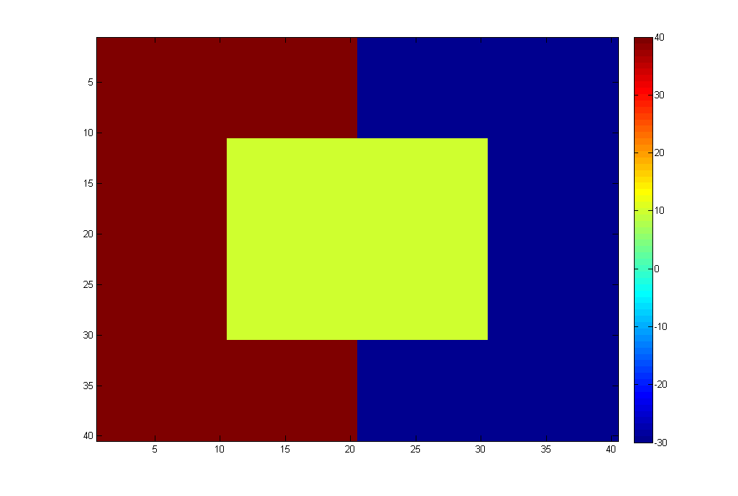
(a)

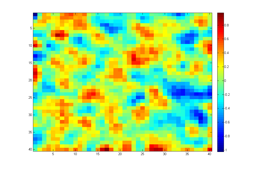
(b)

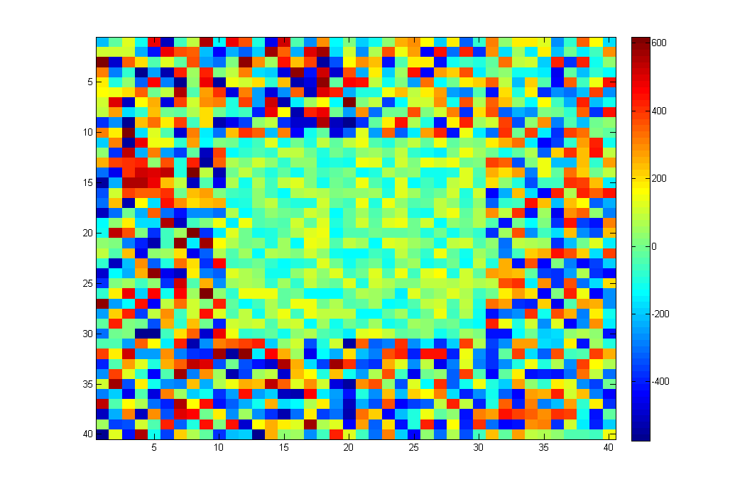
(c)

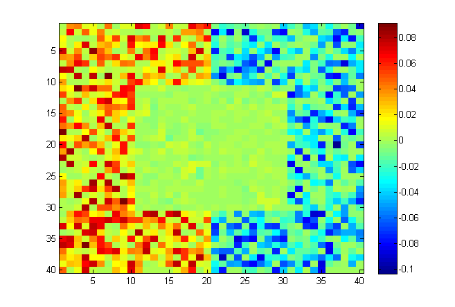
(d)

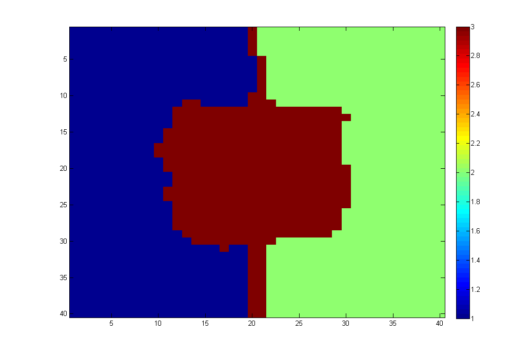
(e)

Figure 1: (a) True $\beta$ values for three regions; (b) Smooth residual effects (c) Y values; (d) dfbetas (e) Detected pattern of $\hat{\beta}$.

Table 1: Summaries of Estimates of $\hat{\beta}^{c}$ in the Simulation Study

	RAR		SAR		CAR
Parameters	Mean (sd)	CI coverage	Mean (sd)	CI coverage	Mean (sd)	CI coverage
			$\sigma^{2}=1$
$\beta^{1}$ (40)	39.00(3.22)	98%	4.19 (0.35)	4.1%	3.35 (0.28)	4.9%
$\beta^{2}$ (-30)	-28.68 (1.93)	99%	-	6.3%	-	5.6%
$\beta^{3}$ (10)	9.78 (0.35)	99%	-	22.3%	-	19.3%
			$\sigma^{2}=10$
$\beta^{1}$ (40)	39.13(2.89)	99%	2.07 (1.12)	1.5%	2.23 (1.54)	1.3%
$\beta^{2}$ (-30)	-29.14 (1.02)	99%	-	4.3%	-	2.7%
$\beta^{3}$ (10)	8.88 (0.35)	98%	-	8.3%	-	5.9%
			$\sigma^{2}=100$
$\beta^{1}$ (40)	39.27(3.14)	99%	1.98 (0.87)	0.9%	0.8 (0.93)	0.4%
$\beta^{2}$ (-30)	-29.32 (1.87)	99%	-	0.2%	-	0.3%
$\beta^{3}$ (10)	8.77 (0.52)	99%	-	2.5%	-	2.1%

4 Data Example: air pollution and cardiovascular disease death rate association study

The 2010 annual circulatory mortality with ICD10 code I00-I99 and annual ambient fine particular matter (PM2.5) for 3109 counties in continental U.S was downloaded from CDC Wonder web portal. The annual mortality rate (per 100,000) was age-adjusted and the reference population was 2000 U.S population. The annual PM2.5 measurement was the average of daily PM2.5 based on 10km grid which were aggregated for each county. The measurement of PM2.5 in 10km grid was from US Environmental Protection Agency (EPA) Air Quality System (AQS) PM2.5 in-situ data and National Aeronautics and Space Administration (NASA) Moderate Resolution Imaging Spectroradiometer (MODIS) aerosol optical depth remotely sensed data. In this dataset, a threshold of 65 micrograms per cubic meter was set to (left) truncate the data to avoid invalid interpolation of grid PM2.5. We use the annual data set for 2001, because the population size and demographic information is more accurate by using 2000 U.S. census data. In figure 2, we illustrate the maps for annual age adjusted cardiovascular disease rate and air pollution (PM 2.5) level.

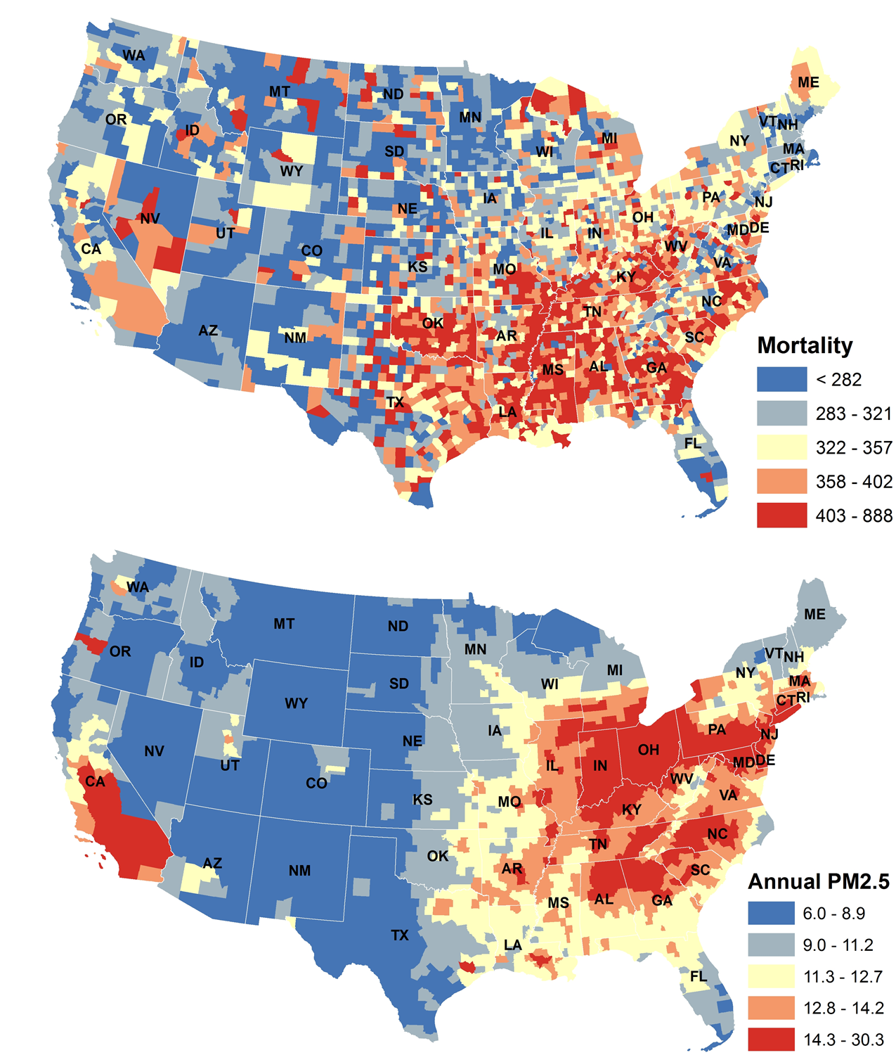
Figure 2: Air pollution and mortality

We perform the RAR analysis on this data set by following the three steps described in section 2. We select the number of regions $K=16$ which minimizes BIC. We then incorporate the identified region labels as categorical covariates as well as the interaction between region labels and PM2.5 exposure levels. We examine the effects of detected regions (by introducing 15 dummy variables and 15 interaction variables) by using likelihood ratio test, both main effects (region) and interaction terms are significant with $p<0.001$. Figure 3 demonstrates the automatically detected regions and spatially varying associations between PM 2.5 and mortality rate at different regions (secondary parameters). The results reveal that the EHA are not coherent across the counties in the nation and RAR defines regions by breaking and rejoining the counties in different states based on similarity of EHA. The RAR defined map may also reveal potential confounders that affect health risk assessment. We note that the most significant positive EHA resides in northwest region and Florida: although the air pollution levels are not among the highest, the disease and exposure are highly positively associated. There are regions exhibiting negative EHA, for instance, the southeast region (part of GA, SC, and NC) and we further verify the association on the exposure and health outcome in enlarged Figure and interestingly by visual checking the exposure and health outcome are negatively associated. There could be potential co-founders such as medical facility accessibility and dietary behavior difference, etc. Our results reveal that region-wise EHA may vary across the nation (affected by local factors), which in part addresses the ecological fallacy (Simpson’s Paradox). The RAR method could be used as a tool to raise further research questions and to motivate new public health research investigation of the variation.

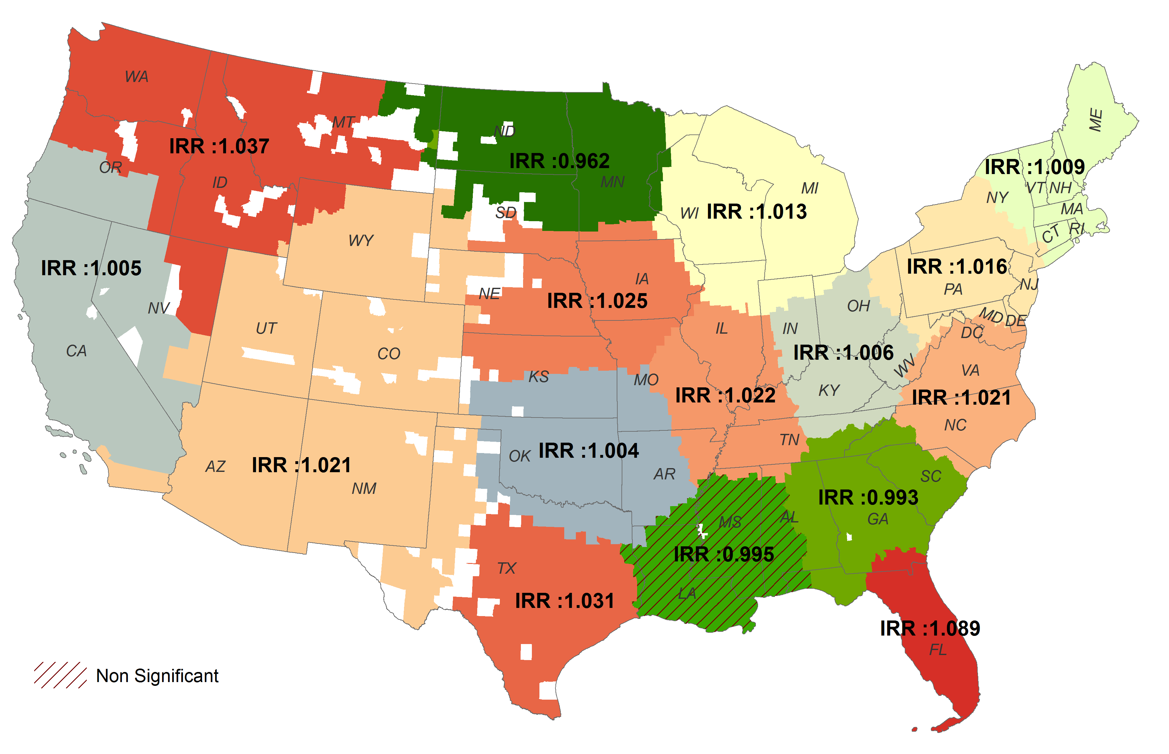
Figure 3: Results: spatially varying associations on RAR detected regions

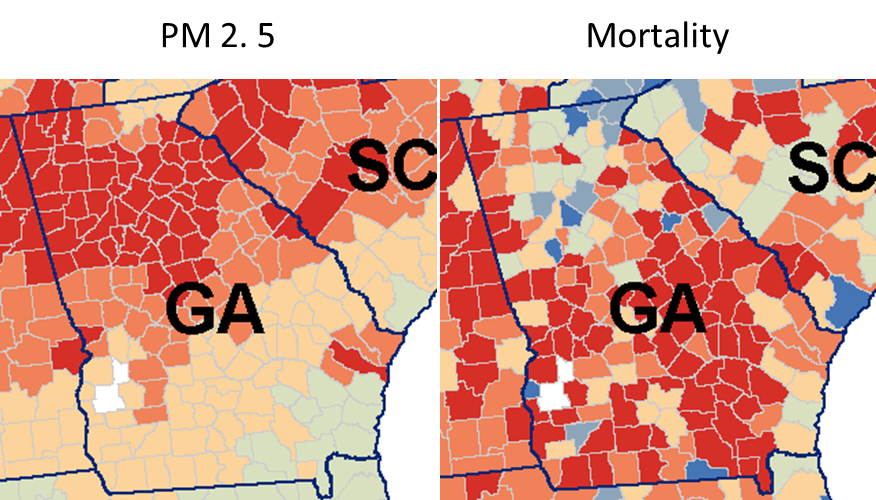
Figure 4: Enlarged exposure and mortality maps to illustrate the negative EHA in the southeast

5 Discussion

The mapping of disease and further building environment-health/disease association have long been a key aspect of public health research. However there has been challenge for statistical data analysis to yield spatially varying EHA at region level. Most previous methods employ random effect model by letting each spatial unit have a random slope and borrow power from neighbors, which is advantageous with regard to improving model fitting and model variance explanation. But, it is also beneficial to provide a map of regions that is defined by EHA similarity because it would allow us to directly draw statistical inferences at the region level as main effects may vary spatially(which is our major motivation to develop the RAR method).

Rooted from image parcellation, the RAR framework aims to parcellate a large map into several contiguous regions with a two-fold goal: i) to define data-driven regions that reveals spatially varying EHA at region level; and ii) to utilize the regions to fit a better regression model. Based on our simulation and example data analysis results, it seems that the performance of the RAR method is satisfactory. A CAR or SAR model could be applied on top of the RAR method, but the RAR could uniquely provide region-wise inferences. The region-wise EHA inferences provide important guidance for public health decision making. For instance, although the exposure levels at California and Ohio River Valley are high, the EHA of these two regions are not among the highest associations. Thus, the RAR model could provide the informative geographic parcellations and inferences that neither exposure or health status data alone can exhibit (e.g Figure 2).

Clustering and cluster analysis have been widely applied in spatial data analysis (Waller,, 2015). However, the most methods are limited to provide disjoint and contiguous regions with distinct disease exposure associations. The regions with different associations may suggest some unidentified confounders and other public health or geographic/environmental factors affecting population health. Although we demonstrate our model for cross sectional analysis, a longitudinal model could be extended straightforwardly because the DFBETAs could be computed for GEE or mixed effect model as well. The computational load of the RAR model is negligible and all of our simulation and data example calculation time is within a minute by using a PC with i7 CPU and 24G memory.

Appendix

Algorithm:
Given an adjacency matrix $W_{s}$ for each subject $s$ and the number of classes $K$,

1. Compute the degree matrix $D_{s}$, where $D_{s}(i,i)=\sum_{j=1}^{N}W_{s}(i,j)$.

2. Find the eigen-solutions $[V_{s},L_{s}]$ of $D_{s}^{-\frac{1}{2}}W_{s}D_{s}^{-\frac{1}{2}}$ , i.e., solving $D_{s}^{-\frac{1}{2}}W_{s}D_{s}^{-\frac{1}{2}}V_{s}=V_{s}L_{s}$ and $V_{s}V_{s}=I_{N}$. Then compute $Z_{s}=D_{s}^{-\frac{1}{2}}V_{s}$.

3. Normalize $Z_{s}$ by setting $X_{s}={\mathrm{diag}}^{-1}[{\mathrm{diag}}(Z_{s}Z_{s}^{T})]Z_{s}$, where operation $\mathrm{diag}(A)$ extracts the diagonal elements of matrix $A$ as a vector; and $\mathrm{diag}^{-1}(a)$ creates a matrix with diagonal elements equal to $a$ and off-diagonal being zeros.

4. Set the convergence criterion parameter $\rho^{*}=0$, and initialize a $K\times K$ matrix $R_{s}$ by the following steps: denote by $R_{s}^{k}$ the $k$th column of $R_{s}$ for $k=1,\ldots,K$. Set $R^{1}_{s}=[X_{s}(i,1),\ldots,X_{s}(i,K)]^{\mathrm{T}}$, where $i$ is randomly selected from $\{1,\ldots,N\}$. We denote the first column of $R_{s}$ as $R_{s}^{1}$ and the $k_{th}$ column as $R_{s}^{k}$. Then update the rest of the columns by following.
   For $k=2,\ldots,K$, iteratively update $R^{k}_{s}=[X_{s}(i_{k},1),\ldots,X_{s}(i_{k},K)]^{\mathrm{T}}$ where

   $$i_{k}=\operatorname*{arg\,min}_{i\in\{1,\ldots,N\}}c_{k-1}(i),\mbox{ and }c_{k-1}=\sum_{l=1}^{k-1}|X_{s}R_{s}^{l}|.$$

5. Minimize the objective function: $\sum_{s}||Y-X_{s}R_{s}||^{2}=||Y-\widehat{XR}||^{2}$.
   where $||\cdot||$ stands for Frobenius norm; and $\widehat{XR}=\sum_{s}t_{s}X_{s}R_{s}$ with

   $$t_{s}=\frac{1/||X_{s}R_{s}-XcRc||^{2}}{\sum_{s}1/||X_{s}R_{s}-XcRc||^{2}}.$$

   The term $XcRc$ is the centroid of $X_{s}R_{s}$ which minimizes $\sum_{s^{\prime}\neq s}||X_{s}R_{s}-X_{s^{\prime}}R_{s^{\prime}}||^{2}$ with respect to $X_{s^{\prime}}R_{s^{\prime}}$.

   Then $Y(i,l)=1$, where $l=\operatorname*{arg\,max}_{k\in\{1,...,K\}}\widehat{XR}(i,k),\ \>i\in\{1,...,N\}\ and\ l\in\{1,...,K\}$.

6. Conduct singular value decomposition on the matrix $Y^{T}X_{s}$
   $Y^{T}X_{s}=U_{s}\Omega_{s}{V_{s}}^{T}$
   $\rho=\sum_{s}tr(\Omega_{s})$
   If $|\rho-\rho^{*}|<\text{pre-assigned error limit then output}\>Y$,
   else, update $R_{s}=V_{s}U_{s}^{T}$.

7. Go to Step 5.

References

- Banerjee et al., (2004) Banerjee, S., Gelfand, A. E., Carlin, B. P. (2004). Hierarchical modeling and analysis for spatial data. Crc Press, Boca Raton, FL.
- Banerjee et al., (2008) Banerjee, S., Gelfand, A. E., Finley, A. O., Sang, H. (2008). Gaussian predictive process models for large spatial data sets. Journal of the Royal Statistical Society: Series B (Statistical Methodology), 70(4), 825-848.
- Bell et al., (2014) Bell, M. L., Ebisu, K., Leaderer, B. P., Gent, J. F., Lee, H. J., Koutrakis, P., … Peng, R. D. (2014). Associations of PM2. 5 constituents and sources with hospital admissions: analysis of four counties in Connecticut and Massachusetts (USA) for persons 65 years of age. Environmental health perspectives, 122(2), 138.
- Besag, (1974) Besag, J. (1974). “Spatial interaction and the statistical analysis of lattice systems (with discussion).” Journal of the Royal Statistical Society - Series B, 36: 192-236.
- Besag, (1986) Besag, J. E. (1986), On the statistical analysis of dirty pictures (with discussion), Journal of the Royal Statistical Society, Ser. B., 48, 259-302.
- Besag et al., (1991) Besag, J., York, J. Molle, A. (1991). Bayesian image restoration with two applications in spatial statistics. Annals of the Institute of Statistics and Mathematics 43, 1–59.
- Best et al., (1999) Best, N., Arnold, R.A., Thomas, A., Waller, L.A., and Conlon, E.M. (1999) Bayesian models for spatially correlated disease and exposure data. In Bayesian Statistics 6, J.M. Bernardo, J.O. Berger, A.P., Dawid, and A.F.M. Smith (eds.). Oxford: Oxford University Press.
- Chung, (1997) Chung, F. R. (1997). Spectral graph theory (Vol. 92). American Mathematical Society.
- Chung et al., (2015) Chung, Y., Dominici, F., Wang, Y., Coull, B. A., Bell, M. L. (2015). Associations between long-term exposure to chemical constituents of fine particulate matter (PM2. 5) and mortality in Medicare enrollees in the Eastern United States. Environmental health perspectives, 123(5), 467.
- Cressie and Wikle, (2011) Cressie, N. and Wikle, C. (2011), Statistics for Spatio-Temporal Data, Hoboken, NJ: Wiley.
- Dominici et al., (2002) Dominici, F., Daniels, M., Zeger, S. L., Samet, J. M. (2002). Air pollution and mortality: estimating regional and national dose-response relationships. Journal of the American Statistical Association, 97(457), 100-111.
- Gelfand and Vounatsou, (2003) Gelfand, A. E., Vounatsou, P. (2003). Proper multivariate conditional autoregressive models for spatial data analysis. Biostatistics, 4(1), 11-15.
- Gelfand et al., (2003) Gelfand, A. E., Kim, H. J., Sirmans, C. F., Banerjee, S. (2003). Spatial modeling with spatially varying coefficient processes. Journal of the American Statistical Association, 98(462), 387-396.
- Garcia et al., (2015) Garcia, C. A., Yap, P. S., Park, H. Y., Weller, B. L. (2015). Association of long-term PM2. 5 exposure with mortality using different air pollution exposure models: impacts in rural and urban California. International journal of environmental health research, (ahead-of-print), 1-13.
- Hodges, (2003) Hodges, J. S., Carlin, B. P., Fan, Q. (2003). On the precision of the conditionally autoregressive prior in spatial models. Biometrics, 59(2), 317–322.
- Hughes, (2013) Hughes, J. and Haran, M. (2013). Dimension reduction and alleviation of confounding for spatial generalized linear mixed models. Journal of the Royal Statistical Society, Series B, 75, 139–159.
- Lawson, (2013) Lawson, A. B. (2013). Bayesian disease mapping: hierarchical modeling in spatial epidemiology. CRC Press, Boca Raton, FL.
- Lei and Rinaldo, (2014) Lei, J., Rinaldo, A. (2014). Consistency of spectral clustering in stochastic block models. The Annals of Statistics, 43(1), 215–237.
- Lu and Carlin, (2005) Lu, H., Carlin, B. P. (2005). Bayesian areal wombling for geographical boundary analysis. Geographical Analysis, 37(3), 265-285.
- Ma and Carlin, (2007) Ma, H., Carlin, B. P. (2007). Bayesian multivariate areal wombling for multiple disease boundary analysis. Bayesian analysis, 2(2), 281-302.
- Ma and Carlin, (2010) Ma, H., Carlin, B. P., Banerjee, S. (2010). Hierarchical and Joint Site‐Edge Methods for Medicare Hospice Service Region Boundary Analysis. Biometrics, 66(2), 355-364.
- Ng et al., (2002) Ng, A. Y., Jordan, M. I., Weiss, Y. (2002). On spectral clustering: Analysis and an algorithm. Advances in neural information processing systems, 2, 849-856.
- Preisser and Qaqish, (1996) Preisser, J. S. and Qaqish, B. F. (1996), Deletion Diagnostics for Generalised Estimating Equations, Biometrika, 83, 551–562.
- Shi et al., (2000) Shi, J., and Malik, J. (2000). Normalized cuts and image segmentation. Pattern Analysis and Machine Intelligence, IEEE Transactions on, 22(8), 888-905.
- Von Luxburg, (2007) Von Luxburg, U. (2007). A tutorial on spectral clustering. Statistics and computing, 17(4), 395-416.
- Von Luxburg et al., (2008) Von Luxburg, U., Belkin, M., Bousquet, O. (2008). Consistency of spectral clustering. The Annals of Statistics, 555-586.
- Waller et al., (2007) Waller, L. A., Goodwin, B. J., Wilson, M. L., Ostfeld, R. S., Marshall, S. L., Hayes, E. B. (2007). Spatio-temporal patterns in county-level incidence and reporting of Lyme disease in the northeastern United States, 1990–2000. Environmental and Ecological Statistics, 14(1), 83-100.
- Waller and Gotway, (2004) Waller, L. A., Gotway, C. A. (2004). Spatial Data. Applied Spatial Statistics for Public Health Data, Hoboken NJ, Wiley.
- Waller, (2015) Waller, L. A. (2015). Discussion: Statistical Cluster Detection, Epidemiologic Interpretation, and Public Health Policy. Statistics and Public Policy, 2(1), 1-8.
- Wheeler et al., (2008) Wheeler, D. C. and Waller, L. A. (2008). Mountains, valleys, and rivers: the transmission of raccoon rabies over a heterogeneous landscape. Journal of agricultural, biological, and environmental statistics, 13(4), 388-406.
- Williams, (1987) Williams, D. A. (1987), Generalized Linear Model Diagnostics Using the Deviance and Single Case Deletions, Applied Statistics, 36, 181-191.
- Womble, (1951) Womble, W. H. (1951). “Differential systematics.” Science, 114: 315–322.
- Yu and Shi, (2003) Yu, Stella X., and Jianbo Shi. ”Multiclass spectral clustering.” In Computer Vision, 2003. Proceedings. Ninth IEEE International Conference on, pp. 313-319. IEEE, 2003.
- Zhu et al., (2014) Zhu, H., Fan, J. and Kong, L. (2014). Spatially Varying Coefficient Model for Neuroimaging Data with Jump Discontinuities. Journal of the American Statistical Association, in press.