Fast multilevel solvers for a class of discrete fourth order parabolic problems

Abstract

In this paper, we study fast iterative solvers for the solution of fourth order parabolic equations discretized by mixed finite element methods. We propose to use consistent mass matrix in the discretization and use lumped mass matrix to construct efficient preconditioners. We provide eigenvalue analysis for the preconditioned system and estimate the convergence rate of the preconditioned GMRes method. Furthermore, we show that these preconditioners only need to be solved inexactly by optimal multigrid algorithms. Our numerical examples indicate that the proposed preconditioners are very efficient and robust with respect to both discretization parameters and diffusion coefficients. We also investigate the performance of multigrid algorithms with either collective smoothers or distributive smoothers when solving the preconditioner systems.

1 Introduction

Fourth order parabolic partial differential equations (PDEs) appear in many applications including the lubrication approximation for viscous thin films king2003fourth , interface morphological changes in alloy systems during stress corrosion cracking by surface diffusion asaro1972interface , image segmentation, noise reduction, inpainting bertozzi2007inpainting ; greer2004h , and phase separation in binary alloys blowey1991cahn ; elliott1989cahn ; cahn2004free , etc. There have been extensive studies on the numerical methods for solving these fourth order parabolic PDEs, including the finite difference methods furihata2001stable ; sun1995second , spectral methods ye2005fourier ; he2008stability , discontinuous Galerkin methods xia2007local ; choo2005discontinuous ; feng2007fully , $\displaystyle C^{1}$-conforming finite element methods elliott1987numerical ; feng2005numerical , nonconforming finite element methodselliott1989nonconforming ; zhang2010nonconforming , and mixed finite element methods du1991numerical ; elliott1989second ; elliott1992error ; feng2004error ; barrett1999finite ; BElliot1992Cahn-Hilliard . The resulting large sparse linear systems of equations are typically very ill-conditioned which poses great challenges for designing efficient and robust iterative solvers. In addition, the linear systems become indefinite when mixed methods are employed. In this work, we design fast iterative solvers for the fourth order parabolic equations discretized by mixed finite element methods.

Multigrid (MG) methods are among the most efficient and robust solvers for solving the linear systems arising from the discretizations of PDEs. There have been a number of studies on multigrid methods for fourth order parabolic equations kay2006multigrid ; Kim2004 ; wise2007solving ; banas2009multigrid ; henn2005multigrid . It is known that smoothers play a significant role in multigrid algorithms. In particular, for saddle point systems, there are two different types of smoothers, i.e., decoupled or coupled smoothers. For a decoupled point smoother, each sweep consists of relaxation over variables per grid point as well as relaxation over grid points. On the other hand, for a coupled point smoother, variables on each grid point are relaxed simultaneously which corresponds to solving a sequence of local problems. Distributive Gauss-Seidel (DGS) is the first decoupled smoother proposed by Brandt and Dinar brandt1979multi for solving Stokes equations. Later, Wittum wittum1999multigrid introduced transforming smoothers and combined it with incomplete LU factorization to solve saddle-point systems with applications in Stokes and Navier-Stokes equations. Gaspar, Lisbona, Oosterlee and Wienands gaspar2004systematic studied the DGS smoother for solving poroelasticity problems. Recently, Wang and Chen wang2013multigrid proposed a distributive Gauss-Seidel smoother based on the least squares commutator for solving Stokes equations and showed multigrid uniform convergence numerically. For coupled smoother, in Vanka1986block , Vanka proposed a symmetrically coupled Gauss-Seidel smoother for the Navier-Stokes equations discretized by finite difference schemes on staggered grids. Later, in Olshanskii2002 , Olshanskii and Reusken introduced an MG solver with collective smothers for the Navier-Stokes equations in rotation form discretized by conforming finite elements. They proved that W-cycle MG method with block Richardson smoother is robust for the discrete problem. Their numerical experiments show that the W-cycle MG method with the damped Jacobi smoother is robust with respect to the mesh size and problem parameters. Collective Jacobi and Gauss-Seidel smoothers have also been studied in multigrid method for elliptic optimal control problems by Lass, Vallejos, Borzi and Douglas Lass2009 , and Takacs and Zulehner Takacs2011 . In our work, we investigate the performance of both coupled and decouple smoothers for the discrete fourth order problem in the mixed form.

In the literature, there are also many studies on the Krylov subspace methods and their preconditioners for solving fourth order parabolic problems. In bansch2004surface ; bansch2005finite , Bänsch, Morin and Nochetto solved a discrete fourth order parabolic equation by applying the conjugate gradient method on the two-by-two block system in Schur complement form. In bansch2011preconditioning , the same authors proposed symmetric and nonsymmetric preconditioners based on operator splitting. Axelsson, Boyanova, Kronbichler, Neytcheva, Do-Quang, and WuAxelsson2011 ; Boyanova2012 ; Axelsson2013 ; Boyanova2014 proposed a block preconditioner by adding an extra small term to the $\displaystyle(2,2)$ block and then followed by a block LU factorization which results in a preconditioned system when eigenvalues have a uniform bound. Bosch, Kay, Stoll, and Wathen Bosch2014a studied block triangular preconditioner for the mixed finite element discretization of a modified Cahn-Hilliard equation for binary image inpainting. In their method, the Schur complement is solved by algebraic multigrid method (AMG) using V-cycle and Chebyshev smoother. Moreover, the convergence rate of their method is independent of the mesh size. Same method has been used by Bosch, Stoll, and Benner in Bosch2014b to solve Cahn-Hilliard variational inequalities. Ingraser2007preconditioned , Gräser and Kornhuber introduced a preconditioned Uzawa-type iterative method with multigrid solvers for subproblems to solve Cahn-Hilliard equation with an obstacle potential. Based on the Hermitian and skew-Hermitian splitting (HSS) iteration introduced in bai2003hermitian , Benzi and Golub benzi2004preconditioner proposed a robust preconditioner for the generalized saddle point problems which exhibit similar two-by-two block structure as the discrete fourth order parabolic problems in mixed form. Later, Bai, Benzi, Chen, and Wang Bai:2013aa studied preconditioned modified HSS (PMHSS) iteration methods for the block linear systems. In Bai2013 , Bai, Chen, and Wang further simplified PMHSS and proposed an additive block diagonal preconditioner for a block linear system of equations arising from finite element discretization of two-phase flow problems and elliptic PDE-constrained optimization problems.

In this work, we construct preconditioners for discrete fourth order parabolic problems based on the mass lumping technique. Mass lumping technique has been widely used in solving time dependent PDEs by the finite element method HRZ_1976 . It consists of replacing a consistent mass matrix by a diagonal lumped mass matrix so that its inversion at each time step becomes a simple division. The error estimates for lumped mass approximation have been studied in Ushijima1977 ; ushijima1979error ; chenthomee1985lumped which show that the order of accuracy for the discretization is preserved. On the other hand, the loss of solution accuracy associated with mass lumping has been studied by Gresho, Lee, and Sani gresho1978advection for advection equations and by Niclasen and Blackburn Niclasen1995 for incompressible Navier-Stokes equations. It is well known that mass lumping may also induce dispersion errors when solving wave equations, see e.g., mullen_belytschko_1982 ; mark_christon_1999 . These studies suggest that it is sometimes advantageous to use consistent mass matrix in the discretization schemes. In the study of fourth order parabolic equations, both consistent mass matrix and lumped mass matrix have been widely used. In this work, we choose consistent mass matrix in the finite element discretization to keep the solution accuracy and utilize lumped mass matrix to design efficient preconditioners so that the cost of inverting consistent mass matrix can be alleviated. We prove that GMRes method with mass lumping preconditioner converges when $\displaystyle\tau\geq Ch^{2}$ for some constant $\displaystyle C$ depending on the diffusion coefficients ($\displaystyle\tau$, $\displaystyle h$ corresponds to time and spatial discretization parameters, respectively). In a special case when the two diffusion operators $\displaystyle A$ and $\displaystyle B$ only differ by a scaling factor, we are able to prove uniform convergence of GMRes method for the preconditioned system without the constraint $\displaystyle\tau\geq Ch^{2}$. Furthermore, we show that the preconditioner systems can be solved inexactly by geometric multigrid methods with the two different types of smoother discussed previously. By combining the optimality of multigrid methods with the computational efficiency of the mass lumping technique, we obtain very efficient solvers for the discrete fourth order problems.

The remainder of the paper is organized as follows. In Section 2, we describe the model problem and the corresponding mixed finite element discretization. Next, in Section 3, we describe the multigrid method and the collective Jacobi/Gauss-Seidel smoothers for our model problem. In Section 4, we construct two mass lumping preconditioners. Multigrid method with decoupled smoother are also introduced in this section to solve the preconditioner system approximately. The spectrum bounds of the preconditioned systems and the convergence property of GMRes method are analyzed in Section 5. Finally, in Section 6, we present numerical experiments to demonstrate the efficiency and robustness of the proposed solvers.

2 Model Problem and Discretization

2.1 Model problem

We are interested in solving the following fourth order problem:

$$\displaystyle u-\tau\;\mbox{div}(a\nabla v) \displaystyle=f\ \;\mbox{in}\;\Omega,$$ (2.1)

$$\displaystyle\tau\;\mbox{div}(b\nabla u)+v \displaystyle=g\ \;\mbox{in}\;\Omega,$$ (2.2)

with boundary conditions

$$\displaystyle u=v=0,\quad\mbox{on}\ \Gamma_{D},$$ (2.3)

$$\displaystyle\nu\cdot a\nabla v=\nu\cdot b\nabla u=0,\quad\mbox{on}\ \Gamma_{N}.$$ (2.4)

where $\displaystyle\tau=\sqrt{\triangle t}$ and $\displaystyle\triangle t$ is the time-step size, $\displaystyle\Omega$ is a bounded polyhedral domain in $\displaystyle\mathbb{R}^{d}$, $\displaystyle d\geq 1$, $\displaystyle\nu$ is the unit outward normal, $\displaystyle\Gamma_{D}$, $\displaystyle\Gamma_{N}$ denote the Dirichlet and Neumann boundary part, respectively. We mainly study the Dirichlet boundary condition in this paper, i.e., $\displaystyle\Gamma_{N}=\emptyset$. The diffusion coefficients $\displaystyle a(x)$ and $\displaystyle b(x)$ are measurable functions satisfying the following continuity and coercivity conditions

$$\lambda_{a}(x)|\xi|^{2}\leq\xi^{T}a(x)\xi\leq\Lambda_{a}(x)|\xi|^{2},\quad\lambda_{b}(x)|\xi|^{2}\leq\xi^{T}b(x)\xi\leq\Lambda_{b}(x)|\xi|^{2},\;\forall\xi\in\mathbb{R}^{d}.$$

Eqns (2.1) and (2.2) may arise from a time semi-discretization of the fourth order parabolic problem

$$u_{t}=\mbox{div}(a\nabla(-\mbox{div}(b\nabla u))).$$

In this case, $\displaystyle f=u^{\text{old}}$ is the solution at the previous time step, and $\displaystyle g=0$.

As an example, consider the following Cahn-Hilliard equations that model the phase separation and coarsening dynamics in a binary alloy:

$$u_{t}-\mbox{div}(M(u)\nabla(-\epsilon\Delta u+F^{\prime}(u)))=0,\;\mbox{in}\;\Omega\times(0,T),$$ (2.5)

where $\displaystyle\Omega\subset\mathbb{R}^{3}$ is a bounded domain, $\displaystyle u$ represents the relative concentration of one component in a binary mixture, $\displaystyle M(u)$ is the degenerate mobility, which restricts diffusion of both components to the interfacial region, e.g., $\displaystyle M(u)=u(1-u)$ barrett1999finite , $\displaystyle F^{\prime}(u)$ is the derivative of a double well potential $\displaystyle F(u)$, a typical choice is

$$F(u)=\frac{1}{4}(u^{2}-1)^{2}.$$

Introducing $\displaystyle v$, defined by $\displaystyle v=\tau(-\epsilon\Delta u+F^{\prime}(u))$(the chemical potential multiplied by $\displaystyle\tau$), after semi-implicit time discretization, we obtain a splitting of (2.5) into a coupled system of second order equations elliott1989second ; elliott1992error ; feng2004error

$$\displaystyle u-\tau\mbox{div}(M(u)\nabla v) \displaystyle=f,\;\mbox{in}\;\Omega,$$

$$\displaystyle\tau(-\epsilon\Delta u+F^{\prime}(u))-v \displaystyle=0,\;\mbox{in}\;\Omega.$$

Denote $\displaystyle a=M(u)$, $\displaystyle b=\epsilon$, and assume $\displaystyle F^{\prime}(u)=0$, we can get (2.1) and (2.2), which corresponds to the linearization of the nonlinear Cahn-Hilliard equations.

The weak formulation of (2.1)-(2.2) is: find $\displaystyle u,v\in\mathbb{V}$ such that

$$\begin{array}[]{ccc}(u,\phi)+\tau(a\nabla v,\nabla\phi)&=&(f,\phi),\quad\phi\in\mathbb{V}\\ -\tau(b\nabla u,\nabla\psi)+(v,\psi)&=&(g,\psi),\quad\psi\in\mathbb{V},\end{array}$$ (2.6)

where $\displaystyle\mathbb{V}$ is the subspace of $\displaystyle H^{1}(\Omega)$ associated with the boundary condition (2.3). The well-posedness of (2.6) follows from the Lax-Milgram lemma quarteroni1980mixed .

2.2 Finite element discretization

Let $\displaystyle\mathcal{T}$ be a shape-regular triangulation of $\displaystyle\Omega$, $\displaystyle\mathbb{V}_{\mathcal{T}}$ be the piecewise linear finite element space over $\displaystyle\mathcal{T}$ satisfying the homogeneous boundary condition (2.3), and $\displaystyle N_{h}={\rm dim(\mathbb{V}_{\mathcal{T}})}$. The discrete problem for the PDE system (2.1)-(2.2) is: find $\displaystyle u_{h},v_{h}\in\mathbb{V}_{\mathcal{T}}$, such that $\displaystyle\forall\phi,\psi\in\mathbb{V}_{\mathcal{T}}$

$$\begin{array}[]{ccc}(u_{h},\phi)+\tau(a\nabla v_{h},\nabla\phi)&=&(f,\phi),\\ -\tau(b\nabla u_{h},\nabla\psi)+(v_{h},\psi)&=&(g,\psi).\end{array}$$

In matrix form, we have

$$\left(\begin{array}[]{rc}\tau A&M\\ M&-\tau B\end{array}\right)\left(\begin{array}[]{c}\utilde{v}\\ \utilde{u}\end{array}\right)=\left(\begin{array}[]{r}\utilde{f}\\ \utilde{g}\end{array}\right),\;\;\text{or}\;\;\mathcal{A}\left(\begin{array}[]{c}\utilde{v}\\ \utilde{u}\end{array}\right)=\left(\begin{array}[]{r}\utilde{f}\\ \utilde{g}\end{array}\right),$$ (2.7)

where $\displaystyle\mathcal{A}$ is a matrix of size $\displaystyle 2N_{h}\times 2N_{h}$, $\displaystyle M$ is the mass matrix, and $\displaystyle A$, $\displaystyle B$ are the stiffness matrices defined by

$$M_{i,j}=(\phi_{i},\phi_{j}),\quad A_{i,j}=(a\nabla\phi_{i},\nabla\phi_{j}),\quad B_{i,j}=(b\nabla\phi_{i},\nabla\phi_{j}).$$

Eliminating $\displaystyle\utilde{v}$ in (2.7), we get the following Schur complement equation

$$(M+\tau^{2}AM^{-1}B)\utilde{u}=\utilde{f}-\tau AM^{-1}\utilde{g}.$$ (2.8)

In this paper, we develop efficient preconditioners for the two-by-two block linear systems (2.7); however, we will solve the Schur complement for preconditioners. In order to avoid inverting mass matrix, we employ the mass lumping technique to construct preconditioners.

3 Multigrid with Collective Smoother

A multigrid algorithm typically consists of three major components: the smoother (or relaxation scheme), the coarse grid operator, and the grid transfer operators (interpolation/restriction operators). It is well known that the efficiency of a multigrid method crucially depends on the choice of the smoother. In particular, for the block system (2.7), we observe numerically that multigrid method with point-wise Gauss-Seidel smoother does not converge uniformly. We construct a block Jacobi or Gauss-Seidel smoother that collects the degrees of freedom corresponding to variables $\displaystyle u$ and $\displaystyle v$ for each grid point. In other words, each block corresponds to a $\displaystyle 2\times 2$ matrix.

To describe these collective smoothers, we first consider the following matrix splitting, i.e.,

$$\mathcal{A}=\mathcal{A}_{L}+\mathcal{A}_{D}+\mathcal{A}_{L}^{T},\;\;\mathcal{A}_{L}=\left(\begin{array}[]{cc}\tau L_{A}&L_{M}\\ L_{M}&-\tau L_{B}\end{array}\right),\;\;\mathcal{A}_{D}=\left(\begin{array}[]{cc}\tau D_{A}&D_{M}\\ D_{M}&-\tau D_{B}\end{array}\right),$$

where $\displaystyle L_{A},L_{B},L_{M}$ are strictly lower triangular parts of $\displaystyle A$, $\displaystyle B$, and $\displaystyle M$, and $\displaystyle D_{A},D_{B},D_{M}$ are their diagonal parts. The collective damped Jacobi relaxation can be represented as

$$\displaystyle\begin{pmatrix}\utilde{v}^{k+1}\\ \utilde{u}^{k+1}\end{pmatrix}=\begin{pmatrix}\utilde{v}^{k}\\ \utilde{u}^{k}\end{pmatrix}+\vartheta\mathcal{A}_{D}^{-1}\left[\begin{pmatrix}\utilde{f}\\ \utilde{g}\end{pmatrix}-\mathcal{A}\begin{pmatrix}\utilde{v}^{k}\\ \utilde{u}^{k}\end{pmatrix}\right]$$ (3.1)

The collective Gauss-Seidel relaxation can be represented as

$$\displaystyle\begin{pmatrix}\utilde{v}^{k+1}\\ \utilde{u}^{k+1}\end{pmatrix}=\begin{pmatrix}\utilde{v}^{k}\\ \utilde{u}^{k}\end{pmatrix}+(\mathcal{A}_{L}+\mathcal{A}_{D})^{-1}\left[\begin{pmatrix}\utilde{f}\\ \utilde{g}\end{pmatrix}-\mathcal{A}\begin{pmatrix}\utilde{v}^{k}\\ \utilde{u}^{k}\end{pmatrix}\right]$$ (3.2)

More practically, one can rearrange variables $\displaystyle\utilde{u}$ and $\displaystyle\utilde{v}$ in $\displaystyle\utilde{w}$ so that $\displaystyle\mathcal{A}_{L}+\mathcal{A}_{D}$ corresponds to a lower block triangular matrix. In fact, let $\displaystyle\utilde{w}=(\utilde{w}_{1},\utilde{w}_{2},\dots,\utilde{w}_{N_{h}})^{T}$ with each entry $\displaystyle\utilde{w}_{i}=(v_{i},u_{i})$ corresponds to a pair of variables. Then, each relaxation sweep of (3.1) consists of solving a sequence of small systems

$$\displaystyle\utilde{w}_{i}^{k+1}=\utilde{w}^{k}_{i}+\vartheta\mathscr{A}^{-1}_{ii}\left(F_{i}-\sum_{j=1}^{N_{h}}\mathscr{A}_{ij}\utilde{w}^{k}_{j}\right),$$

and each sweep of (3.2) consists of solving

$$\displaystyle\utilde{w}_{i}^{k+1}=\utilde{w}^{k}_{i}+\mathscr{A}^{-1}_{ii}\left(F_{i}-\sum_{j=1}^{i-1}\mathscr{A}_{ij}\utilde{w}^{k+1}_{j}-\sum_{j=i}^{N_{h}}\mathscr{A}_{ij}\utilde{w}^{k}_{j}\right),$$

where

$$\mathscr{A}_{ij}=\begin{pmatrix}\tau A_{ij}&M_{ij}\\ M_{ij}&-\tau B_{ij}\end{pmatrix},\;\;F_{i}=\begin{pmatrix}f_{i}\\ g_{i}\end{pmatrix},\quad i,j=1,2,\cdots,N_{h}.$$

Note that $\displaystyle\mathscr{A}_{ii}$ is invertible since $\displaystyle\text{det}(\mathscr{A}_{ii})=-\tau^{2}A_{ii}B_{ii}-M_{ii}^{2}\neq 0$.

It is clear from the above form that for collective damped Jacobi relaxation, these small system can be solved in parallel, and for collective Gauss-Seidel relaxation, they are solved successively. Numerical experiments in Section 6 indicate that by relaxing both variables $\displaystyle u_{i},v_{i}$ corresponding to the same grid point $\displaystyle i$ collectively, geometric multigrid V-cycle converges uniformly with respect to both $\displaystyle h$ and $\displaystyle\tau$.

The collective Gauss-Seidel smoother has been studied by Lass, Vallejos, Borzi and Douglas in Lass2009 for solving elliptic optimal control problems. It is shown in Lass2009 that the convergence rate of multigrid method with collective Gauss-Seidel smoother is independent of $\displaystyle h$. The robustness with respect to $\displaystyle\tau$ is, however, hard to prove theoretically. Takacs and Zulehner Takacs2011 also investigated multigrid algorithm with several collective smoothers for optimal control problems and proved the convergence of the W-cycle multigrid with collective Richardson smoother. For convergence proof of multigrid methods using collective smoothers applied to saddle point systems, we refer to the work by Schöberl Schoberl:1999aa and by Chen Chen:aa ; Chen:2015aa .

4 Mass Lumping Preconditioners

In this section, we study preconditioners for the two-by-two block linear systems (2.7) for use with GMRes method. When the meshsize and time-step size are small, these systems are generally very ill-conditioned, especially when the diffusion coefficients $\displaystyle a$ and $\displaystyle b$ degenerate. Hence, efficient preconditioners are necessary in order to speed up the convergence of GMRes method. In bansch2011preconditioning , Bänsch, Morin, and Nochetto proposed symmetric and non-symmetric preconditioners that work well for the Schur complement system (2.8). However, the convergence rates of these methods are not uniform with respect to $\displaystyle h$ or $\displaystyle\tau$. Besides, the performance of those methods deteriorate for degenerate problems bansch2011preconditioning .

In the following, we design two preconditioners based on the mass lumping technique and geometric multigrid method for the system (2.7). The main focus is on the efficiency and robustness of the proposed solvers. Numerical experiments in Section 6 indicate that GMRes method preconditioned by the mass lumping preconditioners (solved inexactly) converges uniformly with respect to the discretization parameters and is also robust for problems with degenerate diffusion coefficients.

4.1 Preconditioner with two lumped mass matrices

The mass lumping technique has been widely used in the finite element computations, especially for time-dependent problems as it avoids inverting a full mass matrix $\displaystyle M$ at each time step. The lumped-mass matrix $\displaystyle\bar{M}$ is a diagonal matrix with diagonal elements equal to the row sums of $\displaystyle M$. By using the diagonal matrix $\displaystyle\bar{M}$, the computational cost for the preconditioner is reduced significantly.

The mass lumping preconditioner $\displaystyle\mathcal{B}$ for the block system $\displaystyle\mathcal{A}$ is defined by

$$\mathcal{B}=\begin{pmatrix}\tau A&\bar{M}\\ \bar{M}&-\tau B\end{pmatrix}.$$ (4.1)

GMRes method is then applied to solve the preconditioned linear system

$$\begin{pmatrix}\tau A&{M}\\ {M}&-\tau B\end{pmatrix}\begin{pmatrix}\tau A&\bar{M}\\ \bar{M}&-\tau B\end{pmatrix}^{-1}\left(\begin{array}[]{c}\utilde{p}\\ \utilde{q}\end{array}\right)=\left(\begin{array}[]{c}\utilde{f}\\ \utilde{g}\end{array}\right).$$ (4.2)

4.2 Preconditioner with one lumped mass matrix

We can also use the following preconditioner $\displaystyle\tilde{\mathcal{B}}$ with one lumped mass matrix for solving the block system (2.7), i.e.

$$\tilde{\mathcal{B}}=\begin{pmatrix}\tau A&{M}\\ \bar{M}&-\tau B\end{pmatrix}.$$ (4.3)

The matrix $\displaystyle\tilde{\mathcal{B}}$ is nonsymmetric and is a better approximation to $\displaystyle\mathcal{A}$ compared with $\displaystyle\mathcal{B}$. For $\displaystyle\tilde{\mathcal{B}}$, we still have a block factorization which avoids inverting mass matrix $\displaystyle M$. Numerical experiments of Section 6.2 indicate that the performance of the two preconditioners $\displaystyle\tilde{\mathcal{B}}$ and $\displaystyle\mathcal{B}$ used with GMRes method are similar when solved inexactly by geometric multigrid V-cycle when $\displaystyle\tau\geq Ch^{2}$. However, when $\displaystyle\tau$ is very small, $\displaystyle\tilde{\mathcal{B}}$ performs better than $\displaystyle\mathcal{B}$.

4.3 Multigrid for Preconditioners

The preconditioner systems only need to be solved approximately. We can use geometric multigrid method with the coupled smoothers described in Section 3. In the following, we construct a decoupled smoother following the idea of the distributive Gauss-Seidel relaxation (DGS) which is suitable for the model problem.

DGS is a decoupled smoother introduced by Brandt in brandt1979multi for solving Stokes equations. The main idea of DGS is to apply standard Gauss-Seidel relaxation on decoupled equations using transformed variables. Let us consider the mass-lumping preconditioner system $\displaystyle\tilde{\mathcal{B}}$ (a similar scheme can be derived for $\displaystyle\mathcal{B}$),

$$\tilde{\mathcal{B}}\left(\begin{array}[]{c}\utilde{v}\\ \utilde{u}\end{array}\right)=\left(\begin{array}[]{c}\utilde{p}\\ \utilde{q}\end{array}\right).$$ (4.4)

We introduce the following change of variables

$$\left(\begin{array}[]{c}\utilde{v}\\ \utilde{u}\end{array}\right)=\mathcal{P}\left(\begin{array}[]{c}\utilde{x}\\ \utilde{y}\end{array}\right),\;\;\text{where}\;\;\mathcal{P}=\left(\begin{array}[]{cc}\tau\bar{M}^{-1}B&0\\ I&I\end{array}\right)$$ (4.5)

is called the distribution matrix. Right preconditioning $\displaystyle\tilde{\mathcal{B}}$ by $\displaystyle\mathcal{P}$ results in an upper block triangular matrix

$$\displaystyle\tilde{\mathcal{B}}\mathcal{P}=\left(\begin{array}[]{cc}M+\tau^{2}A\bar{M}^{-1}B&M\\ 0&-\tau B\end{array}\right).$$

We construct a decoupled smoother for preconditioner (4.4) by solving

$$\begin{pmatrix}\utilde{v}^{k+1}\\ \utilde{u}^{k+1}\end{pmatrix}=\begin{pmatrix}\utilde{v}^{k}\\ \utilde{u}^{k}\end{pmatrix}+\mathcal{P}(\tilde{\mathcal{B}}\mathcal{P})^{-1}\left[\begin{pmatrix}\utilde{p}\\ \utilde{q}\end{pmatrix}-\tilde{\mathcal{B}}\begin{pmatrix}\utilde{v}^{k}\\ \utilde{u}^{k}\end{pmatrix}\right]$$ (4.6)

More precisely, we have the following algorithm

1. Form the residual: $$\displaystyle\begin{pmatrix}\utilde{r}_{v}\\ \utilde{r}_{u}\end{pmatrix}=\left[\begin{pmatrix}\utilde{p}\\ \utilde{q}\end{pmatrix}-{\tilde{\mathcal{B}}}\begin{pmatrix}\utilde{v}^{k}\\ \utilde{u}^{k}\end{pmatrix}\right]$$ 2. Apply standard Gauss-Seidel relaxation to solve the error equation $$\displaystyle-\tau B\utilde{e}_{y}=\utilde{r}_{u}$$ and use the damped Jacobi relaxation for $$(M+\tau^{2}A\bar{M}^{-1}B)\utilde{e}_{x}=\utilde{r}_{v}-M\utilde{e}_{y}.$$ (4.7) Then, recover $\displaystyle\utilde{e}_{u},\utilde{e}_{v}$ from (4.5), i.e., $\displaystyle\displaystyle\utilde{e}_{v}$ $\displaystyle\displaystyle=\tau\bar{M}^{-1}B\utilde{e}_{x};$ $\displaystyle\displaystyle\utilde{e}_{u}$ $\displaystyle\displaystyle=\utilde{e}_{x}+\utilde{e}_{y}$ 3. Update the solution $$\begin{array}[]{cc}\utilde{v}^{k+1}=\utilde{v}^{k}+\utilde{e}_{v}\\ \utilde{u}^{k+1}=\utilde{u}^{k}+\utilde{e}_{u}\end{array}$$

We can use multigrid method with the above decoupled smoother to solve the preconditioner system (4.4).

Remark 1

By using the damped Jacobi to solve (4.7), we can avoid matrix multiplication. In fact, we only need to calculate the diagonal part of $\displaystyle M+\tau^{2}A\bar{M}^{-1}B$. This requires $\displaystyle\mathcal{O}(N_{h})$ operations because $\displaystyle\bar{M}$ is a diagonal matrix.

5 Convergence Analysis of Preconditioned GMRes Method

In this section, we analyze the convergence of the GMRes method preconditioned by the two preconditioners introduced in Section 4 for the block system (2.7). We show that the preconditioned GMRes method converges when $\displaystyle\tau\geq Ch^{2}$ for some constant $\displaystyle C$ depending on the diffusion coefficients. Numerical results in Section 6 indicate that the preconditioned GMRes method converges uniformly for any $\displaystyle h$ and $\displaystyle\tau$.

Let $\displaystyle R=\mathcal{A}\mathcal{B}^{-1}$ (or $\displaystyle\mathcal{A}\tilde{\mathcal{B}}^{-1}$) with $\displaystyle\mathcal{B}$ (or $\displaystyle\tilde{\mathcal{B}}$) being a right preconditioner of $\displaystyle\mathcal{A}$. To solve the preconditioned system $\displaystyle Rv=b$, the GMRes method starts from an initial iterate $\displaystyle v_{0}$ and produces a sequence of iterates $\displaystyle v_{k}$ and residuals $\displaystyle r_{k}:=b-Rv_{k}$, such that $\displaystyle r_{k}=p_{k}(R)r_{0}$ for some polynomial $\displaystyle p_{k}\in\mathcal{P}_{k}$, and

$$\|r_{k}\|_{2}=\min_{\begin{subarray}{c}p\in\mathcal{P}_{k}\\ p(0)=1\end{subarray}}\|p(R)r_{0}\|_{2},$$ (5.1)

where $\displaystyle\mathcal{P}_{k}$ is the space of polynomials of degree $\displaystyle k$ or less and $\displaystyle\|\cdot\|_{2}$ is the Euclidean norm. As a consequence, the convergence rate of the GMRes method can be estimated by

$$\frac{\|r_{k}\|_{2}}{\|r_{0}\|_{2}}\leq\min_{\begin{subarray}{c}p\in\mathcal{P}_{k}\\ p(0)=1\end{subarray}}\|p(R)\|_{2}.$$ (5.2)

Since $\displaystyle R$ may not be a normal matrix, we follow the approach given in bansch2011preconditioning using the concept of $\displaystyle\epsilon$-pseudospectrum trefethen2005spectra . Given $\displaystyle\epsilon>0$, denote by $\displaystyle\sigma_{\epsilon}(R)$ the set of $\displaystyle\epsilon$-eigenvalues of $\displaystyle R$, namely those $\displaystyle z\in\mathbb{C}$ that are eigenvalues of some matrix $\displaystyle R+E$ with $\displaystyle\|E\|\leq\epsilon$. We first quote the following two results.

Lemma 1 (Pseudospectrum estimate trefethen2005spectra )

Let $\displaystyle\Sigma_{\epsilon}$ be a union of closed curves enclosing the $\displaystyle\epsilon-$pseudospectrum $\displaystyle\sigma_{\epsilon}(R)$ of $\displaystyle R$. Then for any polynomial $\displaystyle p_{k}$ of degree $\displaystyle k$ with $\displaystyle p_{k}(0)=1$ we have

$$\max_{z\in\sigma(R)}|p_{k}(z)|\leq\|p_{k}(R)\|\leq\frac{L_{\epsilon}}{2\pi\epsilon}\max_{z\in\Sigma_{\epsilon}(R)}|p_{k}(z)|,$$ (5.3)

where $\displaystyle L_{\epsilon}$ is the arclength of $\displaystyle\Sigma_{\epsilon}$.

Lemma 2 (Bound on the $\displaystyle\epsilon$-pseudospectrum bansch2011preconditioning )

If $\displaystyle R$ is a square matrix of order $\displaystyle n$ and $\displaystyle 0<\epsilon\leq 1$, then,

$$\sigma_{\epsilon}(R)\subset\cup_{\lambda\in\sigma(R)}B(\lambda,C_{R}\epsilon^{\frac{1}{m}}),$$

where $\displaystyle C_{R}:=n(1+\sqrt{n-p})\kappa(V)$, with $\displaystyle\kappa(V)$ the condition number of $\displaystyle V$ and $\displaystyle V$ is a nonsingular matrix transforming $\displaystyle R$ into its Jordan canonical form $\displaystyle J$, i.e. $\displaystyle V^{-1}RV=J$, $\displaystyle p$ is the number of Jordan blocks, and $\displaystyle m$ is the size of the largest Jordan block of $\displaystyle R$.

In order to estimate the error caused by mass lumping, we introduce the following operators chenthomee1985lumped . Let $\displaystyle z_{j}(1\leq j\leq 3)$ be the vertices of a triangle $\displaystyle K\in\mathcal{T}$, consider the following quadrature formula

$$\displaystyle Q_{K,h}(f) \displaystyle=\sum_{j=1}^{3}(1,\phi_{j}|_{K})f(z_{j})=\frac{1}{3}|K|\sum_{j=1}^{3}f(z_{j})$$

$$\displaystyle(\phi_{i},\phi_{j})_{h} \displaystyle=\sum_{K\in\mathcal{T}}Q_{K,h}(\phi_{i}\phi_{j})=\int_{\Omega}\pi_{h}(\phi_{i}\phi_{j})dx$$

where $\displaystyle\pi_{h}:C^{0}(\bar{\Omega})\rightarrow\mathbb{V}_{\mathcal{T}}$ is the standard nodal interpolation operator. Then, the mass lumping procedure can be interpreted as

$$(\phi_{j},\phi_{j})_{h}=Q_{K,h}(\phi_{j}\phi_{j})=\sum_{k=1}^{N_{h}}(\phi_{j},\phi_{k}).$$

The following results are useful for later analysis.

Lemma 3 (quadrature error chenthomee1985lumped )

Let $\displaystyle u,v\in\mathbb{V}_{\mathcal{T}}\subset H_{0}^{1}$ and $\displaystyle(u,v)_{h}$ be the lumped inner product. Then,

$$\displaystyle|(u,v)-(u,v)_{h}|\leq C_{l}h^{2}|u|_{1}|v|_{1},$$ (5.4)

where $\displaystyle C_{l}$ is a constant independent of $\displaystyle h$.

Lemma 4 (Norm equivalence elliott1989second )

Let $\displaystyle M$ be the mass matrix and $\displaystyle\bar{M}$ be its lumped version. Then, for any $\displaystyle u=\textstyle{\sum}_{j}u_{j}\phi_{j}\in\mathbb{V}_{\mathcal{T}}$ we have

$$C_{1}(\bar{M}\utilde{u},\utilde{u})\leq(M\utilde{u},\utilde{u})\leq(\bar{M}\utilde{u},\utilde{u}),$$ (5.5)

where $\displaystyle\utilde{u}=(u_{1},u_{2},\cdots,u_{N_{h}})^{T}$ and $\displaystyle C_{1}\in(0,1)$ is a constant independent of $\displaystyle h$.

Proof

We first show that $\displaystyle({M}\utilde{u},\utilde{u})\leq(\bar{M}\utilde{u},\utilde{u})$. Let $\displaystyle\delta M=M-\bar{M}$, then

$$(\delta M)_{ij}<0,\ i=j;\quad(\delta M)_{ij}\geq 0,\ i\neq j;\ \ {\rm and}\ \ (\delta M)_{ii}=-\sum_{j\neq i}(\delta M)_{ij}.$$

By direct calculations, we have

$$\displaystyle{\utilde{u}}^{T}\delta M\utilde{u} \displaystyle= \displaystyle\sum_{i=1}^{N_{h}}\sum_{j=1}^{N_{h}}(\delta M)_{ij}u_{i}u_{j}$$

$$\displaystyle= \displaystyle\sum_{i=1}^{N_{h}}\left({u}_{i}\sum_{j<i}(\delta M)_{ij}({u}_{j}-{u}_{i})+{u}_{i}\sum_{j>i}(\delta M)_{ij}({u}_{j}-{u}_{i})\right)$$

$$\displaystyle= \displaystyle\sum_{i=1}^{N_{h}}\sum_{j>i}-(\delta M)_{ij}({u}_{j}-{u}_{i})^{2}\leq 0.$$

By Lemma 3 and the inverse inequality, we get

$$\displaystyle(u,u)_{h}-(u,u) \displaystyle\leq|(u,u)-(u,u)_{h}|\leq C_{l}h^{2}|u|_{1}^{2}\leq C\|u\|_{0}^{2}=C(u,u).$$

Hence, $\displaystyle(u,u)_{h}\leq(1+C)(u,u)$. Equivalently,

$$\frac{1}{1+C}(\bar{M}\utilde{u},\utilde{u})\leq(M\utilde{u},\utilde{u})$$

which implies that the left inequality holds with $\displaystyle C_{1}={1}/({1+C})$ for some positive constant $\displaystyle C$.

We also need the following estimates for the eigenvalues of the stiffness matrices and mass matrix fried1973bounds , brenner2008book .

Lemma 5 (Eigenvalue estimates)

Let $\displaystyle A,B$ be the stiffness matrices corresponding to diffusion coefficients $\displaystyle a(x)$ and $\displaystyle b(x)$, respectively, and let $\displaystyle M$ be the mass matrix, then,

$$\displaystyle\lambda_{\max}(A)\leq C_{A},\quad\lambda_{\max}(B)\leq C_{B},\quad C_{M}h^{2}\leq\lambda_{\min}(M)$$ (5.6)

where $\displaystyle C_{A},C_{B}$ depend on the continuity assumption of the bilinear forms and the constant in the inverse inequality.

5.1 Eigenvalue analysis for $\displaystyle\mathcal{A}\mathcal{B}^{-1}$ with constraint $\displaystyle\tau\geq Ch^{2}$

Recall

$$\displaystyle\mathcal{B}=\begin{pmatrix}\tau A&\bar{M}\\ \bar{M}&-\tau B\end{pmatrix},\quad\mathcal{A}=\begin{pmatrix}\tau A&M\\ M&-\tau B\end{pmatrix}.$$

We have the following spectrum bound for the preconditioned system $\displaystyle\mathcal{B}^{-1}\mathcal{A}$.

Theorem 5.1 (Spectral bound for $\displaystyle\mathcal{B}^{-1}\mathcal{A}$)

Let $\displaystyle h$ denote the meshsize and $\displaystyle\tau$ denote the square root of time-step size. Then, the spectral radius of $\displaystyle\mathcal{B}^{-1}\mathcal{A}$ satisfies

$$\rho(\mathcal{B}^{-1}\mathcal{A})<2,$$

if $\displaystyle{\tau}\geq Ch^{2}$ for some positive constant $\displaystyle C$ independent of $\displaystyle h$ and $\displaystyle\tau$.

Proof

Let $\displaystyle\lambda\in\mathbb{C},\ (\utilde{v},\utilde{u})^{T}\in\mathbb{C}^{2N_{h}}$ be a pair of eigenvalue and eigenvector of $\displaystyle\mathcal{B}^{-1}\mathcal{A}$, i.e.

$$\displaystyle\begin{pmatrix}\tau A&\bar{M}\\ \bar{M}&-\tau B\end{pmatrix}^{-1}\begin{pmatrix}\tau A&{M}\\ {M}&-\tau B\end{pmatrix}\begin{pmatrix}\utilde{v}\\ \utilde{u}\end{pmatrix}=\lambda\begin{pmatrix}\utilde{v}\\ \utilde{u}\end{pmatrix}.$$

Equivalently,

$$\begin{pmatrix}\tau A&{M}\\ {M}&-\tau B\end{pmatrix}\begin{pmatrix}\utilde{v}\\ \utilde{u}\end{pmatrix}=\lambda\begin{pmatrix}\tau A&\bar{M}\\ \bar{M}&-\tau B\end{pmatrix}\begin{pmatrix}\utilde{v}\\ \utilde{u}\end{pmatrix}.$$ (5.7)

Taking the inner product of the equation (5.7) with $\displaystyle(\utilde{v}^{T},-\utilde{u}^{T})$, we obtain

$$[\tau(A\utilde{v},\utilde{v})+\tau(B\utilde{u},\utilde{u})+2\imath{\rm{Im}}(M\utilde{v},\utilde{u})]=\lambda[\tau(A\utilde{v},\utilde{v})+\tau(B\utilde{u},\utilde{u})+2\imath{\rm{Im}}(\bar{M}\utilde{v},\utilde{u})].$$ (5.8)

Then, we have

$$2\imath{\rm Im}(\delta M\utilde{v},\utilde{u})=(\lambda-1)[\tau(A\utilde{v},\utilde{v})+\tau(B\utilde{u},\utilde{u})+2\imath{\rm{Im}}(\bar{M}\utilde{v},\utilde{u})].$$ (5.9)

Since $\displaystyle A$ and $\displaystyle B$ are symmetric positive definite matrices, $\displaystyle\|\utilde{v}\|^{2}_{A}=(A\utilde{v},\utilde{v})$ and $\displaystyle\|\utilde{u}\|^{2}_{B}=(B\utilde{u},\utilde{u})$ are nonnegative real numbers. By taking the modulus of (5.9) we get

$$4|{\rm Im}(\delta M\utilde{v},\utilde{u})|^{2}=|\lambda-1|^{2}(\alpha^{2}+4|{\rm Im}(\bar{M}\utilde{v},\utilde{u})|^{2}),$$

where $\displaystyle\alpha=\tau(\|\utilde{v}\|_{A}^{2}+\|\utilde{u}\|_{B}^{2})$. Hence,

$$|\lambda-1|^{2}=\frac{4|{\rm Im}(\delta M\utilde{v},\utilde{u})|^{2}}{\alpha^{2}+4|{\rm{Im}}(\bar{M}\utilde{v},\utilde{u})|^{2}}.$$ (5.10)

Let $\displaystyle v={\textstyle\sum}_{i}v_{i}\phi_{i}$, $\displaystyle u={\textstyle\sum}_{i}u_{i}\phi_{i}$, we get

$$\displaystyle|(\delta M\utilde{v},\utilde{u})| \displaystyle\leq \displaystyle C_{l}h^{2}|v|_{1}|u|_{1}\quad\text{(by (\ref{property3-M}))}$$

$$\displaystyle\leq \displaystyle C_{l}C_{a}C_{b}h^{2}\|\utilde{v}\|_{A}\|\utilde{u}\|_{B}\quad(C_{a}=\min_{x}\lambda_{a}(x),\ C_{b}=\min_{x}\lambda_{b}(x))$$

$$\displaystyle\leq \displaystyle C_{l}C_{a}C_{b}h^{2}\frac{\|\utilde{v}\|_{A}^{2}+\|\utilde{u}\|^{2}_{B}}{2}\quad\text{(by Young's inequality)}$$

$$\displaystyle= \displaystyle\frac{C_{l}C_{a}C_{b}h^{2}}{2\tau}\tau\left(\|\utilde{v}\|_{A}^{2}+\|\utilde{u}\|^{2}_{B}\right),$$

Hence,

$$\displaystyle 4{\rm Im}|(\delta M\utilde{v},\utilde{u})|^{2}\leq\frac{(C_{l}C_{a}C_{b})^{2}h^{4}}{\tau^{2}}\tau^{2}(\|\utilde{v}\|_{A}^{2}+\|\utilde{u}\|_{B}^{2})^{2}=\frac{(C_{l}C_{a}C_{b})^{2}h^{4}}{\tau^{2}}\alpha^{2}.$$

Let $\displaystyle C=2C_{l}C_{a}C_{b}$, when $\displaystyle\tau\geq Ch^{2}$, we get $\displaystyle\rho(\mathcal{B}^{-1}\mathcal{A})<2$.

Using the same proof of Corollary 5.11 in bansch2011preconditioning with $\displaystyle\epsilon_{0}={1-\rho(\mathcal{B}^{-1}\mathcal{A})/2}$, we have

Corollary 1 (Convergence rate of GMRes for $\displaystyle\mathcal{A}\mathcal{B}^{-1}$)

For the preconditioned system $\displaystyle\mathcal{A}\mathcal{B}^{-1}$, GMRes method converges with an asymptotic linear convergence rate bounded by

$$\theta=\frac{\rho(\mathcal{B}^{-1}\mathcal{A})}{2},$$

if $\displaystyle\tau\geq Ch^{2}$. Moreover,

$$\frac{\|r_{k}\|_{2}}{\|r_{0}\|_{2}}\leq C_{0}\theta^{k},$$

with $\displaystyle C_{0}=2^{m-1}C_{R}^{m}(1+\rho(E)){\rm dim}\mathbb{V}_{\mathcal{T}}/(1-\rho(E))^{m}$, $\displaystyle C_{R},\ m$ are the parameters defined in the Lemma 2 and $\displaystyle\mathbb{V}_{\mathcal{T}}$ is the finite element space.

Similarly, we have the following result.

Corollary 2 (Convergence rate of GMRes for $\displaystyle\mathcal{A}\tilde{\mathcal{B}}^{-1}$)

The spectral radius of $\displaystyle\tilde{\mathcal{B}}^{-1}\mathcal{A}$ satisfies

$$\rho(\tilde{\mathcal{B}}^{-1}\mathcal{A})<2,$$

if $\displaystyle{\tau}\geq Ch^{2}$ for some constant $\displaystyle C$ independent with $\displaystyle h$ and $\displaystyle\tau$. For the preconditioned system $\displaystyle\mathcal{A}\tilde{\mathcal{B}}^{-1}$, GMRes method converges with an approximate linear convergence rate bounded by

$$\tilde{\theta}=\frac{\rho(\tilde{\mathcal{B}}^{-1}\mathcal{A})}{2}.$$

5.2 Analysis without the constraint $\displaystyle\tau\geq Ch^{2}$

As we will see in Section 6, numerical results show uniform convergence rate of GMRes method for the preconditioned system irrespective of the relation between $\displaystyle h$ and $\displaystyle\tau$. A proof of this result appears elusive due to the fact that the Schur complement is nonsymmetric. In this subsection, we give a proof in this direction for the special case $\displaystyle B=\alpha A$ with $\displaystyle\alpha>0$ being some scaling constant in the mass lumping preconditioner $\displaystyle\tilde{\mathcal{B}}$. For simplicity, we choose $\displaystyle\alpha=1$ for the remaining part of this paper.

Notice that

$$\begin{pmatrix}\tau A&M\\ \bar{M}&-\tau B\end{pmatrix}^{-1}=\begin{pmatrix}I&-(\tau A)^{-1}M\\ 0&I\end{pmatrix}\begin{pmatrix}(\tau A)^{-1}&0\\ 0&(-\tau B-\bar{M}(\tau A)^{-1}M)^{-1}\end{pmatrix}\begin{pmatrix}I&0\\ -\bar{M}(\tau A)^{-1}&I\end{pmatrix}$$

$$\displaystyle\tilde{\mathcal{B}}^{-1}\mathcal{A} \displaystyle=\begin{pmatrix}\tau A&M\\ \bar{M}&-\tau B\end{pmatrix}^{-1}\begin{pmatrix}\tau A&{M}\\ M&-\tau B\end{pmatrix}=\begin{pmatrix}I+X&0\\ (-\tau B-\bar{M}(\tau A)^{-1}M)^{-1}({M}-\bar{M})&I\end{pmatrix},$$

where

$$X=(\tau A)^{-1}M(\tau B+\bar{M}(\tau A)^{-1}M)^{-1}({M}-\bar{M}).$$

Then, any eigenvalue of $\displaystyle\tilde{\mathcal{B}}^{-1}\mathcal{A}$ is either 1 or $\displaystyle 1+\lambda$ for some $\displaystyle\lambda\in\sigma(X)$ where $\displaystyle\sigma(X)$ represents the spectrum of $\displaystyle X$.

To derive the bounds of $\displaystyle\sigma(X)$, we first recall the Sherman-Morrison-Woodbury formula

$$(A+UV^{T})^{-1}=A^{-1}-A^{-1}U(I+V^{T}A^{-1}U)^{-1}V^{T}A^{-1},$$

and the following identity

$$V^{T}(A+UV^{T})^{-1}U=(I+(V^{T}A^{-1}U)^{-1})^{-1}.$$ (5.11)

Appying (5.11), we get

$$\displaystyle X \displaystyle=(\tau A)^{-1}M(\tau B+\bar{M}(\tau A)^{-1}M)^{-1}\bar{M}[\bar{M}^{-1}({M}-\bar{M})]$$

$$\displaystyle=\left[I+((\tau A)^{-1}M(\tau B)^{-1}\bar{M})^{-1}\right]^{-1}(\bar{M}^{-1}M-I)$$

$$\displaystyle=\left(I+\tau^{2}(A^{-1}MB^{-1}\bar{M})^{-1}\right)^{-1}(\bar{M}^{-1}M-I)$$

$$\displaystyle=\left(I+\tau^{2}\bar{M}^{-1}BM^{-1}A\right)^{-1}(\bar{M}^{-1}M-I).$$

Lemma 6 (Spectrum of X)

If $\displaystyle A=B$, and $\displaystyle C_{1}<1$ is the constant in (5.5), then

$$\sigma(X)\subset(C_{1}-1,0].$$

Proof

Let $\displaystyle(\lambda,\utilde{w})$ be an eigenpair of the matrix $\displaystyle X$, then

$$\displaystyle X\utilde{w}=\lambda\utilde{w} \displaystyle\Leftrightarrow \displaystyle(\bar{M}^{-1}M-I)\utilde{w}=\lambda(I+\tau^{2}\bar{M}^{-1}AM^{-1}A)\utilde{w}$$

$$\displaystyle\Leftrightarrow \displaystyle(M-\bar{M})\utilde{w}=\lambda(\bar{M}+\tau^{2}AM^{-1}A)\utilde{w}$$

$$\displaystyle\Leftrightarrow \displaystyle\lambda=\frac{((M-\bar{M})\utilde{w},\utilde{w})}{((\bar{M}+\tau^{2}AM^{-1}A)\utilde{w},\utilde{w})}$$

$$\displaystyle\Leftrightarrow \displaystyle 0\geq\lambda>(C_{1}-1)\frac{(\bar{M}\utilde{w},\utilde{w})}{(\bar{M}\utilde{w},\utilde{w})+(\tau^{2}AM^{-1}A\utilde{w},\utilde{w})}$$

$$\displaystyle\Leftrightarrow \displaystyle C_{1}-1<\lambda\leq 0.$$

By Lemma 6 and the relation between $\displaystyle\tilde{\mathcal{B}}^{-1}\mathcal{A}$ and $\displaystyle X$, we obtain the following result.

Theorem 5.2 (Spectrum of $\displaystyle\tilde{\mathcal{B}}^{-1}\mathcal{A}$)

Let $\displaystyle\mathcal{A}$ and $\displaystyle\tilde{\mathcal{B}}$ be given by (2.7) and (4.3), respectively. If $\displaystyle A=B$, we have

$$\sigma(\tilde{\mathcal{B}}^{-1}\mathcal{A})\subset(C_{1},1].$$

The following result can be proved by using the same proof for the Corollary 5.11 in bansch2011preconditioning with $\displaystyle\epsilon_{0}=C_{1}/2$.

Corollary 3 (Convergence rate of GMRes for $\displaystyle\mathcal{A}\tilde{\mathcal{B}}^{-1}$)

GMRes’s iteration converges for system $\displaystyle\mathcal{A}\tilde{\mathcal{B}}^{-1}$ with an asymptotic linear convergence rate bounded by

$$\theta=\frac{1-C_{1}/2}{1+C_{1}},$$

Moreover,

$$\frac{\|r_{k}\|}{\|r_{0}\|}\leq C_{0}\theta^{k},$$

with $\displaystyle C_{0}=2^{2m-1}C^{m}_{R}{\rm dim}\mathbb{V}_{\mathcal{T}}/C_{1}^{m-1}$.

Remark 2 (Preconditioning for $\displaystyle\tau<Ch^{2}$)

By inverse inequality, we have $\displaystyle\tau\|u\|_{A}^{2}\leq\tau h^{-2}\|u\|_{M}^{2}$. So if $\displaystyle\tau<h^{2}$, then $\displaystyle M$ will dominate $\displaystyle A$. For the case when $\displaystyle A\neq\alpha B$ and $\displaystyle\tau<Ch^{2}$, we rewrite the system in the following form

$$\begin{pmatrix}M&\tau A\\ -\tau B&M\end{pmatrix}\begin{pmatrix}\utilde{u}\\ \utilde{v}\end{pmatrix}=\begin{pmatrix}\utilde{f}\\ \utilde{g}\end{pmatrix},$$ (5.12)

and consider the diagonal preconditioner

$$\mathcal{B}_{d}=\begin{pmatrix}M&0\\ 0&M\end{pmatrix}.$$ (5.13)

To give an estimate of the spectrum bound for the preconditioned system, we let

$$\begin{pmatrix}M&0\\ 0&M\end{pmatrix}^{-1}\begin{pmatrix}M&\tau A\\ -\tau B&M\end{pmatrix}=I+E_{d}$$

where

$$E_{d}=\begin{pmatrix}M&0\\ 0&M\end{pmatrix}^{-1}\begin{pmatrix}0&\tau A\\ -\tau B&0\end{pmatrix}$$ (5.14)

Let $\displaystyle\left(\lambda,(\utilde{x}^{T},\utilde{y}^{T})\right)$ be an eigenpair of $\displaystyle E_{d}$, i.e.,

$$\begin{pmatrix}0&\tau A\\ -\tau B&0\end{pmatrix}\begin{pmatrix}\utilde{x}\\ \utilde{y}\end{pmatrix}=\lambda\begin{pmatrix}M&0\\ 0&M\end{pmatrix}\begin{pmatrix}\utilde{x}\\ \utilde{y}\end{pmatrix}$$

Taking the inner product of the above equation with the vector $\displaystyle(\utilde{x}^{T},\utilde{y}^{T})$ we obtain

$$(\tau A\utilde{y},\utilde{x})-(\tau B\utilde{x},\utilde{y})=\lambda\left[(M\utilde{x},\utilde{x})+(M\utilde{y},\utilde{y})\right].$$

Denote $\displaystyle\|\cdot\|_{M}^{2}=(M\cdot,\cdot)$, we have

$$|\lambda|=\frac{\tau\left|(A\utilde{y},\utilde{x})-(B\utilde{x},\utilde{y})\right|}{\|\utilde{x}\|^{2}_{M}+\|\utilde{y}\|^{2}_{M}}$$

Since $\displaystyle M$ is symmetric positive definite,

$$\displaystyle|(A\utilde{y},\utilde{x})| \displaystyle\leq \displaystyle\left|(M^{-\frac{1}{2}}AM^{-\frac{1}{2}}M^{\frac{1}{2}}\utilde{y},M^{\frac{1}{2}}\utilde{x})\right|$$

$$\displaystyle\leq \displaystyle\|M^{-\frac{1}{2}}AM^{-\frac{1}{2}}\|\|\utilde{y}\|_{M}\|\utilde{x}\|_{M}$$

$$\displaystyle\leq \displaystyle\|M^{-\frac{1}{2}}AM^{-\frac{1}{2}}\|\frac{\|\utilde{x}\|^{2}_{M}+\|\utilde{y}\|^{2}_{M}}{2}.$$

Similarly,

$$|(B\utilde{x},\utilde{y})|\leq\|M^{-\frac{1}{2}}BM^{-\frac{1}{2}}\|\frac{\|\utilde{x}\|^{2}_{M}+\|\utilde{y}\|^{2}_{M}}{2}$$

Then, by Lemma 5,

$$\displaystyle|\lambda| \displaystyle\leq\frac{\tau}{2}(\|M^{-\frac{1}{2}}AM^{-\frac{1}{2}}\|+\|M^{-\frac{1}{2}}BM^{-\frac{1}{2}}\|)$$

$$\displaystyle\leq\frac{\tau}{2}\left(\frac{\lambda_{\max}(A)}{\lambda_{\min}(M)}+\frac{\lambda_{\max}(B)}{\lambda_{\min}(M)}\right)$$

$$\displaystyle\leq\frac{\tau}{2}\left(\frac{C_{A}}{C_{M}h^{2}}+\frac{C_{B}}{C_{M}h^{2}}\right)=\frac{\tau(C_{A}+C_{B})}{2C_{M}h^{2}}<1,$$

if $\displaystyle\tau<Ch^{2}$, where $\displaystyle C=2C_{M}/(C_{A}+C_{B})$. Hence, all the eigenvalues of the preconditioned system can be bounded in $\displaystyle B(1,\rho(E_{d}))$ with $\displaystyle\rho(E_{d})<1$.

6 Numerical Experiments

In this section, we provide numerical experiments to demonstrate the performance of multigrid method and the preconditioned flexible GMRes method (without restart) using mass lumping preconditioners. The MATLAB adaptive finite element package $\displaystyle i$FEM long2009ifem is used for all experiments. We choose the following two test problems from bansch2011preconditioning .

Consider the L-shaped domain $\displaystyle\Omega=(-1,1)^{2}\backslash[0,1)^{2}$, set $\displaystyle g=0$, $\displaystyle f=1$, and choose the Dirichlet boundary condition in both examples. For the diffusion coefficients $\displaystyle a(x_{1},x_{2}),\ b(x_{1},x_{2})$, we choose

1. Nice problem:

   $$a(x_{1},x_{2})=1,\quad b(x_{1},x_{2})=\left\{\begin{array}[]{cc}0.6,&\mbox{if}\ x_{2}<x_{1},\\ 1.2,&\mbox{otherwise}.\end{array}\right.$$

2. Degenerate problem:

   $$a(x_{1},x_{2})=0.1|x_{1}|+|x_{2}|,\quad b(x_{1},x_{2})=10+3\sin(5\pi x_{1})\sin(8\pi x_{2}).$$

The range of parameter $\displaystyle\tau\in[10^{-4},1]$, which corresponds to the time-step size $\displaystyle\Delta t\in[10^{-8},1]$. The stopping criterion of the multigrid solver and GMRes iteration is chosen to be the relative residual error in $\displaystyle L^{2}$ norm less than $\displaystyle 10^{-7}$. The initial guess for the iterative methods are chosen randomly. For time-dependent problems, we can use the approximation in the previous time step as the initial guess and our solvers can converge in just a few steps. All computations are done using MATLAB R2015b on a desktop computer with a 3.7 GHz Intel processor and 32 GB RAM.

6.1 Results of multigrid solver with collective smoothers

We compare the performance of multigrid method with collective Gauss-Seidel and collective Jacobi smoother (with damping parameter $\displaystyle\vartheta=0.8$) for solving (2.7). We choose this particular Jacobi damping parameter because it gives the best performance compared with other values we have tried. We use multigrid V-cycle with one pre-smoothing and one post-smoothing (i.e., V(1,1)) which achieves the best efficiency in terms of CPU time. The number of iterations and CPU time (in parentheses) are summarized in Tables 6.1 and 6.2. We observe that multigrid methods converge uniformly with respect to $\displaystyle h$. The convergence rate is close to uniform with respect to $\displaystyle\tau$ except for some deterioration when $\displaystyle\tau$ is around $\displaystyle 10^{-4}$ or $\displaystyle 10^{-5}$ as shown in Table 6.1. For very small $\displaystyle\tau$, the block system is dominated by the two mass matrix blocks, and multigrid performs better as shown in Tables 6.1 and 6.2. Although it is not covered by our analysis in Section 5, numerical results in Table 6.2 show that multigrid methods with collective smoothers are robust for problems with degenerate diffusion coefficient.

Table 6.1: Example 1: Iteration counts and CPU time (in seconds) of CGS/CJ-MG

solver	$\displaystyle h$	$\displaystyle\tau$
		1e-0	1e-1	1e-2	1e-3	1e-4	1e-5	1e-6	1e-7
CGS-MG	$\displaystyle 1/64$	8 (0.31)	8 (0.31)	8 (0.31)	8 (0.31)	13 (0.49)	8 (0.31)	7 (0.27)	7 (0.27)
	$\displaystyle 1/128$	8   (1.5)	8   (1.5)	8   (1.5)	8   (1.5)	11 (2.0)	12 (2.2)	7   (1.3)	7   (1.3)
	$\displaystyle 1/256$	8   (6.6)	8   (6.6)	8   (6.6)	8   (6.6)	10 (8.3)	11 (9.1)	9   (7.5)	7   (5.9)
CJ-MG	$\displaystyle 1/64$	15 (0.51)	15 (0.50)	15 (0.51)	15 (0.50)	14 (0.47)	12 (0.40)	13 (0.43)	13 (0.43)
	$\displaystyle 1/128$	15 (2.3)	15 (2.2)	15 (2.2)	15 (2.2)	14 (2.0)	12 (1.8)	13 (1.9)	13 (1.9)
	$\displaystyle 1/256$	15   (10)	15   (10)	15   (10)	15   (10)	15   (10)	14 (9.6)	12 (8.2)	13 (9.0)

Table 6.2: Example 2: Iteration counts and CPU time (in seconds) of CGS/CJ-MG

solver	$\displaystyle h$	$\displaystyle\tau$
		1e-0	1e-1	1e-2	1e-3	1e-4	1e-5	1e-6	1e-7
CGS-MG	$\displaystyle 1/64$	8 (0.31)	8 (0.31)	8 (0.31)	8 (0.31)	10 (0.38)	11 (0.42)	7 (0.27)	7 (0.27)
	$\displaystyle 1/128$	8   (1.5)	8   (1.5)	8   (1.5)	8   (1.5)	8   (1.5)	12   (2.2)	9   (1.7)	7   (1.3)
	$\displaystyle 1/256$	8   (6.8)	8   (6.7)	8   (6.7)	8   (6.7)	8   (6.8)	10   (8.4)	12   (10)	7   (5.9)
CJ-MG	$\displaystyle 1/64$	15 (0.53)	15 (0.52)	15 (0.51)	15 (0.54)	14 (0.48)	12 (0.41)	14 (0.48)	13 (0.44)
	$\displaystyle 1/128$	15 (2.2)	15 (2.2)	15 (2.2)	15 (2.2)	14 (2.1)	13 (1.9)	13 (1.9)	14 (2.1)
	$\displaystyle 1/256$	15   (11)	15   (10)	15   (10)	15   (10)	15   (10)	14   (10)	12   (8.3)	14 (8.6)

6.2 Results of GMRes with preconditioners solved inexactly by CGS-MG

In this subsection, we compare the performance of the preconditioned GMRes method using three different preconditioners $\displaystyle V_{\mathcal{B}}(1,1),V_{\tilde{\mathcal{B}}}(1,1),V_{\mathcal{A}}(1,1)$. Here, we use $\displaystyle V_{\mathcal{B}}(1,1),\ V_{\tilde{\mathcal{B}}}(1,1),V_{\mathcal{A}}(1,1)$ to represent the inexact preconditioners corresponding to $\displaystyle\mathcal{B},\tilde{\mathcal{B}}$ and $\displaystyle\mathcal{A}$ respectively. For example, $\displaystyle V_{\mathcal{B}}(1,1)$ is one CGS-MG V-cycle with one pre-smoothing and one post-smoothing. As we can see from Tables 6.3 and 6.4 that GMRes method converges uniformly with respect to both $\displaystyle h$ and $\displaystyle\tau$. The CPU time for GMRes preconditioned by $\displaystyle V_{\mathcal{B}}(1,1)$ is approximately half of the time when preconditioned by $\displaystyle V_{\mathcal{A}}(1,1)$ which clearly demonstrate the efficiency of mass lumping.

Table 6.3: Example 1: Iteration counts and CPU time (in seconds) of GMRes with one V(1,1) CGS-MG

preconditioner	$\displaystyle h$	$\displaystyle\tau$
		1e-0	1e-1	1e-2	1e-3	1e-4
$\displaystyle V_{\mathcal{B}}(1,1)$	$\displaystyle 1/64$	8 (0.16)	8 (0.16)	8 (0.16)	7 (0.14)	12 (0.25)
	$\displaystyle 1/128$	8 (0.76)	8 (0.72)	8 (0.72)	7 (0.63)	8 (0.72)
	$\displaystyle 1/256$	8 (3.5)	8 (3.4)	8 (3.4)	7 (3.0)	7 (3.0)
$\displaystyle V_{\tilde{\mathcal{B}}}(1,1)$	$\displaystyle 1/64$	8 (0.24)	8 (0.21)	8 (0.22)	7 (0.19)	9 (0.24)
	$\displaystyle 1/128$	8 (1.0)	8 (1.0)	8 (0.98)	7 (0.87)	7 (0.86)
	$\displaystyle 1/256$	8 (4.4)	8 (4.4)	8 (4.4)	7 (3.9)	7 (3.9)
$\displaystyle V_{\mathcal{A}}(1,1)$	$\displaystyle 1/64$	8 (0.33)	8 (0.33)	8 (0.34)	8 (0.33)	7 (0.29)
	$\displaystyle 1/128$	8 (1.5)	8 (1.5)	8 (1.5)	8 (1.5)	8 (1.5)
	$\displaystyle 1/256$	8 (6.9)	8 (6.9)	8 (6.9)	7 (6.1)	8 (6.9)

Table 6.4: Example 2: Iteration counts and CPU time (in seconds) of GMRes with one V(1,1) CGS-MG

preconditioner	$\displaystyle h$	$\displaystyle\tau$
		1e-0	1e-1	1e-2	1e-3	1e-4
$\displaystyle V_{\mathcal{B}}(1,1)$	$\displaystyle 1/64$	8 (0.17)	8 (0.17)	8 (0.17)	8 (0.17)	14 (0.30)
	$\displaystyle 1/128$	8 (0.77)	8 (0.73)	8 (0.73)	8 (0.73)	9 (0.82)
	$\displaystyle 1/256$	8 (3.5)	8 (3.4)	8 (3.4)	8 (3.4)	7 (3.0)
$\displaystyle V_{\tilde{\mathcal{B}}}(1,1)$	$\displaystyle 1/64$	8 (0.22)	8 (0.21)	8 (0.21)	8 (0.22)	8 (0.24)
	$\displaystyle 1/128$	8 (1.0)	8 (0.98)	8 (0.98)	8 (0.98)	7 (0.86)
	$\displaystyle 1/256$	8 (4.5)	8 (4.5)	8 (4.5)	8 (4.5)	7 (3.9)
$\displaystyle V_{\mathcal{A}}(1,1)$	$\displaystyle 1/64$	8 (0.32)	8 (0.33)	8 (0.34)	8 (0.33)	9 (0.37)
	$\displaystyle 1/128$	8 (1.5)	8 (1.5)	8 (1.5)	8 (1.5)	8 (1.5)
	$\displaystyle 1/256$	8 (6.9)	8 (6.9)	8 (6.9)	8 (6.9)	8 (6.9)

6.3 Results of GMRes with preconditioners solved inexactly by DGS-MG

In this subsection, we present the numerical results for GMRes method using inexact mass lumping preconditioners $\displaystyle V_{\mathcal{B}}(1,1)$ and $\displaystyle V_{\tilde{\mathcal{B}}}(1,1)$. Namely, the preconditioner systems $\displaystyle\mathcal{B}$ and $\displaystyle\tilde{\mathcal{B}}$ are solved approximately by one multigrid V-cycle using the decoupled smoother proposed in Section 4.3 with one pre-smoothing and one post-smoothing. Here, we choose the Jacobi damping parameter to be $\displaystyle 0.5$. Our numerical experiments show that the preconditioners have similar performance when the Jacobi damping parameter varies between $\displaystyle 0.4$ and $\displaystyle 0.6$. As we can see from Tables 6.5 and 6.6 that GMRes converges uniformly when varying $\displaystyle h$ and $\displaystyle\tau$.

Table 6.5: Example 1: Iteration counts and CPU time (in seconds) of GMRes with one V(1, 1) DGS-MG

preconditioner	$\displaystyle h$	$\displaystyle\tau$
		1e-0	1e-1	1e-2	1e-3	1e-4
$\displaystyle V_{\mathcal{B}}(1,1)$	$\displaystyle 1/64$	22 (0.28)	22 (0.28)	21 (0.26)	19 (0.25)	20 (0.25)
	$\displaystyle 1/128$	22 (1.1)	22 (1.1)	21 (1.1)	20 (1.0)	19 (0.98)
	$\displaystyle 1/256$	22 (5.4)	22 (5.3)	22 (5.3)	21 (5.1)	19 (4.6)
$\displaystyle V_{\tilde{\mathcal{B}}}(1,1)$	$\displaystyle 1/64$	22 (0.29)	22 (0.30)	21 (0.28)	19 (0.25)	17 (0.40)
	$\displaystyle 1/128$	22 (1.2)	22 (1.2)	21 (1.1)	20 (1.1)	19 (1.0)
	$\displaystyle 1/256$	22 (5.5)	22 (5.5)	22 (5.5)	21 (5.2)	19 (4.8)

Table 6.6: Example 2: Iteration counts and CPU time (in seconds) of GMRes with one V(1, 1) DGS-MG

preconditioner	$\displaystyle h$	$\displaystyle\tau$
		1e-0	1e-1	1e-2	1e-3	1e-4
$\displaystyle V_{\mathcal{B}}(1,1)$	$\displaystyle 1/64$	23 (0.29)	22 (0.28)	21 (0.27)	19 (0.24)	20 (0.25)
	$\displaystyle 1/128$	21 (1.1)	22 (1.1)	22 (1.1)	20 (1.0)	18 (0.92)
	$\displaystyle 1/256$	21 (5.0)	21 (5.0)	21 (5.0)	20 (4.8)	18 (4.3)
$\displaystyle V_{\tilde{\mathcal{B}}}(1,1)$	$\displaystyle 1/64$	23 (0.30)	23 (0.30)	22 (0.29)	19 (0.26)	17 (0.23)
	$\displaystyle 1/128$	22 (1.2)	23 (1.2)	22 (1.2)	20 (1.1)	17 (0.94)
	$\displaystyle 1/256$	21 (5.3)	22 (5.5)	21 (5.3)	20 (5.0)	18 (4.5)

6.4 Choice of multigrid parameters for solving preconditioner systems

In the following, we compare the performance of the preconditioner $\displaystyle\mathcal{B}$ solved by CGS-MG or DGS-MG with different types of cycles and different number of smoothing steps. From Tables 6.7 - 6.10, we can see that increasing the number of smoothing steps can reduce the number of GMRes iterations. However, the CPU time is not always decreasing since more smoothing steps may also increase the computational cost. The GMRes iteration numbers are similar when using W cycle or V cycle. Since W cycle is usually more expensive, its efficiency in terms of CPU time is not as good as V cycle in our experiment. For practical purposes, we suggest using V cycle with one pre- and one post-smoothing step for solving the preconditioner systems discussed in this work.

Table 6.7: Example 1: Iteration count, CPU time (in seconds), and convergence factor (italics) of GMRes preconditioned by one $\displaystyle V_{\mathcal{B}}(k,k)$ CGS-MG, $\displaystyle k=1,2,3$

precond	$\displaystyle h$	$\displaystyle\tau$
		1e-0	1e-1	1e-2	1e-3	1e-4
$\displaystyle V_{\mathcal{B}}(1,1)$	$\displaystyle 1/64$	8 (0.16)	8 (0.16)	8 (0.16)	7 (0.14)	12 (0.25)
		0.09	0.09	0.09	0.10	0.23
	$\displaystyle 1/128$	8 (0.76)	8 (0.72)	8 (0.72)	7 (0.63)	8 (0.72)
		0.09	0.09	0.09	0.10	0.12
	$\displaystyle 1/256$	8 (3.5)	8 (3.4)	8 (3.4)	7 (3.0)	7 (3.0)
		0.09	0.09	0.09	0.09	0.10
$\displaystyle V_{\mathcal{B}}(2,2)$	$\displaystyle 1/64$	6 (0.14)	6 (0.14)	5 (0.12)	6 (0.14)	11 (0.26)
		0.09	0.09	0.09	0.10	0.23
	$\displaystyle 1/128$	6 (0.67)	6 (0.63)	5 (0.53)	5 (0.53)	6 (0.63)
		0.09	0.09	0.09	0.10	0.12
	$\displaystyle 1/256$	6 (3.1)	6 (3.0)	6 (3.0)	5 (2.5)	5 (2.5)
		0.09	0.09	0.09	0.09	0.10
$\displaystyle V_{\mathcal{B}}(3,3)$	$\displaystyle 1/64$	6 (0.16)	5 (0.14)	5 (0.14)	5 (0.14)	11 (0.30)
		0.02	0.02	0.04	0.4	0.24
	$\displaystyle 1/128$	6 (0.75)	5 (0.59)	5 (0.59)	4 (0.48)	6 (0.70)
		0.02	0.02	0.02	0.03	0.09
	$\displaystyle 1/256$	6 (3.5)	5 (2.9)	5 (2.9)	4 (2.3)	5 (2.9)
		0.02	0.02	0.02	0.02	0.05

Table 6.8: Example 1: Iteration count, CPU time (in seconds), and convergence factor (italics) of GMRes preconditioned by one $\displaystyle W_{\mathcal{B}}(k,k)$ CGS-MG, $\displaystyle k=1,2,3$

precond	$\displaystyle h$	$\displaystyle\tau$
		1e-0	1e-1	1e-2	1e-3	1e-4
$\displaystyle W_{\mathcal{B}}(1,1)$	$\displaystyle 1/64$	8 (0.32)	8 (0.32)	7 (0.28)	7 (0.28)	12 (0.47)
		0.07	0.07	0.07	0.09	0.23
	$\displaystyle 1/128$	8 (1.2)	8 (1.1)	7 (1.0)	7 (1.0)	8 (1.1)
		0.07	0.07	0.07	0.07	0.12
	$\displaystyle 1/256$	8 (5.1)	8 (4.9)	8 (4.9)	7 (4.3)	7 (4.3)
		0.07	0.07	0.07	0.07	0.08
$\displaystyle W_{\mathcal{B}}(2,2)$	$\displaystyle 1/64$	6 (0.28)	6 (0.28)	5 (0.23)	5 (0.24)	11 (0.51)
		0.03	0.03	0.03	0.05	0.24
	$\displaystyle 1/128$	6 (1.0)	6 (1.0)	5 (0.86)	5 (0.87)	6 (1.0)
		0.03	0.03	0.03	0.03	0.08
	$\displaystyle 1/256$	6 (4.5)	6 (4.4)	5 (3.7)	5 (3.7)	5 (3.7)
		0.03	0.03	0.03	0.03	0.04
$\displaystyle W_{\mathcal{B}}(3,3)$	$\displaystyle 1/64$	5 (0.27)	5 (0.27)	4 (0.22)	5 (0.27)	11 (0.59)
		0.02	0.02	0.02	0.4	0.24
	$\displaystyle 1/128$	5 (1.0)	5 (0.98)	5 (0.98)	4 (0.79)	6 (1.2)
		0.02	0.02	0.02	0.02	0.08
	$\displaystyle 1/256$	5 (4.2)	5 (4.2)	5 (4.2)	4 (3.4)	5 (4.2)
		0.02	0.02	0.02	0.02	0.03

Table 6.9: Example 1: Iteration count, CPU time (in seconds), and convergence factor (italics) of GMRes preconditioned by one $\displaystyle V_{\mathcal{B}}(k,k)$ DGS-MG, $\displaystyle k=1,2,3$

precond	$\displaystyle h$	$\displaystyle\tau$
		1e-0	1e-1	1e-2	1e-3	1e-4
$\displaystyle V_{\mathcal{B}}(1,1)$	$\displaystyle 1/64$	22 (0.28)	22 (0.28)	21 (0.26)	19 (0.25)	20 (0.25)
		0.48	0.45	0.44	0.44	0.42
	$\displaystyle 1/128$	22 (1.1)	22 (1.1)	21 (1.1)	20 (1.0)	19 (0.98)
		0.46	0.48	0.44	0.43	0.41
	$\displaystyle 1/256$	22 (5.4)	22 (5.3)	22 (5.3)	21 (5.1)	19 (4.6)
		0.44	0.44	0.45	0.44	0.43
$\displaystyle V_{\mathcal{B}}(2,2)$	$\displaystyle 1/64$	16 (0.25)	15 (0.23)	15 (0.23)	14 (0.23)	16 (0.25)
		0.35	0.32	0.31	0.29	0.33
	$\displaystyle 1/128$	15 (0.97)	15 (0.97)	15 (0.96)	14 (0.91)	13 (0.85)
		0.3	0.31	0.33	0.29	0.28
	$\displaystyle 1/256$	15 (4.4)	15 (4.4)	15 (4.3)	14 (4.1)	13 (3.8)
		0.3	0.3	0.33	0.3	0.29
$\displaystyle V_{\mathcal{B}}(3,3)$	$\displaystyle 1/64$	13 (0.23)	13 (0.24)	13 (0.24)	12 (0.23)	14 (0.25)
		0.26	0.23	0.26	0.24	0.29
	$\displaystyle 1/128$	13 (0.98)	13 (0.97)	13 (0.97)	12 (0.91)	11 (0.84)
		0.24	0.26	0.28	0.24	0.21
	$\displaystyle 1/256$	13 (4.3)	13 (4.3)	13 (4.3)	12 (4.0)	11 (3.7)
		0.24	0.24	0.25	0.25	0.24

Table 6.10: Example 1: Iteration count, CPU time (in seconds), and convergence factor (italics) of GMRes preconditioned by one $\displaystyle W_{\mathcal{B}}(k,k)$ DGS-MG, $\displaystyle k=1,2,3$

precond	$\displaystyle h$	$\displaystyle\tau$
		1e-0	1e-1	1e-2	1e-3	1e-4
$\displaystyle W_{\mathcal{B}}(1,1)$	$\displaystyle 1/64$	21 (0.56)	21 (0.56)	20 (0.53)	19 (0.51)	19 (0.51)
		0.41	0.40	0.42	0.41	0.42
	$\displaystyle 1/128$	21 (1.8)	21 (1.9)	21 (1.8)	19 (1.7)	19 (1.7)
		0.40	0.40	0.41	0.41	0.41
	$\displaystyle 1/256$	21 (7.4)	21 (7.4)	21 (7.4)	20 (7.1)	19 (6.7)
		0.40	0.41	0.41	0.42	0.42
$\displaystyle W_{\mathcal{B}}(2,2)$	$\displaystyle 1/64$	15 (0.49)	15 (0.50)	14 (0.46)	13 (0.43)	15 (0.50)
		0.26	0.26	0.27	0.27	0.33
	$\displaystyle 1/128$	15 (1.7)	15 (1.6)	14 (1.5)	13(1.4)	13 (1.4)
		0.26	0.26	0.27	0.26	0.28
	$\displaystyle 1/256$	15 (6.5)	15 (6.5)	14 (6.0)	14 (6.1)	13 (5.7)
		0.26	0.26	0.27	0.27	0.26
$\displaystyle W_{\mathcal{B}}(3,3)$	$\displaystyle 1/64$	12 (0.46)	12 (0.47)	12 (0.46)	11 (0.43)	14 (0.53)
		0.19	0.19	0.19	0.20	0.29
	$\displaystyle 1/128$	12 (1.6)	12 (1.6)	12 (1.6)	11 (1.4)	11 (1.4)
		0.19	0.19	0.19	0.20	0.21
	$\displaystyle 1/256$	12 (6.0)	12 (6.0)	12 (6.0)	11 (5.6)	11 (5.6)
		0.19	0.19	0.19	0.19	0.19

6.5 Results of GMRes with preconditioners $\displaystyle\tilde{\mathcal{B}}$ and $\displaystyle\mathcal{B}_{d}$

The theoretical analysis in Remark 2 shows that when $\displaystyle\tau<Ch^{2}$, the block diagonal preconditioner $\displaystyle\mathcal{B}_{d}$ defined by (5.13) is also good for GMRes method. In Tables 6.11 and 6.12, we demonstrate the performance of inexact $\displaystyle\mathcal{B}_{d}$ preconditioner when $\displaystyle\tau$ is very small. We use $\displaystyle GS_{\mathcal{B}_{d}}(3)$ to represent three steps of Gauss-Seidel relaxation applied to $\displaystyle\mathcal{B}_{d}$. It can be observed from the numerical results that $\displaystyle GS_{\mathcal{B}_{d}}(3)$ is very efficient when $\displaystyle\tau$ is very small. However, we would like to point out that from the approximation point of view, $\displaystyle\tau$ should be of order $\displaystyle h^{2}$. Hence, in practice, a reasonable choice of $\displaystyle\tau$ may not be too small.

Table 6.11: Example 1: Iteration counts and CPU time (in seconds) of GMRes with preconditioner $\displaystyle\tilde{\mathcal{B}}$ or $\displaystyle{\mathcal{B}_{d}}$ ( $\displaystyle*$ means no convergence within $\displaystyle 200$ iterations)

preconditioner	$\displaystyle h$	$\displaystyle\tau$
		1e-4	1e-5	1e-6	1e-7
$\displaystyle V_{\tilde{\mathcal{B}}}(1,1)$	$\displaystyle 1/64$	9 (0.24)	12 (0.31)	15 (0.39)	15 (0.39)
	$\displaystyle 1/128$	7 (0.87)	9 (1.1)	14 (1.7)	15 (1.8)
	$\displaystyle 1/256$	7 (3.8)	8 (4.4)	11 (6.0)	15 (8.2)
$\displaystyle GS_{\mathcal{B}_{d}}(3)$	$\displaystyle 1/64$	164 (0.99)	19 (0.1)	6 (0.03)	4 (0.022)
	$\displaystyle 1/128$	*	68 (1.3)	10 (0.17)	5 (0.096)
	$\displaystyle 1/256$	*	*	29 (2.7)	7 (0.62)

Table 6.12: Example 2: Iteration counts and CPU time (in seconds) of GMRes with preconditioner $\displaystyle\tilde{\mathcal{B}}$ or $\displaystyle{\mathcal{B}_{d}}$ ( $\displaystyle*$ means no convergence within $\displaystyle 200$ iterations)

preconditioner	$\displaystyle h$	$\displaystyle\tau$
		1e-4	1e-5	1e-6	1e-7
$\displaystyle V_{\tilde{\mathcal{B}}}(1,1)$	$\displaystyle 1/64$	8 (0.21)	13 (0.35)	15 (0.39)	15 (0.39)
	$\displaystyle 1/128$	7 (0.88)	12 (1.5)	15 (1.8)	15 (1.8)
	$\displaystyle 1/256$	7 (3.9)	8 (4.4)	14 (7.7)	15 (8.2)
$\displaystyle GS_{\mathcal{B}_{d}}(3)$	$\displaystyle 1/64$	*	58 (0.35)	9 (0.043)	5 (0.026)
	$\displaystyle 1/128$	*	*	25 (0.43)	7 (0.12)
	$\displaystyle 1/256$	*	*	96 (10)	12 (1.0)

6.6 Robustness with respect to other boundary conditions

In previous numerical experiments, homogeneous Dirichlet boundary conditions are prescribed. In Tables 6.13 and 6.14, we show that the proposed preconditioners also work well for problems with other boundary conditions. In particular, we consider example 1 defined at the beginning of Section 6 and choose mixed homogeneous Neumann and Dirichlet boundary conditions 2.3 and 2.4 where $\displaystyle\Gamma_{N}:=\{(x,y)|x=0,y\in(0,1)\}\cup\{(x,y)|x\in(0,1),y=0\}$ and $\displaystyle\Gamma_{D}:=\partial\Omega\backslash\Gamma_{N}$. There is a slight increase of GMRes iteration numbers when $\displaystyle\tau$ is large and the preconditioned systems are solved by CGS-MG.

Table 6.13: Example 1 with mixed boundary conditions: Iteration counts and CPU time (in seconds) of GMRes with one V(1,1) CGS-MG

preconditioner	$\displaystyle h$	$\displaystyle\tau$
		1e-0	1e-1	1e-2	1e-3	1e-4
$\displaystyle V_{\mathcal{B}}(1,1)$	$\displaystyle 1/64$	10 (0.21)	9 (0.20)	8 (0.17)	7 (0.15)	12 (0.26)
	$\displaystyle 1/128$	10 (0.93)	10 (0.91)	9 (0.83)	7 (0.64)	8 (0.73)
	$\displaystyle 1/256$	10 (4.4)	10 (4.3)	9 (3.9)	8 (3.4)	7 (3.0)
$\displaystyle V_{\tilde{\mathcal{B}}}(1,1)$	$\displaystyle 1/64$	10 (0.26)	10 (0.26)	8 (0.21)	7 (0.20)	9 (0.24)
	$\displaystyle 1/128$	10 (1.3)	10 (1.3)	9 (1.4)	7 (0.87)	7 (0.88)
	$\displaystyle 1/256$	10 (5.7)	10 (5.7)	9 (5.1)	8 (4.6)	7 (4.0)
$\displaystyle V_{\mathcal{A}}(1,1)$	$\displaystyle 1/64$	10 (0.40)	10 (0.40)	8 (0.33)	8 (0.32)	7 (0.28)
	$\displaystyle 1/128$	10 (2.0)	10 (2.0)	9 (1.7)	8 (1.6)	8 (1.6)
	$\displaystyle 1/256$	10 (8.8)	10 (8.8)	9 (7.9)	8 (7.1)	8 (7.0)

Table 6.14: Example 1 with mixed boundary conditions: Iteration counts and CPU time (in seconds) of GMRes with one W(2,2) DGS-MG

preconditioner	$\displaystyle h$	$\displaystyle\tau$
		1e-0	1e-1	1e-2	1e-3	1e-4
$\displaystyle W_{\mathcal{B}}(2,2)$	$\displaystyle 1/64$	15 (0.53)	15 (0.51)	15 (0.50)	13 (0.44)	15 (0.50)
	$\displaystyle 1/128$	15 (1.7)	15 (1.7)	15 (1.7)	14 (1.6)	13 (1.5)
	$\displaystyle 1/256$	15 (6.6)	15 (6.6)	15 (6.6)	14 (6.2)	13 (5.8)
$\displaystyle W_{\tilde{\mathcal{B}}}(2,2)$	$\displaystyle 1/64$	15 (0.58)	15 (0.56)	15 (0.55)	13 (0.48)	12 (0.45)
	$\displaystyle 1/128$	15 (1.9)	15 (1.9)	15 (1.9)	14 (1.7)	13 (1.6)
	$\displaystyle 1/256$	15 (7.2)	15 (7.2)	15 (7.2)	14 (6.7)	13 (6.3)

6.7 Spectrum distribution of the preconditioned systems

In Figures 6.1 and 6.2, we show the spectrum distribution of the preconditioned systems, $\displaystyle\mathcal{B}^{-1}\mathcal{A}$ and $\displaystyle\tilde{\mathcal{B}}^{-1}\mathcal{A}$, respectively, when varying $\displaystyle h$ (left) or $\displaystyle\tau$ (right) (with diffusion coefficients $\displaystyle a(x_{1},x_{2})=b(x_{1},x_{2})=1$). We can see that the eigenvalues are more concentrated when $\displaystyle h$ decreases with fixed $\displaystyle\tau$. They become more scattered when $\displaystyle\tau$ gets smaller while $\displaystyle h$ is fixed, but away from zero which means the original system is well conditioned. Moreover, the preconditioned system $\displaystyle\tilde{\mathcal{B}}^{-1}\mathcal{A}$ has more favorable spectral property than $\displaystyle\mathcal{B}^{-1}\mathcal{A}$ for GMRes method which is consistent with the numerical results reported in Sections 6.2 and 6.3.

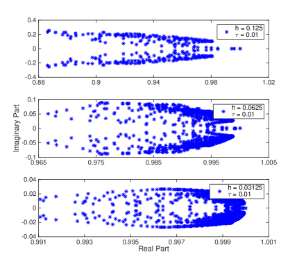
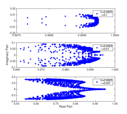
Figure 6.1: Spectrum distribution of $\displaystyle\mathcal{B}^{-1}\mathcal{A}$ when varying $\displaystyle h$ (left) and $\displaystyle\tau$ (right)

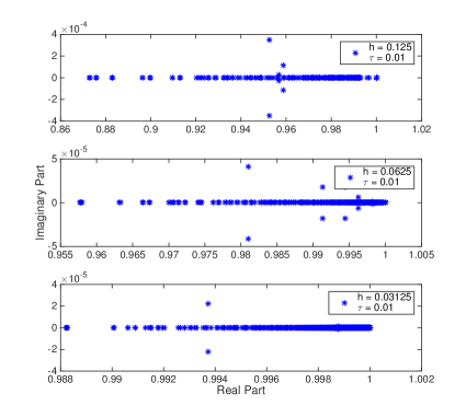
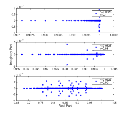
Figure 6.2: Spectrum distribution of $\displaystyle\tilde{\mathcal{B}}^{-1}\mathcal{A}$ when varying $\displaystyle h$ (left) and $\displaystyle\tau$ (right)

7 Conclusions

In this work, we propose mass lumping preconditioners for use with GMRes method to solve a class of two-by-two block linear systems which correspond to some discrete fourth order parabolic equations. Using consistent matrix in the discretization has the advantage of better solution accuracy as compared with applying mass lumping directly in the discretization. We propose to use lumped-mass matrix $\displaystyle\bar{M}$ and optimal multigrid algorithm with either coupled or decoupled smoother to construct practical preconditioners which are shown to be computationally very efficient. Numerical experiments indicate that preconditioned GMRes method converges uniformly with respect to both $\displaystyle h$ and $\displaystyle\tau$ and is robust for problems with degenerate diffusion coefficient. We provide theoretical analysis about the spectrum bound of the preconditioned system and estimate the convergence rate of the preconditioned GMRes method.

Acknowledgements

B. Zheng would like to acknowledge the support by NSF grant DMS-0807811 and a Laboratory Directed Research and Development (LDRD) Program from Pacific Northwest National Laboratory. L.P. Chen was supported by the National Natural Science Foundation of China under Grant No. 11501473. L. Chen was supported by NSF grant DMS-1418934 and in part by NIH grant P50GM76516. R. H. Nochetto was supported by NSF under Grants DMS-1109325 and DMS-1411808. J. Xu was supported by NSF grant DMS-1522615 and in part by US Department of Energy Grant DE-SC0014400. Computations were performed using the computational resources of Pacific Northwest National Laboratory (PNNL) Institutional Computing cluster systems. The PNNL is operated by Battelle for the US Department of Energy under Contract DE-AC05-76RL01830.

References

- [1] R. J. Asaro and W. A. Tiller. Interface morphology development during stress corrosion cracking: Part I. Via surface diffusion. Metallurgical Transactions, 3(7):1789–1796, 1972.
- [2] O. Axelsson, P. Boyanova, M. Kronbichler, M. Neytcheva, and X. Wu. Numerical and computational efficiency of solvers for two-phase problems. Computers Mathematics with Applications, 65(3):301–314, 2013.
- [3] O. Axelsson and M. Neytcheva. Operator splitting for solving nonlinear, coupled multiphysics problems with application to numerical solution of an interface problem. TR2011-009 Institute for Information Technology, Uppsala University, 2011.
- [4] Z.-Z. Bai, M. Benzi, F. Chen, and Z.-Q. Wang. Preconditioned MHSS iteration methods for a class of block two-by-two linear systems with applications to distributed control problems. IMA Journal of Numerical Analysis, 33(1):343–369, 2013.
- [5] Z.-Z. Bai, F. Chen, and Z.-Q. Wang. Additive block diagonal preconditioning for block two-by-two linear systems of skew-Hamiltonian coefficient matrices. Numerical Algorithms, 62(4):655–675, 2013.
- [6] Z.-Z. Bai, G. H. Golub, and M. K. Ng. Hermitian and skew-hermitian splitting methods for non-Hermitian positive definite linear systems. SIAM Journal on Matrix Analysis and Applications, 24(3):603–626, 2003.
- [7] L. Baňas and R. Nürnberg. A multigrid method for the Cahn–Hilliard equation with obstacle potential. Applied Mathematics and Computation, 213(2):290–303, 2009.
- [8] E. Bänsch, P. Morin, and R.H. Nochetto. Surface diffusion of graphs: variational formulation, error analysis, and simulation. SIAM Journal on Numerical Analysis, 42(2):773–799, 2004.
- [9] E. Bänsch, P. Morin, and R.H. Nochetto. A finite element method for surface diffusion: the parametric case. Journal of Computational Physics, 203(1):321–343, 2005.
- [10] E. Bänsch, P. Morin, and R.H. Nochetto. Preconditioning a class of fourth order problems by operator splitting. Numerische Mathematik, 118(2):197–228, 2011.
- [11] J.W. Barrett, J.F. Blowey, and H. Garcke. Finite element approximation of the Cahn–Hilliard equation with degenerate mobility. SIAM Journal on Numerical Analysis, 37(1):286–318, 1999.
- [12] M. Benzi and G. H. Golub. A preconditioner for generalized saddle point problems. SIAM Journal on Matrix Analysis and Applications, 26(1):20–41, 2004.
- [13] A.L. Bertozzi, S. Esedoglu, and A. Gillette. Inpainting of binary images using the Cahn–Hilliard equation. IEEE Transactions on Image Processing, 16(1):285–291, 2007.
- [14] J.F. Blowey and C.M. Elliott. The Cahn–Hilliard gradient theory for phase separation with non-smooth free energy part I: Mathematical analysis. European Journal of Applied Mathematics, 2(3):233–280, 1991.
- [15] J.F. Blowey and C.M. Elliott. The Cahn–Hilliard gradient theory for phase separation with non–smooth free energy. part II: Numerical analysis. European Journal of Applied Mathematics, 3:147–179, 1992.
- [16] J. Bosch, D. Kay, M. Stoll, and Andrew J. Wathen. Fast solvers for Cahn-Hilliard inpainting. SIAM Journal on Imaging Sciences, 7(1):67–97, 2014.
- [17] J. Bosch, M. Stoll, and P. Benner. Fast solution of Cahn–Hilliard variational inequalities using implicit time discretization and finite elements. Journal of Computational Physics, 262:38–57, 2014.
- [18] P. Boyanova, M. Do-Quang, and M. Neytcheva. Efficient preconditioners for large scale binary Cahn-Hilliard models. Computational Methods in Applied Mathematics, 12(1):1–22, 2012.
- [19] P. Boyanova and M. Neytcheva. Efficient numerical solution of discrete multi-component Cahn–Hilliard systems. Computers and Mathematics with Applications, 67(1):106–121, 2014.
- [20] A. Brandt and N. Dinar. Multi-grid solutions to elliptic flow problems. Numerical Methods for Partial Differential Equations, pages 53–147, 1979.
- [21] S.C. Brenner and R. Scott. The mathematical theory of finite element methods, volume 15. Springer, 2008.
- [22] J.W. Cahn and J.E. Hilliard. Free energy of a nonuniform system. i. interfacial free energy. The Journal of Chemical Physics, 28(2):258–267, 2004.
- [23] C.M. Chen and V. Thomée. The lumped mass finite element method for a parabolic problem. The Journal of the Australian Mathematical Society. Series B. Applied Mathematics, 26(03):329–354, 1985.
- [24] L. Chen. iFEM: An integrated finite element methods package in MATLAB. Technical Report, University of California at Irvine, 2009.
- [25] L. Chen. Multigrid methods for constrained minimization problems and application to saddle point problems. Submitted, 2014.
- [26] L. Chen. Multigrid methods for saddle point systems using constrained smoothers. Computers & Mathematics with Applications, 70(12):2854–2866, 2015.
- [27] S.M. Choo and Y.J. Lee. A discontinuous Galerkin method for the Cahn–Hilliard equation. Journal of Applied Mathematics and Computing, 18(1-2):113–126, 2005.
- [28] M.A. Christon. The influence of the mass matrix on the dispersive nature of the semi–discrete, second–order wave equation. Computer Methods in Applied Mechanics and Engineering, 173(1):147–166, 1999.
- [29] Q. Du and R.A. Nicolaides. Numerical analysis of a continuum model of phase transition. SIAM Journal on Numerical Analysis, 28(5):1310–1322, 1991.
- [30] C.M. Elliott. The Cahn–Hilliard model for the kinetics of phase separation. In Mathematical models for phase change problems, pages 35–73. Springer, 1989.
- [31] C.M. Elliott and D.A. French. Numerical studies of the Cahn–Hilliard equation for phase separation. IMA Journal of Applied Mathematics, 38(2):97–128, 1987.
- [32] C.M. Elliott and D.A. French. A nonconforming finite-element method for the two-dimensional Cahn-Hilliard equation. SIAM Journal on Numerical Analysis, 26(4):884–903, 1989.
- [33] C.M. Elliott, D.A. French, and F.A. Milner. A second order splitting method for the Cahn-Hilliard equation. Numerische Mathematik, 54(5):575–590, 1989.
- [34] C.M Elliott and S. Larsson. Error estimates with smooth and nonsmooth data for a finite element method for the Cahn–Hilliard equation. Mathematics of Computation, 58(198):603–630, 1992.
- [35] X. Feng and O. Karakashian. Fully discrete dynamic mesh discontinuous Galerkin methods for the Cahn-Hilliard equation of phase transition. Mathematics of computation, 76(259):1093–1117, 2007.
- [36] X. Feng and A. Prohl. Error analysis of a mixed finite element method for the Cahn–Hilliard equation. Numerische Mathematik, 99(1):47–84, 2004.
- [37] X. Feng and A. Prohl. Numerical analysis of the Cahn–Hilliard equation and approximation for the Hele–Shaw problem. Journal of Computational Mathematics, 26(6):767–796, 2008.
- [38] I. Fried. Bounds on the spectral and maximum norms of the finite element stiffness, flexibility and mass matrices. International Journal of Solids and Structures, 9(9):1013–1034, 1973.
- [39] D. Furihata. A stable and conservative finite difference scheme for the Cahn-Hilliard equation. Numerische Mathematik, 87(4):675–699, 2001.
- [40] F.J. Gaspar, F.J. Lisbona, C.W. Oosterlee, and R. Wienands. A systematic comparison of coupled and distributive smoothing in multigrid for the poroelasticity system. Numerical Linear Algebra with Applications, 11(2-3):93–113, 2004.
- [41] C. Gräser and R. Kornhuber. On preconditioned Uzawa-type iterations for a saddle point problem with inequality constraints. In Springer, editor, Domain Decomposition Methods in Science and Engineering XVI, volume 55 of Lect. Notes Comput. Sci. Eng., pages 91–102, Berlin, 2007.
- [42] J.B. Greer and A.L. Bertozzi. solutions of a class of fourth order nonlinear equations for image processing. Discrete and Continuous Dynamical Systems, 10(1/2):349–366, 2004.
- [43] P.M. Gresho, R.L. Lee, and R.L. Sani. Advection-dominated flows, with emphasis on the consequences of mass lumping. In Finite Elements in Fluids, volume 1, pages 335–350, 1978.
- [44] Y. He and Y. Liu. Stability and convergence of the spectral Galerkin method for the Cahn–Hilliard equation. Numerical Methods for Partial Differential Equations, 24(6):1485–1500, 2008.
- [45] S. Henn. A multigrid method for a fourth-order diffusion equation with application to image processing. SIAM Journal on Scientific Computing, 27(3):831–849, 2005.
- [46] E. Hinton, T. Rock, and O.C. Zienkiewicz. A note on mass lumping and related processes in the finite element method. Earthquake Engineering & Structural Dynamics, 4(3):245–249, 1976.
- [47] D. Kay and R. Welford. A multigrid finite element solver for the Cahn–Hilliard equation. Journal of Computational Physics, 212(1):288–304, 2006.
- [48] J. Kim, K. Kang, and J. Lowengrub. Conservative multigrid methods for Cahn–Hilliard fluids. Journal of Computational Physics, 193(2):511–543, 2004.
- [49] B.B. King, O. Stein, and M. Winkler. A fourth-order parabolic equation modeling epitaxial thin film growth. Journal of Mathematical Analysis and Applications, 286(2):459–490, 2003.
- [50] O. Lass, M. Vallejos, A. Borzi, and C.C. Douglas. Implementation and analysis of multigrid schemes with finite elements for elliptic optimal control problems. Computing, 84(1-2):27–48, 2009.
- [51] R. Mullen and T. Belytschko. Dispersion analysis of finite element semidiscretizations of the two-dimensional wave equation. International Journal for Numerical Methods in Engineering, 18(1):11–29, 1982.
- [52] D.A. Niclasen and H.M. Blackburn. A comparison of mass lumping techniques for the two-dimensional Navier-Stokes equations.pdf. In Twelfth Australasian Fluid Mechanics Conference, pages 731–734. The Univesity of Sydney, 1995.
- [53] M.A. Olshanskii and A. Reusken. Navier–Stokes equations in rotation form: a robust multigrid solver for the velocity problem. SIAM Journal on Scientific Computing, 23(5):1683–1706, 2002.
- [54] A. Quarteroni. On mixed methods for fourth–order problems. Computer Methods in Applied Mechanics and Engineering, 24(1):13–34, 1980.
- [55] J. Schöberl. Multigrid methods for a parameter dependent problem in primal variables. Numerische Mathematik, 84:97–119, 1999.
- [56] Z. Sun. A second-order accurate linearized difference scheme for the two-dimensional Cahn-Hilliard equation. Mathematics of Computation, 64(212):1463–1471, 1995.
- [57] S. Takacs and W. Zulehner. Convergence analysis of multigrid methods with collective point smoothers for optimal control problems. Computing and Visualization in Science, 14(3):131–141, 2011.
- [58] L.N. Trefethen and M. Embree. Spectra and pseudospectra: The behavior of nonnormal matrices and operators. Princeton Univeristy Press, 2005.
- [59] T. Ushijima. On the uniform convergence for the lumped mass approximation of the heat equation. Journal of the Faculty of Science, University of Tokyo, 24:477–490, 1977.
- [60] T. Ushijima. Error estimates for the lumped mass approximation of the heat equation. Memoirs Numerical Mathematics, 6:65–82, 1979.
- [61] S.P. Vanka. Block-implicit multigrid solution of Navier-Stokes equations in primitive variables. Journal of Computational Physics, 65:138–158, 1986.
- [62] M. Wang and L. Chen. Multigrid methods for the stokes equations using distributive Gauss–Seidel relaxations based on the least squares commutator. Journal of Scientific Computing, 56(2):409–431, 2013.
- [63] S. Wise, J. Kim, and J. Lowengrub. Solving the regularized, strongly anisotropic Cahn–Hilliard equation by an adaptive nonlinear multigrid method. Journal of Computational Physics, 226(1):414–446, 2007.
- [64] G. Wittum. Multigrid methods for Stokes and Navier–Stokes eqautions with transforming smoothers: algorithms and numerical results. Numerische Mathematik, 54(5):543–563, 1989.
- [65] Y. Xia, Y. Xu, and C.W. Shu. Local discontinuous Galerkin methods for the Cahn–Hilliard type equations. Journal of Computational Physics, 227(1):472–491, 2007.
- [66] X. Ye and X. Cheng. The Fourier spectral method for the Cahn–Hilliard equations. Numerische Mathematik, 171(1):545–357, 2005.
- [67] S. Zhang and M. Wang. A nonconforming finite element method for the Cahn–Hilliard equation. Journal of Computational Physics, 229(19):7361–7372, 2010.