A status update on the determination of $\Lambda_{\overline{\rm MS}}^{N_{\rm f}=3}$
by the ALPHA collaboration

Abstract:

The ALPHA collaboration aims to determine $\alpha_{s}(m_{Z})$ with a total error below the percent level. A further step towards this goal can be taken by combining results from the recent simulations of $2+1$-flavour QCD by the CLS initiative with a number of tools developed over the years: renormalized couplings in finite volume schemes, recursive finite size techniques, two-loop renormalized perturbation theory and the (improved) gradient flow on the lattice. We sketch the strategy, which involves both the standard SF coupling in the high energy regime and a gradient flow coupling at low energies. This implies the need for matching both schemes at an intermediate switching scale, $L_{\rm swi}$, which we choose roughly in the range 2-4 ${\rm GeV}$. In this contribution we present a preliminary result for this matching procedure, and we then focus on our almost final results for the scale evolution of the SF coupling from $L_{\rm swi}$ towards the perturbative regime, where we extract the $N_{\rm f}=3$ $\Lambda$-parameter, $\Lambda_{\overline{\rm MS}}^{(3)}$, in units of $L_{\rm swi}$. Connecting $L_{\rm swi}$ and thus the $\Lambda$-parameter to a hadronic scale such as $F_{K}$ requires 2 further ingredients: first, the connection of $L_{\rm swi}$ to $L_{\rm max}$ using a few steps with the step-scaling function of the gradient flow coupling, and, second, the continuum extrapolation of $L_{\rm max}F_{K}$.

TCDMATH 15–11
DESY 15-218
CERN-PH-TH-2015-269
WUB/15-08
HU-EP-15/54
IFT-UAM/CSIC-15-122

1 Introduction

One of the long-term goals of the ALPHA-collaboration consists in a controlled and precise determination of the strong coupling constant, $\alpha_{s}$, from experimentally well-measured hadronic observables. In 2+1-flavour QCD the hadronic input can be obtained using gauge field ensembles produced by Coordinated Lattice Simulations (CLS) effort [1, 2]. The 3 bare parameters, $m_{u}=m_{d}$, $m_{s}$ and the coupling $g_{0}$ can be fixed taking e.g. $m_{\pi}$, $m_{K}$ and $F_{K}$ from experiment, after correcting for isospin breaking and electromagnetic effects. Once this is achieved, any other observable of the theory becomes a prediction, in particular, the renormalized strong coupling at a large scale,

$$\alpha_{s}^{(N_{\rm f}=3)}(1000\times F_{K}),\qquad\alpha_{s}=\dfrac{\bar{g}^{2}}{4\pi},$$ (1)

in any renormalization scheme. Obviously the final goal is to determine $\alpha_{s}^{(N_{\rm f}=5)}(m_{Z})$ in the $\overline{\rm MS}$-scheme of dimensional regularization. This requires a matching procedure to $4$- and $5$-flavour QCD across the charm and bottom thresholds, respectively. There is some hope that perturbation theory may be adequate to include not only the effects of the heavier bottom quark on the coupling, but also those of the charm quark [3, 4]. This will not be discussed here. We just mention that current phenomenological estimates of $\alpha_{s}$ yield

$$\alpha_{s}(m_{Z})=0.1183(12)\,,$$ (2)

with a 1% error [5]. This is compatible with the currently available lattice results which have total errors of similar size [6]. Using the strategy described in the following we expect a significant reduction of this error.

2 The $\Lambda$-parameter and $\alpha_{s}$

Given the strong coupling $\alpha_{s}=\bar{g}^{2}/(4\pi)$ in a quark mass independent renormalization scheme the corresponding $\Lambda$-parameter is defined by

$$\Lambda^{(N_{\rm f})}=\mu\big{[}b_{0}\bar{g}^{2}(\mu)\big{]}^{-b_{1}/(2b_{0}^{2})}\,{\rm e}^{-1/(2b_{0}\bar{g}^{2}(\mu))}\exp\bigg{\{}\!\!-\!\!\int_{0}^{\bar{g}^{\vphantom{A}}(\mu)}\!dg\bigg{[}\dfrac{1}{\beta(g)}+\dfrac{1}{b_{0}g^{3}}-\dfrac{b_{1}}{b_{0}^{2}g}\bigg{]}\bigg{\}},$$ (3)

where $N_{\rm f}$ denotes the fixed number of quark flavours. If the coupling constant is non-perturbatively defined, so is the $\beta$-function and thus the $\Lambda$-parameter. Nevertheless, at high scales the perturbative form $\beta(g)=-b_{0}g^{3}-b_{1}g^{5}+\ldots$ can be used, with the universal coefficients,

$$b_{0}=\dfrac{11-\frac{2}{3}N_{\rm f}}{(4\pi)^{2}},\qquad b_{1}=\dfrac{102-\frac{38}{3}N_{\rm f}}{(4\pi)^{4}}\,.$$ (4)

The relation between the $\Lambda$-parameters in any two schemes is exactly calculable by one-loop perturbation theory: for schemes ${\rm X}$ and ${\rm Y}$ the one-loop relation between the respective couplings entails the relation,

$$g_{\rm X}^{2}=g_{\rm Y}^{2}+c_{\rm XY}g_{\rm Y}^{4}+{\rm O}(g_{\rm Y}^{6})\quad\Rightarrow\quad\dfrac{\Lambda_{\rm X}}{\Lambda_{\rm Y}}={\rm e}^{c_{\rm XY}/2b_{0}}\,.$$ (5)

Hence, even though the $\overline{\rm MS}$-scheme is only defined perturbatively, its $\Lambda$-parameter can be defined non-perturatively and is conventionally used as a reference. Note that a 1% error on $\alpha_{s}(m_{Z})$ translates to a 6-7% error on $\Lambda^{(5)}_{\overline{\rm MS}}$ [5], which sets the reference in terms of the precision.

3 An approach involving 2 couplings

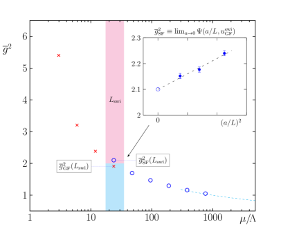
The approach to compute $\Lambda^{(3)}_{\overline{\rm MS}}$ followed by our collaboration has previously been described in ref. [7] and is sketched in fig. 1. Moving up the energy scale from the hadronic to the perturbative regimes it consists of the four separate steps:

1. Matching of a hadronic scale, e.g. $F_{K}$, to the box size $L_{\rm max}$ defined implicitly through the gradient flow coupling of ref. [8], $\bar{g}^{2}_{\rm GF}(L_{\rm max})=u_{\rm max}$. Here the value $u_{\rm max}$ must be chosen such that there is a range of common values of $\beta=6/g_{0}^{2}$, so that the limit

   $$\lim_{a\rightarrow 0}\left(aF_{K}\right)(\beta)\times\left(L_{\rm max}/a\right)(\beta)\,,$$ (6)

   can be taken. As the matching proceeds via the bare parameters the same lattice action must be used as in the CLS simulations.

2. As a next step we calculate the evolution of the GF coupling from $L_{\rm max}$ to an intermeditate scale, $L_{\rm swi}=2^{-3}L_{\rm max}$, by 3 steps up the energy scale by factors of 2. One may do a step more or less, and the scale factor need not be 2 in all the steps. In fact, $L_{\rm swi}$ can be defined in a variety of ways. The only thing that matters is that the relation between $L_{\rm max}$ (and thus $F_{K}$) and a given choice of $L_{\rm swi}$ is known precisely.

3. At the intermediate scale $L_{\rm swi}$ we switch scheme to the traditional SF coupling [9, 10], $\bar{g}^{2}_{\rm SF}(L_{\rm swi})$. At this point we also change the gauge action to the Wilson plaquette action.

4. The evolution of the SF coupling is traced by doing 3-5 steps up the energy scale with scale factor 2. At small couplings the $\Lambda$-parameter can then be extracted in units of $L_{\rm swi}$ using a perturbative evaluation of the exponent in eq. (3).

Figure 1: A sketch of the strategy (cp. text), reproduced from ref. [7].

We use 2 different couplings and gauge actions for technical reasons: first, the target precision for the $\Lambda$-parameter from eq. (3) requires the knowledge of the 3-loop $\beta$-function, which is only available for the SF coupling [11]. Furthermore, cutoff effects in the SF coupling have been calculated to 2-loop order with the Wilson gauge action and their subtraction from the data, helps to stabilise the continuum limit. Finally the scaling properties of the statistical errors at fixed $L/a$ with the scale $L$ favour the SF coupling towards the perturbative high energy regime [7]. Combining the advantages of both couplings seems the best strategy, the price to pay being the additional scheme switching step.

4 Computation of $L_{\rm swi}\Lambda$

Figure 2: Left panel: The data points interpolated to common $u$-values, together with the global fit function, The rightmost points were not included in the fit. Right panel: The continuum extrapolated SSF with its error band (shaded area) together with the data points (cp. text).

The scale evolution of the SF coupling $\bar{g}^{2}(L)$ can be traced by constructing the step-scaling function (SSF)

$$\sigma(u)=\left.\bar{g}^{2}(2L)\right|_{\bar{g}^{2}(L)=u},$$ (7)

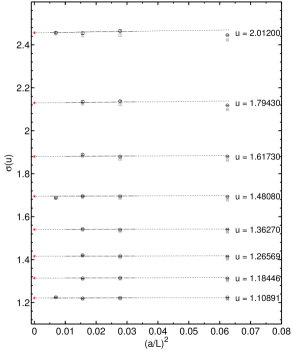
as the continuum limit of lattice approximants, $\Sigma(u,a/L)$. This requires to compute the SF coupling on pairs of lattices $L/a$ and $2L/a$ at the same bare parameters. We have measured $\Sigma(u,L/a)$ for lattice sizes $L/a=4,6,8$ and in 3 cases for $L/a=12$, and for 6 approximately tuned $u$-values in the interval $[1.08,2.012]$. The critical mass has been tuned to high precision so that the corresponding systematic effects are completely negligible. Furthermore, the knowledge of perturbation theory to 2-loop order allows to subtract the cutoff effects completely at a given perturbative order: with

$$\delta(u,a/L)=\dfrac{\Sigma(u,a/L)}{\sigma(u)}-1=\delta_{1}(L/a)\times u+\delta_{2}(L/a)\times u^{2}+{\rm O}(u^{3}),$$ (8)

we may define the 2-loop perturbatively improved data,

$$\widetilde{\Sigma}(u,a/L)=\dfrac{\Sigma(u,a/L)}{1+\delta_{1}(L/a)u+\delta_{2}(L/a)u^{2}}\,.$$ (9)

Given the data points we perform global fits to both the perturbatively improved and unimproved data. An example for such a fit ansatz is

$$\widetilde{\Sigma}(u,a/L)=u+s_{0}u^{2}+s_{1}u^{3}+c_{1}u^{4}+c_{2}u^{5}+\rho_{1}\dfrac{a^{2}}{L^{2}}u^{4},$$ (10)

which we apply to all the data with $L/a\geq 6$. Here,

$$s_{0}=2b_{0}\ln 2,\qquad s_{1}=s_{0}^{2}+2b_{1}\ln 2,$$ (11)

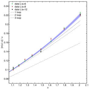
are fixed to their perturbative values, the fit parameters $c_{1}$ and $c_{2}$ describe the continuum SSF and $\rho_{1}$ models the cutoff effects. The main assumption of such a global fit ansatz is the smoothness of both the continuum SSF and the cutoff effects as a function of $u$. With 19 data points and 3 parameters the fit in eq. (10) has a reasonable $\chi^{2}/{\rm d.o.f.}=1.0$. 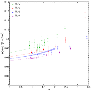The data points, slightly interpolated to common values of $u$, are displayed together with the resulting continuum SSF in figure 2. A comparison with data from the literature for $N_{\rm f}=0$ [12], $N_{\rm f}=2$ [13, 14], $N_{\rm f}=3$ [15] and $N_{\rm f}=4$ [16] is made in figure 3.

Figure 3: Comparison with results from the literature for $N_{\rm f}=0,2,3,4$ [12, 13, 14, 15, 16]. The shaded area corresponds to the global fit. The dashed lines show the perturbative prediction $b_{0}+{\rm O}(u)$.

We now define the switching scale, $L_{\rm swi}$, through the SF coupling by setting,

$$\bar{g}^{2}_{\rm SF}(L_{\rm swi})=2.012,$$ (12)

which is the largest $u$-value for which we have computed the SSF. Taking this value as our starting point, we may now recursively step up the energy scale by factors of 2, using the fitted continnum SSF, viz.

$$u_{0}=\bar{g}^{2}_{\rm SF}(L_{\rm swi}),\quad u_{i}=\sigma(u_{i+1}),$$ (13)

where $i=0,1,2,\ldots$. Then, using the formula for the $\Lambda$-parameter, eq. (3) and its relation to $\Lambda_{\overline{\rm MS}}$ [10],

$$\Lambda_{\rm SF}^{(3)}=0.38286(2)\times\Lambda_{\overline{\rm MS}}^{(3)}\,,$$ (14)

we obtain stable results already after a couple of steps. As our preliminary result we quote

$$L_{\rm swi}\Lambda_{\overline{\rm MS}}^{(3)}=0.0802(24)\,,$$ (15)

with a total error of 3 percent.

5 Matching to the GF coupling

Having finished step 4 of our strategy, we now discuss step 3, the matching to the gradient flow coupling. We define the GF coupling in a finite volume with SF boundary conditions following [8]. However, in order to reduce boundary effects, we restrict the sum to the chromo-magnetic components by summing over spatial Lorentz indices only,

$$-\frac{1}{2}\sum_{k,l=1}^{3}t^{2}\left.\langle G_{kl}(t,x)G_{kl}(t,x)\rangle\right|_{x_{0}=T/2,T=L,t=c^{2}L^{2}/8,m_{\rm q}=0}={\cal N}(c,a/L)\times\bar{g}_{\rm GF}^{2}(L)\,.$$ (16)

We use both the Wilson flow [17, 18] and the O($a^{2}$) improved Zeuthen flow [19, 20] and an O($a^{2}$) improved definition of the observable [19, 21]. For the matching we employ the Wilson plaquette action, whereas the scale evolution (step 2 of the strategy) will use the Lüscher-Weisz gauge action to match the set-up of CLS.

Figure 4: Matching the GF and SF couplings using the line of constant physics $\bar{g}_{\rm SF}^{2}(L_{\rm swi})=2.012$ (cp. text).

We note that $c$ defines the smoothing range in units of $T=L$. Staying in the middle of the volume, $x_{0}=T/2$ and setting $c=0.3$ we expect that the influence from the time boundaries is negligible. This is further corroborated by a perturbative analysis. Then, using the $\beta$- and $\kappa$-values that correspond to the line of constant physics (LCP) condition $\bar{g}^{2}(L_{\rm swi})=2.012$, for $L/a=6,12,16$ we double the lattice size, switch off the background field and thus obtain the (preliminary) results in figure 4. As our preliminary continuum extrapolation we quote,

$$\bar{g}_{\rm GF}^{2}(2L_{\rm swi})=2.680(10)\,.$$ (17)

This illustrates the typical precision that can be obtained: note that this error includes an estimate of the uncertainty in the definition of the LCP (hence the 2 kinds of error bars in fig. 4). We also mention that the cutoff effects are naturally expressed in units of the smoothing radius, $a/\sqrt{8t}=a/(cL)$, which is the reason for doubling the lattice size as compared to the SF coupling.

6 Summary

We have presented our preliminary result $\Lambda_{\overline{\rm MS}}^{(3)}=0.0802(24)/L_{\rm swi}$, where $L_{\rm swi}$ is an intermediate scale, defined implicitly by $\bar{g}_{\rm SF}^{2}(L_{\rm swi})=2.012$. Furthermore, we have matched the SF and GF couplings with the (preliminary) result $\bar{g}_{\rm GF}^{2}(2L_{\rm swi})=2.680(10)$. To finish the project, it remains to relate $L_{\rm swi}$ to a hadronic scale by computing the SSF for the GF coupling towards lower enery scales, and by matching the maximal box size, $L_{\rm max}$, reached in this way to a hadronic scale such as $F_{K}$, as measured on the CLS gauge configurations.

Acknowledgments

This project is part of the ALPHA collaboration research programme. We would like to thank the computer centres at HLRN and NIC at DESY-Zeuthen for providing computing resources. S. Sint acknowledges support by SFI under grant 11/RFP/PHY3218.

References

- [1] M. Bruno et al., JHEP 1502, 043 (2015) [arXiv:1411.3982 [hep-lat]].
- [2] talk by S. Schaefer at this conference.
- [3] M. Bruno et al. [ALPHA Collaboration], Phys. Rev. Lett. 114, no. 10, 102001 (2015) [arXiv:1410.8374 [hep-lat]].
- [4] A. G. Grozin, M. Hoeschele, J. Hoff, M. Steinhauser, JHEP 1109, 066 (2011) [arXiv:1107.5970 [hep-ph]].
- [5] Particle Data Group, J. Beringer et al., Phys.Rev. D86 (2012) 010001, and 2013 partial update for the 2014 edition.
- [6] S. Aoki et al., Eur.Phys.J. C74 (2014) 2890, 1310.8555.
- [7] P. Fritzsch et al. [ALPHA Collaboration], PoS LATTICE 2014 (2014) 291 [arXiv:1411.7648 [hep-lat]].
- [8] P. Fritzsch and A. Ramos, JHEP 1310, 008 (2013) [arXiv:1301.4388 [hep-lat]].
- [9] M. Lüscher et al., Nucl.Phys. B384 (1992) 168, hep-lat/9207009.
- [10] S. Sint and R. Sommer, Nucl. Phys. B 465, 71 (1996) [hep-lat/9508012].
- [11] A. Bode, P. Weisz and U. Wolff [ALPHA Collaboration], Nucl.Phys. B576 (2000) 517, hep-lat/9911018, [Erratum-ibid. B 600 (2001) 453], [Erratum-ibid. B 608 (2001) 481].
- [12] M. Lüscher et al., Nucl.Phys. B413 (1994) 481, hep-lat/9309005.
- [13] M. Della Morte et al. [ALPHA Collaboration], Nucl.Phys. B713 (2005) 378, hep-lat/0411025.
- [14] P. Fritzsch et al., Nucl. Phys. B 865, 397 (2012) [arXiv:1205.5380 [hep-lat]].
- [15] S. Aoki et al. [PACS-CS Collaboration], JHEP 0910, 053 (2009) [arXiv:0906.3906 [hep-lat]].
- [16] F. Tekin, R. Sommer and U. Wolff [ALPHA Collaboration], Nucl.Phys. B840 (2010) 114, 1006.0672.
- [17] R. Narayanan and H. Neuberger, JHEP 0603 (2006) 064, hep-th/0601210.
- [18] M. Lüscher, JHEP 1008 (2010) 071, 1006.4518.
- [19] A. Ramos and S. Sint, arXiv:1508.05552 [hep-lat].
- [20] A. Ramos and S. Sint, PoS LATTICE 2014, 329 (2015) [arXiv:1411.6706 [hep-lat]].
- [21] Z. Fodor et al., JHEP 1409, 018 (2014) [arXiv:1406.0827 [hep-lat]].