Helicity inversion in spherical convection as a means for equatorward dynamo wave propagation
Abstract
We discuss here a purely hydrodynamical mechanism to invert the sign of the kinetic helicity, which plays a key role in determining the direction of propagation of cyclical magnetism in most models of dynamo action by rotating convection. Such propagation provides a prominent, and puzzling constraint on dynamo models. In the Sun, active regions emerge first at mid-latitudes, then appear nearer the equator over the course of a cycle, but most previous global-scale dynamo simulations have exhibited poleward propagation (if they were cyclical at all). Here, we highlight some simulations in which the direction of propagation of dynamo waves is altered primarily by an inversion of the kinetic helicity throughout much of the interior, rather than by changes in the differential rotation. This tends to occur in cases with a low Prandtl number and internal heating, in regions where the local density gradient is relatively small. We analyse how this inversion arises, and contrast it to the case of convection that is either highly columnar (i.e., rapidly rotating) or locally very stratified; in both of those situations, the typical profile of kinetic helicity (negative throughout most of the northern hemisphere) instead prevails.
keywords:
convection – dynamo – hydrodynamics – magnetic fields – turbulence – Sun: general – stars: general1 Introduction
The systematic equatorward migration of sunspot emergence latitudes constitutes one of the most enduring puzzles of solar physics. Spots appear first at mid-latitudes, then progressively nearer the equator over the course of a roughly 11-year cycle (e.g., Carrington 1858; Maunder 1904; reviews in Ossendrijver 2003, Hathaway & Rightmire 2010), constituting the famous “butterfly diagram". There is now widespread agreement that the surface magnetism ultimately arises from the action of a dynamo within the Sun’s electrically conducting convection zone, but a detailed explanation for the equatorward propagation has remained elusive (see, e.g., Moffatt, 1978). In many models of the global solar dynamo, this propagation is taken to reflect underlying wave-like behaviour in the generation of sub-surface magnetism (see, e.g., review in Charbonneau, 2010; Priest, 2014).
In the classic model developed by Parker (1955) and explored by many other authors since (e.g., Yoshimura, 1975; Stix, 1976; Gilman, 1983), the wave-like behaviour arises from the combination of helical turbulence and differential rotation, described in mean-field theory by the -effect and -effect, respectively (e.g., Steenbeck et al. 1966; review in Brandenburg & Subramanian 2005). The former encapsulates the production of poloidal magnetic field from toroidal (or vice versa) by convective eddies that rise and twist, while the latter describes the generation of toroidal field by linear winding of a poloidal field by differential rotation. In an dynamo, the sign of newly generated toroidal field is determined by the sense of the differential rotation and by the sign of the pre-existing poloidal field. The latter in turn depends on the properties of the convective flows. The direction of propagation of the dynamo wave is then determined by the locations where toroidal field, generated by the differential rotation from stretching of poloidal field loops, cancels or enhances the pre-existing toroidal field: if the newly generated field tends preferentially to cancel pre-existing field near the equator and reinforce it at higher latitudes, the migration of the field will be poleward. This is encapsulated by the well-known Parker-Yoshimura sign rule that dynamo waves in such models travel in a direction given by (Yoshimura, 1975; Stix, 1976).
The sign of the -effect, which partly determines the direction of propagation of the dynamo wave, is fundamentally related to the lack of reflectional symmetry in the flow: changes sign under transformations from right-handed to left-handed coordinate systems, and vanishes if the velocity field is statistically invariant under such parity transformations (see, e.g., Moffatt, 1978). In many variants of mean field theory, assuming certain simplifying features about the velocity field, can in turn be related to the kinetic helicity of the flow, (with the vorticity), often in addition to other terms involving the current helicity (e.g., Pouquet et al., 1976; Brandenburg & Subramanian, 2005). The sign and spatial variation of the kinetic helicity are thus crucial for determining the direction of field propagation.
In the past few decades, a wide variety of published nonlinear dynamo simulations in spherical geometries have been shown to exhibit cyclical behaviour (e.g., Gilman 1983; Ghizaru et al. 2010, in the context of stellar astrophysics, or Goudard & Dormy 2008; Schrinner et al. 2011; Simitev & Busse 2012; Gastine et al.; 2012 in the planetary context). However, to the extent that these simulations have exhibited systematic latitudinal propagation, this has generally been poleward (see, e.g., discussion in Brun et al., 2013), in agreement with the Parker-Yoshimura rule (given the realized kinetic helicity and differential rotation) but in conflict with the observed solar butterfly diagram. More recently, a few groups have published examples of convective dynamos whose propagation is equatorward: e.g., Käpylä et al. (2012, 2013); Augustson et al. (2013); Warnecke et al. (2014). In each of these cases, the equatorward migration has been attributed largely to features in the differential rotation: e.g., to regions where the radial gradient is negative (Käpylä et al., 2012; Warnecke et al., 2014), or to non-linear feedbacks on the shear (Augustson et al., 2015). The kinetic helicity profile in these simulations, and with it the purported -effect, appears to be largely as described in Sec. 2.1 below, and as realized in many previous simulations: it is negative in the northern hemisphere, leading to a positive -effect.
In this paper, we explore the circumstances under which the kinetic helicity, and with it the generation of poloidal magnetic fields, actually has this spatial distribution. In Sec. 2 we review the processes that lead to this helicity distribution, and outline a scenario in which it could instead have the opposite sign throughout much of the spherical domain. In Sec. 3, we carry out non-linear simulations of anelastic convective dynamos in global spherical shells, and show that these can indeed exhibit such “reversed" kinetic helicity profiles in certain regimes. We demonstrate that simulations exhibiting this reversal also show systematic equatorward propagation of dynamo waves, without any accompanying changes in the differential rotation. We analyse the mechanisms behind the kinetic helicity reversal more thoroughly in Sec. 4, and close in Sec. 5 with a summary of our work and a discussion of its possible relevance to the Sun, other stars, and planets.
2 Regimes of kinetic helicity
2.1 Classical helicity configuration in global dynamo simulations
The kinetic helicity , calculated as
| (1) |
arises from the twisting and writhing of convective flows as they rise or fall. It is instructive to consider two regimes of convection that have been the subject of particularly wide study, which we will call “columnar" and “plume-like". The former has been widely studied in the planetary context (see, for example Busse, 1970; Busse & Cuong, 1977; Olson et al., 1999; Busse, 2002; Aubert, 2005; Aubert et al., 2008) and found to dominate in rapidly-rotating systems at lower Rossby numbers. In Boussinesq models, the transition to such behaviour has been discussed by Soderlund et al. (2012) and we will address this matter in Sec. 5.2.
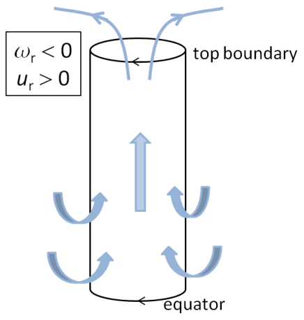
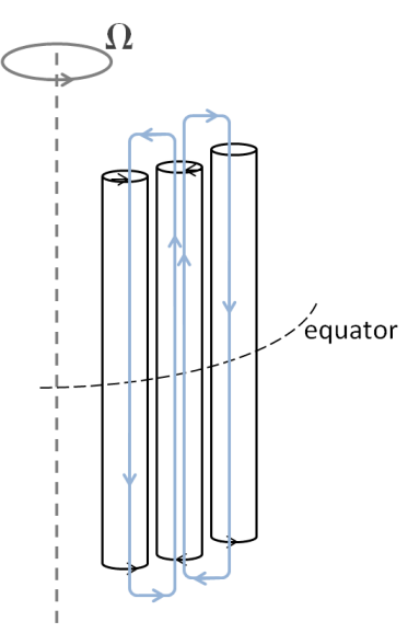
Columnar convection consists of dominating nearly 2D (quasi-geostrophic) circular motions (i.e. independent of the cylindrical coordinate, defined by the rotation axis) with a secondary axial flow induced mainly by the boundaries along the columns for a Boussinesq fluid (Busse et al., 1998; Olson et al., 1999). The 2D vortical motion arises from diverging up flow encountering the top and bottom boundaries, generating clockwise vortical motion. Since the resulting radial vorticity from the diverging up flow is negative in the North hemisphere and positive in the Southern (as a result of the Coriolis force acting on it), the component of the resulting vorticity is negative in both hemispheres. The flow will then sink toward the equatorial plane and converge to start rising again, generating now counter-clockwise motion (positive , see Olson et al., 1999, and also Fig. 1). While the divergence of the flow occurs mainly near the boundaries, convergence can happen anywhere in the bulk and not exclusively at the equator (Fig. 1). According to the Taylor-Proudman constraint (Proudman, 1916; Taylor, 1922), the local axes of vorticity tend to align with the rotation axis , shaping columns of alternating vorticity sign. As illustrated in Fig. 2, is positive in the northern hemisphere and negative in the southern along columns with positive and vice-versa. This means that in columnar convection, the kinetic helicity is dominated by the cylindrical component in . Thus will always be negative in the northern hemisphere ( and have opposite sign) and positive in the southern ( and have the same sign). This helicity organization is helpful to obtain a large scale dipole field (e.g Olson et al., 1999). Note that columnar convection is also present in some plane-layer models (Childress & Soward 1972 and an example of application in numerical models, Stellmach & Hansen 2004), thus it does not necessarily depend on the spherical geometry.
A second regime, in which stratification and buoyancy instead play central roles, also often results in a similar kinetic helicity profile. In this “plume-like" regime, more akin to the classic Rayleigh-Bénard convection problem, convection consists of rising and sinking flow between the inner and outer boundaries, predominantly along the radial direction. We generally expect that this type of convection will replace columnar convection in a rotating system when the effect of rotation is weak compared to buoyancy.
This regime is easily attained near the surface of strongly stratified models of stellar and planetary convection (see, e.g., Miesch et al. 2008; Glatzmaier et al. 2009; Gastine et al. 2013; review in Miesch & Toomre 2009), where the density gradient is much steeper leading to comparatively larger Rossby numbers (ratio between inertia and Coriolis force, e.g. Browning, 2008; Gastine & Wicht, 2012; Gastine et al., 2013). Furthermore, a higher value of Rossby number may also intensify helicity (see Sec. 4.1 below). According to the anelastic continuity equation,
| (2) |
when the density gradient is dominant (second term on the right side), a parcel rising along expands due to the rapidly decreasing density toward the surface (Fig. 4). The Coriolis force acts on the expanding fluid to generate anticyclonic fluid motion (negative in the northern hemisphere and positive in the southern, see Glatzmaier, 1985). In addition, the rising velocity decreases as a fluid parcel slows down when approaching the outer boundary, which may also decrease the effect of the incompressible term of the continuity equation (first term on the right side). For the same reason, sinking flow contracts generating cyclones (positive in the northern hemisphere and negative in the southern). Both effects of the rising/sinking flow naturally correlate as negative helicity, so plume-like convection near the surface typically gives a hemispherical North/South helicity pattern similar to that of columnar convection. Both types of convection often co-exist and reinforce each other in stratified models.
2.2 “Inverted" helicity configuration
In the previous section, we described the most commonly observed case of helicity distribution in numerical dynamo models in rotating spherical shells. In the presence of milder density stratification () and rapid rotation, convection is often dominated by columnar convection. If on the other hand buoyancy dominates and the medium is highly stratified, plume-like convection (consisting of expanding upflows and contracting downflows) often prevails. Both lead to a kinetic helicity profile that is predominantly negative in the northern hemisphere. But what happens under other circumstances?
In the presence of a weak density contrast, roughly , a rising fluid parcel will tend to contract since its velocity is increasing as it starts from the bottom with (impenetrable boundaries). More generally, this may be true even far from the boundaries if . This is easily understood from the equation of mass conservation (Eq. 2) when assuming that is small. Such small density contrasts typically exist in stratified models in the inner of the radius (see Sec. 3 below, particularly Fig. 4). Consequently, the continuity equation becomes approximately the Boussinesq continuity equation of in the deeper part of the shell. Figure 3 illustrates schematically this behaviour below the dashed line which is a representation of the inner part of the radius of a spherical shell. In this region, the density gradient is relatively smaller than above the dashed line, which represents the outer few percent where typically most of the density gradient is located.
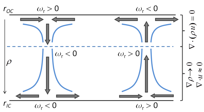
In the region of small density gradient below the dashed line of Fig. 3, the Coriolis force acts on the rising+contracting fluid generating positive radial vorticity in the northern hemisphere and negative in the southern (cyclones). In the same region in the same way, sinking flow expands as it slows down toward the bottom boundary, generating anticyclones. In both cases of rising+contracting and sinking+expanding flows, the resulting sign of helicity is positive in the northern hemisphere and negative in the southern. This behaviour is opposite to the outer layer (described in the previous Section) and it seems only pertinent when columnar convection becomes minimal in the bulk.
In this schematic picture, explored in more detail in the following Sections, the inversion of kinetic helicity is a purely hydrodynamical effect, independent of the magnetic field, though it will ultimately be important to determine the direction of the poloidal field generated by the -effect and consequently the sign of the generated toroidal field, which explains the direction of propagation of a dynamo wave in the Parker-model.
It is also useful to distinguish between the possibility of deep layers where the kinetic helicity is “reversed" (i.e., positive in the northern hemisphere), as explored here, from well-known boundary effects that would tend to lead to the same profile within a narrow layer close to the bottom of the convection zone. It has long been anticipated that such reversals of kinetic helicity would arise at the base of the solar convection zone, for example, where convective downflows begin to be buoyantly braked and spread (e.g., Brummell et al., 2002). But in simple parametrizations of the solar dynamo, the layer where this reversal is achieved is typically taken to be confined to a region near the bottom of the convective envelope or below its base (e.g., Charbonneau, 2010). The convergence of flows to feed plumes that are beginning to rise buoyantly from a bottom thermal boundary layer is also well known (Julien et al., 1996; Nishikawa & Kusano, 2002; Dubé & Charbonneau, 2013; Guervilly et al., 2014) and is likewise somewhat distinct from the distributed helicity profiles described here, though the same basic physical mechanisms underlie all these. This will be demonstrated in the following Sections.
3 Model
3.1 Numerical model
For this work, we used the code MagIC111https://github.com/magic-sph/magic to solve an anelastic version of the MHD equations, following Gilman & Glatzmaier (1981), Braginsky & Roberts (1995) and Lantz & Fan (1999), in a rotating spherical shell. This code implements a dimensionless formulation, where the length scale is the shell thickness , the time is non-dimensionalized by the viscous time (where is the kinematic viscosity) and the temperature, gravity and density by their values at the outer boundary, respectively , and . Lastly, the magnetic field unit is given by , where is the rotation rate, the magnetic permeability and the magnetic diffusivity at the bottom boundary of the domain, . The dimensionless equations are
| (3) |
| (4) |
| (5) |
| (6) |
| (7) |
where , and are the velocity, magnetic field and entropy fields, respectively, is the aspect ratio given by and the traceless rate-of-strain tensor S for homogeneous is
| (8) |
and is the identity matrix. The viscous and ohmic heating contributions are
| (9) |
and
| (10) |
The background reference state is defined by the temperature gradient and the background density is derived as , where the tilde corresponds to the background reference state and is the polytropic index. The dissipation number is expressed as
| (11) |
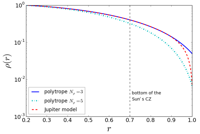
where is the number of density scale heights and and are the radii of the inner and outer boundaries, respectively. In Fig. 4, the solid blue line corresponds to and and the cyan dot-dashed line to and . The red dashed line corresponds to a polynomial fit of Jupiter’s interior model (French et al., 2012), where the corresponding was obtained from the best corresponding to the data for the background temperature from the same model. The result is and .
Finally, the control parameters in Eqs. (3–7) correspond to ratios between pairs of terms of the Navier-Stokes equation, namely the Ekman number (viscous over Coriolis force), the Rayleigh number (measure of the convective driving of the system) and the fluid and magnetic Prandtl numbers,
| (12) |
| (13) |
| (14) |
where , and are the thermal, viscous and magnetic diffusivities, respectively. In our models, we fixed and we used and for the ratios between diffusivities. The Rayleigh number is either entropy-based or flux-based as follows
| (15) |
where if the boundary conditions of the energy equation are fixed entropy and for the models where the boundaries are assumed fixed flux. The quantities and are the specific entropy flux at the outer boundary and the specific heat capacity at constant pressure, respectively.
Even though the results discussed in this paper were first found in our Jupiter models with variable magnetic diffusivity (as reported by Jones, 2014), we simplified some of these models by carrying out a small number of hydrodynamic and magnetic simulations with constant transport properties along radius, to illustrate our conclusions. The variable conductivity profile used in the Jupiter models is described in Gastine et al. (2014).
3.2 Numerical method
The MagIC code uses a pseudo-spectral method to solve the MHD equations described above. Spherical harmonics are used in the horizontal direction () up to degree and order and Chebyshev polynomials in the radial direction up to degree (see Wicht, 2002, for a more detailed description). The equations are solved in the commonly used poloidal/toroidal decomposition of the divergence-free fields and (Eqs. 6 and 7) as
| (16) |
where and are the poloidal potentials of and , respectively, while and are the toroidal counterparts. The radial unit vector is represented by .
The boundary conditions applied in our simulations are the same for the velocity and magnetic fields. Following previous work which had the purpose of modelling the gas giants (Gastine & Wicht, 2012; Gastine et al., 2012; Duarte et al., 2013), the inner boundary is assumed no-slip and the inner core is modelled as an electrical conductor. Top boundary is considered free-slip and the magnetic field is there matched to a potential field. The entropy boundary conditions and heating modes vary in our models. Several of our cases assume simple bottom heating, i.e. the entropy contrast between the bottom and top boundaries is fixed and there is no internal heating in the system, thus the heating entering the system through the bottom boundary exits through the top. The other two set-ups for the energy equation considered here account for internal heat sources: in one case with fixed entropy boundaries and in the other with fixed flux boundary conditions.
3.3 Diagnostic parameters
In the following Sections we will describe the flow by often referring to several dimensionless diagnostic parameters to be consistent with the formulation outlined in the previous Sections.
The amplitude of the flow contributions is measured in terms of the Rossby numbers . The value of is calculated as
| (17) |
where is the rms volume-averaged flow velocity and the triangular brackets denote the angular average
| (18) |
The local Rossby number has been introduced by Christensen & Aubert (2006) to quantify the relative importance of the advection term in the Navier-Stokes equation (Eq. 3). Here we consider only the non-axisymmetric part of the flow velocity (i.e. velocity excluding the axisymmetric flow component) to calculate the local convective Rossby number, defined as
| (19) |
where, is a typical flow length scale given by
| (20) |
Here is the flow contribution of spherical harmonic degree .
The geometry of the surface field is characterized by the dipolarity
| (21) |
which measures the relative energy in the axial dipole contribution at the outer boundary .
Finally, to describe the behaviour of the various components of the flow, we used correlations between pairs of variables. A correlation between two sets of data and in the form of 3D matrices corresponding to the three spherical coordinates is calculated at each radial level as
| (22) |
The parameters described in this Section are listed along control parameters in Tab. LABEL:TabRes, averaged over at least viscous time. The values of the Rayleigh number necessary for the onset of convection as defined by Jones et al. (2009) (i.e., where all other dimensionless control parameters are fixed), were obtained for cases without internal heating. These values were used to obtain the supercriticality values listed in Tab. LABEL:TabRes at constant Ekman number. In the same table, simulations without internal heating correspond to (see Eq. 5) and if internal heating is present. Concerning the entropy boundary conditions corresponding to columns (bottom) and (top), values and indicate fixed entropy and flux, respectively.
4 Kinetic helicity realized in non-linear simulations
4.1 Numerical hydro/dynamo models
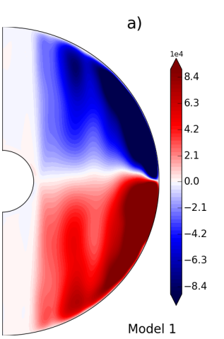
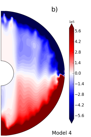
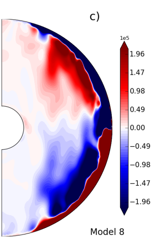

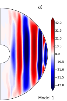
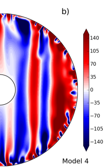
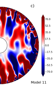
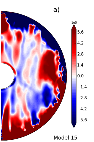
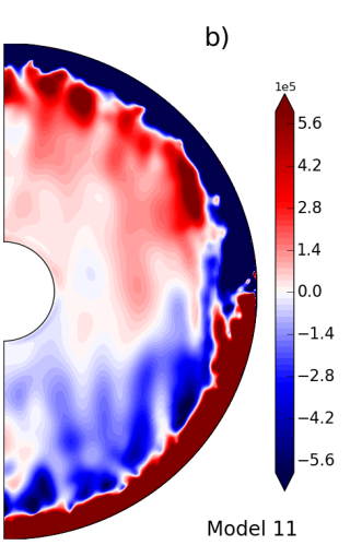
Figure 5 illustrates the two helicity configurations described in Secs. 2.1 and Sec. 2.2 for global hydrodynamical and dynamo simulations in a rotating spherical shell, for two different supercriticalities. Contour plots of azimuthally-averaged kinetic helicity are shown here for snapshots, since these helicity patterns are not time-dependent in our models. The top panels show the usual one-layer negative(North)/positive(South) helicity configuration for the combination of columnar convection and plume-like convection from Sec. 2.1. The bottom plots show the two-layer behaviour described in Sec. 2.2 and illustrated in Fig. 3. In each row, the supercriticality of the models increases from left to right, hence the later onset of convection inside the tangent cylinder TC (cylinder tangent to the inner core boundary around the rotation axis) on the left-side panels. As mentioned in the Introduction, the different sign of helicity (e.g. top and bottom rows of Figure 5) is obtained for models which retain similar differential rotation profiles, as shown in Figure 6. As evident in Fig. 6, the differential rotation is solar-like in the sense of having a faster equator. Model 4 does however exhibit some non-geostrophic flow that breaks the equatorial symmetry (Gastine et al., 2012). This Figure also shows an additional model (case of Tab. LABEL:TabRes) because we refer to that simulation later in Sec. 4.2.
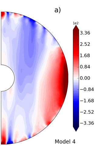
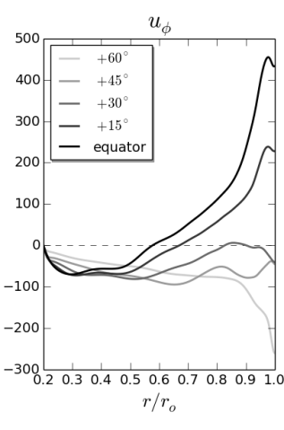
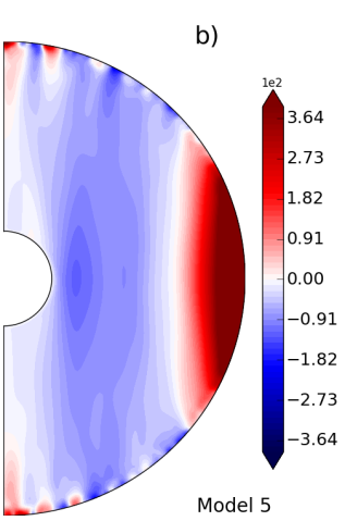
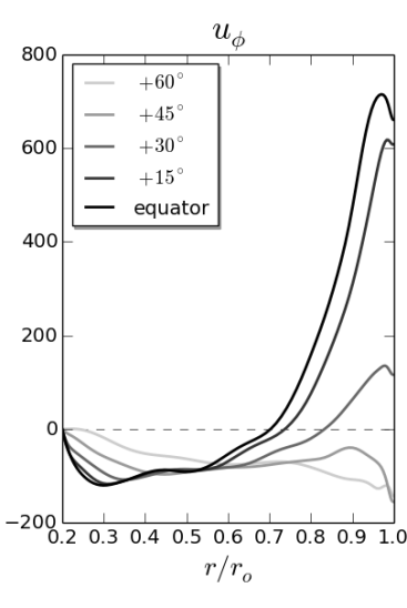
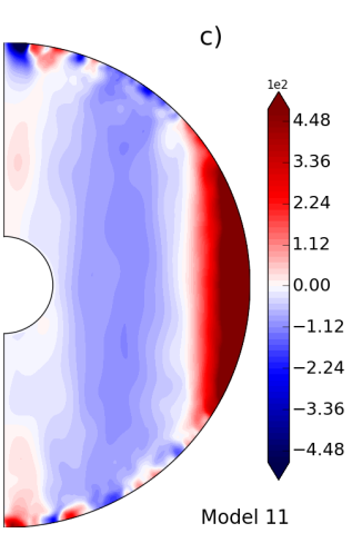
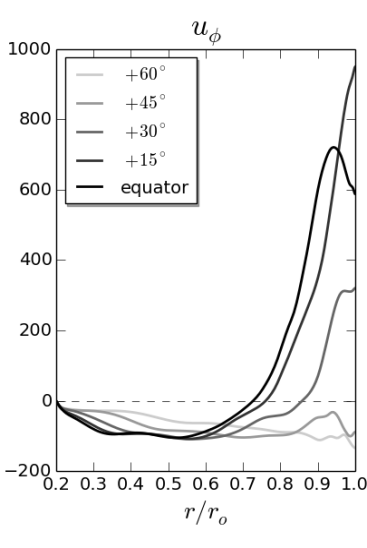
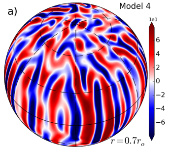
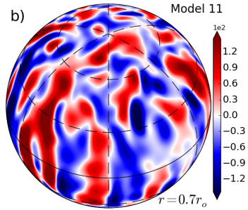
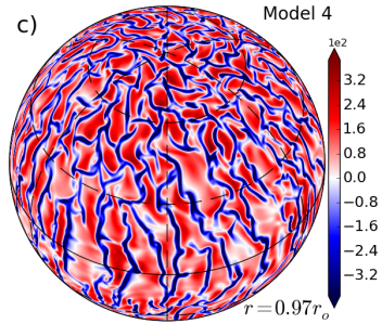
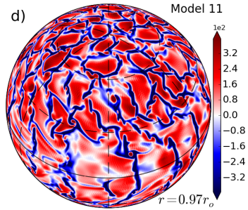
Figure 7 shows radial velocity contour plots for three cases displayed in Fig. 5, namely the top row and the right panel of the bottom row. Figure 8 displays models and in orthographic projection to illustrate the latitudinal/longitudinal distribution of the flow features at the two depths described in Secs. 2.1 and 2.2. The leftmost panel of Fig. 7 (and top left panel of 5) is distinctly dominated by columnar convection. The middle panel has a stronger density gradient in the outer part of the shell as Fig. 4 shows, resulting in a break down of the columns in the outer radius, where convection becomes dominated by radial features (see Fig. 12 of Gastine et al., 2013). Below this outer layer, convection remains under a columnar regime, though combined with plume-like convection. This set-up corresponds to the one-layer helicity pattern described in Sec. 2.1, where both types of convection co-exist in strongly stratified models. The right panel corresponds to the two-layer helicity pattern described in Sec. 2.2, where convection is seemingly not columnar any more. In this case, the density gradient used was the interior model for Jupiter in Fig 4, which may help achieving this configuration since, even though the density contrast is also around 5 density scale heights, it now concentrates most of the gradient in the outer of the radius of the shell. However, this is not the only difference, as we will discuss next.
Perhaps more significantly, the cases in Figs. 5–8 that show “inverted" helicity (models and ) also differ from the other cases displayed here in these Figures by adopting a lower value of and a different mode of heating. While in the top row panels of Fig. 5, as in most of our previous work (for example, Gastine & Wicht, 2012; Gastine et al., 2012; Yadav et al., 2013; Duarte et al., 2013), the cases in the bottom row have a lower value of . The effect of lowering the Prandtl number has been thoroughly studied by Simitev & Busse (2005); Sreenivasan & Jones (2006), where their main conclusion was the significant increase of the role of inertia when decreasing by one order of magnitude or more from unity. When inertia enters the force balance at a significant degree, the columnar convection constraint weakens in the bulk, as discussed by Christensen & Aubert (2006). The change of heating mode in conjunction with fixed flux boundaries is also crucial. An internal heating source has been shown to spread convection in the domain, thus also weakening convection in the bulk as it tends to detach the deeper convective motions from the inner boundary (Hori et al., 2010). With fixed entropy boundary conditions, on the other hand, changes in the internal heating mode did not appear to change the outcome in our simulations (see however Jones, 2014, for a possible counter-example).
Lowering the value of appears to be the most important factor in changing the helicity pattern due to its relation to the amount of inertia in the system, with a tendency to promote plume-like convection. When applying only a different heating mode or a different density profile or both, we saw very little difference in the final results of our models as the one-layer helicity configuration remains dominant. However, lowering alone is not sufficient either. In Fig. 9, we show two cases with the same lower Prandtl number , though convection in the left panel is driven by bottom heating and on right by internal heating proportional to the background density profile (Eq. 5). The left panel shows that indeed the inversion to attain the helicity regime of Sec. 2.2 is not complete unless we combine the lower with internal heating.
In conclusion, the combination of the three effects (high , low and internal heating) is important to achieve the required degree of non-columnar/plume-like convection in the bulk of the shell. The requirement of high is harder to constrain and appears to be inconsistent with the requirement for negligible density contrast in the interior. This apparent contradiction is because the higher the overall density contrast, the closer we get to a negligible density gradient in the bulk. Even though this does not eliminate the possibility of Sec. 2.2 also occurring in a weakly stratified or even Boussinesq model, cases and in Tab. LABEL:TabRes show a helicity pattern very similar to the plane layer configuration, with a symmetry about half of the height (Julien et al., 1996), or half the radius in the case of a spherical shell. How exactly this symmetry about the mid-plane is broken by the combination of density stratification and internal heating, and whether the “inverted" helicity layers studied here require both these elements or are conceptually unrelated, requires further study.
Käpylä et al. (2013) has reported a relation between the rotation rate and the degree of stratification for the onset of oscillatory solutions, which we did not explore here: they find that at higher , lower is necessary to find oscillatory solutions. They also argued that equatorward wave solutions occur only at larger , whereas poleward propagation is found instead at milder density contrasts.
4.2 Dynamo waves
In Fig. 10 we show a few examples of butterfly diagrams constructed from our models, to illustrate the consequence of the different helicity patterns described above, in rough accordance with the Parker model. The top left panel shows a previous simulation from our previous Jupiter models which has a poleward-propagating dynamo wave for comparison (see Gastine et al., 2012; Duarte et al., 2013). The other three panels exemplify the variety of equatorward propagating waves found in the models described here. In some cases, the equatorward part is confined to a lower latitudinal band with weak poleward propagation at high latitudes, likely due to the lack of convection inside the TC at lower supercriticality (see examples of Fig. 5). Nonetheless, this higher-latitude feature is common in most models and a similar higher latitude feature has also been observed in the Sun (Hathaway & Upton, 2014).
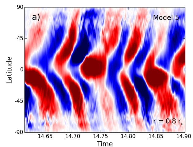
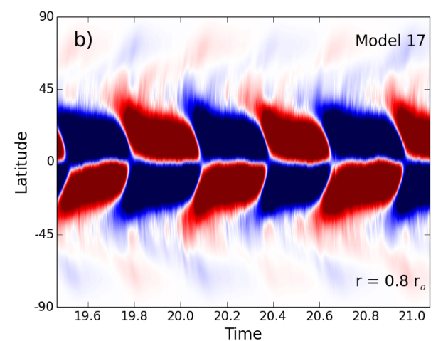
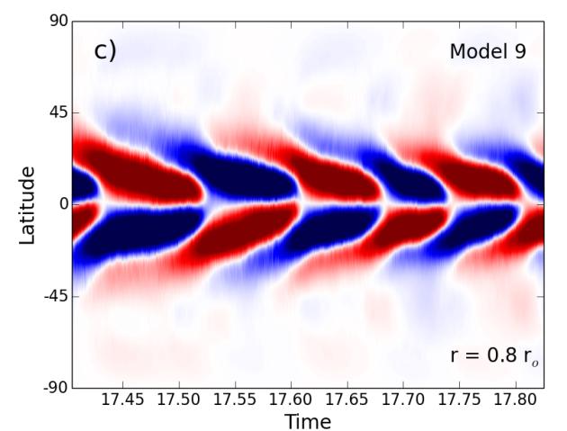
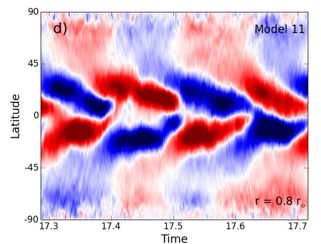
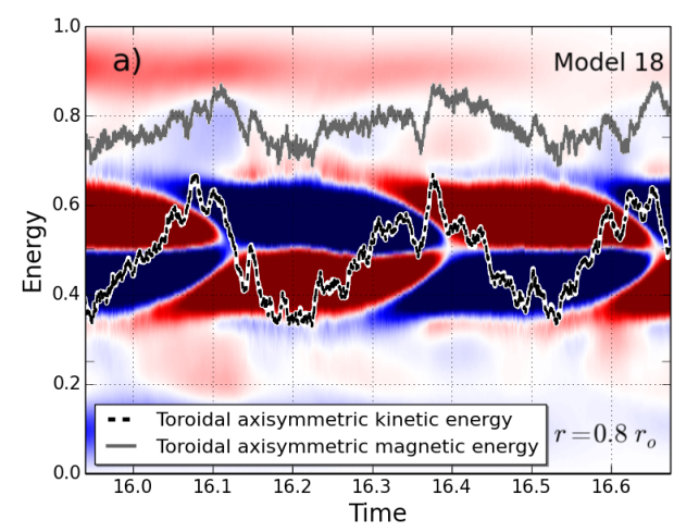
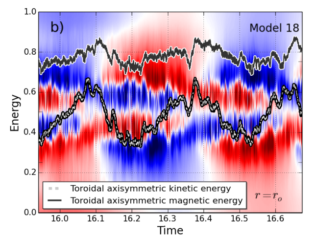
Figure 11 shows two butterfly diagrams for the same model. The toroidal field is shown on the left panel at the same depth as in Fig. 10 and the poloidal field is shown at the surface in the right panel. These two panels demonstrate that the wave-like motion is also observed at the surface of our models, which would result in a Sun-like butterfly diagram. Following Gilman (1983), we also plotted here the axisymmetric toroidal components of the kinetic (dashed line) and magnetic (solid line) energies, normalized by the total kinetic and magnetic energies, respectively. As Gilman (1983) reported, it is possible to identify the imprint of the wave in the kinetic and magnetic energy time series.
A detailed study of dynamo cases is out of the scope of this paper, since we intended to focus simply on the mechanisms that alter the kinetic helicity and with it the direction of migration. Aspects related to the magnetic field will be further analysed in future work. For some of these cases, the dynamo wave is not stable, eventually stabilizing in an octupolar solution, which may be related to the use of variable transport properties from our work on Jupiter models.
5 Analysis and interpretation
5.1 Correlations to describe flow behaviour
According to the idealized scenario described in Sec. 2.1, columnar convection often dominates in the inner part of the shell, where the ‘rising/sinking’ component of the flow (along a column and away from the equator) is anti-symmetric about the equator but (since the column rotates in the same direction in both hemispheres) is symmetric. Converting between cylindrical and spherical coordinate systems,
| (23) |
where represents here the cylindrical radius, we see that the radial component of the velocity is symmetric over the equator, while is anti-symmetric. The radial quantities are particularly relevant in strongly stratified models, where convection becomes plume-like thus the preferred ’rising/sinking’ direction is along spherical radius. At each radial level, divergence and convergence of the flow is represented by the horizontal divergence of the flow (in spherical coordinates)
| (24) |
A similar divergence can be adapted to columnar convection, by assuming a horizontal plane defined by the cylindrical coordinates at a fixed height , thus replacing by and similarly by .
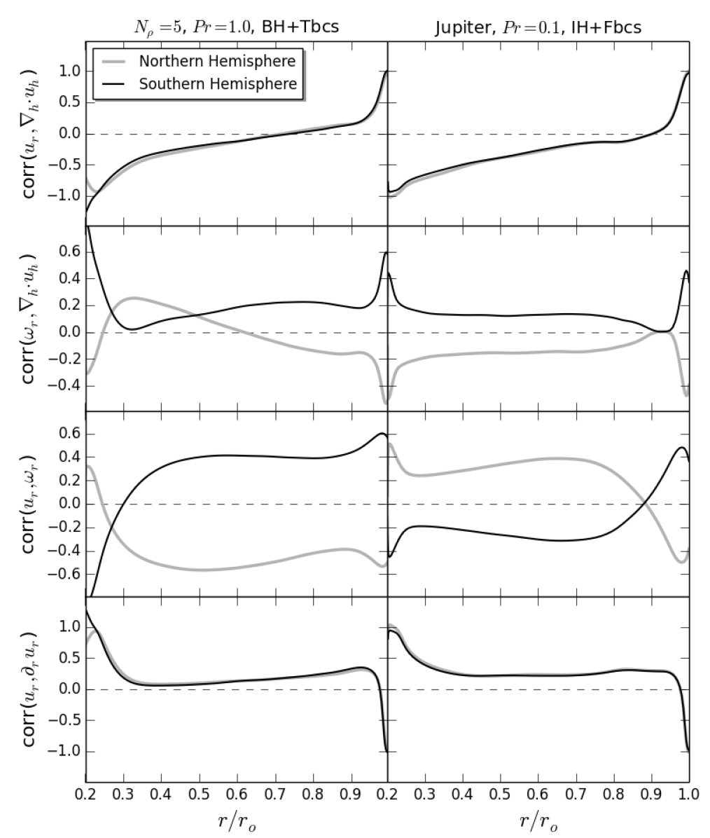
Figure. 12 shows several correlations between different properties of the rising/sinking flow that dominate convection, only in the radial direction for a first analysis. The model of the panels of the left column represents the helicity set-up described in Sec. 2.1 and the model of the right column corresponds to the set-up described in Sec. 2.2. Focusing mainly on the right column, since we expect convection to be non-columnar here, in the top panel we see that the rising velocity correlates negatively with the horizontal divergence throughout most of the radius as expected, i.e. as the flow rises it contracts and when it sinks it diverges, as described in Sec. 2.2. The picture naturally inverts in the outer of the layer, where the density gradient dominates, causing a positive correlation between the two quantities. The second-row panel on the right side shows the expected role of the Coriolis force acting on the diverging/converging flow to generate negative/positive in the northern hemisphere (grey line) and positive/negative in the southern (black line). The third panel correlates directly and , clearly showing that rising/sinking flow in the outer of the shell gives negative/positive vorticity, while the picture inverts in the bulk. This panel also translates directly into the preferred sign of kinetic helicity, negative near the surface but positive below (Sec. 2.2 scenario). Finally, the bottom panel displays the correlation between and the acceleration or deceleration of the fluid, since in the continuity equation it is that is ultimately linked to horizontal divergence/convergence (if the compressible term is negligible). This shows that the flow is consistently speeding up as it rises as well as slowing down when it sinks in most of the shell, which explains the tendency to contract as it rises.
The left column of Fig. 12 displays a model which has been shown in the previous Section to be mostly dominated by columnar convection in the bulk, resulting in the helicity pattern described in Sec. 2.1. As a result, the radial correlations displayed in the left column of Fig. 12 show some inconsistencies and asymmetries between the two hemispheres, while the right side panels of the same Figure show almost perfect symmetry. This occurs because in columnar convection, such quantities are better expressed in terms of the cylindrical coordinate. Thus Fig. 12 shows two examples of changes in the flow regime as the rotational constraint is varied, as also seen in the values of convective local Rossby number: and for the models on the left and right columns, respectively.
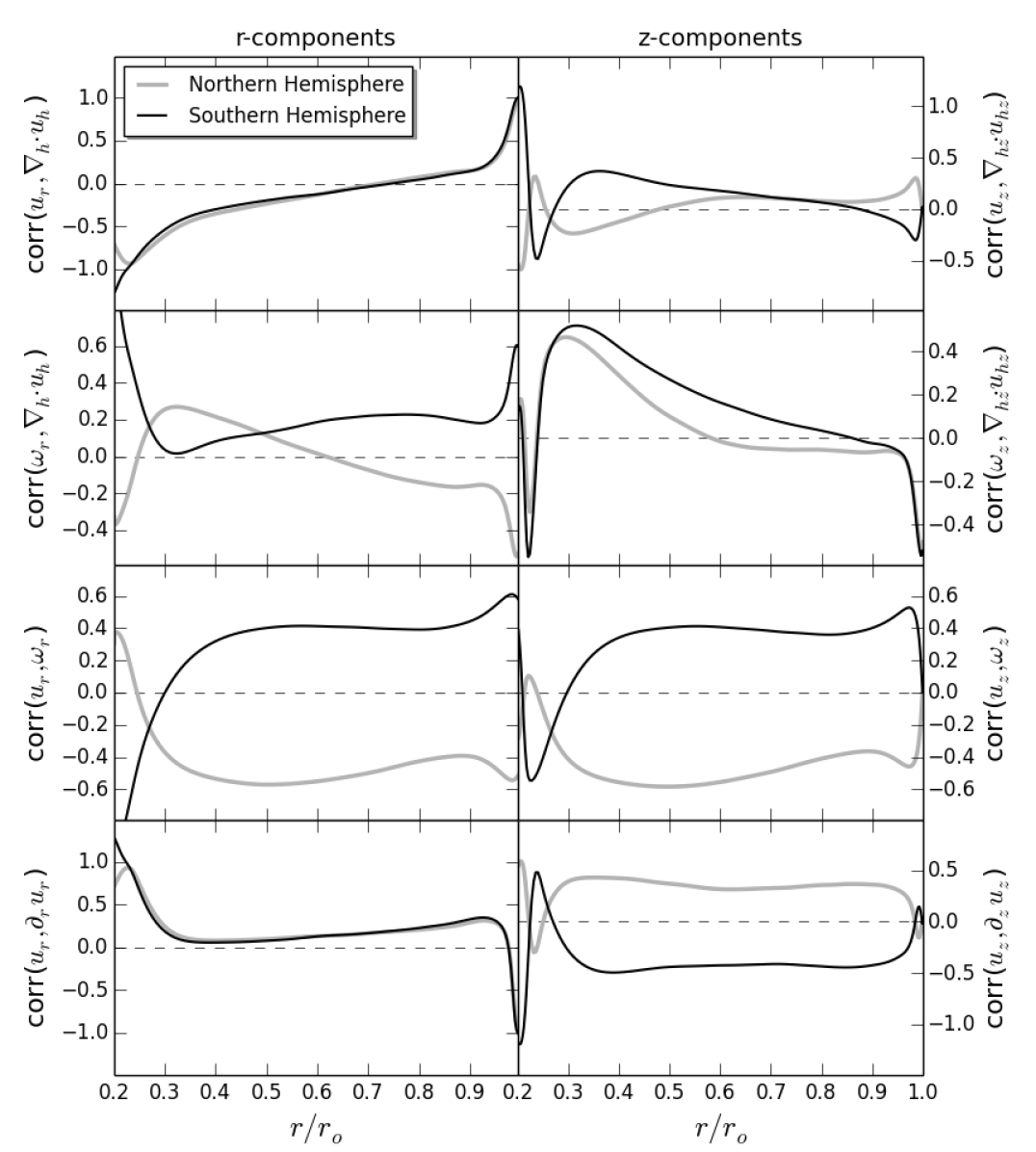
Figure 13 shows the same left column of Fig. 12 and the right column represents equivalent calculations for the same model along , as described in the beginning of this Section. There is some asymmetry in both columns, since there is a small superposition of the two convective regimes, but the right column more clearly illustrates the behaviour of the flow. In the right top panel, when is positive (away from the equator and toward the upper boundary) in the northern hemisphere, the flow will diverge at the top of a column which is seen by tracking the grey line. The inner part is an exception though, likely due to either a superposition with the radial component or to the influence of convection inside the TC (not explored here) since the correlations shown are averaged over horizontal spherical coordinates (see caption of Fig. 12). An asymmetry is also perceptible in the second row, though the cylindrical coordinate system plays the major role in contributing the positive peak near the bottom of the layer () in the radial correlations between and in the northern hemisphere (grey line). As illustrated above in Fig. 1, the flow diverges mainly at the extremities of a column with negative , where it encounters the bottom and top boundaries, but it converges along its length in most of the bulk. This explains the positive peak of in the bottom half of the shell that directly affects the sign of through Eq. 23, appearing to result in an inconsistent behaviour of the Coriolis force in the radial component. It’s the cylindrical calculation on the right panel of the second row that is most relevant for this part of the shell. The top four panels show this persistent asymmetry between the two hemispheres as a direct consequence of the different symmetries between / and /. This asymmetry is also seen in the bottom four panels, though more camouflaged. In particular the third row once again shows the clear resulting sign of kinetic helicity in the majority of the shell, consistent with the set-up described in Sec. 2.1.
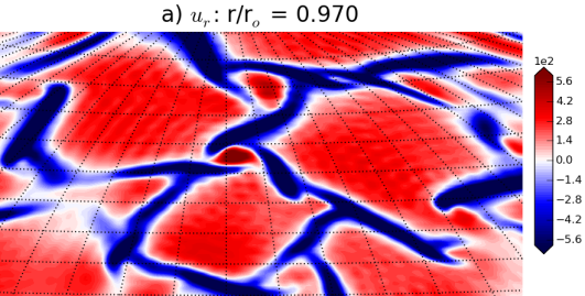
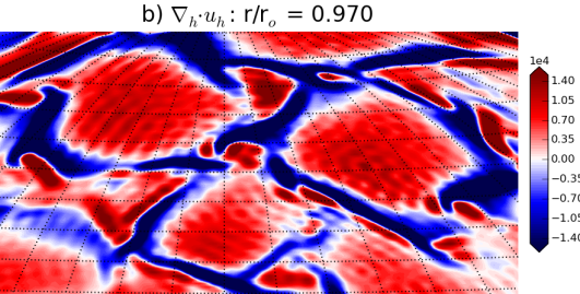
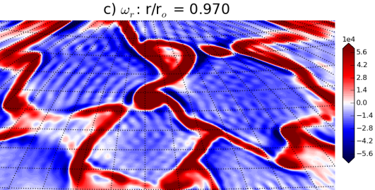
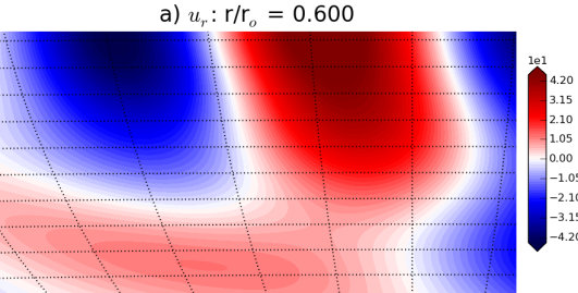
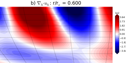
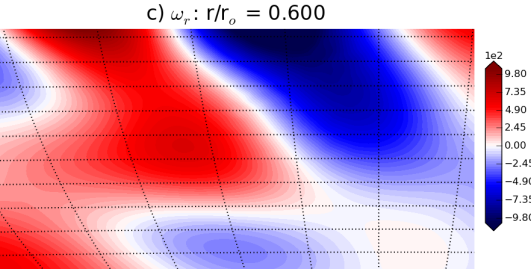
Figure 14 shows a segment of the near-surface maps of different properties of the flow to illustrate the typical behaviour of the flows at the outer radii common for most strongly stratified models. In the northern hemisphere, the flow rises (first panel from the top), expands as the density decreases (horizontal divergence of the horizontal velocity , in the third panel) and rotates clockwise (negative in the second panel, i.e. anti-cyclones – see Sec. 2.1). The same happens when the flow sinks as it is promptly compressed in the filaments seen in these three panels around the sources represented by the horizontal divergence of the horizontal flow .
Figure 15 illustrates the alternative convection mechanism in the inner part of the shell described in Sec. 2.2, at a depth of below the surface of the model. The different dynamics shown above in Fig. 12 by the inversion of sign in the correlations of the third row, can also be seen here as positive in the top panel of Fig. 15 now correlates with negative horizontal divergence (middle panel) and thus negative (cyclones, see Sec. 2.2) due to the action of the Coriolis force. However, these linkages are less clear than in Figure 14, or the idealised description of Sec. 2.2, partly because of the complexity of the flow field and because a variety of processes contribute at some level to vorticity generation. On average, though, as Fig. 12 shows, upflows in this region are well correlated with horizontally convergent flows.
5.2 Columnarity
Contour plots of radial velocity shown in Fig. 7 of the previous Section show the predominance of the columnar convection regime in the bulk of a spherical shell, as suggested in Sec. 2.2. Near the surface both set-ups of Secs. 2.1 and 2.2 are identical, except for a slight difference in the scale of the convection, since lower value of is known to produce larger convective flow scales (Jones et al., 2009). At deeper radial levels as discussed above, columnar convection tends to remain the dominant type of convection, while still predominantly plume-like near the surface. Soderlund et al. (2012) defined a parameter they called “Columnarity", meant to determine the degree at which the flow is organized in convection columns. They defined this parameter from the ratio of the integral of in the cylindrical -direction and the integral in of the total RMS vorticity of the flow:
| (25) |
where primes mean that vorticity is calculated from the non-axisymmetric part of the velocity field.
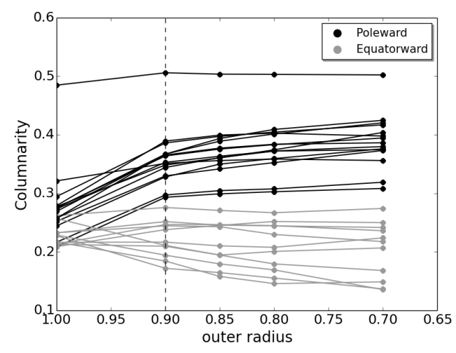
This parameter works well for Boussinesq models, where convection onsets and remains attached to the inner boundary, unless the supercriticality is large enough (typically above 50-100 times supercritical). We saw that even though this criterion works fairly well for mildly stratified models (e.g. ), it is not descriptive enough for strongly stratified models. However, the previous Sections suggest that the most likely reason for this is that even though the flow is still columnar in the bulk, it is not in the outer of the radius. This will naturally affect the total value of since the integration includes this outer part of the shell where convection is not columnar. As a result, the value of is nearly the same for models with different helicity patterns. We attempted to calculate below deeper radii to remove the major effect of the outer part and thus find a way to still use this parameter to distinguish one-layer helicity models from two-layer. The result is shown in Fig. 16 for several of our models, obtained from snapshots. By excluding the outer part, it appears indeed possible to separate the two regimes using , i.e. to separate the poleward-propagating wave models from the equatorward ones. The two different rotational regimes represented by the grey/black lines are also characterized by a generally higher value of , as mentioned in previous Section.
6 Discussion and application to stars
In many classic theories of stellar and planetary dynamos, the direction of propagation of dynamo “waves" is determined partly by the differential rotation and partly by the kinetic helicity (e.g., Parker, 1955; Steenbeck et al., 1966; Moffatt, 1978). In broad accordance with this expectation, many prior dynamo simulations that possessed some form of cyclical behavior have exhibited poleward propagation of fields (Gilman, 1983; Ghizaru et al., 2010; Goudard & Dormy, 2008; Schrinner et al., 2011; Simitev & Busse, 2012; Gastine et al., 2012; Duarte et al., 2013), in keeping with the realized profiles of helicity and differential rotation but in contrast to what is seen in the Sun. Notable exceptions in the stellar context include Käpylä et al. (2013); Augustson et al. (2013), and Warnecke et al. (2014), who attributed equatorward propagation in the simulations primarily to changes in the differential rotation profile. In those simulations, as in prior ones exhibiting poleward propagation, the kinetic helicity of the flows appears to have remained predominantly negative in the northern hemisphere (positive in the southern hemisphere), in accord with theoretical expectations for both columnar and highly stratified convection (as summarized in Sec. 2.1). In the planetary context, models with equatorward propagating dynamo waves in a set-up closer to ours were reported by Jones (2014) for “failed" Jupiter-like simulations, carried out at lower values of Prandtl number and always driven by internal heating.
We have examined here whether the kinetic helicity in global-scale convection simulations of stars and planets must necessarily accord with the classic expectation described above (and in Sec. 2.1), or whether other self-consistent profiles are possible. We have demonstrated that in some cases equatorward migration of magnetism can arise not from unusual differential rotation profiles, but from the realization of a kinetic helicity profile that is the opposite to that encountered in many prior simulations. We have focused here on the mechanisms by which this helicity “inversion" is accomplished, while deferring a detailed study of the properties of dynamo solutions to later work.
Our analysis indicates that the “classic" helicity configuration commonly results when convection is primarily columnar (as often occurs in rapidly rotating cases with small to moderate density contrasts), when no internal heating occurs, and/or when the Prandtl number is unity or greater (as adopted in many prior simulations). But by changing a combination of these factors, we have demonstrated that the helicity in the bulk of the fluid may switch sign, becoming positive (in the northern hemisphere) throughout much of the rotating domain (rather than just in narrow boundary layers). This is due in part to the promotion of a second, deeper layer below the outermost regions with a stronger density gradient. In this deep layer, convective flows are neither columnar nor dominated by expansion/contraction associated with the density gradient. The resulting “plume-like" flows there tend to have upflows that are associated with converging horizontal flows (rather than divergent ones, as realized in more strongly stratified regions), which in combination with Coriolis forces leads to cyclonic vorticity and positive kinetic helicity. Lowering the fluid Prandtl number promotes the disruption of convective columns due to the first-order effect of inertia on the force balance, but additionally the presence of internal heating in the system and a mild density stratification in the deep interior help to finalize a stable inversion of the helicity pattern.
In summary, to guarantee plume-like convection in the bulk of a spherical domain, the three effects required in our models were strong density stratification (with most of the density gradient confined to the outermost region), lower fluid Prandtl number, and a combination of internal heating and fixed flux boundary conditions to weaken convection in the bulk. The combination of the last two effects appears to be particularly essential in our cases. We did not carry out an extensive study of the relative thickness of the two helicity layers in each hemisphere, its dependence on control parameters (including the fluid Prandtl number) or the transitional needed to reverse the sign of helicity. Because is also a function of many other control parameters (including Ekman and Rayleigh numbers and different boundary conditions or heating modes), we consider this to be beyond the scope of this paper. However, a few preliminary simulations suggest that the size of the outer layer relative to the size of the domain – in which the helicity remains negative in the northern hemisphere – decreases significantly with Ekman number. On the other hand, increasing the Rayleigh number (to approach a Rossby number of order unity) tends to act in the opposite direction, decreasing the extent of the region of inverted helicity. Though the simulations considered here are all unstably stratified throughout their interiors, the fraction of energy carried by the convection is small in some cases (primarily because of the low value of adopted); we expect this fraction to grow with Ra, and this may further influence the size of the “inverted” helicity region. It is not yet clear how these effects would combine to determine the helicity profile at much lower and much higher , but we intend to examine this in future work.
It is not entirely clear whether the “inverted" kinetic helicity profiles explored here, and the accompanying equatorward migration of magnetic fields, are likely to be realized in stellar or planetary interiors. Some of the factors we have identified as contributing to these profiles are reliably present: for example, in many astrophysical plasmas (including the Sun; see, e.g., Miesch, 2005). Likewise, the condition that density stratification be comparatively weak throughout part of the interior, so that the expansion/contraction of rising/sinking parcels (and the vortical horizontal flows associated with this) do not utterly dominate the production of kinetic helicity, is satisfied in many stellar and planetary convection zones. Even in the Sun, the density scale height at the base of the convection zone is comparable to the depth below the surface, decreasing rapidly only nearer the photosphere. (Near the photosphere, it seems safe to assume that the expansion/contraction of rising/falling convective cells will dominate over other effects, leading to kinetic helicity that is negative in the northern hemisphere.) On the other hand, we have found that extended internal heating is also important for giving rise to the “inverted" helicity profiles; in its absence (i.e., in cases heated solely from below), both mixing length theory and our simulations suggest that (in regions where the density stratification is weak) the velocity should not increase significantly with radius outside of a narrow boundary layer. This in turn often leads to the “classic" helicity profile except in the boundary layer. In essence, the presence of extended internal heating allows a phenomenon that might otherwise be confined to a narrow boundary layer to persist throughout much of the fluid. Because of this, we suspect that our results may be more relevant to objects like brown dwarfs and very low mass stars, in which internal energy generation by fusion or gravitational contraction extends over a large fraction of the interior (e.g., Chabrier & Baraffe, 1997), than to stars like the Sun, in which the luminosity that must be carried by convection is roughly constant across the convective envelope. Even in the latter case, however, it is conceivable that non-standard models in which heat transport is dominated by cooling from the top boundary (i.e., “entropy rain", as studied in Brandenburg, 2015) might lead to kinetic helicity profiles resembling those here. We defer a more detailed exploration of these possibilities, and their consequences for stellar and planetary dynamos, to future work.
| Model | ||||||||||||||||
|---|---|---|---|---|---|---|---|---|---|---|---|---|---|---|---|---|
| 1 | 3.0 | 2.0 | 1.0 | 2.0 | 0.0 | 0 | 0 | |||||||||
| 2 | 3.0 | 2.0 | 1.0 | 2.0 | 0.0 | 0 | 0 | |||||||||
| 3 | 5.0 | 2.0 | 1.0 | 2.0 | 0.0 | 0 | 0 | |||||||||
| 4 | 5.0 | 2.0 | 1.0 | 2.0 | 0.0 | 0 | 0 | |||||||||
| 5∗ | 4.9 | 2.2 | 1.0 | 1.0 | 0 | 0 | ||||||||||
| 6 | 4.9 | 2.2 | 1.0 | 2.0 | 0 | 0 | ||||||||||
| 7 | 4.9 | 2.2 | 0.1 | 0.0 | 1 | 1 | ||||||||||
| 8 | 4.9 | 2.2 | 0.1 | 4.0 | 1 | 1 | ||||||||||
| 9 | 4.9 | 2.2 | 0.1 | 2.0 | 1 | 1 | ||||||||||
| 10 | 4.9 | 2.2 | 0.1 | 0.0 | 1 | 1 | ||||||||||
| 11 | 4.9 | 2.2 | 0.1 | 2.0 | 1 | 1 | ||||||||||
| 12 | 4.9 | 2.2 | 0.1 | 1.0 | 1 | 1 | ||||||||||
| 13∗ | 4.9 | 2.2 | 0.1 | 4.0 | 0 | 0 | ||||||||||
| 14∗ | 4.9 | 2.2 | 0.1 | 4.0 | 0 | 0 | ||||||||||
| 15∗ | 4.9 | 2.2 | 0.1 | 2.0 | 0 | 0 | ||||||||||
| 16∗ | 4.9 | 2.2 | 0.1 | 20.0 | 1 | 1 | ||||||||||
| 17∗ | 4.9 | 2.2 | 0.1 | 4.0 | 1 | 1 | ||||||||||
| 18∗ | 4.9 | 2.2 | 0.1 | 8.0 | 1 | 1 | ||||||||||
| 19∗ | 4.9 | 2.2 | 0.1 | 2.0 | 1 | 1 | ||||||||||
| 20∗ | 4.9 | 2.2 | 0.1 | 2.0 | 1 | 1 | ||||||||||
| 21∗ | 4.9 | 2.2 | 0.1 | 2.0 | 0 | 0 | ||||||||||
| 22 | 4.9 | 2.2 | 1.0 | 8.0 | 1 | 1 | ||||||||||
| 23 | 4.9 | 2.2 | 1.0 | 2.0 | 1 | 1 | ||||||||||
| 24∗ | 4.9 | 2.2 | 1.0 | 8.0 | 1 | 1 | ||||||||||
| 25∗ | 4.9 | 2.2 | 1.0 | 8.0 | 1 | 1 | ||||||||||
| 26∗ | 4.9 | 2.2 | 1.0 | 6.0 | 1 | 1 | ||||||||||
| 27∗ | 4.9 | 2.2 | 1.0 | 2.0 | 0 | 0 | ||||||||||
| 28∗ | 4.9 | 2.2 | 1.0 | 4.0 | 0 | 0 | ||||||||||
| 29 | 4.9 | 2.2 | 1.0 | 2.0 | 0 | 0 | ||||||||||
| 30 | 4.9 | 2.2 | 1.0 | 2.0 | 0 | 0 | ||||||||||
| 31∗ | 0.0 | 0.1 | 2.0 | 1 | 1 | |||||||||||
| 32∗ | 0.0 | 0.1 | 4.0 | 1 | 1 |
Acknowledgements
This work was supported in part by the European Research Council under ERC grant agreement no 337705 (CHASM) and by a Consolidated Grant from the UK STFC (ST/J001627/1). Most of the computations for this paper were carried out in the GWDG computer facilities in Göttingen and some were performed on the University of Exeter supercomputer, a DiRAC Facility jointly funded by STFC, the Large Facilities Capital Fund of BIS and the University of Exeter.
The authors would like to thank Rakesh Yadav for useful discussions and help with the display of Figures and the reviewer for the input which contributed in improving our paper.
References
- Aubert (2005) Aubert J., 2005, Journal of Fluid Mechanics, 542, 53
- Aubert et al. (2008) Aubert J., Aurnou J., Wicht J., 2008, Geophysical Journal International, 172, 945
- Augustson et al. (2013) Augustson K., Brun A. S., Miesch M. S., Toomre J., 2013, preprint, (arXiv:1310.8417)
- Augustson et al. (2015) Augustson K., Brun A. S., Miesch M., Toomre J., 2015, ApJ, 809, 149
- Braginsky & Roberts (1995) Braginsky S. I., Roberts P. H., 1995, Geophysical and Astrophysical Fluid Dynamics, 79, 1
- Brandenburg (2015) Brandenburg A., 2015, preprint, (arXiv:1504.03189)
- Brandenburg & Subramanian (2005) Brandenburg A., Subramanian K., 2005, Phys. Rep., 417, 1
- Browning (2008) Browning M. K., 2008, ApJ, 676, 1262
- Brummell et al. (2002) Brummell N., Cline K., Cattaneo F., 2002, MNRAS, 329, L73
- Brun et al. (2013) Brun A. S., Derosa M. L., Hoeksema J. T., 2013, in Kosovichev A. G., de Gouveia Dal Pino E., Yan Y., eds, IAU Symposium Vol. 294, IAU Symposium. pp 75–80, doi:10.1017/S1743921313002275
- Busse (1970) Busse F. H., 1970, Journal of Fluid Mechanics, 44, 441
- Busse (2002) Busse F. H., 2002, Physics of Fluids, 14, 1301
- Busse & Cuong (1977) Busse F. H., Cuong P. G., 1977, Geophysical and Astrophysical Fluid Dynamics, 8, 17
- Busse et al. (1998) Busse F. H., Grote E., Tilgner A., 1998, Studia Geophysica et Geodaetica, 42, 211
- Carrington (1858) Carrington R. C., 1858, MNRAS, 19, 1
- Chabrier & Baraffe (1997) Chabrier G., Baraffe I., 1997, A&A, 327, 1039
- Charbonneau (2010) Charbonneau P., 2010, Living Reviews in Solar Physics, 7, 3
- Childress & Soward (1972) Childress S., Soward A. M., 1972, Physical Review Letters, 29, 837
- Christensen & Aubert (2006) Christensen U. R., Aubert J., 2006, Geophysical Journal International, 166, 97
- Duarte et al. (2013) Duarte L. D. V., Gastine T., Wicht J., 2013, Physics of the Earth and Planetary Interiors, 222, 22
- Dubé & Charbonneau (2013) Dubé C., Charbonneau P., 2013, ApJ, 775, 69
- French et al. (2012) French M., Becker A., Lorenzen W., Nettelmann N., Bethkenhagen M., Wicht J., Redmer R., 2012, ApJS, 202, 5
- Gastine & Wicht (2012) Gastine T., Wicht J., 2012, Icarus, 219, 428
- Gastine et al. (2012) Gastine T., Duarte L., Wicht J., 2012, A&A, 546, A19
- Gastine et al. (2013) Gastine T., Wicht J., Aurnou J. M., 2013, Icarus, 225, 156
- Gastine et al. (2014) Gastine T., Wicht J., Duarte L. D. V., Heimpel M., Becker A., 2014, Geophys. Res. Lett., 41, 5410
- Ghizaru et al. (2010) Ghizaru M., Charbonneau P., Smolarkiewicz P. K., 2010, ApJ, 715, L133
- Gilman (1983) Gilman P. A., 1983, ApJS, 53, 243
- Gilman & Glatzmaier (1981) Gilman P. A., Glatzmaier G. A., 1981, ApJS, 45, 335
- Glatzmaier (1985) Glatzmaier G. A., 1985, Journal of Statistical Physics, 39, 493
- Glatzmaier et al. (2009) Glatzmaier G., Evonuk M., Rogers T., 2009, Geophysical and Astrophysical Fluid Dynamics, 103, 31
- Goudard & Dormy (2008) Goudard L., Dormy E., 2008, EPL (Europhysics Letters), 83, 59001
- Guervilly et al. (2014) Guervilly C., Hughes D. W., Jones C. A., 2014, Journal of Fluid Mechanics, 758, 407
- Hathaway & Rightmire (2010) Hathaway D. H., Rightmire L., 2010, Science, 327, 1350
- Hathaway & Upton (2014) Hathaway D. H., Upton L., 2014, Journal of Geophysical Research (Space Physics), 119, 3316
- Hori et al. (2010) Hori K., Wicht J., Christensen U. R., 2010, Physics of the Earth and Planetary Interiors, 182, 85
- Jones (2014) Jones C. A., 2014, Icarus, 241, 148
- Jones et al. (2009) Jones C. A., Kuzanyan K. M., Mitchell R. H., 2009, Journal of Fluid Mechanics, 634, 291
- Julien et al. (1996) Julien K., Legg S., McWilliams J., Werne J., 1996, Journal of Fluid Mechanics, 322, 243
- Käpylä et al. (2012) Käpylä P. J., Mantere M. J., Brandenburg A., 2012, ApJ, 755, L22
- Käpylä et al. (2013) Käpylä P. J., Mantere M. J., Cole E., Warnecke J., Brandenburg A., 2013, ApJ, 778, 41
- Lantz & Fan (1999) Lantz S. R., Fan Y., 1999, ApJS, 121, 247
- Maunder (1904) Maunder E. W., 1904, MNRAS, 64, 747
- Miesch (2005) Miesch M. S., 2005, Living Reviews in Solar Physics, 2, 1
- Miesch & Toomre (2009) Miesch M. S., Toomre J., 2009, Annual Review of Fluid Mechanics, 41, 317
- Miesch et al. (2008) Miesch M. S., Brun A. S., De Rosa M. L., Toomre J., 2008, ApJ, 673, 557
- Moffatt (1978) Moffatt H. K., 1978, Magnetic field generation in electrically conducting fluids
- Nishikawa & Kusano (2002) Nishikawa N., Kusano K., 2002, ApJ, 581, 745
- Olson et al. (1999) Olson P., Christensen U., Glatzmaier G. A., 1999, J. Geophys. Res., 104, 10383
- Ossendrijver (2003) Ossendrijver M., 2003, in Pevtsov A. A., Uitenbroek H., eds, Astronomical Society of the Pacific Conference Series Vol. 286, Current Theoretical Models and Future High Resolution Solar Observations: Preparing for ATST. p. 97
- Parker (1955) Parker E. N., 1955, ApJ, 122, 293
- Pouquet et al. (1976) Pouquet A., Frisch U., Leorat J., 1976, Journal of Fluid Mechanics, 77, 321
- Priest (2014) Priest E. R., 2014, Sol. Phys., 289, 3579
- Proudman (1916) Proudman J., 1916, Royal Society of London Proceedings Series A, 92, 408
- Schrinner et al. (2011) Schrinner M., Petitdemange L., Dormy E., 2011, A&A, 530, A140
- Simitev & Busse (2005) Simitev R., Busse F. H., 2005, Journal of Fluid Mechanics, 532, 365
- Simitev & Busse (2012) Simitev R. D., Busse F. H., 2012, ApJ, 749, 9
- Soderlund et al. (2012) Soderlund K. M., King E. M., Aurnou J. M., 2012, Earth and Planetary Science Letters, 333, 9
- Sreenivasan & Jones (2006) Sreenivasan B., Jones C. A., 2006, Geophysical Journal International, 164, 467
- Steenbeck et al. (1966) Steenbeck M., Krause F., Rädler K.-H., 1966, Zeitschrift Naturforschung Teil A, 21, 369
- Stellmach & Hansen (2004) Stellmach S., Hansen U., 2004, Phys. Rev. E, 70, 056312
- Stix (1976) Stix M., 1976, A&A, 47, 243
- Taylor (1922) Taylor G. I., 1922, Royal Society of London Proceedings Series A, 102, 180
- Warnecke et al. (2014) Warnecke J., Käpylä P. J., Käpylä M. J., Brandenburg A., 2014, ApJ, 796, L12
- Wicht (2002) Wicht J., 2002, Physics of the Earth and Planetary Interiors, 132, 281
- Yadav et al. (2013) Yadav R. K., Gastine T., Christensen U. R., Duarte L. D. V., 2013, ApJ, 774, 6
- Yoshimura (1975) Yoshimura H., 1975, ApJ, 201, 740