A metric learning approach for graph-based label propagation

Abstract

The efficiency of graph-based semi-supervised algorithms depends on the graph of instances on which they are applied. The instances are often in a vectorial form before a graph linking them is built. The construction of the graph relies on a metric over the vectorial space that help define the weight of the connection between entities. The classic choice for this metric is usually a distance measure or a similarity measure based on the euclidean norm. We claim that in some cases the euclidean norm on the initial vectorial space might not be the more appropriate to solve the task efficiently. We propose an algorithm that aims at learning the most appropriate vectorial representation for building a graph on which the task at hand is solved efficiently.

1 Introduction

Transductive or semi-supervised graph-based learning algorithms, such as Zhu et al. (2003); Zhou et al. (2004); Zhu (2005); Liu & Chang (2009), take advantage of both annotated and unannotate data to solve automated labeling tasks. It relies on the homophily property: entities that are close in the graph are supposed to have similar behaviors.

However, those graph-based learning algorithms are dependent on the graph on which they are applied. Indeed the effectiveness of graph-based learning algorithms relies on the relevance of the data representation for the targeted task (Maier et al. (2008); Jebara et al. (2009); de Sousa et al. (2013)).

In general the graph representation of the data is built in two steps Liu & Chang (2009); Maier, Markus et al. (2013); de Sousa et al. (2013). In this representation, every data point is seen as a vertex of the graph and the first building step is to compute the edge weight between every pair of vertices. This weight, refleting the similarity degree between two data points is usually computed as a function of the euclidean scalar product between the data points. In the second step of the graph construction edge with low similarity degree are discarded. This is done by applying a non-linear transformation on the edges, like selecting a threshold $\epsilon$ on the weight value (a method referred as $\epsilon$-graph), a fixed number $k$ of neighbors for each node ($k$-nn graph) or by applying a kernel on the weights (making high weights higher and low weights lower).

We claim that there might be cases where the euclidean space in which the data points lie will not produce an optimal graph for solving the targeted task.

To answer this concern, we propose an approach to build a graph from our data but also adapted to a specific labeling task. We learn a new representation of our data based on constraints related to the task: Data points should be close in the graph if they share similar labels. As the data may be too complex to be projected with a linear approach, we will use a deep neural network in order to learn the most appropriate representation of our data for the task.

Previous work related to ours fall into two main categories: representation learning algorithms and metric learning approaches. Among representation learning algorithms, some attempt at learning the best representation for a supervised task in a semi-supervised setting. In particular, the work presented in Chopra et al. (2005); Rifai et al. (2011); J. Weston (2008); Hoffer & Ailon (2014) is very close to our own work. The main difference of Rifai et al. (2011); J. Weston (2008); Hoffer & Ailon (2014) with our approach is that in those models the classifier is parametric while we rely on a non-parametric classifier on which we give guarantees. Our main difference Chopra et al. (2005) approach, is the shape of their representation function (convolutionnal network vs multi-layer perceptron) and their exact learning criterion (pairwise comparison vs relative comparison).

Among the metric learning approaches, the more popular ones have as objective the learning of a linear re-weighting of the euclidean distance, or Mahalanobis distance (for example Weinberger & Saul (2009); Dhillon et al. ). Although linear metrics are convenient to optimize, they are not able to capture the non-linear structure of the data; some non-linear metric learning algorithms have been developed and compose a second group of metric learning approaches. Most non-linear metric learning are kernelized version of linear metrics learning approaches (Kedem et al. (2012); He et al. (2013)) and present the drawback of the choice of the kernel. In Vikas Sindhwani & Belkin (2005), a deformed kernel is learn depending on the data geometry which will be used to the classification task resolve.

Our approach stands in between metric learning and representation learning. It focuses on a specific existing metric $w$ but learns to project the data in a space in which $w$ is meaningful for the targeted task.

2 Algorithm’s description

Let us define $D=\{(x_{i},y_{i})\}_{i=1..n}$ a dataset of examples such that $\forall i\in\{1,...,n\},x_{i}\in\mathbb{R}^{d}$ and $y_{i}\in\{1,...,c\}$. Let $X$ be the projection of $D$ on $\mathbb{R}^{d}$ and $C_{1},...,C_{c}$ be a partition of $X$, such that $\forall k\in\{1,...,c\}$, $C_{k}=\{x_{i}\in X|(x_{i},y_{i})\in D\wedge y_{i}=k\}$ and $\forall h\neq k$, $C_{k}\cap C_{h}=\varnothing$.

Let us assume that $D$ is partioned into a training set $D_{train}$ and a test set $D_{test}$; we can define $X_{l}$ to be the projection of $D_{train}$ on $\mathbb{R}^{d}$ and $X_{u}$ the projection of $D_{test}$ on $\mathbb{R}^{d}$, $X=X_{l}\cup X_{u}$ . Labels of elements $x\in X_{u}$ are hidden. If $T$ is the set of triplet constraints defined as:

$$T=\{(x,x_{+},x_{-})|(x,y),(x_{+},y_{+}),(x_{-},y_{-})\in D\wedge y=y_{+}\neq y_{-}\},$$

then let us define $T=T_{train}\cup T_{test}$ such that $T_{train}=\{(x,x_{+},x_{-})\in T|x,x_{+},x_{-}\in X_{l}\}$ and $T_{test}=T\backslash T_{train}$.

Let $\phi:\mathbb{R}^{d}\leftarrow\mathbb{R}^{q}$ be a non-linear function. Let us consider a distance measure $d$ on $\mathbb{R}^{q}$. We want the projection $\phi$ to respect the following constraint with respect to distance $d$:

$$\forall(x,x_{+},x_{-})\in T,\>d(\phi(x),\phi(x_{+}))<d(\phi(x),\phi(x_{-})).$$

At training time, and using a hinge loss we can reformulate our set of constraints as the following cost function to minimize:

$$C(\phi|T_{train})=\underset{(x,x_{+},x_{-})\in T_{train}}{\sum}max(0,1-[d(\phi(x),\phi(x_{-})-d(\phi(x),\phi(x_{+}))])$$

The objective function of our problem is:

$$\phi=\arg\min_{\tilde{\phi}}C(\tilde{\phi}|T_{train})$$

In order to learn $\phi$, we train a Siamese neural network containing three replicated non-linear neural network $\phi$ (Fig. 2), by stochastic gradient descent optimization.

Let us define $W\in\mathbb{R}^{n\times n}$ as the matrix whose components $W_{ij}=d(\phi(x_{i}),\phi(x_{j}))$. $W$ can be seen as the adjacency matrix of a complete graph. We can use the computed graph in order to predict the hidden label, through the well known label propagation algorithm (Zhu & Ghahramani (2002); Zhou et al. (2004)); In order to remove the non relevant edges of the graph, a pruning phase is usually performed on the graph. Different pruning methods can be applied. The creation of a $k-nn$ graph, where only the edges for the $k$ nearest neighbors of each instances are kept, is a popular one. Another pruning technique is the extraction of the $\epsilon$-graph, where edges are kept depending on a threshold $\epsilon$ on their weights values. The obtained matrix $W$, pruned or not, is then row-normalized.

At each step of the label propagation algorithm, the label of an instance is decided according to the labels of its neighbors. Let us define $F^{m}\in\mathbb{R}^{n\times c}$ such that $F^{m}_{ik}$ is the probability at iteration $m$ for $x_{i}$ to belong to the class $C_{k}$; let’s define $F^{0}_{ik}=\begin{cases}1&\mbox{ if }x_{i}\in X_{l}\cap C_{k}\\ 0&\mbox{ otherwise}\end{cases}$. Let’s consider the clamped label propagation algorithm, i.e. the label of training instances are not modified during the different epochs: $F^{m+1}_{ic}=\begin{cases}(WF^{m})_{ic}&\mbox{ if }x_{i}\in X_{u}\\ F^{0}_{im}&\mbox{ if }x_{i}\in X_{l}\\ \end{cases}$. Let $LP(x_{i})$ be the label predicted by the label propagation algorithm for $x_{i}\in X_{u}$. The label is computed as $LP(x_{i})=\text{arg }\underset{k}{\text{max }}F^{\infty}_{ik}$.

3 Theoretical guarantees

We claim that under some initial assumptions, the algorithm described in section 2 provides a graph representation of the data that is optimal for classification through the label propagation algorithm. In the following we substantiate our claim by showing that we can find an $\epsilon$ value for pruning the complete graph obtained from our data in the projected space in such a way that the resulting $\epsilon$-graph is made of $c$ connected components homogeneous in class. We show that we can ensure the existence of such an $\epsilon$ if we suppose that each testing triplet is in a close neighbourhood of at least one similarly labeled training triplet.

We prove our claim through three main steps. We first state that we can bound the distance between the projection of points depending on their distance in the initial space. In a second step we show that if a triplet is properly projected in the new space, then triplets that are projected nearby are also properly projected. By bringing together the first two steps we are able to show that triplets that are close in the initial space to a triplet that is properly projected is also projected properly. Knowing that, we can finally exhibit an $\epsilon$ that allows us to compute an optimal $\epsilon$-graph for the label propagation algorithm.

Let the distance be the euclidean distance and our transformation be a multi-layered perceptrons $\tilde{\phi},\phi:\mathbb{R}^{d}\mapsto\mathbb{R}^{q}$, with one hidden layer, as

$$\tilde{\phi}(x)=\tilde{B}\tanh(\tilde{A}x+\tilde{\alpha})+\tilde{\beta}\>\textrm{ and }\>\phi(x)=B\tanh(Ax+\alpha)+\beta,$$

where $\tilde{B},B\in\mathbb{R}^{q\times p}$, $\tilde{A},A\in\mathbb{R}^{p\times d}$, $\tilde{\alpha},\alpha\in\mathbb{R}^{p}$ and $\tilde{\beta},\beta\in\mathbb{R}^{q}$. Let’s suppose that $B$, $A$, $\alpha$ and $\beta$ are learned, with no error, such that

$$\phi=\mbox{arg }\underset{\tilde{\phi}}{\mbox{min }}\underset{(x,x_{+},x_{-})\in T_{train}}{\sum}\mbox{max }[0,1-d(\tilde{\phi}(x),\tilde{\phi}(x_{-}))+d(\tilde{\phi}(x),\tilde{\phi}(x_{+}))]$$

Based on $\phi$, our first lemma claims that we can easily bound the euclidean distance between the projection of two points by a factor of their initial euclidean distance, where the factor is dependent on $A$ and $B$. This can easily be done by bounding the application of each transformation of $\phi$.

Our second lemma defines the maximal distance, in the new representation space, between similarly labeled training and testing instances of triplets allowing us to ensure the respect of the relative constraints on the testing triplets. By considering that the distance of the projected testing instances to the projected training instances is lower than a fixed value, we can define the minimal margin needed between the training triplet elements such that the testing triplet respects the relative constraint.

Just by bringing those two elements together, we can then show that there exists a maximum distance in the initial space between similarly labeled training and testing instances such that the projection of testing triplet will respect the relative constraints; this maximum distance is related to the margin of the projection of training triplets.

Let’s now consider all our testing instances to be close enough in the initial space from similarly labeled instances. From previous lemmas, we know that all training and testing triplets respect the relative constraints, we can thus define a threshold distinguishing similarly labeled pair of instances from dissimilarly labeled ones. Thus, the $\epsilon$-graph obtained based on this threshold now contains only edges between similarly labeled instances. As our graph is only composed of connected components of same classes instances, the label propagation will be optimal.

We also prove that those theoretical element are generalizable for deeper multi-layered perceptrons.

4 Experiments

After proving theoretically the interest of our approach for an ideal learned metric, we experimentally evaluate the performance of our algorithm.

We evaluate our framework and compare it to different algorithms on several artificial data sets, composed of 500 instances, chosen for their increasing degree of complexity. The first artificial data set we will use is the classical circle data set. It is obtained by sampling points on two concentric circles in 2-D, the circle defines the class membership. The three other artificial data sets are developed variants of the circle data set; thus their two first features are generated through the circle data set generative model. perturbedCircle1 and perturbedCircle2 data sets both get two additional features, respectively random and from a 2-D gaussian. perturbedCircle3 is complemented twice by 2-D gaussian coordinates, depending on the sign of each of the two first features. Labels of perturbedCircle2 data sets are defined depending on the circle on which instances lie and on the gaussian they are associated to. For the other artificial data sets, the label is only dependent on the first two features, as for the initial circle data set. We also evaluate our framework on the real data sets cancer and vehicule, which are real data sets of same order of complexity than the previous data sets; yet vehicule is composed of 4 classes.

For each data set, we can compute a graph where the weights are computed by the the euclidean distance in, respectively, the initial space and the learned space for LMNN algorithm (Weinberger & Saul (2009)), the ExtraTrees feature selection algorithm (Geurts et al. (2006)) and our approach. We apply an $\epsilon$-simplification on each graph. Our network was trained for the euclidean distance with up to $30\%$ of the possible triplets from the train set.

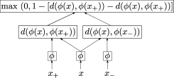
Figure 1: Trained siamese network

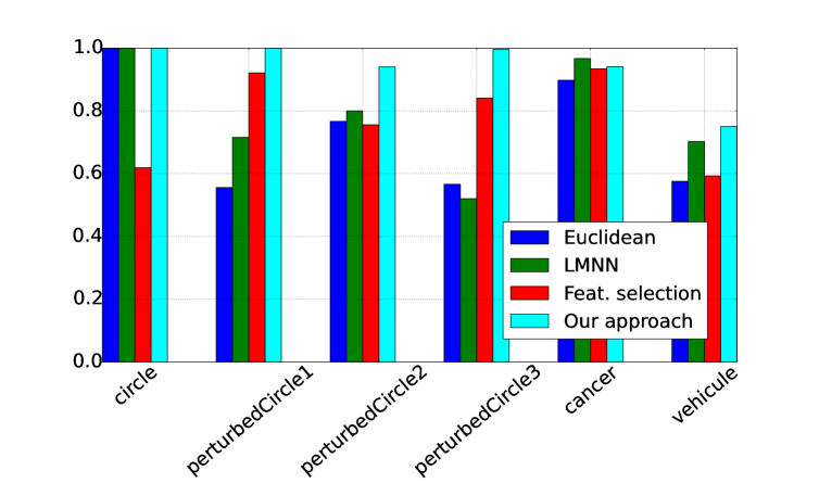
Figure 2: Classification accuracy of label propagation algorithm on $\epsilon$-graph depending on data set

In figure 2, we compare, for each dataset, the classification accuracy of the label propagation algorithm performed on the $\epsilon$-graph computed on the different representation spaces, with 20% of training instances. As expected, the euclidean distance and LMNN perform ideally on the circle data set, as the initial space is locally representative of the labelling similarity; however their performance decrease on artifical data sets as the initial description space is getting blurred and noisy, like for perturbedCircle1, perturbedCircle2 and perturbedCircle3 data sets. Feature selection algorithm performs well enough on perturbedCircle1 and perturbedCircle3 data set, where the labels are non-perturbed by the added features; however it does not surpass euclidean distance and LMNN algorithm for other data sets. On those artificial data sets, our algorithm performs either ideally or better than the other algorithms, and was able to learn a more representative projection space.

Concerning the real dataset cancer, the different algorithms perform quit well, broadly similar. Finally, on the vehicule dataset, we can see the interest of learning a projection space to obtain a better label propagation; yet the non-linear projection seems more adapted to the dataset complexity.

5 Conclusion

In this paper, we introduced an algorithm to learn a representation space for dataset that is adapted to a specific task. We defined and proved a first theoretical requirement for our algorithm to be optimal; what have been proved can easily be generalized to multi-layers neural network. Experiments on artificial and real data sets confirmed the relevance of our approach for solving classification task.

6 Acknowledgement

This work was partially supported by a grant from CPER Nord-Pas de Calais/FEDER DATA Advanced data science and technologies 2015-2020 and ANRT under the grant number CIFRE N^o 2013/0961

References

- Chopra et al. (2005) Sumit Chopra, Raia Hadsell, and Yann LeCun. Learning a similarity metric discriminatively, with application to face verification. In Proceedings of the 2005 IEEE Computer Society Conference on Computer Vision and Pattern Recognition (CVPR’05) - Volume 1 - Volume 01, CVPR ’05, pp. 539–546, Washington, DC, USA, 2005. IEEE Computer Society.
- Collobert et al. (2011) Ronan Collobert, Koray Kavukcuoglu, and Clement Farabet. Torch7: A Matlab-like Environment for Machine Learning. In BigLearn NIPS Workshop, 2011.
- de Sousa et al. (2013) Celso André R. de Sousa, Solange O. Rezende, and Gustavo E. A. P. A. Batista. Influence of graph construction on semi-supervised learning. In Hendrik Blockeel, Kristian Kersting, Siegfried Nijssen, and Filip Zelezný (eds.), ECML/PKDD (3), volume 8190 of Lecture Notes in Computer Science, pp. 160–175. Springer, 2013.
- (4) Paramveer S. Dhillon, Partha Pratim Talukdar, and Koby Crammer. Inference driven metric learning for graph construction.
- Geurts et al. (2006) Pierre Geurts, Damien Ernst, and Louis Wehenkel. Extremely randomized trees. Machine Learning, 63(1):3–42, 2006.
- He et al. (2013) Yujie He, Wenlin Chen, Yixin Chen, and Yi Mao. Kernel density metric learning. In Data Mining (ICDM), 2013 IEEE 13th International Conference on, pp. 271–280, Dec 2013.
- Hoffer & Ailon (2014) Elad Hoffer and Nir Ailon. Deep metric learning using triplet network. CoRR, abs/1412.6622, 2014.
- J. Weston (2008) R. Collobert. J. Weston, F. Ratle. Deep learning via semi-supervised embedding. In International Conference on Machine Learning, 2008.
- Jebara et al. (2009) T. Jebara, J. Wang, and S.F. Chang. Graph construction and b-matching for semi-supervised learning. In International Conference on Machine Learning, 2009.
- Kedem et al. (2012) Dor Kedem, Stephen Tyree, Kilian Weinberger, Fei Sha, and Gert Lanckriet. Non-linear metric learning. In P. Bartlett, F.C.N. Pereira, C.J.C. Burges, L. Bottou, and K.Q. Weinberger (eds.), Advances in Neural Information Processing Systems 25, pp. 2582–2590. 2012.
- Liu & Chang (2009) Wei Liu and Shih-Fu Chang. Robust multi-class transductive learning with graphs. In Computer Vision and Pattern Recognition, 2009. CVPR 2009. IEEE Conference on, pp. 381–388. IEEE, 2009.
- Maier et al. (2008) Markus Maier, Ulrike von Luxburg, and Matthias Hein. Influence of graph construction on graph-based clustering measures. In Advances in Neural Information Processing Systems 21, Proceedings of the Twenty-Second Annual Conference on Neural Information Processing Systems, Vancouver, British Columbia, Canada, December 8-11, 2008, pp. 1025–1032, 2008.
- Maier, Markus et al. (2013) Maier, Markus, von Luxburg, Ulrike, and Hein, Matthias. How the result of graph clustering methods depends on the construction of the graph. ESAIM: PS, 17:370–418, 2013.
- Rifai et al. (2011) Salah Rifai, Yann Dauphin, Pascal Vincent, Yoshua Bengio, and Xavier Muller. The manifold tangent classifier. In Advances in Neural Information Processing Systems 24: 25th Annual Conference on Neural Information Processing Systems 2011. Proceedings of a meeting held 12-14 December 2011, Granada, Spain., pp. 2294–2302, 2011.
- Vikas Sindhwani & Belkin (2005) Partha Niyogi Vikas Sindhwani and M. Belkin. Beyond the point cloud: from transductive to semi-supervised learning. In International Conference on Machine Learning (ICML), pp. 824–831, 2005.
- Weinberger & Saul (2009) Kilian Q. Weinberger and Lawrence K. Saul. Distance metric learning for large margin nearest neighbor classification. Journal of Machine Learning Research (JMLR), 10:207–244, June 2009.
- Zhou et al. (2004) Dengyong Zhou, Olivier Bousquet, Thomas N. Lal, Jason Weston, and Bernhard Schölkopf. Learning with local and global consistency. In S. Thrun, L.K. Saul, and B. Schölkopf (eds.), Advances in Neural Information Processing Systems 16, pp. 321–328. MIT Press, 2004.
- Zhu (2005) Xiaojin Zhu. Semi-supervised learning literature survey. Technical Report 1530, Computer Sciences, University of Wisconsin-Madison, 2005.
- Zhu & Ghahramani (2002) Xiaojin Zhu and Zoubin Ghahramani. Learning from labeled and unlabeled data with label propagation. Technical report, Carnegie Mellon University, 2002.
- Zhu et al. (2003) Xiaojin Zhu, Zoubin Ghahramani, and John D. Lafferty. Semi-supervised learning using gaussian fields and harmonic functions. In Machine Learning, Proceedings of the Twentieth International Conference (ICML 2003), August 21-24, 2003, Washington, DC, USA, pp. 912–919, 2003.