Critical two–point correlation functions and “equation of motion” in the $\varphi^{4}$ model

Abstract

Critical two–point correlation functions in the continuous and lattice $\varphi^{4}$ models with scalar order parameter $\varphi$ are considered. We show by different non–perturbative methods that the critical correlation functions $\langle\varphi^{n}({\bf 0})\varphi^{m}({\bf x})\rangle$ are proportional to $\langle\varphi({\bf 0})\varphi({\bf x})\rangle$ at $\mid{\bf x}\mid=x\to\infty$ for any positive odd integers $n$ and $m$. We investigate how our results and some other results for well–defined models can be related to the conformal field theory (CFT), considered by Rychkov and Tan, and reveal some problems here. We find this CFT to be rather formal, as it is based on an ill–defined model. Moreover, we find it very unlikely that the used there “equation of motion” really holds from the point of view of statistical physics.

Keywords: $\varphi^{4}$ model, correlation functions, conformal field theory, operators

1 Introduction

In this paper we investigate non–perturbatively the relations between different two–point correlation functions in the scalar $\varphi^{4}$ model from the point of view of statistical physics. We consider correlation functions $\langle\varphi^{n}({\bf 0})\varphi^{m}({\bf x})\rangle$ with positive integer powers $n$ and $m$ of the local order parameter $\varphi({\bf x})$ at the critical point. For odd values of $n$ and $m$, we find that all these correlation functions are asymptotically proportional to $\langle\varphi({\bf 0})\varphi({\bf x})\rangle$ at large distances $\mid{\bf x}\mid\to\infty$. Although this result may seem to be very simple, it has some fundamental importance when we try to relate the results of the conformal field theory [1, 2, 3] with those, which can be obtained purely from statistical physics.

We consider the continuous $\varphi^{4}$ model in the thermodynamic limit of diverging volume $V\to\infty$ with the Hamiltonian $\cal{H}$ given by

$$\frac{\cal{H}}{k_{B}T}=\int\left(r_{0}\varphi^{2}({\bf x})+c(\nabla\varphi({\bf x}))^{2}+u\varphi^{4}({\bf x})\right)d{\bf x}\;,$$ (1)

where $\varphi({\bf x})$ is the scalar order parameter, depending on the coordinate ${\bf x}$, $T$ is the temperature, $k_{B}$ is the Boltzmann constant, whereas $r_{0}$, $c$ and $u$ are Hamiltonian parameters, which are functions of $T$. It is assumed that there exists the upper cut-off parameter $\Lambda$ for the Fourier components of the order-parameter field $\varphi({\bf x})$. Namely, the Fourier–transformed Hamiltonian reads

$$\frac{\cal{H}}{k_{B}T}=\sum\limits_{\bf k}\left(r_{0}+c\,{\bf k}^{2}\right){\mid\varphi_{\bf k}\mid}^{2}+uV^{-1}\sum\limits_{{\bf k}_{1},{\bf k}_{2},{\bf k}_{3}}\varphi_{{\bf k}_{1}}\varphi_{{\bf k}_{2}}\varphi_{{\bf k}_{3}}\varphi_{-{\bf k}_{1}-{\bf k}_{2}-{\bf k}_{3}}\;,$$ (2)

where $\varphi_{\bf k}=V^{-1/2}\int\varphi({\bf x})\exp(-i{\bf kx})\,d{\bf x}$ and $\varphi({\bf x})=V^{-1/2}\sum\limits_{k<\Lambda}\varphi_{\bf k}\exp(i{\bf kx})$. Moreover, the only allowed configurations of $\varphi({\bf x})$ are those, for which $\varphi_{\bf k}=0$ holds at $k\equiv\mid{\bf k}\mid>\Lambda$. This is the limiting case $m\to\infty$ of the model where all configurations are allowed, but Hamiltonian (2) is completed by the term $\sum_{\bf k}\left(k/\Lambda\right)^{2m}\mid\varphi_{{\bf k}}\mid^{2}$.

We consider also the lattice version of the scalar $\varphi^{4}$ model with the Hamiltonian

$$\frac{\mathcal{H}}{k_{B}T}=-\beta\sum\limits_{\langle ij\rangle}\varphi({\bf x}_{i})\varphi({\bf x}_{j})+\sum\limits_{i}\left(\varphi^{2}({\bf x}_{i})+\lambda\left(\varphi^{2}({\bf x}_{i})-1\right)^{2}\right)\;,$$ (3)

where $-\infty<\varphi({\bf x}_{i})<\infty$ is a continuous scalar order parameter at the $i$-th lattice site with coordinate ${\bf x}_{i}$, and $\langle ij\rangle$ denotes the set of all nearest neighbors.

The considered here versions of the $\varphi^{4}$ model are standard and widely used in numerous analytical and numerical studies – see, e. g. [4, 5, 6, 7, 8, 9, 10, 11, 12] and references therein.

2 The critical two–point correlation functions above the
upper critical dimension

It is well known [4, 5, 6, 7, 8] that the critical behavior of the $\varphi^{4}$ model (1) above the upper critical spatial dimension $d$, i. e., at $d>4$, is determined by the Gaussian fixed point $r_{0}=0$ and $u=0$. It means that the critical correlations functions at $\mid{\bf x}\mid\to\infty$ can be exactly calculated from the Gaussian model with Hamiltonian

$$\frac{\cal{H}}{k_{B}T}=\int c\,(\nabla\varphi)^{2}d{\bf x}=\sum\limits_{{\bf k},\,k<\Lambda}c\,{\bf k}^{2}{\mid\varphi_{\bf k}\mid}^{2}\;.$$ (4)

In the Gaussian model, the correlation functions $\langle\varphi^{n}({\bf x}_{1})\varphi^{m}({\bf x}_{2})\rangle$ can be exactly calculated by coupling the variables according to the Wick’s theorem. The calculations can be performed either for Fourier transforms or directly for the real–space correlation functions. In the latter case, one has to consider diagrams, constructed from one vertex with $n$ lines at coordinate ${\bf x}_{1}$ and one vertex with $m$ lines at coordinate ${\bf x}_{2}$. The correlation function $\langle\varphi^{n}({\bf x}_{1})\varphi^{m}({\bf x}_{2})\rangle$ is given by the sum of all diagrams, obtained by coupling the lines. In this diagram technique, a line starting at coordinate ${\bf x}_{1}$ and ending at coordinate ${\bf x}_{2}$ gives the factor $\langle\varphi({\bf x}_{1})\varphi({\bf x}_{2})\rangle$. A line can start and end at the same point, in which case it gives the factor $\langle\varphi^{2}({\bf x})\rangle\equiv\langle\varphi^{2}\rangle$ for any ${\bf x}$. Taking into account the combinatorial factors for different couplings, we obtain

$$\langle\varphi^{n}({\bf 0})\varphi^{m}({\bf x})\rangle=\sum\limits_{\ell}\frac{n!\,m!}{\ell!\,[(n-\ell)/2]!\,[(m-\ell)/2]!}\left(\frac{\langle\varphi^{2}\rangle}{2}\right)^{(n+m-2\ell)/2}\langle\varphi({\bf 0})\varphi({\bf x})\rangle^{\ell}\;,$$ (5)

where $\ell$ is an odd integer within $1\leq\ell\leq\min\{n,m\}$ for odd $n$ and $m$. Similarly, $\ell$ is an even integer within $0\leq\ell\leq\min\{n,m\}$ for even $n$ and $m$. If $n$ is odd and $m$ is even or vice versa, then the coupling of all lines is not possible, and the correlation function is zero.

The Fourier–transformed two–point correlation function of the Gaussian model (4) is well known to be $G({\bf k})=\langle\mid\varphi_{\bf k}\mid^{2}\rangle=1/(2ck^{2})$. It means that $\langle\varphi({\bf 0})\varphi({\bf x})\rangle\propto x^{2-d}$ holds at $x=\mid{\bf x}\mid\to\infty$. Thus, we conclude from Eq. (5) that $\langle\varphi^{n}({\bf 0})\varphi^{m}({\bf x})\rangle$ is proportional to $\langle\varphi({\bf 0})\varphi({\bf x})\rangle$ at $x\to\infty$ for positive odd integers $n$ and $m$, whereas the asymptotic behavior is $\propto(const+\langle\varphi({\bf 0})\varphi({\bf x})\rangle^{2})$ for positive even integers $n$ and $m$. In particular,

$$\langle\varphi^{n}({\bf 0})\varphi^{m}({\bf x})\rangle=n!!\,m!!\,\langle\varphi^{2}\rangle^{(n+m-2)/2}\,\langle\varphi({\bf 0})\varphi({\bf x})\rangle+O\left(x^{6-3d}\right)$$ (6)

holds for any positive odd integers $n$ and $m$ at $x\to\infty$, where $n!!=1\cdot 3\cdot 5\cdots n$, except that the remainder term $O\left(x^{6-3d}\right)$ exactly vanishes for $n=1$ and/or $m=1$.

3 The two–point joint probability density and
correlation functions

All correlation functions $\langle\varphi^{n}({\bf 0})\varphi^{m}({\bf x})\rangle$ in the $\varphi^{4}$ model (1) (and not only in such a model) can be calculated, if we know the two–point joint probability density $\mathcal{P}_{2}(\varphi_{1},\varphi_{2},{\bf x}_{1},{\bf x}_{2})$. In this notation, $\mathcal{P}_{2}(\varphi_{1},\varphi_{2},{\bf x}_{1},{\bf x}_{2})d\varphi_{1}d\varphi_{2}$ is the probability that $\varphi({\bf x}_{1})\in[\varphi_{1},\varphi_{1}+d\varphi_{1}]$ and $\varphi({\bf x}_{2})\in[\varphi_{2},\varphi_{2}+d\varphi_{2}]$ at $d\varphi_{1}\to 0$ and $d\varphi_{2}\to 0$. Consequently, we have

$$\langle\varphi^{n}({\bf x}_{1})\varphi^{m}({\bf x}_{2})\rangle=\int\limits_{-\infty}^{\infty}\int\limits_{-\infty}^{\infty}\varphi_{1}^{n}\varphi_{2}^{m}\,\mathcal{P}_{2}(\varphi_{1},\varphi_{2},{\bf x}_{1},{\bf x}_{2})\,d\varphi_{1}d\varphi_{2}\;.$$ (7)

It is convenient to represent the two–point joint probability density as

$$\mathcal{P}_{2}(\varphi_{1},\varphi_{2},{\bf x}_{1},{\bf x}_{2})=\mathcal{P}_{1}(\varphi_{1})\mathcal{P}_{1}(\varphi_{2})+\mathcal{F}(\varphi_{1},\varphi_{2},\mid{\bf x}_{1}-{\bf x}_{2}\mid)\;,$$ (8)

where $\mathcal{P}_{1}(\varphi)$ is the one–point probability density ($\mathcal{P}_{1}(\varphi)d\varphi$ is the probability that $\varphi({\bf x})\in[\varphi,\varphi+d\varphi]$ at $d\varphi\to 0$ for any coordinate ${\bf x}$). The spatial dependence is represented in terms of $\mid{\bf x}_{1}-{\bf x}_{2}\mid$ owing to the translational and rotational symmetry of the model. Moreover, we have $\mathcal{F}(\varphi_{1},\varphi_{2},x)\to 0$ at $x\to\infty$, since the correlations vanish at infinitely large distances. Inserting (8) into (7) at ${\bf x}_{1}={\bf 0}$ and ${\bf x}_{2}={\bf x}$, we obtain

$$\langle\varphi^{n}({\bf 0})\varphi^{m}({\bf x})\rangle-\langle\varphi^{n}\rangle\langle\varphi^{m}\rangle=\int\limits_{-\infty}^{\infty}\int\limits_{-\infty}^{\infty}\varphi_{1}^{n}\varphi_{2}^{m}\,\mathcal{F}(\varphi_{1},\varphi_{2},\mid{\bf x}\mid)\,d\varphi_{1}d\varphi_{2}\;.$$ (9)

According to the symmetry of the model, we have $\mathcal{P}_{1}(\varphi)=\mathcal{P}_{1}(-\varphi)$, $\mathcal{P}_{2}(\varphi_{1},\varphi_{2},{\bf x}_{1},{\bf x}_{2})=\mathcal{P}_{2}(-\varphi_{1},-\varphi_{2},{\bf x}_{1},{\bf x}_{2})$ and $\mathcal{P}_{2}(\varphi_{1},\varphi_{2},{\bf x}_{1},{\bf x}_{2})=\mathcal{P}_{2}(\varphi_{2},\varphi_{1},{\bf x}_{1},{\bf x}_{2})$. Eq. (8) then implies $\mathcal{F}(\varphi_{1},\varphi_{2},x)=\mathcal{F}(-\varphi_{1},-\varphi_{2},x)$ and $\mathcal{F}(\varphi_{1},\varphi_{2},x)=\mathcal{F}(\varphi_{2},\varphi_{1},x)$.

We need some more specific properties of $\mathcal{F}(\varphi_{1},\varphi_{2},x)$ for our analysis. The above relations imply that $\mathcal{F}(0,\varphi_{2},x)=\mathcal{F}(0,-\varphi_{2},x)$ holds. This symmetry with respect to the argument $\varphi_{2}$ does not hold for a fixed $\varphi_{1}\neq 0$. It is quite natural to assume that this symmetry is broken in such a way that

$$\mathcal{F}(\varphi_{1},\varphi_{2},x)>\mathcal{F}(\varphi_{1},-\varphi_{2},x)\qquad\mbox{for }\varphi_{1}>0\;\mbox{and }\varphi_{2}>0$$ (10)

holds due to the interactions of ferromagnetic type in the $\varphi^{4}$ model. Indeed, if a spin at a given coordinate is oriented up ($\varphi_{1}>0$) then it is energetically preferable and more probable that another spin at any finite distance $x$ from it is also oriented up, in such a way that the inequality (10) is satisfied.

According to the current knowledge about the critical phenomena, the two–point correlation functions are representable by an expansion in powers of $x$ at the critical point, and sometimes also the logarithmic corrections appear. Therefore, it is natural to assume that $\mathcal{F}(\varphi_{1},\varphi_{2},x)$ can be expanded as

$$\mathcal{F}(\varphi_{1},\varphi_{2},x)=\sum\limits_{(i,j)\in\Omega}A_{ij}(\varphi_{1},\varphi_{2})\,x^{-\lambda_{i}}(\ln x)^{\mu_{ij}}$$ (11)

at $x\to\infty$, where $A_{ij}$ are the expansion coefficients, and the sum runs over pairs of indices $(i,j)$ belong to some set $\Omega\subset\mathbb{N}^{2}$.

Let us $i=j=0$ correspond to the leading term. The condition (10) is satisfied at $x\to\infty$, if it is satisfied for this leading expansion term. Formally, it is also satisfied in this limit if the asymmetry, stated in (10), first shows up in some term with indices $i^{*}$ and $j^{*}$, whereas all lower–order terms are symmetric, implying that $A_{ij}(\varphi_{1},\varphi_{2})=A_{ij}(\varphi_{1},-\varphi_{2})=A_{ij}(-\varphi_{1},\varphi_{2})$ holds for these terms. The case, where the leading term is asymmetric is also included, and it corresponds to $i^{*}=j^{*}=0$. Consider now odd $n$ and $m$. In this case, inserting (11) into (9), the symmetric terms give vanishing result, whereas the leading asymptotic behavior is provided by the term with indices $i^{*}$ and $j^{*}$, for which we have

$$A_{i^{*}j^{*}}(\varphi_{1},\varphi_{2})>A_{i^{*}j^{*}}(\varphi_{1},-\varphi_{2})\qquad\mbox{for }\varphi_{1}>0\;\mbox{and }\varphi_{2}>0$$ (12)

according to (10). Thus, we obtain

$$\langle\varphi^{n}({\bf 0})\varphi^{m}({\bf x})\rangle=B_{nm}\,x^{-\lambda_{i^{*}}}(\ln x)^{\mu_{i^{*}j^{*}}}\qquad\mbox{at}\quad x\to\infty$$ (13)

for odd $n$ and $m$, where $B_{nm}$ are positive coefficients given by

$$B_{nm} = \int\limits_{-\infty}^{\infty}\int\limits_{-\infty}^{\infty}\varphi_{1}^{n}\varphi_{2}^{m}A_{i^{*}j^{*}}(\varphi_{1},\varphi_{2})d\varphi_{1}d\varphi_{2}$$ (14)

$$= 2\int\limits_{0}^{\infty}\varphi_{1}^{n}d\varphi_{1}\int\limits_{0}^{\infty}\varphi_{2}^{m}\left[A_{i^{*}j^{*}}(\varphi_{1},\varphi_{2})-A_{i^{*}j^{*}}(\varphi_{1},-\varphi_{2}\right)]d\varphi_{2}>0\;.$$

The positiveness of $B_{nm}$ follows from (12) and implies that

$$\langle\varphi^{n}({\bf 0})\varphi^{m}({\bf x})\rangle=C_{nm}\,\langle\varphi({\bf 0})\varphi({\bf x})\rangle\qquad\mbox{at}\quad x\to\infty$$ (15)

holds with $C_{nm}=B_{nm}/B_{11}>0$ for any positive odd integers $n$ and $m$. This result is a generalization of those in Sec. 2 to any spatial dimension, at which the critical point of the second-order phase transition exists.

The actual consideration can be trivially extended to the lattice version of the scalar $\varphi^{4}$ model. Indeed, all relations of this section can be applied to the correlation functions $\langle\varphi^{n}({\bf 0})\varphi^{m}({\bf x})\rangle$ with ${\bf x}$ oriented along any given crystallographic direction in the lattice. Only the coefficients can depend on the particular lattice and crystallographic direction. Moreover, the two–point correlation functions are isotropic at large distances $x\to\infty$, so that the asymptotic relation (15) refers also to the lattice model, $C_{nm}$ being isotropic.

4 Results of Monte Carlo simulation

We have performed Monte Carlo (MC) simulations for the lattice $\varphi^{4}$ model (3) in two dimensions. Let us denote by $G_{n}({\bf k})$ the Fourier transform of the two–point correlation function $\langle\varphi^{n}({\bf 0})\varphi^{n}({\bf x})\rangle$. It is calculated as $G_{n}({\bf k})=\langle\mid v_{n}({\bf k})\mid^{2}\rangle$, where $v_{n}({\bf k})$ is the Fourier transform of $\tilde{v}_{n}({\bf x})=\varphi^{n}({\bf x})$, i. e., $v_{n}({\bf k})=N^{-1/2}\sum_{\bf x}\tilde{v}_{n}({\bf x})\exp(-i{\bf kx})$, where $N=L^{2}$ is the number of sites in the 2D square lattice with dimensions $L\times L$. The MC simulations at Hamiltonian parameters $\lambda=1$ and $\beta=0.680605$ have been performed, where the chosen value of $\beta$ is consistent with the critical value $\beta_{c}=0.680605\pm 0.000004$ estimated in [13]. The Fourier transforms $G_{n}({\bf k})$ in the $\langle 10\rangle$ crystallographic direction have been evaluated at $n=1,2,3$ for different lattice sizes $L=128,256,512$ and $768$, using the techniques described in [13] with the only generalization $\varphi({\bf x})\to\tilde{v}_{n}({\bf x})$ and $\varphi_{\bf k}\to v_{n}({\bf k})$. The obtained $\ln G_{n}({\bf k})$ vs $\ln k$ plots are shown in Fig. 1.

Figure 1: The $\ln G_{n}({\bf k})$ vs $\ln k$ plots at $n=1$ (solid symbols, upper plots), $n=2$ (solid symbols, lower plots) and $n=3$ (empty symbols, upper plots) for different lattice sizes – $L=128$ (triangles), $L=256$ (squares), $L=512$ (diamonds) and $L=768$ (circles). The straight dashed line indicates the small–$k$ asymptotic behavior of $\ln G_{3}({\bf k})$ at $L\to\infty$.

Although the simulations have been performed at an approximate value of $\beta_{c}$, our techniques allow us to recalculate the data for slightly different $\beta$, using the Taylor series. Thus we have verified that the error $\pm 0.000004$ in the $\beta_{c}$ value is insignificant, i. e., it causes systematic deviations in the plots of Fig. 1, which are much smaller than the symbol size. We can see from these plots that the behavior of $G_{3}({\bf k})$ is very similar to that of $G_{1}({\bf k})$ at small enough $k$ values, i. e., the corresponding log–log plots are practically parallel to each other for a given lattice size $L$. Some finite–size effects are observed, in such a way that these plots converge to a curve with asymptotic slope $-7/4$ at $L\to\infty$, as indicated by a dashed line in Fig. 1. It is consistent with the well known $G_{1}({\bf k})\propto k^{-2+\eta}=k^{-7/4}$ asymptotic critical behavior in the models of 2D Ising universality class.

In fact, the MC data suggest that $G_{3}({\bf k})\propto G_{1}({\bf k})$ holds at $k\to 0$, which corresponds to $\langle\varphi^{3}({\bf 0})\varphi^{3}({\bf x})\rangle\propto\langle\varphi({\bf 0})\varphi({\bf x})\rangle$ at $x\to\infty$, in agreement with (15). To the contrary, the slope of $\ln G_{2}({\bf k})$ vs $\ln k$ plot is much smaller than that of $\ln G_{1}({\bf k})$ vs $\ln k$ plot for small $k$ values, indicating that $\langle\varphi^{2}({\bf 0})\varphi^{2}({\bf x})\rangle-\langle\varphi^{2}\rangle^{2}$ decays much faster than $\langle\varphi({\bf 0})\varphi({\bf x})\rangle$ at $x\to\infty$ and the proportionality relation (15) does not hold for even exponents $n$ and $m$.

5 Some results of the conformal field theory

In this section we will briefly review and critically discuss recent results of the conformal field theory (CFT) reported in [1]. A method is proposed in this work to recover the $\epsilon$–expansion from CFT. The operators $V_{n}\equiv(\varphi^{n})_{\mathrm{WF}}$ are considered in the critical $\varphi^{4}$ theory, where $(\varphi^{n})_{\mathrm{WF}}$ is the operator $\varphi^{n}$ at the Wilson–Fisher (WF) fixed point in $d=4-\epsilon$ dimensions ($\epsilon>0$). The notation $V_{n}$ is used to distinguish the operators at the WF fixed point from the free theory operators $\varphi^{n}$. As claimed in [1], all operators $\varphi^{n}$ of the free theory are primaries, whereas $V_{3}$ is not a primary, since it is related to $V_{1}$ via certain equation of motion.

The following axioms are formulated in [1] as cornerstones of the proposed approach:

1. The WF fixed point is conformally invariant.

2. Correlation functions of operators at the WF fixed point approach free theory correlators in the limit $\epsilon\to 0$.

3. Operators $V_{n}$, $n\neq 3$, are primaries. Operator $V_{3}$ is not a primary but is proportional to $\partial^{2}V_{1}$:

   $$\partial^{2}V_{1}=\alpha V_{3}\;.$$ (16)

The coefficient $\alpha$ is unknown at this stage, but later it is found by fitting the correlator $\langle V_{3}({\bf 0})V_{3}({\bf x})\rangle$ to the free theory correlator $\langle\varphi^{3}({\bf 0})\varphi^{3}({\bf x})\rangle$ in four dimensions at $\epsilon\to 0$.

The two–point correlation functions in this CFT behave as

$$\langle V_{n}({\bf 0})V_{m}({\bf x})\rangle=B_{nm}\,x^{-\Delta_{n}-\Delta_{m}}$$ (17)

at the WF fixed point, where $B_{nm}$ are coefficients (which are zero in a subset of cases), whereas $\Delta_{n}$ is the dimension of operator $V_{n}$, which can be expressed as

$$\Delta_{n}=n\delta+\gamma_{n}\;,$$ (18)

where $\delta=1-\epsilon/2$ is the free scalar dimension and $\gamma_{n}$ is the anomalous dimension of operator $V_{n}$. Moreover, $\gamma_{n}\to 0$ holds at $\epsilon\to 0$.

Eq. (17) represents a clearly different scaling form than (15). A resolution of this puzzle is such that (17) refers to a formal treatment of a different $\varphi^{4}$ model which, contrary to our case, does not contain any upper cut–off for wave vectors. It formally ensures that the scaling can be exactly scale–free, i. e., described exactly by a power law. Note that the upper cut–off ($k<\Lambda$) gives certain length scale $1/\Lambda$, so that the real–space correlation functions appear to be only asymptotically (at $x\to\infty$) scale–free at the critical point and even at the renormalization group (RG) fixed point in a model with finite $\Lambda$. Indeed, Eq. (17) cannot hold at $x\to 0$ in such a model, since finite $\Lambda$ ensures that the local quantities $\langle V_{n}({\bf 0})V_{m}({\bf 0})\rangle$ are also finite.

Note that an exact power law is observed in the usual Wilson–Fisher renormalization in the wave–vector space, however, only for the Fourier–transformed two–point correlation function $G({\bf k})$. It behaves as $G({\bf k})=ak^{-2+\eta}$ within $0<k<\Lambda$ at the Wilson–Fisher fixed point owing to the well–known rescaling rule $G({\bf k},\mu)=s^{2-\eta}G(s{\bf k},R_{s}\mu)$ [5]. Here $\mu$ is a point in the parameter space of the Hamiltonian. This point is varied under the RG transformation $R_{s}$. The real–space correlation function $\tilde{G}({\bf x})$ can be straightforwardly calculated from $G({\bf k})=ak^{-2+\eta}$ via $\tilde{G}({\bf x})=(2\pi)^{-d}\int_{k<\Lambda}G({\bf k})\exp(i{\bf kx})d^{d}k$ to aware that it does not follow an exact power law.

Apparently, the absence of any length scale is a desired property in CFT. Unfortunately, the model without any cut–off is ill–defined, since the local quantities $\langle V_{2n}({\bf x})\rangle$ ($n\geq 1$) are divergent. Moreover, no mathematically justified calculations can be performed in this case even in the Gaussian model because of the divergent quantity $\langle\varphi^{2}\rangle$ appearing in (5). Recall that a “tadpole” is formed when two lines of the same vertex are coupled, and it gives the factor $\langle\varphi^{2}\rangle$. Obviously, the free theory calculations at $d=4$ are performed in [1], omitting the divergent diagrams with tadpoles in the Gaussian model without any cut–off. Only in this case we can obtain the reported in [1] results, $\langle\varphi({\bf 0})\varphi({\bf x})\rangle=x^{-2}$ and $\langle\varphi^{3}({\bf 0})\varphi^{3}({\bf x})\rangle=x^{-6}$, after certain normalization of $\varphi$. Such a subtraction of divergent terms is, in fact, a well known idea of the perturbative renormalization. From this point of view, the approach of [1] is neither rigorous nor really non–perturbative.

We think that the only way how this formal CFT can be justified is to find a strict relation between this formal treatment and the results of a well defined model. Such possible relations are discussed in Sec. 6.

Another question is the validity of the “equation of motion” (16). In the $\varphi^{4}$ model, each configuration $\{\varphi\}$ of the order parameter field $\varphi({\bf x})$ shows up with the statistical weight $Z^{-1}\exp[-\mathcal{H}(\{\varphi\})/(k_{B}T)]$, where $Z$ is the partition function. Therefore, it is impossible that a constraint of the form (16) is really satisfied, unless any local violation of such a constraint leads to a divergent local Hamiltonian density $h({\bf x})$. To aware about this, we can consider a configuration $\{\varphi\}$, which obeys (16), and another configuration $\{\varphi\}^{\prime}$. Let us $\{\varphi\}^{\prime}=\{\varphi\}$ holds everywhere, except a local region ${\bf x}\in\Omega$, where $\{\varphi\}^{\prime}$ does not satisfy (16). The ratio of statistical weights for $\{\varphi\}^{\prime}$ and $\{\varphi\}$ is $Z^{-1}\exp[-\Delta\mathcal{H}(\{\varphi\})/(k_{B}T)]$, where $\Delta\mathcal{H}=\int_{{\bf x}\in\Omega}(h^{\prime}({\bf x})-h({\bf x}))d{\bf x}$, $h({\bf x})$ and $h^{\prime}({\bf x})$ being Hamiltonian densities for configurations $\{\varphi\}$ and $\{\varphi\}^{\prime}$, respectively. If (16) really holds, then the configuration $\{\varphi\}^{\prime}$ must show up with a vanishing statistical weight as compared to that of $\{\varphi\}$, i. e., the above mentioned ratio must be zero. Obviously, it is possible only if $h^{\prime}({\bf x})$ is divergent at least within a subregion of $\Omega$.

On the other hand, there are no evidences that the density of renormalized Hamiltonian contains any term which is divergent if (16) is violated. Particularly, the usual perturbative approximations for the fixed–point Hamiltonian in $4-\epsilon$ dimensions suggest that the renormalized Hamiltonian is just the same as the bare one (1) with the only difference that the Hamiltonian parameters have special, i. e., renormalized values. The density of such renormalized Hamiltonian is finite for relevant field configurations with $\mid\nabla\varphi({\bf x})\mid<\infty$ and $\mid\varphi({\bf x})\mid<\infty$.

6 Possible relations of formal CFT to well defined models

A standard way to compare the results of the lattice $\varphi^{4}$ model to those of CFT is to redefine operators of the lattice model. In particular, $\varphi^{3}$ has to be replaced by $W_{3}=\varphi^{3}+b\varphi$, where an appropriate value of the constant $b$ is chosen to cancel the $\langle\varphi({\bf 0})\varphi({\bf x})\rangle$ contribution contained in $\langle\varphi^{3}({\bf 0})\varphi^{3}({\bf x})\rangle$. In this case, the operator $\varphi\equiv W_{1}$ remains unaltered. We have verified perturbatively that the same method works also in the considered here continuous $\varphi^{4}$ model with cut–off for wave vectors. Namely, the perturbative expansion in powers of $x^{-2}$, $\ln x$ and $\epsilon$ is such that the terms with $x^{-2}$ (and logarithmic correction factors) cancel in $\langle W_{1}({\bf 0})W_{3}({\bf x})\rangle$ and the terms with both $x^{-2}$ and $x^{-4}$ cancel in $\langle W_{3}({\bf 0})W_{3}({\bf x})\rangle$ at the RG fixed point, if $b$ is chosen as $b=-C_{13}$, where $C_{13}$ is the coefficient in (15). We have examined the corresponding expansion in powers of $k^{2}$, $\ln k$ and $\epsilon$ for the Fourier transforms of these correlators, using the standard representation of $G({\bf k})$ by self-energy diagrams, to verify that the above mentioned cancellations take place in all orders of the perturbation theory. It ensures that the expected $\propto x^{-\Delta_{1}-\Delta_{3}}$ asymptotic behavior of $\langle W_{1}({\bf 0})W_{3}({\bf x})\rangle$ and the expected $\propto x^{-2\Delta_{3}}$ asymptotic behavior of $\langle W_{3}({\bf 0})W_{3}({\bf x})\rangle$ can be, in principle, consistent with the perturbation theory, since $\Delta_{n}\to n$ at $\epsilon\to 0$.

We have tested also two–point correlators of odd operators $W_{1}\equiv\varphi$, $W_{3}=\varphi^{3}+b\varphi$ and $W_{5}=\varphi^{5}+b_{1}\varphi+b_{3}\varphi^{3}$. Unfortunately, this method becomes problematic if operators $W_{2m+1}$ with $m>1$ are included, since the number of required cancellations increase more rapidly than the number of free coefficients. Note that terms with $x^{-2}$ and $x^{-4}$ have to be canceled in $\langle W_{1}({\bf 0})W_{5}({\bf x})\rangle$, terms with $x^{-2}$, $x^{-4}$ and $x^{-6}$ have to be canceled in $\langle W_{3}({\bf 0})W_{5}({\bf x})\rangle$, and terms with $x^{-2}$, $x^{-4}$, $x^{-6}$ and $x^{-8}$ have to be canceled in $\langle W_{5}({\bf 0})W_{5}({\bf x})\rangle$. We have found it already impossible to reach all the necessary cancellations up to the $O\left(\epsilon^{2}\right)$ order for all two–point correlators of the above mentioned three operators $W_{1}$, $W_{3}$ and $W_{5}$. Hence, the finding of a precise relation between a well–defined continuous $\varphi^{4}$ model and the formal CFT treatment of [1] is at least problematic within the perturbation theory. The details of our perturbative calculations are given in Appendix.

It is interesting to look for a possible non–perturbative relation between the discussed here formal CFT and a well–defined model. The reported in [2] agreement of the results of the conformal bootstrap method with the known exact spectrum of the operator dimensions in the 2D Ising model is a good evidence for the existence of such a relation in two dimensions.

A nontrivial MC evidence for the existence of conformal symmetry in three dimensions has been provided in [14]. Another interesting MC test has been performed in [15] to check whether or not relations for amplitudes of correlation lengths, analogous to those predicted by CFT in the 2D Ising model, can be found in the 3D Ising model and, more generally, in the $O(n)$–symmetric models in three dimensions. Surprisingly, such a relation has been indeed obtained, however, only for anti-periodic boundary conditions and not for periodic ones, for which this relation exists in two dimensions. It reveals a qualitative difference between the two–dimensional and three–dimensional cases. According to this result, the following judgment can be made: even if the conformal symmetry exists in the 3D Ising model, then it is, however, questionable whether or not (or in which sense) the spatial dimensionality $d$ can be considered as a continuous parameter in the CFT. On the other hand, $d$ appears as a continuous parameter in the particular treatment of CFT in [1], since it is possible to recover the $\epsilon$–expansion from it.

Despite of the discussed here problems, the critical exponents provided by this CFT appear to be very well consistent with the currently accepted values of the 3D Ising model. In particular, $\eta=0.03631(3)$, $\nu=0.62999(5)$ and $\omega=0.8303(18)$ are reported in [2], in close agreement with the MC estimates $\eta=0.03627(10)$, $\nu=0.63002(10)$ and $\omega=0.832(6)$ of Hasenbusch [12]. These MC results have been obtained from the data for linear lattice sizes $L\leq 360$. We have tested the exponent $\eta$, evaluated from the susceptibility ($\chi$) data for much larger lattice sizes up to $L=2560$. The $\chi/L^{2}$ data at certain pseudocritical couplings $\widetilde{\beta}_{c}(L)$ (tending to the true critical coupling $\beta_{c}$ at $L\to\infty$ and corresponding to $U=\langle m^{4}\rangle/\langle m^{2}\rangle^{2}=1.6$, where $m$ is the magnetization per spin) for $L\leq 1536$ are given in [16]. Here we add more recent results: $\chi/L^{2}=1.1882(20)$ for $L=1728$, $\chi/L^{2}=1.1741(27)$ for $L=2048$ and $\chi/L^{2}=1.1669(28)$ for $L=2560$, obtained by the same techniques as before. The effective critical exponent $\eta_{\mathrm{eff}}(L)$ is obtained by fitting the data to the ansatz $\chi/L^{\prime 2}=aL^{\prime-\eta}$ within $L^{\prime}\in[L/2,2L]$. It is expected that $\eta_{\mathrm{eff}}(L)-\eta\propto L^{-\omega}$ holds at $L\to\infty$, where $\omega$ is the correction–to–scaling exponent. Surprisingly, we observe that $\eta_{\mathrm{eff}}$ vs $L^{-\omega}$ behavior shows the best linearity for large lattice sizes at $\omega=0.16(36)$ rather than at $\omega=0.8303(18)$. The plots of $\eta_{\mathrm{eff}}(L)$ depending on $L^{-0.16}$ and $L^{-0.8303}$ are shown in Fig. 2, where the value $\eta=0.03631(3)$ of [2] is indicated by dotted lines.

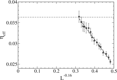
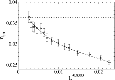
Figure 2: The effective exponent $\eta_{\mathrm{eff}}(L)$ depending on $L^{-0.16}$ (left) and $L^{-0.8303}$ (right). The dashed straight lines represent the linear fit (left) and a guide to eye (right). The value $\eta=0.03631(3)$ of [3] is indicated by dotted lines.

Although the agreement of this value with currently accepted ones is very good, it would be not superfluous to make further tests in order to see whether $\eta_{\mathrm{eff}}(L)$ really converges to $\eta=0.03631(3)$ or, perhaps, to a larger value, as it is suggested by an extrapolation of plots (dashed lines) in Fig. 2. It would be also very useful to obtain a more precise value of $\omega$ from large lattice sizes to see whether or not this value is indeed remarkably smaller than $0.83$. The latter possibility is strongly supported by our recent analytical results [13], from which $\omega\leq(\gamma-1)/\nu\approx 0.38$ is expected.

The referred here critical exponents $\eta=0.03631(3)$, $\nu=0.62999(5)$ and $\omega=0.8303(18)$ have been obtained in [2] based on the following hypotheses:

1. There exists a sharp kink on the border of the two–dimensional region of the allowed values of the operator dimensions $\Delta_{\sigma}=(1+\eta)/2$ and $\Delta_{\epsilon}=3-1/\nu$;

2. Critical exponents of the 3D Ising model correspond just to this kink.

If the hypothesis (i) about the existence of a sharp kink is true, then this kink, probably, has a special meaning for the 3D Ising model. Its existence, however, is not evident.

Figure 3: The values of $\Delta(\sigma)$, corresponding to the minimum (solid circles) and the “kink” (empty circles) in the plots of Fig. 7 in [2] depending on $N^{-3}$. The dashed lines show linear extrapolations.

According to the conjectures of [2], such a kink is formed at $N\to\infty$, where $N$ is the number of derivatives included into the analysis. As discussed in [2], it implies that the minimum in the plots of Fig. 7 in [2] should be merged with the apparent “kink” at $N\to\infty$. This “kink” is not really sharp at a finite $N$. Nevertheless, its location can be identified with the value of $\Delta(\sigma)$, at which the second derivative of the plot has a local maximum. The minimum of the plot is slightly varied with $N$, whereas the “kink” is barely moving [2]. Apparently, the convergence to a certain asymptotic curve is remarkably faster than $1/N$, as it can be expected from Fig. 7 and other similar figures in [2]. In particular, we have found that the location of the minimum in Fig. 7 of [2] is varied almost linearly with $N^{-3}$. We have shown it in Fig. 3 by solid circles, the position of the “kink” being indicated by empty circles. The error bars of $\pm 0.000001$ correspond to the symbol size. The results for $N=153,190,231$ are presented, skipping the estimate for the location of the “kink” at $N=153$, which cannot be well determined from the corresponding plot in Fig. 7 of [2]. The linear extrapolations (dashed lines) suggest that the minimum, very likely, is moved only slightly closer to the “kink” when $N$ is varied from $N=231$ to $N=\infty$. The linear extrapolation might be too inaccurate. Only in this case a refined numerical analysis for larger $N$ values can possibly confirm the hypothesis about the formation of a sharp kink at $N\to\infty$.

7 Summary and conclusions

We have shown by different non–perturbative methods in Secs. 2 – 4 that the critical two–point correlation functions $\langle\varphi^{n}({\bf 0})\varphi^{m}({\bf x})\rangle$ are proportional to $\langle\varphi({\bf 0})\varphi({\bf x})\rangle$ at $x\to\infty$ for any positive odd integers $n$ and $m$ in the considered here well–defined continuous and lattice $\varphi^{4}$ models. Moreover, this is unambiguously true also in the diagrammatic perturbation theory, as shown in the Appendix. This behavior is not consistent with the form (17) of the conformal field theory (CFT) [1, 2, 3].

The results of CFT in [1, 2] are analyzed in Sec. 5. In particular, we have found this treatment to be rather formal, since Eq. (17) apparently is obtained by a purely formal treatment of an ill–defined $\varphi^{4}$ model without any cut-off for wave vectors. Moreover, as explained in Sec. 5, the “equation of motion” used in [1] cannot be expected to hold from the point of view of statistical physics.

According to these problems, we argue that the only way how the discussed here formal CFT can be justified is to find a strict relation between this formal treatment and the results of a well defined model. This issue has been discussed in Sec. 6, and some problems have been revealed, which make the existence of such a relation questionable for 3D models.

The accurate agreement of the critical exponents of this CFT with the currently accepted values for the 3D Ising model might imply that, despite of the mentioned here problems, this CFT produces correct predictions.

However, there is also a possibility that the correct asymptotic values in reality deviate from those of this CFT, as suggested by our MC simulation data for very large lattices with linear sizes up to $L=2560$ – see Fig. 2 in Sec. 6. The plots of effective exponent $\eta_{\mathrm{eff}}$ in this figure increase with $L$ and stop at an intriguing point just reaching a value, which is very close to the CFT value $\eta=0.03631(3)$. Therefore, it would be interesting to obtain some data for even larger lattice sizes to make a precise statement concerning the convergence (or not convergence) to the value $0.03631(3)$.

Appendix

As it is well known [5], the Fourier transformed two–point correlation function $G({\bf k})$ can be represented perturbatively by the diagram expansion

$$G({\bf k})=\begin{picture}(33.0,14.0)\put(3.5,3.5){\line(1,0){26.0}} \put(3.5,5.5){\footnotesize{\bf k}} \put(21.0,5.5){\footnotesize-{\bf k}} \end{picture}+\begin{picture}(44.0,14.0)\put(21.0,3.5){\circle{11.0}} \put(20.8,-1.6){\circle*{1.0}}\put(21.3,-1.1){\circle*{1.0}}\put(21.8,-0.6){\circle*{1.0}}\put(22.3,-0.1){\circle*{1.0}}\put(22.8,0.4){\circle*{1.0}}\put(23.3,0.9){\circle*{1.0}}\put(23.8,1.4){\circle*{1.0}}\put(24.3,1.9){\circle*{1.0}}\put(24.8,2.4){\circle*{1.0}}\put(25.3,2.9){\circle*{1.0}}\put(25.8,3.4){\circle*{1.0}}\put(26.3,3.9){\circle*{1.0}} \put(21.2,8.6){\circle*{1.0}}\put(20.7,8.1){\circle*{1.0}}\put(20.2,7.6){\circle*{1.0}}\put(19.7,7.1){\circle*{1.0}}\put(19.2,6.6){\circle*{1.0}}\put(18.7,6.1){\circle*{1.0}}\put(18.2,5.6){\circle*{1.0}}\put(17.7,5.1){\circle*{1.0}}\put(17.2,4.6){\circle*{1.0}}\put(16.7,4.1){\circle*{1.0}}\put(16.2,3.6){\circle*{1.0}}\put(15.7,3.1){\circle*{1.0}} \put(18.2,-1.0){\circle*{1.0}}\put(18.7,-0.5){\circle*{1.0}}\put(19.2,0.0){\circle*{1.0}}\put(19.7,0.5){\circle*{1.0}}\put(20.2,1.0){\circle*{1.0}}\put(20.7,1.5){\circle*{1.0}}\put(21.2,2.0){\circle*{1.0}}\put(21.7,2.5){\circle*{1.0}}\put(22.2,3.0){\circle*{1.0}}\put(22.7,3.5){\circle*{1.0}}\put(23.2,4.0){\circle*{1.0}}\put(23.7,4.5){\circle*{1.0}}\put(24.2,5.0){\circle*{1.0}}\put(24.7,5.5){\circle*{1.0}}\put(25.2,6.0){\circle*{1.0}} \put(23.8,8.0){\circle*{1.0}}\put(23.3,7.5){\circle*{1.0}}\put(22.8,7.0){\circle*{1.0}}\put(22.3,6.5){\circle*{1.0}}\put(21.8,6.0){\circle*{1.0}}\put(21.3,5.5){\circle*{1.0}}\put(20.8,5.0){\circle*{1.0}}\put(20.3,4.5){\circle*{1.0}}\put(19.8,4.0){\circle*{1.0}}\put(19.3,3.5){\circle*{1.0}}\put(18.8,3.0){\circle*{1.0}}\put(18.3,2.5){\circle*{1.0}}\put(17.8,2.0){\circle*{1.0}}\put(17.3,1.5){\circle*{1.0}}\put(16.8,1.0){\circle*{1.0}} \put(15.5,3.5){\line(-1,0){12.0}} \put(26.5,3.5){\line(1,0){14.0}} \put(3.5,5.5){\footnotesize{\bf k}} \put(32.0,5.5){\footnotesize-{\bf k}} \end{picture}+\begin{picture}(65.0,14.0)\put(21.0,3.5){\circle{11.0}}\put(42.0,3.5){\circle{11.0}} \put(20.8,-1.6){\circle*{1.0}}\put(21.3,-1.1){\circle*{1.0}}\put(21.8,-0.6){\circle*{1.0}}\put(22.3,-0.1){\circle*{1.0}}\put(22.8,0.4){\circle*{1.0}}\put(23.3,0.9){\circle*{1.0}}\put(23.8,1.4){\circle*{1.0}}\put(24.3,1.9){\circle*{1.0}}\put(24.8,2.4){\circle*{1.0}}\put(25.3,2.9){\circle*{1.0}}\put(25.8,3.4){\circle*{1.0}}\put(26.3,3.9){\circle*{1.0}} \put(21.2,8.6){\circle*{1.0}}\put(20.7,8.1){\circle*{1.0}}\put(20.2,7.6){\circle*{1.0}}\put(19.7,7.1){\circle*{1.0}}\put(19.2,6.6){\circle*{1.0}}\put(18.7,6.1){\circle*{1.0}}\put(18.2,5.6){\circle*{1.0}}\put(17.7,5.1){\circle*{1.0}}\put(17.2,4.6){\circle*{1.0}}\put(16.7,4.1){\circle*{1.0}}\put(16.2,3.6){\circle*{1.0}}\put(15.7,3.1){\circle*{1.0}} \put(18.2,-1.0){\circle*{1.0}}\put(18.7,-0.5){\circle*{1.0}}\put(19.2,0.0){\circle*{1.0}}\put(19.7,0.5){\circle*{1.0}}\put(20.2,1.0){\circle*{1.0}}\put(20.7,1.5){\circle*{1.0}}\put(21.2,2.0){\circle*{1.0}}\put(21.7,2.5){\circle*{1.0}}\put(22.2,3.0){\circle*{1.0}}\put(22.7,3.5){\circle*{1.0}}\put(23.2,4.0){\circle*{1.0}}\put(23.7,4.5){\circle*{1.0}}\put(24.2,5.0){\circle*{1.0}}\put(24.7,5.5){\circle*{1.0}}\put(25.2,6.0){\circle*{1.0}} \put(23.8,8.0){\circle*{1.0}}\put(23.3,7.5){\circle*{1.0}}\put(22.8,7.0){\circle*{1.0}}\put(22.3,6.5){\circle*{1.0}}\put(21.8,6.0){\circle*{1.0}}\put(21.3,5.5){\circle*{1.0}}\put(20.8,5.0){\circle*{1.0}}\put(20.3,4.5){\circle*{1.0}}\put(19.8,4.0){\circle*{1.0}}\put(19.3,3.5){\circle*{1.0}}\put(18.8,3.0){\circle*{1.0}}\put(18.3,2.5){\circle*{1.0}}\put(17.8,2.0){\circle*{1.0}}\put(17.3,1.5){\circle*{1.0}}\put(16.8,1.0){\circle*{1.0}} \put(26.5,3.5){\line(1,0){10.0}} \put(41.8,-1.6){\circle*{1.0}}\put(42.3,-1.1){\circle*{1.0}}\put(42.8,-0.6){\circle*{1.0}}\put(43.3,-0.1){\circle*{1.0}}\put(43.8,0.4){\circle*{1.0}}\put(44.3,0.9){\circle*{1.0}}\put(44.8,1.4){\circle*{1.0}}\put(45.3,1.9){\circle*{1.0}}\put(45.8,2.4){\circle*{1.0}}\put(46.3,2.9){\circle*{1.0}}\put(46.8,3.4){\circle*{1.0}}\put(47.3,3.9){\circle*{1.0}} \put(42.2,8.6){\circle*{1.0}}\put(41.7,8.1){\circle*{1.0}}\put(41.2,7.6){\circle*{1.0}}\put(40.7,7.1){\circle*{1.0}}\put(40.2,6.6){\circle*{1.0}}\put(39.7,6.1){\circle*{1.0}}\put(39.2,5.6){\circle*{1.0}}\put(38.7,5.1){\circle*{1.0}}\put(38.2,4.6){\circle*{1.0}}\put(37.7,4.1){\circle*{1.0}}\put(37.2,3.6){\circle*{1.0}}\put(36.7,3.1){\circle*{1.0}} \put(39.2,-1.0){\circle*{1.0}}\put(39.7,-0.5){\circle*{1.0}}\put(40.2,0.0){\circle*{1.0}}\put(40.7,0.5){\circle*{1.0}}\put(41.2,1.0){\circle*{1.0}}\put(41.7,1.5){\circle*{1.0}}\put(42.2,2.0){\circle*{1.0}}\put(42.7,2.5){\circle*{1.0}}\put(43.2,3.0){\circle*{1.0}}\put(43.7,3.5){\circle*{1.0}}\put(44.2,4.0){\circle*{1.0}}\put(44.7,4.5){\circle*{1.0}}\put(45.2,5.0){\circle*{1.0}}\put(45.7,5.5){\circle*{1.0}}\put(46.2,6.0){\circle*{1.0}} \put(44.8,8.0){\circle*{1.0}}\put(44.3,7.5){\circle*{1.0}}\put(43.8,7.0){\circle*{1.0}}\put(43.3,6.5){\circle*{1.0}}\put(42.8,6.0){\circle*{1.0}}\put(42.3,5.5){\circle*{1.0}}\put(41.8,5.0){\circle*{1.0}}\put(41.3,4.5){\circle*{1.0}}\put(40.8,4.0){\circle*{1.0}}\put(40.3,3.5){\circle*{1.0}}\put(39.8,3.0){\circle*{1.0}}\put(39.3,2.5){\circle*{1.0}}\put(38.8,2.0){\circle*{1.0}}\put(38.3,1.5){\circle*{1.0}}\put(37.8,1.0){\circle*{1.0}} \put(15.5,3.5){\line(-1,0){12.0}} \put(47.5,3.5){\line(1,0){14.0}} \put(3.5,5.5){\footnotesize{\bf k}} \put(53.0,5.5){\footnotesize-{\bf k}} \end{picture}+\ldots$$ (19)

where is the perturbative sum of irreducible (self–energy) connected diagrams with the wave vectors $\pm{\bf k}$ exiting (or entering) the diagram, and with the Gaussian correlation function $G_{0}({\bf k})$ related to the coupling lines. These diagrams are irreducible in the sense that they cannot be split in two parts by breaking only one coupling line. Denoting symbolically this perturbation sum as , the Fourier transforms of the correlators $\langle\varphi({\bf 0})\varphi^{3}({\bf x})\rangle$ and $\langle\varphi^{3}({\bf 0})\varphi^{3}({\bf x})\rangle$, i. e., $G_{13}({\bf k})$ and $G_{33}({\bf k})$, can be represented as

$$G_{13}({\bf k}) = 3\begin{picture}(52.0,17.0)\put(16.0,2.0){\oval(4.0,4.0)[t]}\put(24.0,2.0){\oval(4.0,4.0)[t]}\put(32.0,2.0){\oval(4.0,4.0)[t]} \put(20.0,2.0){\oval(4.0,4.0)[b]}\put(28.0,2.0){\oval(4.0,4.0)[b]}\put(36.0,2.0){\oval(4.0,4.0)[b]} \put(5.5,0.0){\footnotesize{\bf k}} \put(14.0,2.0){\circle*{3.0}} \put(39.0,3.0){\circle*{3.0}} \put(39.0,9.0){\circle{12.0}} \bezier{40}(33.0,9.0)(36.0,12.0)(39.0,15.0)\bezier{40}(39.0,3.0)(42.0,6.0)(45.0,9.0)\bezier{60}(33.8,6.8)(36.0,9.0)(41.2,14.2)\bezier{60}(36.8,3.8)(42.0,9.0)(44.2,11.2)\bezier{60}(34.8,4.8)(39.0,9.0)(43.2,13.2)\put(43.0,0.0){\footnotesize-{\bf k}} \end{picture}+\begin{picture}(69.0,15.0)\put(14.0,4.0){\oval(4.0,4.0)[t]}\put(22.0,4.0){\oval(4.0,4.0)[t]}\put(30.0,4.0){\oval(4.0,4.0)[t]} \put(18.0,4.0){\oval(4.0,4.0)[b]}\put(26.0,4.0){\oval(4.0,4.0)[b]}\put(34.0,4.0){\oval(4.0,4.0)[b]} \put(3.5,0.0){\footnotesize{\bf k}} \put(12.0,4.0){\circle*{3.0}} \put(46.0,4.0){\oval(20.0,12.0)} \put(48.0,10.0){\line(0,-1){12.0}} \put(56.0,4.0){\circle*{3.0}} \put(56.0,4.0){\line(-1,0){8.0}} \put(58.5,0.0){\footnotesize-{\bf k}} \bezier{40}(36.0,4.0)(39.0,7.0)(42.0,10.0)\bezier{60}(36.5,1.5)(42.0,7.0)(45.0,10.0)\bezier{60}(38.0,0.0)(42.0,4.0)(48.0,10.0)\bezier{60}(39.7,-1.3)(42.0,1.0)(48.0,7.0)\bezier{40}(42.2,-1.8)(45.0,1.0)(48.0,4.0)\bezier{20}(45.0,-2.0)(46.5,-0.5)(48.0,1.0)\end{picture}=G({\bf k})\left(3D_{0}+D_{3}({\bf k})\right)\;,$$ (20)

$$G_{33}({\bf k}) = 9\begin{picture}(52.0,17.0)\put(24.0,2.0){\oval(4.0,4.0)[t]}\put(32.0,2.0){\oval(4.0,4.0)[t]} \put(20.0,2.0){\oval(4.0,4.0)[b]}\put(28.0,2.0){\oval(4.0,4.0)[b]}\put(36.0,2.0){\oval(4.0,4.0)[b]} \put(6.0,0.0){\footnotesize{\bf k}} \put(17.0,3.0){\circle*{3.0}} \put(39.0,3.0){\circle*{3.0}} \put(39.0,9.0){\circle{12.0}} \bezier{40}(33.0,9.0)(36.0,12.0)(39.0,15.0)\bezier{40}(39.0,3.0)(42.0,6.0)(45.0,9.0)\bezier{60}(33.8,6.8)(36.0,9.0)(41.2,14.2)\bezier{60}(36.8,3.8)(42.0,9.0)(44.2,11.2)\bezier{60}(34.8,4.8)(39.0,9.0)(43.2,13.2)\put(17.0,9.0){\circle{12.0}} \bezier{40}(11.0,9.0)(14.0,12.0)(17.0,15.0)\bezier{40}(17.0,3.0)(20.0,6.0)(23.0,9.0)\bezier{60}(11.8,6.8)(14.0,9.0)(19.2,14.2)\bezier{60}(14.8,3.8)(20.0,9.0)(22.2,11.2)\bezier{60}(12.8,4.8)(17.0,9.0)(21.2,13.2)\put(43.0,0.0){\footnotesize-{\bf k}} \end{picture}+\begin{picture}(81.0,12.0)\put(34.0,4.0){\oval(4.0,4.0)[t]}\put(42.0,4.0){\oval(4.0,4.0)[t]} \put(38.0,4.0){\oval(4.0,4.0)[b]}\put(46.0,4.0){\oval(4.0,4.0)[b]} \put(3.5,0.0){\footnotesize{\bf k}} \put(58.0,4.0){\oval(20.0,12.0)} \put(60.0,10.0){\line(0,-1){12.0}} \put(68.0,4.0){\circle*{3.0}} \put(68.0,4.0){\line(-1,0){8.0}} \put(70.5,0.0){\footnotesize-{\bf k}} \bezier{40}(48.0,4.0)(51.0,7.0)(54.0,10.0)\bezier{60}(48.5,1.5)(54.0,7.0)(57.0,10.0)\bezier{60}(50.0,0.0)(54.0,4.0)(60.0,10.0)\bezier{60}(51.7,-1.3)(54.0,1.0)(60.0,7.0)\bezier{40}(54.2,-1.8)(57.0,1.0)(60.0,4.0)\bezier{20}(57.0,-2.0)(58.5,-0.5)(60.0,1.0)\put(22.0,4.0){\oval(20.0,12.0)} \put(12.0,4.0){\circle*{3.0}} \put(20.0,10.0){\line(0,-1){12.0}} \put(12.0,4.0){\line(1,0){8.0}} \bezier{40}(32.0,4.0)(29.0,1.0)(26.0,-2.0)\bezier{60}(31.5,6.5)(26.0,1.0)(23.0,-2.0)\bezier{60}(30.0,8.0)(26.0,4.0)(20.0,-2.0)\bezier{60}(28.3,9.3)(26.0,7.0)(20.0,1.0)\bezier{40}(25.8,9.8)(23.0,7.0)(20.0,4.0)\bezier{20}(23.0,10.0)(21.5,8.5)(20.0,7.0)\end{picture}+6\begin{picture}(70.0,25.0)\put(23.0,4.0){\oval(4.0,4.0)[t]}\put(31.0,4.0){\oval(4.0,4.0)[t]} \put(19.0,4.0){\oval(4.0,4.0)[b]}\put(27.0,4.0){\oval(4.0,4.0)[b]}\put(35.0,4.0){\oval(4.0,4.0)[b]} \put(6.0,0.0){\footnotesize{\bf k}} \put(16.0,5.0){\circle*{3.0}} \put(47.0,4.0){\oval(20.0,12.0)} \put(49.0,10.0){\line(0,-1){12.0}} \put(57.0,4.0){\circle*{3.0}} \put(57.0,4.0){\line(-1,0){8.0}} \put(59.5,0.0){\footnotesize-{\bf k}} \bezier{40}(37.0,4.0)(40.0,7.0)(43.0,10.0)\bezier{60}(37.5,1.5)(43.0,7.0)(46.0,10.0)\bezier{60}(39.0,0.0)(43.0,4.0)(49.0,10.0)\bezier{60}(40.7,-1.3)(43.0,1.0)(49.0,7.0)\bezier{40}(43.2,-1.8)(46.0,1.0)(49.0,4.0)\bezier{20}(46.0,-2.0)(47.5,-0.5)(49.0,1.0)\put(16.0,11.0){\circle{12.0}} \bezier{40}(10.0,11.0)(13.0,14.0)(16.0,17.0)\bezier{40}(16.0,5.0)(19.0,8.0)(22.0,11.0)\bezier{60}(10.8,8.8)(13.0,11.0)(18.2,16.2)\bezier{60}(13.8,5.8)(19.0,11.0)(21.2,13.2)\bezier{60}(11.8,6.8)(16.0,11.0)(20.2,15.2)\end{picture}+\begin{picture}(50.0,12.0)\put(25.0,4.0){\oval(28.0,12.0)} \put(11.0,4.0){\circle*{3.0}}\put(39.0,4.0){\circle*{3.0}} \put(3.0,0.0){\footnotesize{\bf k}} \put(41.0,0.0){\footnotesize-{\bf k}} \put(19.0,10.0){\line(0,-1){12.0}}\put(31.0,10.0){\line(0,-1){12.0}} \put(11.0,4.0){\line(1,0){8.0}}\put(31.0,4.0){\line(1,0){8.0}} \bezier{20}(19.0,6.0)(21.0,8.0)(23.0,10.0)\bezier{40}(19.0,2.0)(23.0,6.0)(27.0,10.0)\bezier{60}(19.0,-2.0)(25.0,4.0)(31.0,10.0)\bezier{40}(23.0,-2.0)(27.0,2.0)(31.0,6.0)\bezier{20}(27.0,-2.0)(29.0,0.0)(31.0,2.0)\end{picture}$$ (21)

$$= G({\bf k})\left(3D_{0}+D_{3}({\bf k})\right)^{2}+D_{33}({\bf k})\;,$$ (22)

where $D_{0}$ is the perturbative sum of diagrams of a tadpole , including diagrams like , , etc., where any diagrammatic block is connected by two coupling lines to the lower node. The combinatorial factor 3 in (20) shows up because of three possibilities to choose the lines of the $\varphi^{3}$ vertex for the tadpole. Quantity $D_{3}({\bf k})$ is the perturbative sum of all irreducible (in the same sense as before) diagrams of the kind , where three coupling lines on the right hand side come from the $\varphi^{3}$ vertex, whereas the line on the left hand side belongs to one of the vertices of the Hamiltonian, the factor of this line being canceled. In this symbolic notation, the considered here lines are connected to any possible inner part of the diagram, summing up over all such possibilities. Similarly, the quantity $D_{33}({\bf k})$ contains all irreducible diagrams of the kind , where three coupling lines on both sides come from $\varphi^{3}$ vertices.

The wave vector ${\bf k}$ is related to the wavy line in the diagrams of (20)–(21), whereas $\pm{\bf k}$ in these diagrams, as well as in $D_{3}({\bf k})$ and $D_{33}({\bf k})$, is the sum of wave vectors entering the shown by dots external nodes, this sum being zero for all internal nodes. The external nodes belong to the vertices, representing the operators of the considered correlator. These nodes are not shown in (19), but can be added there. The internal nodes of the summed up diagrams of the symbolically shown structure belong to the vertices of the Hamiltonian.

The perturbative sums, represented by the symbolic diagrams , , and are formal in the sense that they do not really convergence without an appropriate resummation. Nevertheless, we can recover the perturbative expansion up to any desired order by deciphering these symbolic diagrams. Each specific diagram, contained there, is defined in accordance with the generally known rules of the diagram technique. These diagrams are summed up, taking into account the weight factors of the vertices in the Hamiltonian and the necessary combinatorial factors.

More generally, the three lines, connected to a node in the considered here diagrams, can come from a $\varphi^{l}$ vertex with $l=n$ or $l=m$, if the Fourier transform $G_{nm}({\bf k})$ of the correlator $\langle\varphi^{n}({\bf 0})\varphi^{m}({\bf x})\rangle$ is considered. A useful generalization of $D_{3}({\bf k})=\begin{picture}(47.0,12.0)\put(16.0,4.0){\line(-1,0){14.0}} \put(26.0,4.0){\oval(20.0,12.0)} \put(28.0,10.0){\line(0,-1){12.0}} \put(36.0,4.0){\circle*{3.0}} \put(36.0,4.0){\line(-1,0){8.0}} \put(38.0,0.0){\footnotesize-{\bf k}} \bezier{20}(6.0,6.0)(8.0,4.0)(10.0,2.0)\bezier{20}(6.0,2.0)(8.0,4.0)(10.0,6.0)\bezier{40}(16.0,4.0)(19.0,7.0)(22.0,10.0)\bezier{60}(16.5,1.5)(22.0,7.0)(25.0,10.0)\bezier{60}(18.0,0.0)(22.0,4.0)(28.0,10.0)\bezier{60}(19.7,-1.3)(22.0,1.0)(28.0,7.0)\bezier{40}(22.2,-1.8)(25.0,1.0)(28.0,4.0)\bezier{20}(25.0,-2.0)(26.5,-0.5)(28.0,1.0)\end{picture}$ is $D_{n}({\bf k})$, where three coupling lines on the right hand side are replaced by $n$ coupling lines. Furthermore, the sum of irreducible diagrams of the kind , but with $n$ coupling lines on the left hand side and $m$ coupling lines on the right hand side will be denoted as $D_{nm}({\bf k})$. Let us introduce two extra quantities defined by

$$B_{3}({\bf k}) = 3D_{0}+D_{3}({\bf k})\;,$$ (23)

$$B_{5}({\bf k}) = 15D_{0}^{2}+10D_{0}D_{3}({\bf k})+D_{5}({\bf k})\;.$$ (24)

Using these notations, the correlation functions $G_{nm}({\bf k})$ with odd indices $n\leq m\leq 5$ can be compactly written as

$$G_{13}({\bf k}) = G({\bf k})B_{3}({\bf k})\;,$$ (25)

$$G_{33}({\bf k}) = G({\bf k})B_{3}^{2}({\bf k})+D_{33}({\bf k})\;,$$ (26)

$$G_{15}({\bf k}) = G({\bf k})B_{5}({\bf k})\;,$$ (27)

$$G_{35}({\bf k}) = G({\bf k})B_{3}({\bf k})B_{5}({\bf k})+10D_{0}D_{33}({\bf k})+D_{35}({\bf k})\;,$$ (28)

$$G_{55}({\bf k}) = G({\bf k})B_{5}^{2}({\bf k})+100D_{0}^{2}D_{33}({\bf k})+20D_{0}D_{35}({\bf k})+D_{55}({\bf k})\;,$$ (29)

Eqs. (25)–(29) are consistent with (15), i. e.,

$$C_{nm}=B_{n}({\bf 0})B_{m}({\bf 0})$$ (30)

for $n=1,3,5$ and $m=1,3,5$, where $B_{1}({\bf k})=1$.

In the following, we consider new operators

$$W_{1} = \varphi\;,$$ (31)

$$W_{3} = \varphi^{3}+b\varphi\;,$$ (32)

$$W_{5} = \varphi^{5}+b_{1}\varphi+b_{3}\varphi^{3}\;,$$ (33)

where the coefficients have to be chosen such to reach the cancellation of terms of the kind $\propto x^{\gamma}(\ln x)^{p}$ (where proportionality coefficients contain powers of $\epsilon$) with $\gamma>-n-m$ and nonnegative integer $p$ in the $\epsilon$–expansion of $\langle W_{n}({\bf 0})W_{m}({\bf x})\rangle$ at the RG fixed point. It implies the cancellation of singular (at $k=0$) terms $\propto k^{\gamma^{\prime}}(\ln k)^{p}$ with $\gamma^{\prime}<n+m-4$ in the $\epsilon$–expansion of the corresponding Fourier transforms $\Gamma_{nm}({\bf k})$. Recall that the expansion of $G({\bf k})$ contains terms of the kind $\propto k^{-2}(\ln k)^{p}$. It implies that the leading singularities, which come from $G({\bf k})$, must be canceled in the expansion of $\Gamma_{nm}({\bf k})$ with $n+m>2$. Applying this condition to $\Gamma_{13}({\bf k})$, $\Gamma_{33}({\bf k})$ and $\Gamma_{15}({\bf k})$, we easily find

$$b = -C_{13}=-B_{3}({\bf 0})\;,$$ (34)

$$b_{1} = -b_{3}B_{3}({\bf 0})-B_{5}({\bf 0})\;.$$ (35)

It yields

$$\Gamma_{13}({\bf k}) = G({\bf k})\left(B_{3}({\bf k})-B_{3}({\bf 0})\right)\;,$$ (36)

$$\Gamma_{33}({\bf k}) = G({\bf k})\left(B_{3}({\bf k})-B_{3}({\bf 0})\right)^{2}+D_{33}({\bf k})\;,$$ (37)

$$\Gamma_{15}({\bf k}) = G({\bf k})\left(B_{5}({\bf k})-B_{5}({\bf 0})+b_{3}[B_{3}({\bf k})-B_{3}({\bf 0})]\right)\;,$$ (38)

$$\Gamma_{35}({\bf k}) = G({\bf k})\left(B_{3}({\bf k})-B_{3}({\bf 0})\right)\left(B_{5}({\bf k})-B_{5}({\bf 0})+b_{3}[B_{3}({\bf k})-B_{3}({\bf 0})]\right)$$ (39)

$$\hskip 8.61108pt+\left(10D_{0}+b_{3}\right)D_{33}({\bf k})+D_{35}({\bf k})\;,$$

$$\Gamma_{55}({\bf k}) = G({\bf k})\left(B_{5}({\bf k})-B_{5}({\bf 0})+b_{3}[B_{3}({\bf k})-B_{3}({\bf 0})]\right)^{2}$$ (40)

$$\hskip 8.61108pt+\left(10D_{0}+b_{3}\right)^{2}D_{33}({\bf k})+2\left(10D_{0}+b_{3}\right)D_{35}({\bf k})+D_{55}({\bf k})\;.$$

Eqs. (36) – (40) already ensure the desired properties of $\Gamma_{13}({\bf k})$ and $\Gamma_{33}({\bf k})$, as well as the cancellation of singularities of the kind $\propto k^{-2}(\ln k)^{p}$ in all these equations. The desired cancellation of the $\propto(\ln k)^{p}$ terms in (38) – (40), the $\propto k^{2}(\ln k)^{p}$ terms in (39) – (40) and the $\propto k^{4}(\ln k)^{p}$ terms in (40) with $p\geq 1$ in all these cases is still not reached. One can hope to reach this by adjusting the free coefficient $b_{3}$.

The cancellation of $\propto(\ln k)^{p}$ terms in (38) implies that the $\propto k^{2}(\ln k)^{p}$ terms have to be canceled in the expression $Q({\bf k})=B_{5}({\bf k})-B_{5}({\bf 0})+b_{3}[B_{3}({\bf k})-B_{3}({\bf 0})]$. If this condition is satisfied, then such terms are canceled also in the expression $G({\bf k})\left(B_{3}({\bf k})-B_{3}({\bf 0})\right)Q({\bf k})$ contained in (39). The complete cancellation of such terms in (39) is thus reached if the terms of this kind are canceled in the expression $R({\bf k})=\left(10D_{0}+b_{3}\right)D_{33}({\bf k})+D_{35}({\bf k})$. Furthermore, if the above mentioned cancellation in $Q({\bf k})$ takes place, then the terms $\propto k^{2}(\ln k)^{p}$ are canceled in the expression $G({\bf k})Q^{2}({\bf k})$ in the first line of (40). The expression in the second line of (40) can be written as $(10D_{0}+b_{3})[R({\bf k})+D_{35}({\bf k})]+D_{55}({\bf k})$. Consequently, if the terms $\propto k^{2}(\ln k)^{p}$ are canceled in $R({\bf k})$, then the desired cancellation in (40) is reached at the necessary condition that these terms are canceled in $(10D_{0}+b_{3})D_{35}({\bf k})+D_{55}({\bf k})$. Moreover, the cancellation must take place at any order of the $\epsilon$–expansion. We consider the order $O(\epsilon)$ and find out that $D_{55}({\bf k})$ does not contain any term of the kind $\epsilon\,k^{2}(\ln k)^{p}$ with $p\geq 1$, whereas $D_{35}({\bf k})$ contains such a term. Thus, we obtain

$$b_{3}=-10D_{0}$$ (41)

as the necessary condition for the discussed here desired cancellations in Eqs. (38) – (40). At this condition, Eqs. (36) – (40) are reduced to

$$\Gamma_{13}({\bf k}) = G({\bf k})(D_{3}({\bf k})-D_{3}({\bf 0}))\;,$$ (42)

$$\Gamma_{33}({\bf k}) = G({\bf k})(D_{3}({\bf k})-D_{3}({\bf 0}))^{2}+D_{33}({\bf k})\;,$$ (43)

$$\Gamma_{15}({\bf k}) = G({\bf k})(D_{5}({\bf k})-D_{5}({\bf 0}))\;,$$ (44)

$$\Gamma_{35}({\bf k}) = G({\bf k})(D_{3}({\bf k})-D_{3}({\bf 0}))(D_{5}({\bf k})-D_{5}({\bf 0}))+D_{35}({\bf k})\;,$$ (45)

$$\Gamma_{55}({\bf k}) = G({\bf k})(D_{5}({\bf k})-D_{5}({\bf 0}))^{2}+D_{55}({\bf k})\;.$$ (46)

Thus, by adjusting the coefficients $b$, $b_{1}$ and $b_{3}$ we have obtained a certain elegant structure for $\Gamma_{nm}({\bf k})$ via cancellation of many terms, which by itself indicates that the calculations are correct and the transformation (31) – (33) is meaningful. Probably, we cannot do anything better.

Nevertheless, these equations do not provide all the necessary cancellations. In particular, we can see it by evaluating $\Gamma_{15}({\bf k})$ up to the $O\left(\epsilon^{2}\right)$ order via calculation of $D_{5}({\bf k})$. In this calculation we set $c=1/2$ in (2), so that the Gaussian correlation function $G_{0}({\bf k})$, which is related to the coupling lines in the diagram expansion, is just $k^{-2}$ within the $\epsilon$–expansion. It is consistent with the fact that $\sum_{\bf k}{\bf k}^{2}{\mid\varphi_{\bf k}\mid}^{2}$ is the only term, which is included in the Gaussian part of the Hamiltonian (2), the remaining terms being treated perturbatively in this case. Let us denote by $\widetilde{D}_{5}({\bf k})$ the quantity $D_{5}({\bf k})$, calculated in the usual approximation, where the fixed–point Hamiltonian is given by (2) with renormalized values of the parameters. Thus, we obtain

$$\widetilde{D}_{5}({\bf k}) = \frac{(4!)^{2}\,5!}{2\cdot 3!}{u^{*}}^{2}\begin{picture}(51.0,18.0)\put(2.0,4.0){\line(1,0){38.0}} \put(28.0,4.0){\circle{24.0}} \put(39.5,4.0){\circle*{3.0}} \put(42.0,0.0){\footnotesize-{\bf k}} \bezier{20}(6.0,6.0)(8.0,4.0)(10.0,2.0)\bezier{20}(6.0,2.0)(8.0,4.0)(10.0,6.0)\put(33.0,4.0){\circle{12.0}} \put(16.0,4.0){\circle*{3.0}}\put(27.0,4.0){\circle*{3.0}} \end{picture}$$

$$= 2\cdot 4!\,5!\,{u^{*}}^{2}\Big{(}\begin{picture}(27.0,12.0)\put(4.0,0.0){\footnotesize{\bf 0}} \put(18.0,4.0){\circle{12.0}} \put(12.0,4.0){\line(1,0){12.0}} \put(12.0,4.0){\circle*{3.0}}\put(24.0,4.0){\circle*{3.0}} \end{picture}\times\begin{picture}(27.0,12.0)\put(4.0,0.0){\footnotesize{\bf k}} \put(18.0,4.0){\circle{12.0}} \put(12.0,4.0){\line(1,0){12.0}} \put(12.0,4.0){\circle*{3.0}}\put(24.0,4.0){\circle*{3.0}} \end{picture}+\begin{picture}(51.0,18.0)\put(2.0,4.0){\line(1,0){38.0}} \put(28.0,4.0){\circle{24.0}} \put(39.5,4.0){\circle*{3.0}} \put(42.0,0.0){\footnotesize-{\bf k}} \bezier{20}(6.0,6.0)(8.0,4.0)(10.0,2.0)\bezier{20}(6.0,2.0)(8.0,4.0)(10.0,6.0)\put(33.0,4.0){\circle{12.0}} \put(16.0,4.0){\circle*{3.0}}\put(27.0,4.0){\circle*{3.0}} \put(30.0,-3.5){\line(1,3){5.0}} \end{picture}\Big{)}+O\left(\epsilon^{3}\right)\;,$$

where $u^{*}$ is the renormalized value of $u$ in (2), which is a quantity of order $O(\epsilon)$, and is the diagram block, from which the constant contribution is subtracted. Here the depicted diagrams represent just the corresponding ${\bf k}$–space integrals, including the factor $(2\pi)^{-d}$ for each integration, all extra factors being given explicitly. The leading singularity at $k\to 0$ in the second line of (Appendix) is provided by first term, where $\begin{picture}(27.0,12.0)\put(4.0,0.0){\footnotesize{\bf 0}} \put(18.0,4.0){\circle{12.0}} \put(12.0,4.0){\line(1,0){12.0}} \put(12.0,4.0){\circle*{3.0}}\put(24.0,4.0){\circle*{3.0}} \end{picture}=\mathcal{A}$ is a positive constant and $\begin{picture}(27.0,12.0)\put(4.0,0.0){\footnotesize{\bf k}} \put(18.0,4.0){\circle{12.0}} \put(12.0,4.0){\line(1,0){12.0}} \put(12.0,4.0){\circle*{3.0}}\put(24.0,4.0){\circle*{3.0}} \end{picture}=\mathcal{A}+\frac{1}{4}K_{4}^{2}\,k^{2}\ln k$, where $K_{d}=S(d)/(2\pi)^{d}$, $S(d)=2\pi^{d/2}/\Gamma(d/2)$ being the surface area of $d$–dimensional sphere. This result is well known [5]. Hence, taking into account that $G({\bf k})=k^{-2}+O(\epsilon)$ holds, the considered approximation for the renormalized Hamiltonian yields

$$\Gamma_{15}({\bf k})=1440\,\mathcal{A}K_{4}^{2}{u^{*}}^{2}\ln k+O\left(\epsilon^{3}\right)\qquad\mbox{at}\quad k\to 0\;.$$ (48)

Thus, the desired cancellation of the terms $\propto(\ln k)^{p}$ in (44) does not take place in this approximation, at least.

In fact, the fixed–point Hamiltonian contains certain $\varphi^{6}$ vertex at the $O\left(\epsilon^{2}\right)$ order [17], where the wave vectors of magnitude $k>\Lambda$ are related the dotted coupling line. As a result, the diagram in the first line of (Appendix) has to be completed by one extra diagram, where the condition $k<\Lambda$ is replaced by $k>\Lambda$ for the coupling line between two nodes on the left hand side, to obtain the correct result for $D_{5}({\bf k})$ at this order of the $\epsilon$–expansion. Thus, the small–$k$ contribution is replaced by the large–$k$ contribution for this specific line. As a result, this extra diagram gives no contribution to the leading singularity of $D_{5}({\bf k})$ at $k\to 0$, and the asymptotic estimate (48) remains unaltered. Hence, the desired cancellation of the terms $\propto(\ln k)^{p}$ in $\Gamma_{15}({\bf k})$ does not take place.

References

• [1] S. Rychkov, Z. M. Tan, arXiv:1505.00963v2[hep-th] (2015).
• [2] S. El-Showk, M. F. Paulos, D. Poland, S. Rychkov, D. Simmons-Duffin, arXiv:1403.4542 [hep-th] (2014), to appear in a special issue of J. Stat. Phys.
• [3] F. Kos, D. Poland, D. Simmons-Duffin, arXiv:1406.4858 [hep-th] (2014)
• [4] D. J. Amit, Field Theory, the Renormalization Group, and Critical Phenomena, World Scientific, Singapore, 1984.
• [5] S. K. Ma, Modern Theory of Critical Phenomena, W. A. Benjamin, Inc., New York, 1976.
• [6] J. Zinn-Justin, Quantum Field Theory and Critical Phenomena, Clarendon Press, Oxford, 1996.
• [7] H. Kleinert, V. Schulte-Frohlinde, Critical Properties of $\phi^{4}$ Theories, World Scientific, Singapore, 2001.
• [8] A. Pelissetto, E. Vicari, Phys. Rep. 368 (2002) 549โ€“727.
• [9] A. Milchev, D. W. Heermann, K. Binder, J. Stat. Phys. 44, 749 (1986)
• [10] R. Toral, A. Chakrabarti, Phys. Rev. B 42, 2445 (1990)
• [11] B. Mehling, B. M. Forrest, Z. Phys. B 89, 89 (1992)
• [12] M. Hasenbusch, J. Phys. A: Math. Gen. 32, 4851 (1999)
• [13] J. Kaupuลพs, R. V. N. Melnik, J. Rimลกฤns, arXiv:1406.7491[cond-mat.stat-mech] (2015)
• [14] M. Billรณ, M. Caselle, D. Gaiotto, F. Gliozzi, M. Meineri, R. Pelligrini, arXiv:1304.4110 [hep-th] (2013)
• [15] M. Weigel, W. Janke, Annalen der Physik (Berlin), 7, 575 (1998)
• [16] J. Kaupuลพs, R. V. N. Melnik, J. Rimลกฤns, Commun. Comp. Phys. 14, 355 (2013).
• [17] J. Kaupuลพs, Int. J. Mod. Phys. A 27, 1250114 (2012)