Solution Techniques for the Stokes System:
A priori and a posteriori modifications, resilient algorithms

Abstract

This article proposes modifications to standard low order finite element approximations of the Stokes system with the goal of improving both the approximation quality and the parallel algebraic solution process. Different from standard finite element techniques, we do not modify or enrich the approximation spaces but modify the operator itself to ensure fundamental physical properties such as mass and energy conservation. Special local a priori correction techniques at re-entrant corners lead to an improved representation of the energy in the discrete system and can suppress the global pollution effect. Local mass conservation can be achieved by an a posteriori correction to the finite element flux. This avoids artifacts in coupled multi-physics transport problems. Finally, hardware failures in large supercomputers may lead to a loss of data in solution subdomains. Within parallel multigrid, this can be compensated by the accelerated solution of local subproblems. These resilient algorithms will gain importance on future extreme scale computing systems.

rimary 00A05; Secondary 00B10.

1 Introduction

Advances in numerical methods together with progress in computer technology enables the modeling and simulation of ever more complex physical phenomena with increasingly higher accuracy. Cost aware numerical simulation, embedded in the wider field of computational science and engineering has thus grown to be a fundamental pillar for all quantitative sciences.

The past decades have seen the development of an extensive theoretical foundation of finite element (FE) approximation and for optimal solution algorithms. In the context of simulation technology, the success of this research must be measured by which accuracy can be achieved at which cost. This naturally leads to the question how both accuracy and cost can be quantified. However, an answer to these seemingly trivial and obvious questions is more difficult than it may appear at first sight. In particular, the cost metrics have undergone a dramatic change due to the advent of ever more complex, heterogeneous and hierarchical parallel computer systems. For the development of numerical methods that will be used in large scale simulations, it has become important to acknowledge that non-parallel computers have ceased to exist. Equally important, we will illustrate that even low cost computers can solve huge problems, provided the models, algorithms, and software have been developed to exploit their full power.

In this article, we will present new research results that explore the duality of accuracy versus cost. We will use the Stokes system for viscous incompressible flow as a guiding example. The Stokes problem in the polyhedral domain $\Omega\subset\mathbb{R}^{d}$, $d=2,3$, with homogeneous Dirichlet boundary conditions is given by

$$-\Delta\mathbf{u}+\nabla p =\mathbf{f} \text{in }\Omega,$$ (1)

$$\mathrm{div}\,\mathbf{u} =0 \text{in }\Omega,$$

$$\mathbf{u} =\mathbf{0} \text{on }\partial\Omega,$$

where $\mathbf{u}$ denotes the velocity field, $p$ the pressure, and $\mathbf{f}$ represents a given force term.

The methods proposed below are corrections that compensate known numerical deficiencies with minimal additional cost. In the case of re-entrant corners, the local singularity leads to a global deterioration of accuracy. Rather than enriching the approximation space to better capture the singular behavior, we propose a strictly local a priori modification of the energy inner product, showing that once the energy is correctly represented, the global error pollution will be eliminated. This avoids an enrichment of the FE approximation space by, e.g., local mesh refinement that would lead to more complex data structures, a more involved load balancing strategy and an increased communication in solution algorithms. The energy correction, in contrast, requires only the change of a few coefficients of the stiffness matrix, and thus does not lead to a significant increase in cost.

Analogously, we will present an a posteriori correction technique that equips simple stabilized equal order elements with the much-desired local mass conservation. This again avoids the use of more complex discretizations that would in turn lead to an increased cost in the solver and the parallel communication.

The solvers presented here rely on the multigrid principle combined suitably with Krylov space acceleration. We will demonstrate that these methods do not only have optimal complexity, but that they can be implemented with excellent parallel performance. Here we go beyond the classical notion of scalability which is only a necessary but no sufficient prerequisite for a parallel solver being fast. Having a locally conservative scheme and a fast solver allow us to do large-scale long-term simulation runs that arise from simplified Earth mantle convection problems.

On future supercomputers, a fail-safe operation of the complete system may not be guaranteed. In this case, some components may fail and the corresponding part of the running computation may be lost. Then, it is attractive to use algorithms that can compensate for a partial loss of data. This algorithmically based fault tolerance is an intrinsic correction technique that compensates for large local errors that are naturally introduced when a processor fails.

The rest of this article is structured as follows: In Sect. 2, we present the standard notation and recall the stabilized equal-order finite element discretization. Then, in Sect. 3, we introduce the method of energy-corrections and demonstrate its effectiveness for simple examples in two dimensions. Parallel multigrid solvers for large scale computations and the new fault tolerant algorithms are presented in Sect. 4. Finally, we discuss local mass-conservative correction schemes in Sect. 5 including application to problems arising from geophysics.

2 Preliminaries and finite element discretization

Through this work, we assume $\Omega$ to be an open, bounded, simply connected polyhedral domain. We employ standard notation, i.e., $H^{k}(\Omega)$, $\|\cdot\|_{k}$, $k\in\mathbb{N}$, denote the Sobolev spaces of functions having square-integrable generalized derivatives up to order $k$, and the standard Sobolev norm, respectively. The case of $k=0$ coincides with the Lebesgue space $L^{2}(\Omega)$. Additionally, we denote the $H^{1}(\Omega)$-space with vanishing trace on $\partial\Omega$ by $H^{1}_{0}(\Omega)$, and the space of square integrable functions with vanishing mean by $L^{2}_{0}(\Omega)$. We also write $X^{d}$ for a space of vector valued functions which components belong to the function space $X$.

The main focus of this paper are continuous low equal-order velocity and pressure discretizations. For conforming and shape-regular partitions $\mathcal{T}_{h}$ of $\Omega$ into simplicial elements, we assume finite element spaces $\mathbf{V}_{h}=V_{h}^{d}\cap H^{1}_{0}(\Omega)^{d}$ and $Q_{h}=V_{h}\cap L^{2}_{0}(\Omega)$, where $V_{h}\coloneqq\left\{v_{h}\in H^{1}(\Omega):v_{h}|_{T}\in P_{1}(T)\ \forall T\in\mathcal{T}_{h}\right\}$. It is well-known, that such a pair violates the discrete inf-sup condition. Thus, we work in the following, unless not further specified, with a stabilized finite element scheme. Namely, let us define $a(\mathbf{u},\mathbf{v})\coloneqq\int_{\Omega}\nabla\mathbf{u}:\nabla\mathbf{v}\,dx$ and $b(\mathbf{v},q)\coloneqq-\int_{\Omega}q\,\mathop{\mathrm{div}}\nolimits\mathbf{v}\,dx$, $\mathbf{v},\mathbf{u}\in H^{1}(\Omega)$, $q\in L^{2}(\Omega)$, for which the discrete variational formulation of (1) reads: Find $(\mathbf{u}_{h},p_{h})\in\mathbf{V}_{h}\times Q_{h}$ such that

$$a(\mathbf{u}_{h},\mathbf{v}_{h})+b(\mathbf{u}_{h},p_{h}) =\langle\mathbf{f},\mathbf{v}_{h}\rangle\qquad \forall\mathbf{v}_{h}\in\mathbf{V}_{h},$$ (2)

$$b(\mathbf{u}_{h},q_{h})-c(q_{h},p_{h}) =\langle f_{\text{st}},q_{h}\rangle \forall q_{h}\in Q_{h},$$

where the additional stabilization terms $c(\cdot,\cdot)$ and $\langle f_{\text{st}},\cdot\rangle$ are specified by the particular stabilization method. In many cases, we shall assume the standard pressure stabilization for which $\langle f_{\text{st}},\cdot\rangle=0$ and

$$c(q_{h},p_{h})\coloneqq\sum_{\mathclap{T\in\mathcal{T}_{h}}}c_{T}(p_{h},q_{h}),\quad c_{T}(p_{h},q_{h})\coloneqq\delta_{T}h_{T}^{2}\int_{T}\nabla p_{h}\cdot\nabla q_{h}\,dx,$$ (3)

where $\delta_{T}>0$ is a certain stabilization parameter specified later, or the PSPG stabilization where additionally $\langle f_{\text{st}},q_{h}\rangle\coloneqq-\sum_{T\in\mathcal{T}_{h}}\delta_{T}\,h_{T}^{2}\int_{T}\mathbf{f}\cdot\nabla q_{h}\,dx$. For details, see, e.g., [8, 10].

Throughout the paper, for simplicity of notation, we use the symbols $\lesssim$ and $\gtrsim$ for $\leqslant\text{const.}$ and $\geqslant\text{const.}$, respectively, where const. represents a generic positive constant independent of the mesh size $h$.

3 A priori energy correction

In the presence of re-entrant corners, standard numerical schemes on uniformly refined meshes suffer from a pronounced deterioration of the global convergence rates. Here, we focus on the recovery of the optimal convergence rates by a local a priori modification of a standard finite element scheme in two dimensions. For simplicity, we restrict ourselves to the case of a single re-entrant corner. Before we present our method, let us state here the necessary regularity results for the solution of (1), together with its main properties. For that, some weighted Lebesgue spaces with weight as a distance function $r$ to the non-convex domain-vertex $x_{0}$, see, e.g., [1, 26, 28], play an important role. Namely, we define for $\beta\in\mathbb{R}$ and $r(x)=\|x-x_{0}\|_{l^{2}}$:

$$L^{2}_{\beta}(\Omega)\coloneqq\Big{\{}f\in L^{1}_{\text{loc}}(\Omega):\textstyle{\int_{\Omega}}|r^{\beta}f|^{2}dx<\infty\Big{\}},\quad\|f\|^{2}_{0,\beta}\coloneqq\left(\int_{\Omega}|r^{\beta}f|^{2}\,dx\right).$$ (4)

The weighted Sobolev space of Kondratev-type of order $k$, are then given by $H^{k}_{\beta}(\Omega)\coloneqq\left\{f\in L^{2}_{\beta}(\Omega):r^{\beta-k+|\alpha|}D^{\alpha}f\in L^{2}(\Omega),|\alpha|\leqslant k\right\}$, where $\alpha=(\alpha_{1},\alpha_{2})$ is a multi-index with $|\alpha|=\alpha_{1}+\alpha_{2}$, and $D^{\alpha}$ represents the $\alpha$-th generalized derivative, see, e.g., [26]. The space $H^{k}_{\beta}(\Omega)$ is equipped with the norm $\|f\|^{2}_{k,\beta}\coloneqq\sum_{|\alpha|\leqslant k}\|r^{\beta-k+|\alpha|}D^{\alpha}f\|^{2}_{0}$. The spaces $L^{2}_{\beta}(\Omega)$ and $H^{k}_{\beta}(\Omega)$ are Hilbert spaces.

3.1 Singularities for Stokes flow at re-entrant corners

A standard spectral analysis applied on the Dirichlet system (1) leads to a specification of the eigenvalues and (generalized) eigenvectors of the Stokes operator that can be used for a local additive composition of the solution, see, e.g., [11, 27, 29] and the original work [26]. In particular for the Dirichlet problem, the eigenvalues are specified by the roots of

$$\lambda_{i}^{2}\sin^{2}(\omega)-\sin^{2}(\lambda_{i}\omega)=0,\qquad\lambda_{i}\neq 0,\quad\lambda_{i}\in\mathbb{C}.$$ (5)

Note, that the solutions of (5) may be complex and possibly have higher multiplicity, at most two, see Fig. 1.

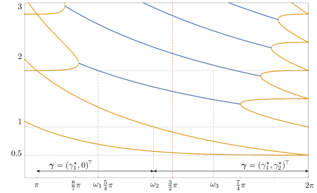
Figure 1: Distribution of the real part of the eigenvalues $\lambda$ with respect to the angle $\omega$ of the re-entrant corner. The blue lines represent complex eigenvalues, the orange ones represent the real eigenvalues. The points of bifurcations, also the point where $\lambda_{2}=1$, have increased multiplicity. In the horizontal axis, $\omega_{i}$, $i=1,2,3$, represent the following cases: $\omega_{1}$ is defined such that $\lambda_{1}+\lambda_{2}=2$, i.e., $\omega_{1}=1.22552...\pi$, $\omega_{2}$ is the unique angle such that $\lambda_{2}=1$, i.e., $\omega_{2}=1.430296...\pi$, and $\omega_{3}$ represents the angle for which $\lambda_{1}+\mathrm{Re}(\lambda_{3})=2$, i.e., $\omega_{3}=1.64941...\pi$. In the plot, there are also included two $\omega-$intervals, $(\pi,\omega_{2})$ and $(\omega_{2},2\pi)$, see Theorem 3.1 and the discussion after.

This is significant, since these roots constrain the regularity of the particular singular functions. The eigenvectors are then, in the polar coordinate-system $(r,\theta)$, log-polynomial functions in $r$ multiplied with smooth functions in $\theta$. Explicitly, for each $\lambda_{i}$ with geometric and algebraic multiplicity $I_{i}$ and $\kappa_{i,j}$, respectively, the singular functions for the velocity and pressure part of the solution are of the form

$$\mathbf{s}^{u}_{i,j,k}=r^{\lambda_{i}}\sum_{l=0}^{k}(\ln r)^{l}\bm{\varphi}^{(i)}_{j,k-l}(\theta),\quad s^{p}_{i,j,k}=r^{\lambda_{i}-1}\sum_{l=0}^{k}(\ln r)^{l}\xi^{(i)}_{j,k-l}(\theta),$$ (6)

$k\in\{0,\kappa_{i,j}-1\}$. Under the assumption that the right-hand side has a higher regularity, i.e., $\mathbf{f}\in L^{2}_{-\alpha}(\Omega)^{2}$ for some $\alpha>1-\lambda$, together with the assumption that $\lambda_{i}$ are simple roots for all $i\in[1,N]$, there holds the following expansion of the solution near the singular point (for simplicity we skip the $j,k$ indices):

$$\mathbf{u}=\sum_{i=1}^{N}c_{i}\ \mathbf{s}^{u}_{i}+\mathbf{U},\qquad p=\sum_{i=1}^{N}c_{i}\ s^{p}_{i}+P,$$ (7)

where $(\mathbf{U},P)\in H^{2}_{-\alpha}(\Omega)^{2}\times H^{1}_{-\alpha}(\Omega)$ is called a smooth remainder. For our needs, we will require a decomposition with two singular functions, i.e., $N=2$. The assumption on simple multiplicity of the eigenvalues is in that case violated only for one angle $\omega_{2}$ in the whole $(\pi,2\pi)$ range.

It is clear from the structure of the singular functions (6) that the integrability and boundedness of the gradients is limited which results in a reduced regularity of the solution in domains with re-entrant corners. On the other hand, the special polynomial structure in $r$ of the singularities can be well-handled in the framework of the Kondratev-type Sobolev spaces. Hence, one can obtain a generalized regularity result

$$\|\mathbf{u}\|_{2,\beta}+\|p\|_{1,\beta}\lesssim\|\mathbf{f}\|_{0,\beta},$$ (8)

see, e.g., [21]. The explicit form of the singular parts of the solution $(\mathbf{u},p)$, decomposition (7), a priori bounds following from the structure of the singularities and the smooth remainder, together with regularity (8) are then used in the formulation and the proof of the convergence behavior of the energy-corrected methods, as they are stated below.

3.2 Pollution effect

It is well-known that the influence of the non-convex corners significantly reduces the global accuracy of standard numerical methods. More precisely, standard Galerkin approximations on a sequence of uniformly refined meshes of the Stokes problem are, in general, of the order:

$$\|\nabla(\mathbf{u}-\mathbf{u}_{h})\|_{0}+h^{-\lambda_{1}}\|\mathbf{u}-\mathbf{u}_{h}\|_{0}+\|p-p_{h}\|_{0}=\mathcal{O}(h^{\lambda_{1}}),$$ (9)

cf. [2, 6, 17]. This global effect, which is commonly referred to as pollution cannot be cured by considering different error norms. Also, it is exhibited by all standard (piecewise polynomial) approximations, independently of the approximation order. For the illustration of the pollution effect, we present the errors and convergence rates for the stable Taylor–Hood element in Tab. 1, where we compare a typical global pollution in the standard approximation with the non-polluted interpolation; cf. also Fig. 2 for some illustration.

$\|\mathbf{u}-\mathbf{u}_{h}\|_{0}$	eoc	$\|p-p_{h}\|_{0}$	eoc	$\|\mathbf{u}-\mathbf{u}_{h}\|_{0,\alpha}$	eoc	$\|p-p_{h}\|_{0,\alpha}$	eoc
6.24297e–02	–	3.76799e–01	–	2.94081e–02	–	4.73148e–01	–
3.03536e–02	1.04	2.00709e–01	0.91	9.38624e–03	1.65	1.72502e–01	1.46
1.20753e–02	1.33	1.27266e–01	0.66	3.21263e–03	1.55	7.58580e–02	1.19
4.90503e–03	1.30	8.06119e–02	0.66	1.36660e–03	1.23	3.50865e–02	1.11
2.06841e–03	1.25	5.23079e–02	0.62	6.20441e–04	1.14	1.65028e–02	1.09
9.04139e–04	1.19	3.47209e–02	0.59	2.88024e–04	1.11	7.78711e–03	1.08
4.06348e–04	1.15	2.33942e–02	0.57	1.34837e–04	1.09	3.67251e–03	1.08

Table 1: Errors and the convergence rates of the standard Galerkin approximation in standard and weighted norms ($\alpha=1-\lambda_{1}$) in the case of the L-shape domain (see Fig. 3 third from left) using the (higher-order) Taylor–Hood element, computed for an exact solution $(\mathbf{s}^{u}_{1}+\mathbf{s}^{u}_{2},s^{p}_{1}+s^{p}_{2}-|\Omega|^{-1}\langle s^{p}_{1}+s^{p}_{2},1\rangle_{\Omega})$. Estimated convergence rates of the errors in standard norms are for the velocity: $2\lambda_{1}=1.09$ and the pressure: $\lambda_{1}=0.54$.

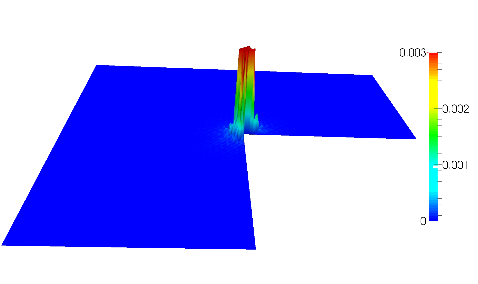
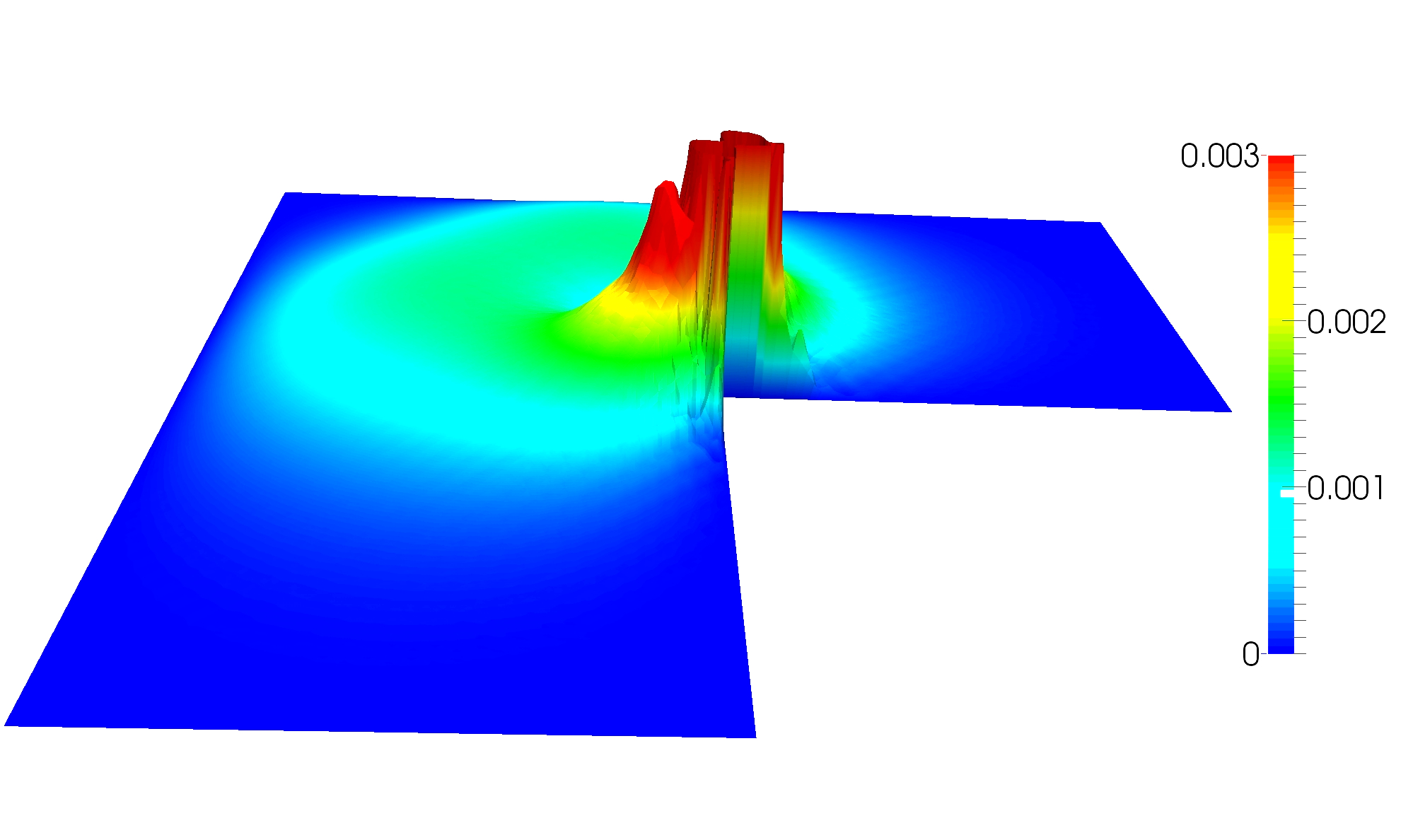
Figure 2: Illustration of the global propagation of the pollution in a L-shape domain with exact solution: $(\mathbf{s}^{u}_{1},s^{p}_{1}-|\Omega|^{-1}\langle s^{p}_{1},1\rangle_{\Omega})$ for the Taylor–Hood element; left: non-polluted $|\mathbf{s}^{u}_{1}-I_{h}^{2}\mathbf{s}^{u}_{1}|$, right: $|\mathbf{s}^{u}_{1}-\mathbf{s}^{u}_{1,h}|$ on level $\ell=4$.

3.3 The energy-corrected scheme

Let us now focus on the a priori energy-modification for the stabilized scheme. We closely follow the theory given in [24], thus it serves as a reference for additional information or rigorous proofs for the presented statements. In view of this approach, we define for a given correction vector $\bm{\gamma}=(\gamma_{1},\gamma_{2})^{\top}$, at this point not closely specified, a mesh-dependent bilinear form $a_{h}(\cdot,\cdot)$ for $\mathbf{v}_{h},\mathbf{w}_{h}\in\mathbf{V}_{h}$ by:

$$a_{h}(\mathbf{w}_{h},\mathbf{v}_{h}) \coloneqq a(\mathbf{w}_{h},\mathbf{v}_{h})-d_{h}(\mathbf{w}_{h},\mathbf{v}_{h})$$ (10)

$$=\sum_{T\in\mathcal{T}_{h}\setminus(\mathcal{L}^{1}_{h}\cup\mathcal{L}^{2}_{h})}a_{T}(\mathbf{w}_{h},\mathbf{v}_{h})+\sum_{i=1,2}(1-\gamma_{i})\sum_{T\in\mathcal{L}^{i}_{h}}a_{T}(\mathbf{w}_{h},\mathbf{v}_{h}),$$

where $a_{T}(\mathbf{w}_{h},\mathbf{v}_{h})\coloneqq\int_{T}\nabla\mathbf{w}_{h}:\nabla\mathbf{v}_{h}\,dx$, $\mathcal{L}_{h}^{i}$ are defined as sets of elements which are in the $i-$th element layer around the singular point, and a stabilization term

$$c_{h}(q_{h},z_{h}) \coloneqq\sum_{T\in\mathcal{T}_{h}\setminus(\mathcal{L}^{1}_{h}\cup\mathcal{L}^{2}_{h})}c_{T}(q_{h},z_{h})+\sum_{i=1,2}\frac{1}{1-\gamma_{i}}\sum_{T\in\mathcal{L}^{i}_{h}}c_{T}(q_{h},z_{h}).$$ (11)

The stabilized energy-corrected finite element approximation to (2) is then formulated for the bilinear forms $a_{h}(\cdot,\cdot)$ and $c_{h}(\cdot,\cdot)$. Namely, we find $({\mathbf{u}}^{\text{m}}_{h},{p}^{\text{m}}_{h})\in\mathbf{V}_{h}\times Q_{h}$ such that

$$a_{h}({\mathbf{u}}^{\text{m}}_{h},\mathbf{v}_{h}) +b(\mathbf{v}_{h},{p}^{\text{m}}_{h}) =\langle\mathbf{f},\mathbf{v}_{h}\rangle_{\Omega}\qquad \forall\mathbf{v}_{h}\in\mathbf{V}_{h},$$ (12)

$$b({\mathbf{u}}^{\text{m}}_{h},q_{h}) -c_{h}(q_{h},{p}^{\text{m}}_{h}) =\langle f_{\text{st}},q_{h}\rangle_{\Omega} \forall q_{h}\in Q_{h}.$$

By definition (10), and (11), the bilinear forms $a_{h}(\cdot,\cdot)$ and $c_{h}(\cdot,\cdot)$ differ from the ones in the standard stabilized Galerkin approximation only on an $\mathcal{O}(h)-$neighborhood of the singular point.

To measure the impact of the pollution in the $L^{2}-$approximation error, we define the energy defect function (also called pollution function) of the discrete scheme as:

$$g_{h}(\mathbf{u},p)\!\coloneqq a(\mathbf{u}\!-\!{\mathbf{u}}^{\text{m}}_{h},\mathbf{u}\!-\!{\mathbf{u}}^{\text{m}}_{h})\!+\!2b(\mathbf{u}\!-\!{\mathbf{u}}^{\text{m}}_{h},p\!-\!{p}^{\text{m}}_{h})\!-\!d_{h}({\mathbf{u}}^{\text{m}}_{h},{\mathbf{u}}^{\text{m}}_{h})\!-\!c_{h}({p}^{\text{m}}_{h},{p}^{\text{m}}_{h}).$$ (13)

Note, that the pollution function $g_{h}$, as defined in (13), can be expressed in the case of a stable finite element formulation of the incompressible homogeneous Dirichlet problem by:

$$g_{h}(\mathbf{u},p)=a(\mathbf{u},\mathbf{u})-a_{h}({\mathbf{u}}^{\text{m}}_{h},{\mathbf{u}}^{\text{m}}_{h}),$$ (14)

hence the name energy defect function. Also, since the correction will be constructed in such a way that the pollution $g_{h}(\mathbf{u},p)$ is controlled, we speak about energy-corrected finite element schemes.

3.4 Theoretical estimates

Let us present here the main result from [24], which was proven for stable linear approximations (more precisely for the $P_{1}\text{--iso}P_{2}/P_{1}\,$element). If explicitly mentioned, we additionally require a local symmetry in angular direction of the mesh around the re-entrant corner; this condition is denoted by (Sh). Note also, that although the main result is formulated for maximal interior angles in the range of $\omega\in(\pi,\omega_{3})$, the performance of the modification was shown numerically for all $\omega\in(\pi,2\pi)$. One can verify that

$$\|\mathbf{u}-{\mathbf{u}}^{\text{m}}_{h}\|_{0,\alpha}=\mathcal{O}(h^{2})\iff g_{h}(\mathbf{u},p)=\mathcal{O}(h^{2}),$$ (15)

and thus, the following theorem represents the sufficient condition for the optimal convergence. The necessary condition, i.e., the implication from left- to right-hand side, is rather trivial to prove and free of additional assumptions.

Theorem 3.1 (Optimal order convergence)

Let $\omega\in(\pi,\omega_{3})$, $\omega\neq\omega_{2}$, $\mathbf{f}\in L^{2}_{-\alpha}(\Omega)^{2}$ for some $\alpha$ such that $\alpha>1-\lambda_{1}$, let $(\mathbf{V}_{h},Q_{h})$ be a stable pair with $c_{h}(\cdot,\cdot)=0$, and, additionally, let (Sh) hold if $\omega\in[\omega_{1},\omega_{3})$. Moreover, let $\bm{\gamma}\in\mathbb{R}^{2}$ be such that

$$g_{h}(\mathbf{s}^{u}_{i},s^{p}_{i})=\mathcal{O}(h^{2}),\quad\text{ for }\left\{\begin{array}[]{ll}i=1&\text{ if }\omega\in(\pi,\omega_{2}),\\ i=1,2&\text{ if }\omega\in(\omega_{2},\omega_{3}),\end{array}\right.$$ (18)

where $\omega_{1}$, $\omega_{2}$ and $\omega_{3}$ are defined as in Fig 1. Then, the modified Galerkin approximation $({\mathbf{u}}^{\text{m}}_{h},{p}^{\text{m}}_{h})\in\mathbf{V}_{h}\times Q_{h}$ converges optimally, i.e.,

$$\|\mathbf{u}-{\mathbf{u}}^{\text{m}}_{h}\|_{0,\alpha}\lesssim h^{2}\|\mathbf{f}\|_{0,-\alpha},\quad\text{and}\quad\|\mathbf{u}-{\mathbf{u}}^{\text{m}}_{h}\|_{1,\alpha}+\|p-{p}^{\text{m}}_{h}\|_{0,\alpha}\lesssim h\|\mathbf{f}\|_{0,-\alpha}.$$ (19)

First of all, let us describe the assumptions in Theorem 3.1 and the proof-technique, after we shall discuss its generalization to the stabilized case.

At the beginning, we would like to point out here, that $\bm{\gamma}=(\gamma_{1},\gamma_{2})^{\top}\in\mathbb{R}^{2}$ is constrained such that the bilinear forms $a_{h}(\cdot,\cdot)$ and $c_{h}(\cdot,\cdot)$ remain uniformly elliptic and continuous, respectively. This means, since the element layers are disjoint, we actually require $\bm{\gamma}\in\mathcal{B}^{\infty}_{R}(0)$ ($\mathcal{B}^{\infty}_{R}(0)$ being a ball with center in the origin of radius $R<1$ in the $l^{\infty}$ norm). Also, if the first condition of (18) has to be satisfied, i.e., $\omega\in(\pi,\omega_{2})$, we represent the vector $\bm{\gamma}$ for simplicity of notation by $\bm{\gamma}=(\gamma_{1},0)^{\top}.$ In that case, we speak about a single- (or one-) parameter correction modification. Such a case largely inherits the properties of the modification as derived in [12] for the Laplace equation.

The proof of (19) is based on duality arguments and strongly relies on the linearity of the system. Under the assumption, that the right-hand side is of increased regularity, the decomposition (7) can be used on the exact and the approximative solutions (note that the eigenvectors $(\mathbf{s}^{u}_{i},s^{p}_{i})$ are solutions of the Stokes equations themselves), and thus, the pollution in the system can be split into several parts, namely pollution caused by the singular functions, terms corresponding to the smooth remainder and the so-called cross-terms. By standard duality arguments, a uniform inf-sup condition with respect to weighted norms, a priori bounds of the smooth remainder in negatively weighted norms, as introduced by [6], one can show that the terms with smooth remainder are of second order, and thus they do not pollute. The same holds for the cross-terms. However, the proof is technically more involved. More precisely, since the orthogonality of the eigenvectors is, in general, not preserved by the finite element approximations, we have to apply generalized Wahlbin arguments and use the local symmetry condition (Sh) on the mesh. Note here, that the drop of (Sh) for small angles comes from the sufficient regularity of the second singular function, and thus the symmetry arguments do not have to be used. The contribution to the pollution $g_{h}$ by the singular functions cannot be neglected, therefore it is enforced by the modification itself. This exactly reflects the condition (18). As one can see, for angles smaller as $\omega_{2}$ we have for the second singular function: $(\mathbf{s}^{u}_{2},s^{p}_{2})\in H^{2}_{-\varepsilon}(\Omega)^{2}\times H^{1}_{-\varepsilon}(\Omega)$, and thus its pollution is again a priori of second order. This means, it does not have to be corrected. The correction vector $\bm{\gamma}$ is then reduced to a single scalar value, as noted above.

In Theorem 3.1, the weight $\alpha$ is bounded from below which originates in the assumption on the decomposition (7). Note, that also for the results discussed in [24], some additional assumptions on the upper bound are specified. These are mainly for technical reasons, namely restricting the number of singular functions in the decomposition and to ensure the validity of some auxiliary lemmas.

Let us now turn our attention to the extension of Theorem 3.1 to stabilized finite elements. Our approach is motivated by the equivalence of the MINI and a stabilized $P_{1}$–$P_{1}$ element. For that, we define a space of element-wise bubble functions:

$$\mathbf{B}_{h}=\left\{v_{h}\in\mathcal{C}(\overline{\Omega}):v_{h}|_{T}\in\text{span}\{\lambda_{1}^{T},\lambda_{2}^{T},\lambda_{3}^{T}\}\ \forall T\in\mathcal{T}_{h}\right\}^{2},$$ (20)

where $\lambda_{i}^{T}$, $i=1,\dots,3$, denote the barycentric coordinates on the element $T$, see also [2]. The MINI element is then defined via the product $(\mathbf{V}_{h}\oplus\mathbf{B}_{h})\times Q_{h}$. The equivalence of the MINI element and the stabilized one, as defined above, (see [9] for the standard case) holds also for the case of the energy corrected scheme if $c_{h}(\cdot,\cdot)$ is selected appropriately. Namely, we have the following.

Theorem 3.2

Let $\mathbf{f}$ be piecewise constant on each element $T\in\mathcal{T}_{h}$. Then the energy corrected MINI element discretization is equivalent to the energy corrected $P_{1}$–$P_{1}$ discretization with PSPG stabilization (12) where the stabilization parameter $\delta_{T}=\frac{c_{1,T}\,c_{2}}{\alpha_{T}}$. Further, the element-wise constants are determined by

$$\langle\phi_{T},1\rangle_{T}=c_{1,T}\,h_{T}^{2},\qquad\langle\phi_{T},1\rangle_{T}=c_{2}\,|T|,\qquad\langle\nabla\phi_{T},\nabla\phi_{T}\rangle_{T}=\alpha_{T},$$ (21)

where $\phi_{T}\in B_{h}|_{T}$ denotes the bubble function, scaled to a maximal value of one, on each element $T\in\mathcal{T}_{h}$, and $c_{2}=\frac{9}{20}$.

Proof.

Let us consider the energy corrected MINI finite element formulation, and denote the solution by $\mathbf{u}_{h}=\mathbf{u}_{h}^{l}+\mathbf{u}_{h}^{b}$, where $\mathbf{u}_{h}^{l}\in\mathbf{V}_{h}$ and $\mathbf{u}_{h}^{b}=\sum_{T\in\mathcal{T}_{h}}\mathbf{u}_{b,T}\phi_{T}\in\mathbf{B}_{h}$, with $\mathbf{u}_{b,T}\in\mathbb{R}^{2}$. Note that the linear and bubble functions are $A$–orthogonal, i.e., $a(\mathbf{v}_{h}^{l},\phi_{T}\,\mathbf{e}_{i})=0$, $i=1,2$, for all $\mathbf{v}_{h}^{l}\in\mathbf{V}_{h}^{1}$ and $\phi_{T}\in B_{h}$. Let us consider the test function $\mathbf{v}_{h}=\phi_{T}\,\mathbf{e}_{i}$, $i=1,2$, on $T$, then for the first equation of the variational formulation (12), we obtain that

$$(1-\gamma_{T})\,a(\phi_{T}\,\mathbf{u}_{b,T},\phi_{T}\,\mathbf{e}_{i})+b(\phi_{T}\,\mathbf{e}_{i},p_{h})=\langle\mathbf{f},\phi_{T}\,\mathbf{e}_{i}\rangle_{T},$$ (22)

where $\gamma_{T}$ represents the correction parameter on the individual element. Note, $\gamma_{T}=0$ for $T\in\mathcal{T}_{h}\setminus(\mathcal{L}^{1}_{h}\cup\mathcal{L}^{2}_{h})$. Using integration by parts and the fact that $\phi_{T}=0$ on $\partial T$ we have:

$$(\mathbf{u}_{b,T}\cdot\mathbf{e}_{i})(1-\gamma_{T})\langle\nabla\phi_{T},\nabla\phi_{T}\rangle_{T}=\langle\mathbf{f}-\nabla p_{h},\phi_{T}\,\mathbf{e}_{i}\rangle_{T}.$$ (23)

Then, applying the assumption of a piecewise constant $\mathbf{f}$, we get that

$$\mathbf{u}_{b,T}=\frac{1}{\alpha_{T}(1-\gamma_{T})}(\mathbf{f}-\nabla p_{h})|_{T}\,\langle\phi_{T},1\rangle_{T}.$$ (24)

Using this, the bilinear form $b(\cdot,\cdot)$ can be rewritten as:

$$b(\phi_{T}\,\mathbf{u}_{b,T},q_{h}) =(\mathbf{u}_{b,T}\cdot\nabla q_{h})|_{T}\,\langle\phi_{T},1\rangle_{T}=\frac{1}{\alpha_{T}(1-\gamma_{T})}(\mathbf{f}-\nabla p_{h})\cdot\nabla q_{h}|_{T}\,\langle\phi_{T},1\rangle_{T}^{2}$$ (25)

$$=\frac{c_{1,T}\,c_{2}}{\alpha_{T}(1-\gamma_{T})}h_{T}^{2}\langle\mathbf{f}-\nabla p_{h},\nabla q_{h}\rangle_{T},$$ (26)

and thus

$$b(\mathbf{u}_{h}^{l},q_{h})-\sum_{T\in\mathcal{T}_{h}}\frac{1}{1-\gamma_{T}}\delta_{T}\,h_{T}^{2}\langle\nabla p_{h},\nabla q_{h}\rangle_{T}=-\sum_{T\in\mathcal{T}_{h}}\frac{1}{1-\gamma_{T}}\delta_{T}\,h_{T}^{2}\langle\mathbf{f},\nabla q_{h}\rangle_{T},$$ (27)

which corresponds to the PSPG stabilization. ∎

In the case that the computational domain is the L-shape domain with a mesh as depicted by the third one from the left in Fig. 3, the stabilization parameter $\delta_{T}$ is independent of the element and equal to $1/160$. The equivalence from Lemma 3.2 also motivates the extension to other stabilizations, like the Dohrman–Bochev approach [7] or the local projection stabilization [15]. In that case we proceed as before, as we scale the bilinear form $c_{h}(\cdot,\cdot)$ on each element $T\in\mathcal{L}_{h}^{i}$ by the term $(1-\gamma_{i})^{-1}$, for $i=1,2$. We note that this is the inverse scaling of the bilinear form $a_{h}(\cdot,\cdot)$.

3.5 Identification of the correction vector $\bm{\gamma}$

Up to this point, we assumed that the vector $\bm{\gamma}$, chosen such that $g_{h}(\mathbf{u},p)=\mathcal{O}(h^{2})$, is known and exists. If this is the case, then the practical realization into an existing code is straightforward, since it only requires a simple re-scaling of a few local stiffness matrices.

The numerical determination of the unknown $\bm{\gamma}$ was first proposed for the Laplace equation in [12] and theoretically studied in [30]. It is constructed as a limit-vector in a component-wise meaning (or a limit-value), of a sequence $\{\bm{\gamma}_{h}\}_{h>0}$ solving

$$g_{h}(\mathbf{s}^{u}_{i},s^{p}_{i})=\mathbf{0},$$ (28)

for $i=1$ if $\omega\in(\pi,\omega_{2})$, and $i=1,2$ if $\omega\in(\omega_{2},2\pi)$. We understand the notation above in a following functional-setting sense: For each $\bm{\gamma}\in\mathcal{B}_{R}^{\infty}(0)$, the approximation operators $R^{u}:H^{1}_{0}(\Omega)^{2}\rightarrow\mathbf{V}_{h}$ and $R^{p}:L^{2}_{0}(\Omega)\rightarrow Q_{h}$ are considered as functions of $\bm{\gamma}$. Thus, on each computational level, corresponding to a certain $h>0$, we seek a root $\bm{\gamma}_{h}$ of

$$a(\mathbf{s}^{u}_{i},\mathbf{s}^{u}_{i})-\left[a_{h}(R^{u}(\bm{\gamma})\mathbf{s}^{u}_{i},R^{u}(\bm{\gamma})\mathbf{s}^{u}_{i})+c_{h}(R^{p}(\bm{\gamma})s^{p}_{i},R^{p}(\bm{\gamma})s^{p}_{i})\right],$$ (29)

again, $i$ from the same set as above. The existence and uniqueness of the sequence $\{\bm{\gamma}_{h}\}_{h>0}$ can be proved with the help of a fixed point theorem. Scaling arguments and the properties of the energy correction function yield the convergence of $\bm{\gamma}_{h}$, and we denote the asymptotic value by star, i.e., $\bm{\gamma}^{\star}=(\gamma_{1}^{\star},\gamma_{2}^{\star})^{\top}=\left(\lim_{h\rightarrow 0^{+}}\gamma_{1,h},\lim_{h\rightarrow 0^{+}}\gamma_{2,h}\right)^{\!\!\top}$. Then one can show that for $\bm{\gamma}=\bm{\gamma}^{\star}$ the assumption (18) is satisfied. To do so one has to construct a suitable subsequence and exploit the properties of the Jacobi matrix of $g_{h}$. The computation of $\bm{\gamma}^{\star}$ can be accelerated by a combination of a nested hierarchical Newton scheme with some extrapolation technique on a coarse element patch.

We remark that $\bm{\gamma}^{\star}$ depends only on the interior angle $\omega$, on the local element patch and the finite element type, but not on the mesh-size nor on the rest of the mesh/domain. Moreover, many re-entrant corners can be handled by local modifications each of which carrying its own correction parameter.

3.6 Numerical examples

In this section, we consider several numerical examples for the stabilized schemes (2) and (12). The correction parameters are estimated as described above, see Tab. 2, for the initial grids as depicted in Fig. 3, i.e., for the scenarios where $\omega\in\{8/7\pi,5/4\pi,3/2\pi,7/4\pi\}$. We always consider a computational setting for which $(\mathbf{s}^{u}_{1}+\mathbf{s}^{u}_{2},s^{p}_{1}+s^{p}_{2}-|\Omega|^{-1}\langle s^{p}_{1}+s^{p}_{2},1\rangle_{\Omega})$ is the exact solution. Note, that for $\omega=8/7\pi$ we do not require the local symmetry of the mesh at the singular point, for both $\omega=8/7\pi,5/4\pi$ a single-parameter correction can be used, while $\omega=3/2\pi,7/4\pi$ cases require two correction parameters. The last case $\omega=7/4\pi$ represents the extension of the derived theory for angles bigger than $\omega_{3}$. For simplicity, we represent only the results for the velocity, see Tab.3, more precisely, we show the weighted $L^{2}_{\alpha}(\Omega)$ error convergences and their rates.

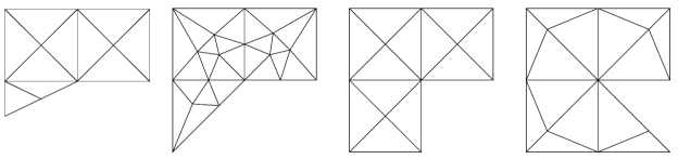
Figure 3: Initial grids for several types of the re-entrant corner, namely $\omega\in\{8/7\pi,5/4\pi,3/2\pi,7/4\pi\}$. All the geometries are bounded by a unit square, particularly $\Omega_{3/2\pi}=(-1,1)^{2}\backslash([0,1]\times[-1,0])$.

$\omega$	$\bm{\gamma}^{\star}$ (single correction)	$\omega$	$\bm{\gamma}^{\star}$ (two corrections)
$8/7\pi$	$(0.011364,0.0)^{\top}$	$3/2\pi$	$(\phantom{-}0.161708,-0.183984)^{\top}$
$5/4\pi$	$(0.017676,0.0)^{\top}$	$7/4\pi$	$(-0.483852,\phantom{-}0.273889)^{\top}$

Table 2: Estimated asymptotic $\bm{\gamma}^{\star}$ for the geometries and local element patches of Fig. 3.

$\omega=8/7\pi$		$\omega=5/4\pi$		$\omega=3/2\pi$		$\omega=7/4\pi$
$\|\mathbf{u}-{\mathbf{u}}^{\text{m}}_{h}\|_{0,\alpha}$	eoc	$\|\mathbf{u}-{\mathbf{u}}^{\text{m}}_{h}\|_{0,\alpha}$	eoc	$\|\mathbf{u}-{\mathbf{u}}^{\text{m}}_{h}\|_{0,\alpha}$	eoc	$\|\mathbf{u}-{\mathbf{u}}^{\text{m}}_{h}\|_{0,\alpha}$	eoc
6.80763e–02	–	6.43853e–02	–	9.87423e–02	–	6.31650e–02	–
2.21098e–02	1.62	2.36951e–02	1.44	3.76712e–02	1.39	1.79778e–02	1.81
6.06479e–03	1.87	6.78762e–03	1.80	1.28515e–02	1.55	4.55198e–03	1.98
1.59057e–03	1.93	1.81517e–03	1.90	3.48892e–03	1.88	1.06693e–03	2.09
4.07657e–04	1.96	4.68415e–04	1.95	8.87484e–04	1.97	2.47722e–04	2.11
1.03206e–04	1.98	1.18907e–04	1.98	2.19857e–04	2.01	5.82728e–05	2.09
2.59642e–05	1.99	2.99543e–05	1.99	5.37256e–05	2.03	1.41046e–05	2.05

Table 3: Errors and the convergence rates of the velocity approximation measured in the weighted norm with $\alpha=1-\lambda_{1}$.

To demonstrate the convergence of the pressure part of the solution, we additionally include Tab.4 for $\omega=3/2\pi$, presenting also the rates and errors in the case of the standard $L^{2}(\Omega)-$norm. For the velocity, we obtain in that case the best approximation order, namely $\lambda_{1}+1=1.54$, instead of the polluted rate $2\lambda_{1}=1.09$, see (9). In the case of the pressure-error, we have increased the weight to $\alpha_{p}=\alpha+0.5$, to restore its superconvergence behavior.

standard norm				weighted norm
$\|\mathbf{u}-{\mathbf{u}}^{\text{m}}_{h}\|_{0}$	eoc	$\|p-{p}^{\text{m}}_{h}\|_{0}$	eoc	$\|\mathbf{u}-{\mathbf{u}}^{\text{m}}_{h}\|_{0,\alpha}$	eoc	$\|p-{p}^{\text{m}}_{h}\|_{0,\alpha_{p}}$	eoc
4.70326e–02	–	7.92268e–01	–	9.87423e–02	–	4.03685e–01	–
3.87065e–02	2.81	4.61252e–01	0.78	3.76712e–02	1.39	2.04358e–01	0.98
1.88110e–02	1.04	2.30692e–01	0.99	1.28515e–02	1.55	5.03504e–02	2.02
7.07091e–03	1.41	1.25586e–01	0.87	3.48892e–03	1.88	1.83549e–02	1.46
2.51514e–03	1.49	6.98617e–02	0.84	8.87484e–04	1.97	6.74790e–03	1.44
8.78492e–04	1.51	3.97820e–02	0.81	2.19857e–04	2.01	2.37574e–03	1.50
3.04097e–04	1.53	2.33040e–02	0.77	5.37256e–05	2.03	8.20768e–04	1.53

Table 4: Convergence results of the velocity and pressure modified approximation measured in the standard and weighted norms, with minimal admissible value $\alpha=1-\lambda_{1}$ and increased weight for pressure $\alpha_{p}=\alpha+0.5$ to restore the superconvergence, in the case of L-shape domain.

Finally, we return to the motivational problem of Fig. 2, i.e., a higher order approximation, and illustrate on the left of Fig. 4 the reduction of the pollution by the energy-corrected scheme, as derived above, for the same computational setting. On the right, we show the solution of an optimal control problem on a domain with multiple (50) re-entrant corners. Here at each corner, the modified scheme can be applied locally with the same correction parameters as for the L-shape domain. Many quantities of interest such as stress intensity factors, eigenvalues or the flow rate can then accurately be determined on uniformly refined meshes, and no mesh grading techniques are required.

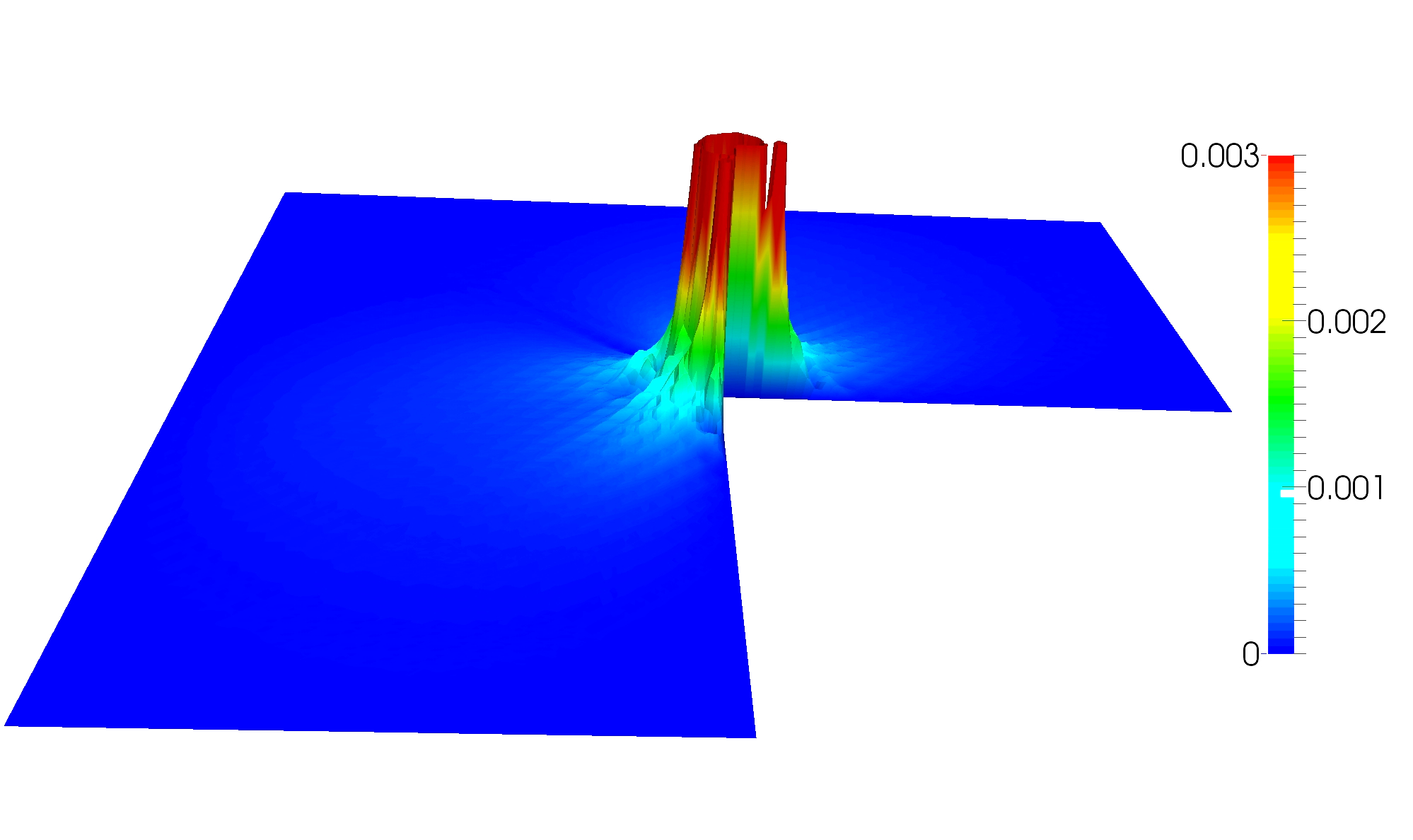
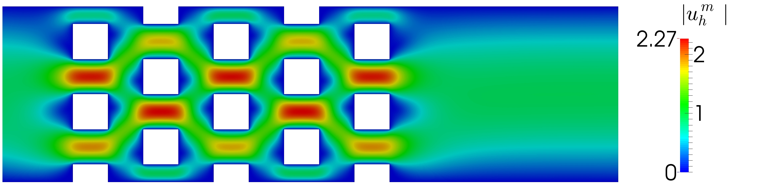
Figure 4: Left: Reduced pollution effect for the modified Taylor–Hood scheme (compare with Fig. 2); Namely we plot $|\mathbf{u}-{\mathbf{u}}^{\text{m}}_{h}|$. Right: Multiple re-entrant corners.

4 Multigrid and fault tolerant algorithms

In this section, we consider the realization of efficient multigrid solvers and fault tolerant algorithms for the Stokes system. Our implementation employs the hierarchical hybrid grids (HHG) finite element framework, see, e.g., [5, 4]. HHG combines the flexibility of unstructured finite element meshes with the performance advantage of structured grids in a block-structured approach. It shows excellent scalability up to the largest supercomputers available [18] and reaches parallel textbook multigrid efficiency [19].

In the following, we denote by $n_{u}={\rm dim}\,\mathbf{V}_{h}$ and $n_{p}={\rm dim}\,Q_{h}$ the number of degrees of freedom for velocity and pressure, respectively. Then, the isomorphisms $\mathbf{u}_{h}\leftrightarrow\mathbf{u}\in\mathbb{R}^{n_{u}}$ and $p_{h}\leftrightarrow\mathbf{p}\in\mathbb{R}^{n_{p}}$ are obvious. The discrete variational formulation (2) is then equivalent to the linear system

$$\mathcal{K}\begin{pmatrix}\mathbf{u}\\ \mathbf{p}\end{pmatrix}:=\begin{pmatrix}A&B^{\top}\\ B&-C\end{pmatrix}\begin{pmatrix}\mathbf{u}\\ \mathbf{p}\end{pmatrix}=\begin{pmatrix}\mathbf{f}\phantom{s}\\ \mathbf{f}_{\text{st}}\end{pmatrix},$$ (30)

where $\mathcal{K}\in\mathbb{R}^{(n_{u}+n_{p})\times(n_{u}+n_{p})}$. The matrix A has a $3\times 3$ diagonal block structure consisting of three discrete representations of the Laplace operator.

In the following, we describe a multigrid solver for this structure and a multigrid based fault tolerant solution strategy.

4.1 Multigrid solver

Iterative methods for solving the saddle point system can e.g. be constructed based on the pressure Schur complement (SCG) or on a preconditioned MINRES method, see, e.g., [13, 32].

Here, we consider an all-at-once multigrid method for the linear system (30). The key point in a multigrid method for the entire saddle point problem is the construction of a suitable smoother. We shall consider Uzawa type smoothers, see, e.g., [3, 31, 34]. This idea is based on a preconditioned Richardson method, where in iteration $k+1$ the system for $(\mathbf{u}_{k+1},\mathbf{p}_{k+1})$ must be solved

$$\hat{\mathcal{K}}\begin{pmatrix}\mathbf{u}_{k+1}-\mathbf{u}_{k}\\ \mathbf{p}_{k+1}-\mathbf{p}_{k}\end{pmatrix}=\begin{pmatrix}\mathbf{f}\phantom{s}\\ \mathbf{f}_{\text{st}}\end{pmatrix}-\mathcal{K}\begin{pmatrix}\mathbf{u}_{k}\\ \mathbf{p}_{k}\end{pmatrix}.$$ (31)

Here $\mathcal{K}$ denotes the system matrix (30) of the Stokes equations and $\hat{\mathcal{K}}$ an appropriate preconditioner. The corresponding iteration matrix is then given by $\mathcal{M}\coloneqq I-\hat{\mathcal{K}}^{-1}\mathcal{K}$. We note that for the convergence of (31), the analysis of $\mathcal{M}^{k}$ is needed, while for showing a qualitative smoothing property, the matrix polynomial $(I-\mathcal{M})\mathcal{M}^{k}$ must be analyzed [25, 31]. Approaches towards a full quantitative multigrid analysis based on Fourier techniques are presented in [16]. In general several choices for $\hat{\mathcal{K}}$ are available, we restrict ourselves to

$$\hat{\mathcal{K}}\coloneqq\begin{pmatrix}\hat{A}&0\\ B&-\hat{S}\end{pmatrix},$$

where $\hat{A}$ and $\hat{S}$ are suitable smoothers for the upper left block $A$ and the pressure Schur complement $S\coloneqq BA^{-1}B^{\top}+C$, respectively. The application of $\hat{\mathcal{K}}$ results in the algorithm of the inexact Uzawa method, where we smooth the velocity part in a first step and in a second step the pressure, i.e.

$$1.\quad\mathbf{u}_{k+1}=\mathbf{u}_{k}+\hat{A}^{-1}(\mathbf{f}-A\mathbf{u}_{k}-B^{\top}\mathbf{p}_{k}),$$

$$2.\quad\mathbf{p}_{k+1}=\mathbf{p}_{k}+\hat{S}^{-1}(B\mathbf{u}_{k+1}-C\mathbf{p}_{k}-\mathbf{f}_{\text{st}}).$$

Other variants of Uzawa-type multigrid methods, such as the symmetric version, are for instance considered in [31]. In each smoothing step, we consider for the velocity smoother $\hat{A}$, a combination of a forward and backward communication reducing variant of a Gauß–Seidel scheme with an additional row-wise red-black coloring in each of the parallel distributed subdomains. Within the parallel data structures this results in a combined block Jacobi- and symmetric Gauß–Seidel updating scheme. For the pressure, we use a SOR applied on the matrix $C$ with the under-relaxation parameter $\omega=0.3$. These smoothers are then applied within a multigrid V-cycle, where we vary the number of smoothing steps from 3 pre- and 3 post smoothing steps on the finest level to 5 pre- and 5 post-smoothing steps on coarser levels. This leads to a good efficiency.

As a solver on the coarsest level, several choices are available. This includes parallel sparse direct solvers, such as PARDISO [22], or algebraic multigrid methods, such as hypre [14]. For this performance study, we avoid the dependency on external libraries and employ a preconditioned MINRES as coarse-grid solver for the saddle point system (30). The preconditioner consists of CG and a lumped mass matrix $M$. The relative accuracy is set to $\varepsilon=5\cdot 10^{-3}$.

Numerical examples

In the following, we present several numerical examples, illustrating the robustness and scalability of our solver. As a computational domain, we consider the unit cube $\Omega=(0,1)^{3}$ with an initial mesh $\mathcal{T}_{-2}$ consisting of 6 tetrahedra. The coarse grid $\mathcal{T}_{0}$ is a twice refined initial grid, where each tetrahedron is decomposed into 8 new ones. The right-hand side $\mathbf{f}=\mathbf{0}$ and for the initial guess $\mathbf{x}_{0}=(\mathbf{u}_{0},\mathbf{p}_{0})^{\top}$, we distinguish between velocity and pressure part. Here $\mathbf{u}_{0}$ is a random vector with values in $[0,1]$, while the initial random pressure $\mathbf{p}_{0}$ is scaled by $h^{-1}$, i.e.,  with values in $[0,h^{-1}]$. This is important in order to represent a less regular pressure, since the velocity is generally considered as a $H^{1}(\Omega)$ and the pressure as a $L^{2}(\Omega)$ function. Unless further specified, we use the relative reduction of the residual by $\varepsilon=10^{-8}$ as a stopping criteria. Numerical examples are performed on a low cost desktop machine, an Intel Xeon CPU E2-1226 v3, 3.30GHz and 32 GB shared memory for serial computations and on JUQUEEN (Jülich Supercomputing Center, Germany) for massively parallel computations.

SCG Uzawa $L$ DoF iter TtS [s] iter TtS [s] 2 $1.4\cdot 10^{4\,}$ 26 0.11 9 0.08 3 $1.2\cdot 10^{5\,}$ 28 0.56 8 0.29 4 $1.0\cdot 10^{6\,}$ 28 3.33 8 1.79 5 $8.2\cdot 10^{6\,}$ 28 24.28 8 12.70 6 $6.6\cdot 10^{7\,}$ 31 205.84 8 95.85 7 $5.3\cdot 10^{8\,}$ out of mem. 8 730.77

Table 5: Iteration numbers and time-to-solution (TtS) (left) and number of operator evaluations for $L=6$ (right) for the serial case.

In Tab. 5, we present results for several refinement levels $L$ and a fixed coarse grid $\mathcal{T}_{0}$. We observe that the multigrid convergence rates are independent of the mesh size, as expected. We also include results for the Schur complement CG method [18], where we observe that the Uzawa multigrid solver is typically a factor of two faster and is more memory efficient. The number of operator evaluations for the individual blocks, which are computed by $n_{\text{op}}=\sum_{\ell=0}^{L}8^{\ell-L}n_{\text{op},\ell}$, where $n_{\text{op},\ell}\in\mathbb{N}$ denotes the number of operator evaluations on level $\ell$, are presented too. These numbers are also reflected by the time to solution of the individual solvers.

Nodes	Threads	DoF	iter	TtS [s]	T${}_{\!w}$ [s]	T${}_{\!c}$[%]
1	24	$6.6\cdot 10^{7\ }$	7 (1)	65.71	58.80	10.5
6	192	$5.3\cdot 10^{8\ }$	7 (3)	80.42	64.40	19.9
48	1 536	$4.3\cdot 10^{9\ }$	7 (5)	85.28	65.03	23.7
384	12 288	$3.4\cdot 10^{10}$	7 (10)	93.19	64.96	30.3
3 072	98 304	$2.7\cdot 10^{11}$	7 (20)	114.36	66.08	42.2
24 576	786 432	$2.2\cdot 10^{12}$	8 (40)	177.69	78.24	56.0

Table 6: Weak scaling result times for the Uzawa multigrid method; number of iterations, including number of iterations of the preconditioner on the coarse grid, time-to-solution (TtS), TtS without the time spent by the coarse grid iterations (T${}_{\!w}$), and the time spent by the coarse grid in percents (T${}_{\!c}$).

Scaling results are present for up to $786\,432$ threads and more than $10^{12}$ degrees of freedom (DoF). We use 32 threads per node and 6 tetrahedra in the initial mesh per thread. The finest computational level is obtained by a 7 times refined initial mesh. Excellent scalability for the multilevel part of the algorithm is achieved, see Tab. 6. We point out that the coarse grid solver in these examples considered as a stand-alone solver lacks optimal complexity. However, even for the largest example with more than $10^{12}$ DoF it still requires less than 60% of the overall time.

4.2 Fault tolerant algorithms

In the future era of exa-scale computing systems, highly scalable implementations will execute up to billions of parallel threads on millions of compute nodes. In this scenario, fault tolerance will become a necessary property of hardware, software and algorithms. Nevertheless, nowadays commonly used redundancy approaches, e.g., check-pointing, will be too costly, due to the memory and energy consumption. Our approach, on the other hand, incorporates the resilience strategy directly into the multigrid solver, and thus does not require additional memory.

In [23], we introduce a methodology and data-structure to efficiently recover lost data due to a processor crash (hard fault) when solving elliptic PDEs with multigrid algorithms. We consider a fault model where a processor stores the mesh data of a subdomain including all its refined levels in the multigrid hierarchy. Therefore, when a processor crashes all data is lost in the faulty domain $\Omega_{F}\subset\Omega$. The healthy domain $\Omega_{H}\subset\Omega$ is unaffected by the fault, and data in this domain remains available. Further, we denote by $\Gamma\coloneqq\partial\Omega_{F}\cap\partial\Omega_{H}$ the interface. The nodes associated with $\Gamma$ are used to communicate between neighboring processors by introducing ghost copies that redundantly exist on different processors. Therefore, a complete recovery of these nodes is possible without additional redundant storage.

In order to recover the lost nodal values $(\mathbf{u}_{F},\mathbf{p}_{F})$ in $\Omega_{F}$, we propose to solve a local subproblem in $\Omega_{F}$ of (1) with Dirichlet boundary conditions on $\Gamma$ for velocity and pressure, respectively. To guarantee that the local system is uniformly well-posed, we formally include a compatibility condition obtained from the normal components of the velocity. If the local solution in $\Omega_{F}$ is computed while the global process is halted, then this is a local recovery strategy. For a first analysis, we assume that the local recovery is free of cost, i.e., that it can be executed in zero time.

In [23] this local strategy is extended to become a global recovery strategy. To this end, the solution algorithm proceeds asynchronously in the faulty and the healthy domain such that no process remains idle. Temporarily, the two subdomains are decoupled at the interface $\Gamma$, and the recovery process is accelerated by delegating more compute resources to it. This acceleration is termed the superman strategy. Once the recovery has proceeded far enough and has caught up with the regular solution process, both subdomains are re-coupled and the regular global iteration is resumed. These approaches result in a time- and energy-efficient recovery of the lost data.

Numerical examples

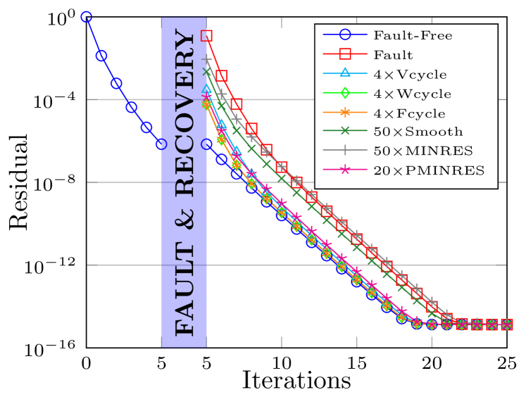
	DN Strategy $\eta_{\text{super}}=4$
Size	${n_{H}}=0$	$2$	$3$	$4$
$769^{3}$	19.21	0.05	-0.38	4.22
$1\,281^{3}$	21.27	-0.15	-0.68	3.95
$2\,305^{3}$	18.50	-0.33	-0.87	3.76
$4\,353^{3}$	19.74	2.58	4.61	9.24

Figure 5: Left: Convergence of the relative residual for different local recovery strategies, Right: Global recovery in terms of a domain partitioning concept with over-balancing by a factor of $\eta_{\text{super}}=4$ in the case of the Laplace operator.

In Fig. 5 (left), we consider a test scenario in $\Omega=(0,1)^{3}$ in which we continuously apply multigrid V(3,3)-cycles of the Uzawa multigrid method introduced in Sect. 4.1. In total 23 iterations are needed to reach the round-off limit of $10^{-15}$. During the iteration, a fault is provoked after 5 iterations. This affects 2.1% of the pressure and velocity unknowns. We continue with global solves after the recovery by solving the local auxiliary problem iteratively in $\Omega_{F}$. As approximate subdomain solvers we compare the fine grid Uzawa-smoother, the minimal residual method, the block-diagonal preconditioned MINRES (PMINRES) method and V, F, W-cycles in the variable smoothing variant from Sect. 4.1. For the block-preconditioner in case of PMINRES a standard V-cycle and a lumped mass-matrix $M$ are used. Fig. 5 (left) displays also the cases in which no fault appears (fault-free) and when no recovery is performed after the fault.

After the fault, we observe that the residual jumps up and when no recovery is performed, the iteration must start almost from the beginning. A higher pre-asymptotic convergence rate after the fault helps to catch up, so that only four additional iterations are required. This delay can be further reduced by a local recovery computation, but only local multigrid cycles are found to be efficient recovery methods. Four local recovery multigrid cycles are sufficient such that the round-off limit is reached with the same number of iterations as in the fault-free case. The other recovery methods either yield no significant improvement or too many recovery iterations would be required.

The table on the right of Fig. 5 summarizes the performance of the global recovery in terms of the time delay (in seconds compute time) as compared to an iteration without faults. The tests are performed for a large Laplace problem discretized with up to almost $10^{11}$ unknowns. The undisturbed solution takes 50.49 seconds with 14 743 cores on JUQUEEN. Two faults are provoked, one after 5 V-cycles, one after 9. Both faults are treated with both the global recovery strategy and a local superman process that is $\eta_{\text{super}}=4$ times as fast a a regular processor. Faulty and healthy domain remain decoupled for ${n_{H}}$ cycles with the Dirichlet-Neumann strategy, i.e., solving a Dirichlet problem on $\Omega_{F}$ and a Neumann problem on $\Omega_{H}$, then the regular iteration is resumed. The case ${n_{H}}=0$ corresponds to performing no recovery at all and leads to a delay of about 20 seconds. By the superman recovery and global re-coupling after ${n_{H}}=2$ cycles, the delay can be reduced to just a few seconds. In some cases the fault-affected computation is even faster than the regular one, as indicated by negative time delays in the table.

5 A posteriori mass correction

A common problem of continuous pressure finite element methods, such as the stabilized scheme considered in this work, is that they do not preserve the physical concept of mass-conservation in a local sense. Although the discrete solution $\mathbf{u}_{h}\in\mathbf{V}_{h}$ satisfies a weak form of the mass-balance equation, it can, in general, not be considered as element-wise mass conservative. Due to the lack of element-piecewise constants in the pressure space, we cannot expect a property of the form

$$\int_{\partial T}\mathbf{u}_{h}\cdot\mathbf{n}\,{\rm d}s=0,\quad T\in\mathcal{T}_{h},$$

to hold, which is a crucial prerequisite to enable an element-by-element post-processing of the discrete solution to obtain strongly divergence-free velocities. However, we will demonstrate how a local conservation property can be obtained also for continuous pressure interpolations. For this we need to change the viewpoint which requires some additional notation that is introduced next.

5.1 Dual mesh

Based on the triangulation $\mathcal{T}_{h}$, which we refer to $\mathcal{T}_{h}$ as the primal mesh, we construct a dual mesh as it is often done for finite-volume methods. To be precise, let $\mathcal{T}_{i}\subseteq\mathcal{T}_{h}$ denote the nodal patch associated with the vertex $\mathbf{x}_{i}$, $i=1,\dots,N$, of the primal mesh, and let $\lambda^{T}_{i}(\mathbf{x})$ denote the barycentric coordinate of $\mathbf{x}\in\mathbb{R}^{d}$ with respect to the vertex $\mathbf{x}_{i}$ belonging to any element $T\in\mathcal{T}_{i}$. We define

$$B_{i}^{T}:=\{\mathbf{x}\,:\,\lambda_{i}^{T}(\mathbf{x})\geq\lambda_{j}^{T}(\mathbf{x}),~{}i\neq j\},$$

and we set $B_{i}:=\bigcup_{T\in\mathcal{T}_{i}}B_{i}^{T}.$ This construction results in a partition of $\Omega$ into $d$-polytopes $B_{i}$ which we shall refer to as the set $\mathcal{B}_{h}:=\{B_{i},i=1,\dots,N\}$ of control volumes. For an illustration of typical control volumes in $d=2,3$ dimensions, we refer to Fig. 6.

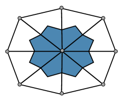
Figure 6: Illustration of a nodal patch $\mathcal{T}_{i}$ around a vertex $\mathbf{x}_{i}$ with the associated dual control volume $B_{i}$ (shaded) for $d=2$ (left) and $d=3$ (right).

The boundary $\partial B_{i}$ of every such volume $B_{i}$ can be decomposed into the set of internal control facets $\gamma_{ij}^{T}\coloneqq\partial B_{i}\cap\partial B_{j}\cap T:B_{j}\neq B_{i}$ and boundary facets $\gamma_{i\partial}^{T}\coloneqq\partial\Omega\cap\partial B_{i}\cap\partial T$, where $B_{i}$ and $B_{j}\in\mathcal{B}_{h}$ are the control volumes defined with respect to the two vertices $\mathbf{x}_{i}$ and $\mathbf{x}_{j}$, which are both end points of an edge of some $T\in\mathcal{T}_{h}$. With each $\gamma_{ij}^{T}$ we associate a unique normal $\mathbf{n}_{ij}^{T}$ oriented from $B_{i}^{T}$ towards $B_{j}^{T}$. We note that the two faces $\gamma_{ij}^{T}$ and $\gamma_{ji}^{T}$ are geometrically the same but have a differently oriented normal. We are now prepared to discuss mass conservation properties on the dual mesh.

5.2 Corrected mass flux

In the following, we consider a wider class of continuous-pressure discretization schemes. After we state the main result, we discuss simplifications that are possible if the choice of the finite-element spaces is restricted to stabilized linear equal-order elements as discussed in this work. For the moment let us put the previous definitions aside and assume that $\mathbf{V}_{h}\times Q_{h}$ is a continuous mixed finite element space which may be stable or unstable. For unstable choices, we require that appropriate stabilization terms are added to the variational form such that a unique discrete solution exists.

Given a finite element solution $(\mathbf{u}_{h},p_{h})\in\mathbf{V}_{h}\times Q_{h}$, we define a mass flux defect

$$\kappa_{ij}^{T}(\mathbf{u}_{h},p_{h}):=\frac{1}{(d+1)|\gamma_{ij}^{T}|}\big{(}\mathcal{R}_{i}^{T}(\mathbf{u}_{h},p_{h})-\mathcal{R}_{j}^{T}(\mathbf{u}_{h},p_{h})\big{)},$$ (32)

where the local residual fluxes $\mathcal{R}_{i}^{T}$ are defined as

$$\mathcal{R}_{i}^{T}(\mathbf{u}_{h},p_{h}):=\int_{B_{i}^{T}}\mathop{\mathrm{div}}\nolimits\mathbf{u}_{h}\,{\rm d}x-\int_{T}\mathop{\mathrm{div}}\nolimits\mathbf{u}_{h}\,\phi_{i}\,{\rm d}x-c_{T}(p_{h},\phi_{i})-\langle f_{\text{st}},\phi_{i}\rangle_{T},$$

with $\phi_{i}\in Q_{h}$ denoting the linear nodal shape function associated with the local vertex $i$ of element $T\in\mathcal{T}_{h}$. Finally, we define the corrected mass flux $j(\mathbf{u}_{h},p_{h})$ which is oriented and defined facet-wise as

$$j(\mathbf{u}_{h},p_{h})|_{\gamma_{ij}^{T}}:=\mathbf{u}_{h}|_{\gamma_{ij}^{T}}\cdot\mathbf{n}_{ij}^{T}-\kappa_{ij}^{T}(\mathbf{u}_{h},p_{h}).$$ (33)

Given these preparations, we formulate our main observation, which is the conservation of the corrected fluxes over the boundary of a dual control volume.

Theorem 5.1

Let $(\mathbf{u}_{h},p_{h})\in\mathbf{V}_{h}\times Q_{h}$ denote the solution of the discrete Stokes problem and assume that $c_{T}(\cdot,1)+\langle f_{\text{st}},1\rangle_{T}=0$ for every $T\in\mathcal{T}_{h}$. Then the corrected mass-flux $j(\mathbf{u}_{h},p_{h})$ is locally conservative, i.e.,

$$\int_{\partial B}j(\mathbf{u}_{h},p_{h})\,{\rm d}s=0,\qquad B\in\mathcal{B}_{h}.$$

The proof is based on summation arguments and the weak mass-conservation property of the discrete solution, see [20, Theorem 3.2].

Revisiting the construction of the mass-correction, we observe that for a stable pairing without additional stabilization terms (such as the classical Taylor-Hood element), the defect $\kappa_{ij}^{T}(\mathbf{u}_{h},p_{h})$ obviously does not depend on $p_{h}$, while for stabilized equal-order linear elements the correction does not depend on $\mathbf{u}_{h}$ since we find by a simple integration that the divergence terms cancel inside each element. The remaining terms can often be considerably simplified, e.g., for the stabilized discretization we consider in this paper, we find that the flux correction assumes the simple form

$$\kappa^{T}_{ij}(p_{h})=\delta_{T}h_{T}^{2}\nabla p_{h}|_{T}\cdot\mathbf{n}_{ij}^{T}.$$ (34)

which can be straightforwardly evaluated.

Given a locally conservative mass-flux on the dual mesh, we could next solve local equilibration problems to obtain local fluxes also with respect to the primal mesh. This allows the lifting of the correction into $H(\mathrm{div})$-conforming finite element spaces and thereby allows us to define a strongly mass-conservative velocity solution with the same order of convergence as the original finite element solution without post-processing. Details are outlined in [20].

However, when coupling the equal-order linear stabilized scheme to transport problems, we can even circumvent the reconstruction step by directly solving the transport equations on the dual mesh in a finite volume fashion, using the corrected mass fluxes for advection.

5.3 Conservative coupling to transport equations

In many applications non-isothermal models (e.g., mantle convection) or reactive models (e.g., the simulation of thrombus formation in the human blood-stream) are considered. What these models have in common is that we couple fluid flow in the form of (1) to a (set of) transport equation(s) of the form:

$$\partial_{t}\vartheta+\mathop{\mathrm{div}}\nolimits(\vartheta\mathbf{u}-\varepsilon\nabla\vartheta)=0\qquad\text{ in }\Omega\times(0,t_{\rm end}],$$ (35)

for some simulation end time $t_{\rm end}>0$, where $\vartheta$ denotes the transported quantity, $\varepsilon>0$ plays the role of a conductivity, and $\mathbf{u}$ is an often dominant advective velocity field that typically results from a flow simulation. To make the problem well-posed, we consider an initial temperature field $\vartheta(t=0)=\vartheta^{0}$ and homogeneous Neumann boundary conditions $\varepsilon\nabla\vartheta\cdot\mathbf{n}=0$ on the whole boundary $\partial\Omega$ of the computational domain, where $\mathbf{n}$ denotes an outward-pointing unit-normal vector. This is done only for simplicity of the exposition and as we will see in the numerical examples the extension to other types of boundary conditions is possible.

Of course, in non-isothermal models the flow-properties such as the forcing or the viscosity may again depend non-linearly on $\vartheta$. However, for simplicity we shall consider only a one-way coupling between flow and transport here. For more general models with full non-isothermal coupling we refer to our recent work [33].

Our aim is to complement the equal-order linear stabilized scheme with a finite-volume solver that associates nodal degrees of freedom with unknown coefficients. Therefore, we define the following space on the barycentric dual mesh:

$$R_{h}:=\{r_{h}\in L^{2}(\Omega)\,:\,r_{h}|_{B}\in P_{0}(B),\,B\in\mathcal{B}_{h}\},$$

We note that due to the fact that $\mathrm{dim}\,R_{h}=\mathrm{dim}\,V_{h}=n_{p}$, we can define a natural bijection between these two spaces. More precisely, given the nodal basis $\phi_{i}$ of $V_{h}$ and the piecewise constant basis $\chi_{i}$ of $R_{h}$, we can define the natural transfer operators $\pi_{h}:\sum_{i=1}^{n_{p}}q_{i}\chi_{i}\to\sum\noindent_{i=1}^{n_{p}}q_{i}\phi_{i}$, and $\overline{\pi}_{h}:\sum\noindent_{i=1}^{n_{p}}q_{i}\phi_{i}\to\sum\noindent_{i=1}^{n_{p}}q_{i}\chi_{i}$ which by construction satisfy the property $\pi_{h}\overline{\pi}_{h}=\overline{\pi}_{h}\pi_{h}=\text{id}$.

Based on the discrete velocity solution of (2) or (12), the transport equation for the temperature can be then advanced by an upwind finite-volume scheme which we state in form of a Petrov-Galerkin method: given $(\mathbf{u}_{h}^{n},p_{h}^{n})\in\mathbf{V}_{h}\times Q_{h}$ and $\vartheta_{h}^{n}\in V_{h}$, find $\vartheta_{h}^{n+1}\in V_{h}$ such that

$$\sum_{B_{i}\in\mathcal{B}_{h}}\int_{B_{i}}\overline{\pi}_{h}\vartheta_{h}^{n+1}\,r_{h}\,{\rm d}x=\sum_{B_{i}\in\mathcal{B}_{h}}\int_{B_{i}}\vartheta_{h}^{n}\,r_{h}\,{\rm d}x-\Delta{t}_{n}\,\mathcal{A}(\vartheta_{h}^{n},r_{h}),$$ (36)

for all $r_{h}\in R_{h}$, where the use of $\overline{\pi}_{h}$ introduces a mass-lumping, and we set the bilinear form

$$\mathcal{A}(\vartheta_{h}^{n},r_{h}):=\sum_{B_{i}\in\mathcal{B}_{h}}\int_{\partial B_{i}\backslash\partial\Omega}\left({\rm j}(\mathbf{u}_{h}^{n},p_{h}^{n})\,\langle\vartheta_{h}^{n}\rangle_{\rm up}-\varepsilon\nabla\vartheta_{h}^{n}\cdot\mathbf{n}_{i}\right)\,r_{h}\,{\rm d}s,$$

where $\mathbf{n}_{i}$ is the unit normal vector pointing outward of $B_{i}$. To ensure stability, we use an up-winding, namely

$$\langle\vartheta_{h}^{n}\rangle_{\rm up}|_{\partial B_{i}\cap\gamma_{ij}^{T}}:=\begin{cases}\vartheta_{h}^{n}|_{B_{i}}&\text{if }{\rm J}_{ij}^{T}\geq 0\\ \vartheta_{h}^{n}|_{B_{j}}&\text{if }{\rm J}_{ij}^{T}\leq 0\\ \end{cases},\qquad i\neq j,$$

where we define the net flux ${\rm J}_{ij}^{T}:=\int_{\gamma_{ij}^{T}}{\rm j}(\mathbf{u}_{h}^{n},p_{h}^{n})|_{\partial B_{i}}\,{\rm d}s$ based on the locally conservative facet flux function

$${\rm j}(\mathbf{u}_{h}^{n},p_{h}^{n})|_{\partial B_{i}}:=(\mathbf{u}_{h}^{n}-\delta_{T}h_{T}^{2}\nabla p_{h}^{n})|_{\partial B_{i}}\cdot\mathbf{n}_{i}.$$ (37)

The distinctive feature of this method is that it can be implemented with minimal overhead, using only nodal data structures on semi-structured or even fully unstructured simplicial meshes. This collocated data layout makes the scheme particularly interesting for the implementation into highly performant stencil-based implementations and legacy codes. Of course, the construction above assumes that the discrete Stokes problem is solved exactly, which is often not feasible in practice, e.g., when iterative solvers are employed. However, the mass-defect introduced by solver inaccuracies are only related to the iteration error in contrast to the discretization error as it is common for methods that do not obey local conservation properties.

5.4 Numerical examples

In the following we would like to show two examples in which the effect of the mass-corrections can be clearly observed. Firstly, we show a geometry in which flow is accelerated and decelerated, leading to regions with poor mass-conservation. We transport a concentration through this domain and show solutions obtained by the corrected coupling scheme and a non-corrected approach. Secondly, we discuss a more involved example from [33] in which we consider non-isothermal fluid properties and induce a forcing by buoyancy terms.

5.4.1 Pipe with obstacles

As a simple example, we consider a pipe which is cylindrical with unit radius and aligned with the $z$-axis. Inside we place three spherical obstacles as shown in Fig. 7. We further neglect forcing terms and diffusion, i.e., we set $\mathbf{f}=\mathbf{0}$ and $\varepsilon=0$. The inflow at the left boundary ($z=0$) is prescribed as $\mathbf{g}=(0,0,1-x^{2}-y^{2})^{\top}$, at the right boundary we consider free outflow conditions, and for the remaining boundary we impose a no-slip condition. The transported quantity $\vartheta$ is set to $\vartheta=1$ at the left boundary and can exit the pipe domain freely at the right boundary.

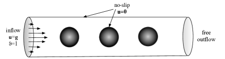
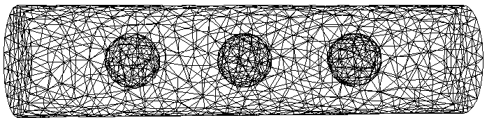
Figure 7: Left: illustration of the geometry and the boundary conditions. Right: coarsest mesh.

We conduct a mesh-refinement study on a series of three meshes with increasing resolution (cf. Fig. 7) in which we choose our time-steps according to the CFL stability condition. In Fig. 8, we compare our results at $t_{\rm end}=10$ for a non-conservative scheme as well as for the same series of experiments conducted with the conservatively coupled scheme. It can be observed that the flux-correction keeps the concentration profiles within physical bounds, and already a visual inspection reveals that it produces physically better solutions with less resolution than the uncorrected method. In the non-conservative case, we observe solution overshoots of around $100\%$ even for the finest mesh. The application of a simple limiter to these overshoots would take mass/energy out of the system, and thus we cannot expect reasonable results when using moderate resolutions with a straightforward coupling. The conservative mass-correction is a simple and elegant way to overcome this deficiency.

Figure 8: Cross-section in the $y/z$-plane of the computed solution on mesh-levels 0, 1, and 2 for the uncorrected scheme (left) and the corrected scheme (right); the plotting range is limited to $[0,1]$ in the left picture.

5.4.2 Non-isoviscous case

In the following, we consider two examples for the non-isoviscous case, both regarding simulations of the Earth mantle. Firstly, the full non-isothermal coupling of buoyancy-driven flow models, where we have a non-linear bidirectional coupling between flow and transport. In particular for this problem, the conservative coupling is crucial in order to avoid a spurious forcing on the velocity field as well as non-physical values of the temperature-dependent viscosity. Secondly, the simulation of the velocity field in the Earth mantle, where the boundary velocities for the Dirichlet condition on the surface and the temperature profile for the right-hand side are given by measured data. On the inner boundary, we use free-slip, i.e., $\mathbf{u}\cdot\mathbf{n}=(\nu D(\mathbf{u})\,\mathbf{n}-p\,\mathbf{n})\cdot\mathbf{t}_{i}=0$ where $\mathbf{t}_{i}$, $i=1,2$, denote the tangential vectors.

In these cases the momentum equation is given by

$$-\mathrm{div}(\nu D(\mathbf{u}))+\nabla p=\mathbf{f},$$ (38)

where $D(\mathbf{u})=1/2(\nabla\mathbf{u}+\nabla\mathbf{u}^{\top})$, denotes the symmetric part of the velocity gradient and $\mathbf{f}$ a temperature dependent forcing term. We consider in the following the spherical shell $\Omega=\{x\in\mathbb{R}^{3}:0.55<||x||_{2}<1\}$ as a computational domain with two different viscosities, either temperature depending or piecewise constant

$$\nu_{1}=e^{1/2-\vartheta},\qquad\nu_{2}=\begin{cases}1\quad&||x||_{2}<0.936,\\ 0.001&\text{else}.\end{cases}$$ (39)

For both examples the computational mesh is an icosahedral spherical mesh consisting of roughly a hundred million individual tetrahedra. For the first example with $\nu_{1}$, we consider thermal convection where the interior temperature at the boundary is set to $\vartheta(r=0.55)=1$ and at the surface to $\vartheta(r=1)=0$. Initially we prescribe an interpolation between core and surface temperature with a spherical harmonic perturbation. We solve the coupled problem with the previously described SCG multigrid solver for the Stokes part, coupled to an explicit time-integration of the finite-volume transport scheme with flux-correction for 11 500 time-steps on a mid-sized department cluster. A plot of a temperature iso-surface is depicted in Fig. 9 (left). For further details on the setup and the simulation parameters we refer to [33]. For the second example with the discontinuous viscosity $\nu_{2}$, where the jump roughly appears in the upper mantle (asthenosphere), we consider as a solver the Uzawa multigrid method, described in Sect. 4.1. A plot of the simulation result is depicted in Fig. 9 (right) which shows the typical behavior of the velocity field and the region of the viscosity jump.

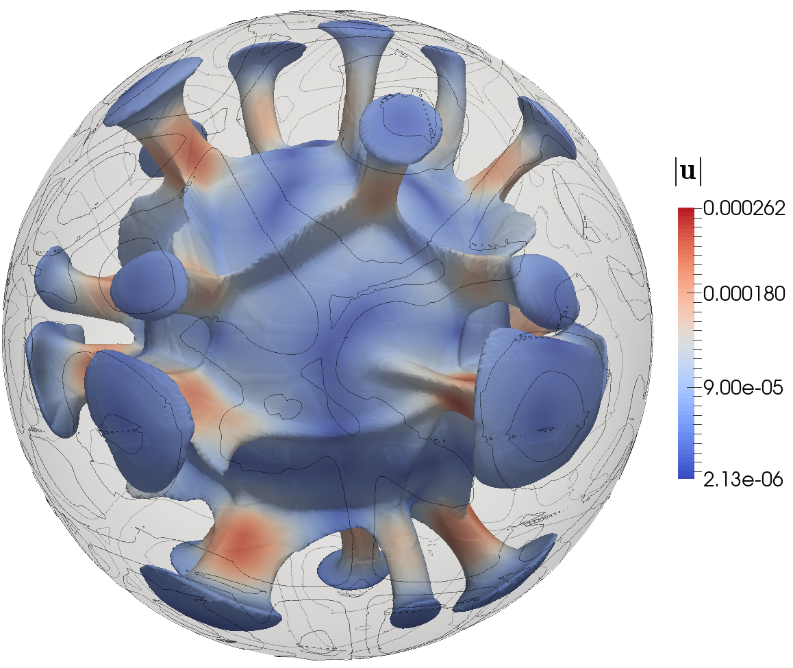
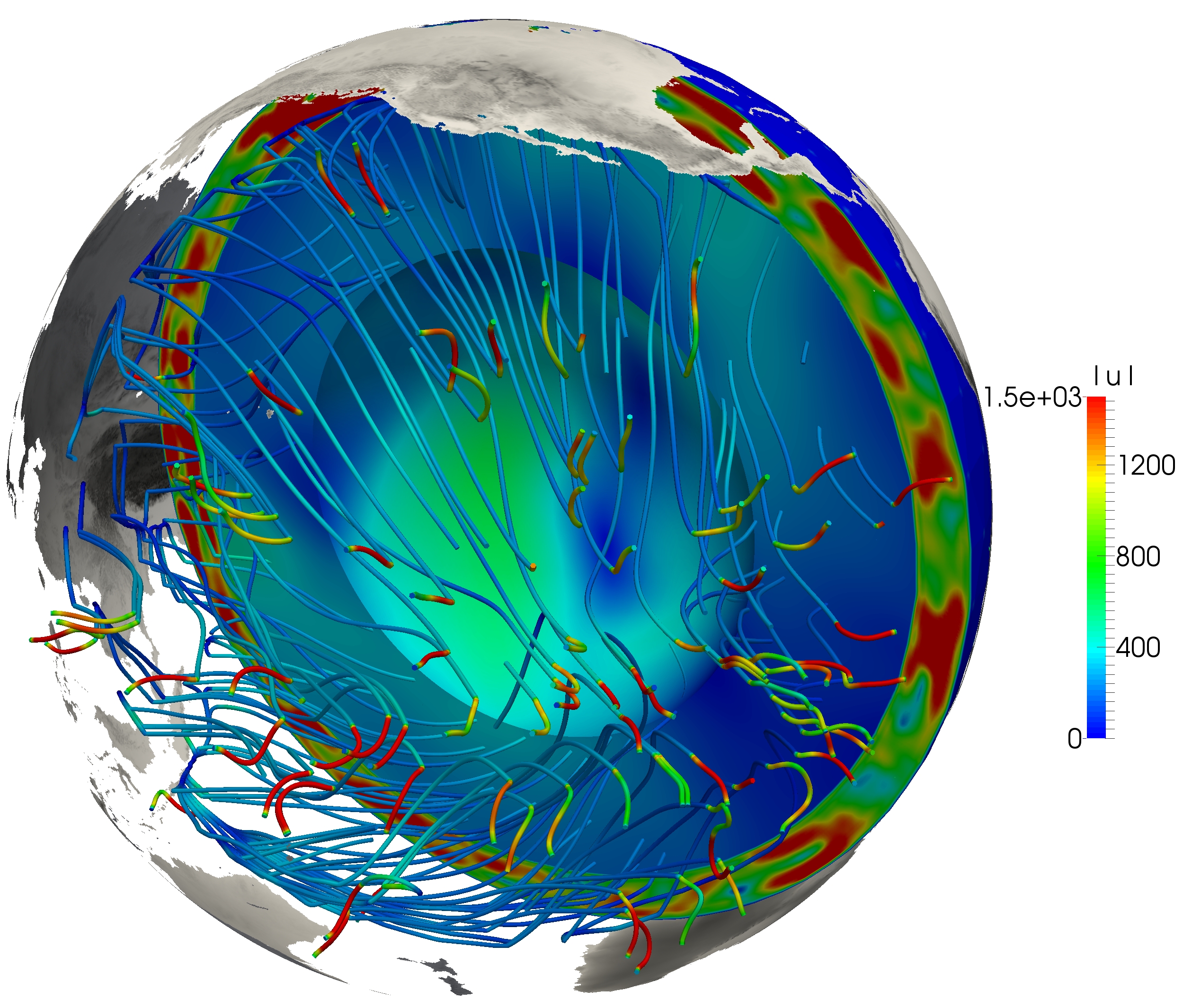
Figure 9: Iso-surfaces for $\vartheta=0.4$ colored by the velocity magnitude after 11 500 timesteps for $\nu_{1}$ (left) and magnitude of the velocity $\mathbf{u}$ for the real data simulation, including a viscosity jump $\nu_{2}$ (right).

Acknowledgements

The authors gratefully acknowledge the support by the Gauss Center for Supercomputing (GCS), the Jülich Supercomputing Centre (JSC), and the German Research Foundation (DFG) through the grants WO 671/14-1 and WO 671/11-1.

References

- [1] R. A. Adams and J. J. F. Fournier. Sobolev Spaces. Academic Press, New York, London, 2003.
- [2] D. N. Arnold, F. Brezzi, and M. Fortin. A stable finite element for the Stokes equations. Calcolo, 21(4):337–344, 1984.
- [3] R. E. Bank, B. D. Welfert, and H. Yserentant. A class of iterative methods for solving saddle point problems. Numer. Math., 56(7):645–666, 1990.
- [4] B. Bergen, T. Gradl, U. Rüde, and F. Hülsemann. A massively parallel multigrid method for finite elements. Computing in Science and Engineering, 8(6):56–62, 2006.
- [5] B. Bergen and F. Hülsemann. Hierarchical hybrid grids: data structures and core algorithms for multigrid. Numer. Linear Algebra Appl., 11:279–291, 2004.
- [6] H. Blum. The influence of reentrant corners in the numerical approximation of viscous flow problems. In Numerical treatment of the Navier-Stokes equations (Kiel, 1989), volume 30 of Notes Numer. Fluid Mech., pages 37–46. Vieweg, Braunschweig, 1990.
- [7] P. B. Bochev and C. R. Dohrmann. A stabilized finite element method for the Stokes problem based on polynomial pressure projections. Internat. J. Numer. Methods Fluids, 46(2):183–201, 2004.
- [8] D. Boffi, F. Brezzi, and M. Fortin. Mixed finite element methods and applications, volume 44 of Springer Series in Computational Mathematics. Springer, Heidelberg, 2013.
- [9] F. Brezzi, M. O. Bristeau, L. P. Franca, M. Mallet, and G. Rogé. A relationship between stabilized finite element methods and the Galerkin method with bubble functions. Comput. Methods Appl. Mech. Engrg., 96(1):117–129, 1992.
- [10] F. Brezzi and J. Douglas, Jr. Stabilized mixed methods for the Stokes problem. Numer. Math., 53(1-2):225–235, 1988.
- [11] M. Dauge. Stationary Stokes and Navier-Stokes systems on two- or three-dimensional domains with corners. I. Linearized equations. SIAM J. Math. Anal., 20(1):74–97, 1989.
- [12] H. Egger, U. Rüde, and B. Wohlmuth. Energy-corrected finite element methods for corner singularities. SIAM J. Numer. Anal., 52(1):171–193, 2014.
- [13] H. C. Elman, D. J. Silvester, and A. J. Wathen. Finite elements and fast iterative solvers: with applications in incompressible fluid dynamics. Oxford University Press, New York, 2005.
- [14] R. D. Falgout, J. E. Jones, and U. M. Yang. The design and implementation of hypre, a library of parallel high performance preconditioners. In Numerical solution of partial differential equations on parallel computers, volume 51 of Lect. Notes Comput. Sci. Eng., pages 267–294. Springer, Berlin, 2006.
- [15] S. Ganesan, G. Matthies, and L. Tobiska. Local projection stabilization of equal order interpolation applied to the Stokes problem. Math. Comp., 77(264):2039–2060, 2008.
- [16] F. J. Gaspar, Y. Notay, C. W. Oosterlee, and C. Rodrigo. A simple and efficient segregated smoother for the discrete Stokes equations. SIAM J. Sci. Comput., 36(3):A1187–A1206, 2014.
- [17] V. Girault and P. A. Raviart. Finite Element Methods for Navier-Stokes Equations. Springer, New York, 1986.
- [18] B. Gmeiner, U. Rüde, H. Stengel, C. Waluga, and B. Wohlmuth. Performance and Scalability of Hierarchical Hybrid Multigrid Solvers for Stokes Systems. SIAM J. Sci. Comput., 37(2):C143–C168, 2015.
- [19] B. Gmeiner, U. Rüde, H. Stengel, C. Waluga, and B. Wohlmuth. Towards textbook efficiency for parallel multigrid. Numer. Math. Theory Methods Appl., 8, 2015.
- [20] B. Gmeiner, C. Waluga, and B. Wohlmuth. Local mass-corrections for continuous pressure approximations of incompressible flow. SIAM J. Numer. Anal., 52(6):2931–2956, 2014.
- [21] B. Guo and C. Schwab. Analytic regularity of Stokes flow on polygonal domains in countably weighted Sobolev spaces. J. Comput. Appl. Math., 190(1-2):487–519, 2006.
- [22] M. Hagemann, O. Schenk, and A. Wächter. Matching–based preprocessing algorithms to the solution of saddle–point problems in large–scale nonconvex interior–point optimization. Comput. Optim. Appl., 36(2–3):321–341, 2007.
- [23] M. Huber, B. Gmeiner, U. Rüde, and B. Wohlmuth. Resilience for mutlgrid software at the extreme scale, 2015. Submitted.
- [24] L. John, P. Pustejovska, U. Rüde, and B. Wohlmuth. Energy-corrected finite element methods for the Stokes system, 2015. In preparation.
- [25] L. John, B. Wohlmuth, and W. Zulehner. On the Smoothing Properties of Block Preconditioners for Saddle Point Problems, 2015. In preperation.
- [26] V. A. Kondratiev. Boundary value problems for elliptic equations in domains with conical or angular points. Trans. Moscow Math. Soc., 16:227–313, 1967.
- [27] V. A. Kozlov, V. G. Mazya, and J. Rossmann. Spectral Problems Associated with Corner Singularities of Solutions to Elliptic Equations. Mathematical surveys and monographs. American Mathematical Society, 2001.
- [28] A. Kufner. Weighted Sobolev spaces. A Wiley-Interscience Publication. John Wiley & Sons, Inc., New York, 1985. Translated from the Czech.
- [29] P. Märkl and A.-M. Sändig. Singularities of the stokes system in polygons. Preprint-Reihe: Institut für Angewandte Analysis und Numerische Simulation, Universität Stuttgart, 2008/009, 2008.
- [30] U. Rüde, C. Waluga, and B. Wohlmuth. Nested Newton strategies for energy-corrected finite element methods. SIAM J. Sci. Comput., 36(4):A1359–A1383, 2014.
- [31] J. Schöberl and W. Zulehner. On Schwarz-type smoothers for saddle point problems. Numer. Math., 95(2):377–399, 2003.
- [32] R. Verfürth. A combined conjugate gradient-multigrid algorithm for the numerical solution of the Stokes problem. IMA J. Numer. Anal., 4(4):441–455, 1984.
- [33] C. Waluga, B. Wohlmuth, and U. Rüde. Mass-corrections for the conservative coupling of flow and transport on collocated meshes, 2015. Submitted.
- [34] W. Zulehner. Analysis of iterative methods for saddle point problems: a unified approach. Math. Comp., 71(238):479–505, 2002.