Maximum Hands-off Control without Normality Assumption

Abstract

Maximum hands-off control is a control that has the minimum $L^{0}$ norm among all feasible controls. It is known that the maximum hands-off (or $L^{0}$-optimal) control problem is equivalent to the $L^{1}$-optimal control under the assumption of normality. In this article, we analyze the maximum hands-off control for linear time-invariant systems without the normality assumption. For this purpose, we introduce the $L^{p}$-optimal control with $0<p<1$, which is a natural relaxation of the $L^{0}$ problem. By using this, we investigate the existence and the bang-off-bang property (i.e. the control takes values of $\pm 1$ and $0$) of the maximum hands-off control. We then describe a general relation between the maximum hands-off control and the $L^{1}$-optimal control. We also prove the continuity and convexity property of the value function, which plays an important role to prove the stability when the (finite-horizon) control is extended to model predictive control.

I INTRODUCTION

In some situations, the control effort can be dramatically reduced by hands-off control, holding the control value exactly zero over a time interval. The hands-off control is effective in hybrid/electric vehicles, railway vehicles, and networked/embedded systems [10, 11].

Motivated by these applications, recently, a novel control method, called maximum hands-off control, has been proposed in [9, 11]. The purpose of maximum hands-off control is to maximize the time duration where the control value is exactly zero among all feasible controls. The hands-off property is related to sparsity measured by the $L^{0}$ norm of a signal, defined by the total length of the intervals over which the signal takes non-zero values. This motivates the use of the cost function in which the control effort is penalized via the $L^{0}$ norm. The maximum hands-off control, in other words, seeks the sparsest (or $L^{0}$-optimal) control among all feasible controls, and hence the maximum hands-off control is also called sparse optimal control or $L^{0}$-optimal control.

A mathematical difficulty in the maximum hands-off control is the discontinuity and the non-convexity of the $L^{0}$ cost function. Hence, recent works [11, 6] have proposed to use the $L^{1}$ norm for enhancing sparsity, as often seen in compressed sensing [3, 4]. In [6], under the normality assumption (e.g. the plant model is controllable and the $A$-matrix is nonsingular), the equivalence is proved between the $L^{0}$-optimal control and the $L^{1}$-optimal control. The continuity and the convexity of the value function is also proved under the same assumption.

Alternatively, a very recent work [2] has proved the existence theorem of the maximum hands-off control without the normality assumption, by directly dealing with the maximum hands-off control problem without the aid of smooth or convex relaxation. As the necessary condition, any maximum hands-off control is also proved to have the bang-off-bang property. However, the sufficient condition for a control having the bang-off-bang property to be $L^{0}$-optimal is not obtained.

In the present article, we examine the maximum hands-off control without the normality assumption, by introducing the $L^{p}$-optimal control with $0<p<1$. As will be described in Section III, $L^{p}$-optimal control is a relaxation of the maximum hands-off (i.e. $L^{0}$-optimal) control. Indeed, the equivalence holds between the $L^{0}$-optimal control and the $L^{p}$-optimal control. The purpose of this article is not only to prove the existence and the bang-off-bang properties of the maximum hands-off control, but also to show a general relation between the maximum hands-off control and the $L^{1}$-optimal control. The relation leads to the sufficient and necessary condition for a control having the bang-off-bang property to be $L^{0}$-optimal, which is not obtained in the recent works. Also, it leads the equivalence between the value functions in the $L^{0}$-optimal and the $L^{1}$-optimal controls, by which we prove the convexity and the continuity of the value function. This property guarantees the stability when the (finite-horizon) maximum hands-off control is extended to model predictive control, as discussed in [7].

The remainder of this paper is organized as follows: In Section II, we give mathematical preliminaries for our subsequent discussion. In Section III, we define the maximum hands-off control problem, and investigate it via the $L^{p}$-optimal control. We show the existence and the bang-off-bang property of the maximum hands-off control and the relation between the maximum hands-off control and the $L^{1}$-optimal control. Section IV confirms the continuity and the convexity of the value function. Section V presents an example to illustrate the difference between the maximum hands-off control and the $L^{1}$-optimal control, by showing the existence of an $L^{1}$-optimal control that is not $L^{0}$-optimal. In Section VI, we offer concluding remarks.

II MATHEMATICAL PRELIMINARIES

This section reviews basic definitions, facts, and notation that will be used throughout the paper.

Let $n$ be a positive integer. For a vector $x\in{\mathbb{R}}^{n}$ and a scalar $\varepsilon>0$, the $\varepsilon$-neighborhood of $x$ is defined by

$${\mathcal{B}}(x,\varepsilon)\triangleq\{y\in\mathbb{R}^{n}:\|y-x\|<\varepsilon\},$$

where $\|\cdot\|$ denotes the Euclidean norm in ${\mathbb{R}}^{n}$. Let ${\mathcal{X}}$ be a subset of ${\mathbb{R}}^{n}$. A point $x\in{\mathcal{X}}$ is called an interior point of ${\mathcal{X}}$ if there exists $\varepsilon>0$ such that ${\mathcal{B}}(x,\varepsilon)\subset{\mathcal{X}}$. The interior of ${\mathcal{X}}$ is the set of all interior points of ${\mathcal{X}}$, and we denote the interior of ${\mathcal{X}}$ by $\mathrm{int}{\mathcal{X}}$. A point $x\in\mathbb{R}^{n}$ is called an adherent point of ${\mathcal{X}}$ if ${\mathcal{B}}(x,\varepsilon)\cap{\mathcal{X}}\neq\emptyset$ for every $\varepsilon>0$, and the closure of ${\mathcal{X}}$ is the set of all adherent points of ${\mathcal{X}}$. A set ${\mathcal{X}}\subset{\mathbb{R}}^{n}$ is said to be closed if ${\mathcal{X}}=\overline{{\mathcal{X}}}$, where $\overline{{\mathcal{X}}}$ is the closure of ${\mathcal{X}}$. The boundary of ${\mathcal{X}}$ is the set of all points in the closure of ${\mathcal{X}}$, not belonging to the interior of ${\mathcal{X}}$, and we denote the boundary of ${\mathcal{X}}$ by $\partial{\mathcal{X}}$, i.e., $\partial{\mathcal{X}}=\overline{{\mathcal{X}}}-\mathrm{int}{\mathcal{X}}$, where $\mathcal{X}_{1}-\mathcal{X}_{2}$ is the set of all points which belong to the set ${\mathcal{X}}_{1}$ but not to the set ${\mathcal{X}}_{2}$. A set ${\mathcal{X}}\subset{\mathbb{R}}^{n}$ is said to be convex if, for any $x,y\in{\mathcal{X}}$ and any $\lambda\in[0,1]$, $(1-\lambda)x+\lambda y$ belongs to ${\mathcal{X}}$.

A real-valued function $f$ defined on a convex set ${\mathcal{C}}\subset{\mathbb{R}^{n}}$ is said to be convex if

$$f\bigl{(}(1-\lambda)x+\lambda y\bigr{)}\leq(1-\lambda)f(x)+\lambda f(y),$$

for all $x$, $y\in\mathcal{C}$ and all $\lambda\in(0,1)$.

Let $T>0$. For a continuous-time signal $u(t)$ over a time interval $[0,T]$, we define its $L^{p}$ and $L^{\infty}$ norms respectively by

$$\|u\|_{p}\triangleq\bigg{\{}\int_{0}^{T}|u(t)|^{p}dt\bigg{\}}^{1/p},\quad\|u\|_{\infty}\triangleq\sup_{t\in[0,T]}|u(t)|,$$

where $p\in(0,\infty)$. Note that $\|\cdot\|_{p}$ for $p\in(0,\,1)$ is not a norm but a quasi-norm since it fails the triangle inequality [8]. We simply denote the set of all signals with $\|u\|_{p}<\infty$ by $L^{p}$ instead of $L^{p}[0,\,T]$. We define the $L^{0}$ norm of a signal $u$ on the interval $[0,T]$ as

$$\|u\|_{0}\triangleq m(\{t\in[0,T]:u(t)\neq 0\}),$$

where $m$ is the Lebesgue measure on ${\mathbb{R}}$. Note that $L^{0}$ “norm” is not a norm since it fails the homogeneity property, that is, for any non-zero scalar $\alpha$ such that $|\alpha|\neq 1$, we have $\|\alpha u\|_{0}=\|u\|_{0}\neq|\alpha|\|u\|_{0}$ for any $u\neq 0$. The notation $\|\cdot\|_{0}$ derives from the equation in Proposition 1.

III MAXIMUM HANDS-OFF CONTROL PROBLEM

In this paper, we consider a linear time-invariant system represented by

$$\dot{x}(t)=Ax(t)+Bu(t),\quad 0\leq t\leq T,$$ (1)

where $A\in\mathbb{R}^{n\times n}$, $B\in\mathbb{R}^{n\times 1}$, and $T>0$ is a fixed final time of control. We here assume single-input control for simplicity.

For the system (1), we call a control $u\in L^{1}$ feasible if it steers $x(t)$ from a given initial state $x(0)=\xi\in\mathbb{R}^{n}$ to the origin at time $T$ (i.e., $x(T)=0$) and satisfies the magnitude constraint $\|u\|_{\infty}\leq 1$. We denote by ${\mathcal{U}}(\xi)$ the set of all feasible controls for an initial state $\xi\in{\mathbb{R}}^{n}$, that is,

$$\mathcal{U}(\xi)\triangleq\biggl{\{}u\in L^{1}:\int_{0}^{T}e^{-At}Bu(t)dt=-\xi,\quad\|u\|_{\infty}\leq 1\biggr{\}}.$$

The control objective is to obtain a control $u\in{\mathcal{U}(\xi)}$ that has the maximum time duration on which $u(t)$ takes $0$. In other words, we seek the control that has the minimum $L^{0}$ norm among all feasible controls in ${\mathcal{U}}(\xi)$. This optimal control problem is called the maximum hands-off control problem. This is formulated as follows.

Problem 1 (maximum hands-off control problem)

For a given initial state $\xi\in\mathbb{R}^{n}$, find a feasible control $u\in\mathcal{U}(\xi)$ that minimizes

$$J(u)\triangleq\|u\|_{0}.$$

We call the optimal control the maximum hands-off control.

Note that the cost function $J(u)$ can be rewritten as

$$J(u)=\int_{0}^{T}\phi_{0}(u(t))~{}dt,$$

where $\phi_{0}$ is the $L^{0}$ kernel function defined by

$$\phi_{0}(u)\triangleq\begin{cases}1,&\text{~{}if~{}}u\neq 0,\\ 0,&\text{~{}if~{}}u=0.\end{cases}$$ (2)

Obviously, the kernel function $\phi_{0}(u)$ is discontinuous at $u=0$ and non-convex. Also, the cost function $J(u)$ is non-convex, and it has a strong discontinuity. Indeed, for any functions $u\neq 0$, $v=0$, and any scalar $\lambda\in(0,1)$, we have $\|\lambda u+(1-\lambda)v\|_{0}=\|u\|_{0}$. On the other hand, we have $\lambda\|u\|_{0}+(1-\lambda)\|v\|_{0}=\lambda\|u\|_{0}<\|u\|_{0}$. Although the sequence of constant functions $u_{k}=1/k$ on $[0,T]$ converges to $0$ uniformly, $J(u_{k})$ takes $T$ for any positive integer $k$, and hence it does not converge to $0$. In contrast, in this paper, we will show that the value function is continuous and convex on the domain.

First, we show the existence and the bang-off-bang property of maximum hands-off control via $L^{p}$-optimal control problem.

III-A $L^{p}$-Optimal Control

Here, we examine the $L^{p}$-optimal control problem, which is formulated as follows.

Problem 2 ($L^{p}$-optimal control problem)

For a given initial state $\xi\in\mathbb{R}^{n}$, find a feasible control $u\in\mathcal{U}(\xi)$ that minimizes

$$J_{p}(u)\triangleq\|u\|_{p}^{p},$$

where $p\in(0,\,1)$.

We call the solutions to this problem the $L^{p}$-optimal control, for which the following proposition is fundamental.

Proposition 1

For $f\in L^{1}$, we have

$$\|f\|_{0}=\lim_{p\to 0+}\|f\|_{p}^{p}.$$

Proof:

See Appendix. ∎

From now on, we show the existence and the bang-off-bang property of the $L^{p}$-optimal control. Let us define the set of all initial states for which there exist feasible controls, which is known as the reachable set at time $T$.

Definition 1

For the system (1), the reachable set $\mathcal{R}$ at time $T$ is defined by

$$\mathcal{R}\triangleq\bigg{\{}\int_{0}^{T}e^{-At}Bu(t)dt:\|u\|_{\infty}\leq 1\bigg{\}}\subset\mathbb{R}^{n}.$$

The following lemma states the existence and the bang-off-bang property.

Lemma 1

For each initial state in the reachable set $\mathcal{R}$, there exist $L^{p}$-optimal controls, and they take only $\pm 1$ and $0$ on the time interval $[0,\,T]$.

Proof:

The existence of $L^{p}$-optimal controls is shown in [12], and we here prove the bang-off-bang property.

Fix any initial state $\xi\in\mathcal{R}$, and take any $L^{p}$-optimal control $u^{\ast}(t)$ for the initial state $\xi$, and let $x^{\ast}$ denote the resultant state trajectory according to the control $u^{\ast}$.

The Hamiltonian function for the $L^{p}$-optimal control problem is defined as

$$H(x,\,q,\,u)\triangleq|u|^{p}+q^{\mathrm{T}}(Ax+Bu),$$ (3)

where $q\in\mathbb{R}^{n}$ is the costate vector. From Pontryagin’s minimum principle [1], there exists a costate vector $q^{\ast}$ that satisfies:

$$H(x^{\ast},\,q^{\ast},\,u^{\ast})\leq H(x^{\ast},\,q^{\ast},\,u),\quad\forall u\in\mathcal{U}(\xi),$$ (4)

$${\dot{x}^{\ast}(t)}=Ax^{\ast}(t)+Bu^{\ast}(t),\quad{\dot{q}^{\ast}(t)}=-A^{\mathrm{T}}q^{\ast}(t),$$

$$x^{\ast}(0)=\xi,\quad x^{\ast}(T)=0.$$

From (3) and (4), the $L^{p}$-optimal control $u^{\ast}$ is given by

$$u^{\ast}(t)=\mathop{\rm arg~{}min}\limits_{|u|\leq 1}\,|u|^{p}+(q^{\ast}(t))^{\mathrm{T}}Bu,\quad t\in[0,\,T].$$ (5)

Hence, from some elementary computation, we have

$$u^{\ast}(t)=\begin{cases}1,&\mbox{if }(q^{\ast}(t))^{\mathrm{T}}B<-1,\\ 0,&\mbox{if }-1<(q^{\ast}(t))^{\mathrm{T}}B<1,\\ -1,&\mbox{if }1<(q^{\ast}(t))^{\mathrm{T}}B,\\ 0\mbox{ or }1,&\mbox{if }(q^{\ast}(t))^{\mathrm{T}}B=-1,\\ -1\mbox{ or }0,&\mbox{if }(q^{\ast}(t))^{\mathrm{T}}B=1.\end{cases}$$ (6)

on $[0,T]$. This means that the $L^{p}$-optimal control $u^{\ast}(t)$ takes only $\pm 1$ and $0$ on $[0,\,T]$. ∎

From this lemma, we can show the equivalence between the maximum hands-off control and the $L^{p}$-optimal control.

Theorem 1

Let any initial state $\xi\in\mathcal{R}$ be fixed. Let $\mathcal{U}_{0}^{\ast}(\xi)$ and $\mathcal{U}_{p}^{\ast}(\xi)$ be the sets of all maximum hands-off (i.e. $L^{0}$-optimal) controls and all $L^{p}$-optimal controls, respectively. Then we have

$$\mathcal{U}_{0}^{\ast}(\xi)=\mathcal{U}_{p}^{\ast}(\xi).$$ (7)

Furthermore, we have

$$\|u_{0}\|_{0}=\|u_{p}\|_{p}^{p}$$ (8)

for any $u_{0}\in\mathcal{U}_{0}^{\ast}(\xi)$ and $u_{p}\in\mathcal{U}_{p}^{\ast}(\xi)$.

Proof:

From Lemma 1, we can take any $L^{p}$-optimal control $u_{p}(t)$, which takes only $\pm 1$ and $0$ on $[0,\,T]$. Then we have

$$\begin{aligned} \|u_{p}\|_{p}^{p}&=\int_{0}^{T}|u_{p}(t)|^{p}dt=\int_{\{t:u_{p}(t)\neq 0\}}|u_{p}(t)|dt\\ &=\int_{\{t:u_{p}(t)\neq 0\}}1dt=\|u_{p}\|_{0}.\end{aligned}$$ (9)

For any $u\in\mathcal{U}(\xi)$, we have

$$\begin{aligned} \|u\|_{p}^{p}&=\int_{0}^{T}|u(t)|^{p}dt=\int_{\{t:u(t)\neq 0\}}|u(t)|^{p}dt\\ &\leq\int_{\{t:u(t)\neq 0\}}1dt=\|u\|_{0}.\end{aligned}$$ (10)

From (9), (10) and the optimality of $u_{p}$, we have

$$\|u_{p}\|_{0}=\|u_{p}\|_{p}^{p}\leq\|u\|_{p}^{p}\leq\|u\|_{0}$$

for any $u\in\mathcal{U}(\xi)$. This gives $u_{p}\in\mathcal{U}_{0}^{\ast}(\xi)$, and hence $\mathcal{U}_{p}^{\ast}(\xi)\subset\mathcal{U}_{0}^{\ast}(\xi)$. Therefore the set $\mathcal{U}_{0}^{\ast}(\xi)$ is not empty.

Take any maximum hands-off control $u_{0}\in\mathcal{U}_{0}^{\ast}(\xi)$. From (10) and the optimality of $u_{0}$ and $u_{p}$, we have

$$\|u_{p}\|_{p}^{p}\leq\|u_{0}\|_{p}^{p}\leq\|u_{0}\|_{0}\leq\|u_{p}\|_{0}=\|u_{p}\|_{p}^{p},$$

which yields

$$\|u_{0}\|_{p}^{p}=\|u_{p}\|_{p}^{p},$$ (11)

$$\|u_{0}\|_{0}=\|u_{p}\|_{p}^{p}.$$ (12)

Equation (11) gives $\mathcal{U}_{0}^{\ast}(\xi)\subset\mathcal{U}_{p}^{\ast}(\xi)$, and hence (7) follows. Equation (12) means just the last statement (8). ∎

In summary, the maximum hands-off control is characterised as follows:

Theorem 2

For each initial state $\xi\in\mathcal{R}$, there exist maximum hands-off controls, and they take only $\pm 1$ and $0$ on $[0,\,T]$.

From the definition of the reachable set $\mathcal{R}$, this theorem states that the initial state $\xi$ exists in $\mathcal{R}$ if and only if maximum hands-off controls exist.

III-B Relation between Maximum Hands-Off Control and $L^{1}$-Optimal Control

We briefly review the $L^{1}$-optimal control problem based on the discussion in [1, Sec. 6-13], and confirm the definition of the normality.

In the $L^{1}$-optimal control problem, for a given initial state $\xi$, we seek the control that has the minimum $L^{1}$ norm among all feasible controls in ${\mathcal{U}}(\xi)$. The optimal controls are called $L^{1}$-optimal controls.

We apply the Pontryagin’s minimum principle. Assume that there exists an $L^{1}$-optimal control $u^{\ast}(t)$. Then there exists a vector $q^{\ast}(t)\in\mathbb{R}^{n}$ on $[0,T]$ such that

$$u^{\ast}(t)=\begin{cases}1,&\mbox{if }B^{\mathrm{T}}q^{\ast}(t)<-1,\\ 0,&\mbox{if }|B^{\mathrm{T}}q^{\ast}(t)|<1,\\ -1,&\mbox{if }B^{\mathrm{T}}q^{\ast}(t)>1.\end{cases}$$

$$u^{\ast}(t)\in[0,1],\quad\mspace{2.0mu}\mbox{if }B^{\mathrm{T}}q^{\ast}(t)=-1,$$

$$u^{\ast}(t)\in[-1,0],\,\,\mbox{if }B^{\mathrm{T}}q^{\ast}(t)=1.$$

Therefore, if $|B^{\mathrm{T}}q^{\ast}(t)|$ is not equal to $1$ at almost everywhere in $[0,T]$, then the $L^{1}$-optimal control $u^{\ast}(t)$ can be determined uniquely, and $u^{\ast}(t)$ takes only $0$ and $\pm 1$ on $[0,T]$. Then the $L^{1}$-optimal control problem is called normal.

Definition 2 (Normality)

Define the set

$$\mathcal{I}\triangleq\{t\in[0,\,T]:|B^{\mathrm{T}}q^{\ast}(t)|=1\}.$$

If $m(\mathcal{I})=0$, then the $L^{1}$-optimal control problem is said to be normal.

Theorem 2 reveals the general relation between maximum hands-off controls and $L^{1}$-optimal controls, which is a generalization of a result in [6].

Theorem 3

Fix any initial state $\xi\in\mathcal{R}$. Let $\mathcal{U}_{0}^{\ast}(\xi)$ and $\mathcal{U}_{1}^{\ast}(\xi)$ be the sets of all maximum hands-off controls and all $L^{1}$-optimal controls, respectively. Then we have

$$\mathcal{U}_{0}^{\ast}(\xi)\subset\mathcal{U}_{1}^{\ast}(\xi)$$ (13)

and

$$\|u_{0}\|_{0}=\|u_{1}\|_{1}$$ (14)

for any $u_{0}\in\mathcal{U}_{0}^{\ast}(\xi)$ and $u_{1}\in\mathcal{U}_{1}^{\ast}(\xi)$.

In particular, if the $L^{1}$-optimal control problem is normal, then we have $\mathcal{U}_{0}^{\ast}(\xi)=\mathcal{U}_{1}^{\ast}(\xi)$.

Proof:

From Theorem 2, we can take any maximum hands-off control $u_{0}(t)$, which takes only $\pm 1$ and $0$ on $[0,\,T]$. There exist a control $u_{1}\in\mathcal{U}_{1}^{\ast}(\xi)$ which takes only $\pm 1$ and $0$ on $[0,\,T]$, even if the $L^{1}$-optimal control problem fails the normality assumption [5]. Then we have

$$\|u_{0}\|_{0}=\|u_{0}\|_{1},\quad\|u_{1}\|_{1}=\|u_{1}\|_{0}.$$ (15)

From the optimality of $u_{0}$ and $u_{1}$, we also have

$$\|u_{0}\|_{0}\leq\|u_{1}\|_{0},\quad\|u_{1}\|_{1}\leq\|u_{0}\|_{1}.$$ (16)

It follows from (15) and (16) that

$$\|u_{0}\|_{1}=\|u_{1}\|_{1},\quad\|u_{0}\|_{0}=\|u_{1}\|_{1}.$$

The first equation yields the relation (13), and the second equation is (14). Finally, for the case under the normality assumption, see [6]. ∎

We note that any maximum hands-off control is always an $L^{1}$-optimal control, but the reverse does not necessarily hold. As seen in the proof, maximum hands-off controls are just $L^{1}$-optimal controls having the bang-off-bang property. More precisely, if the normality assumption fails, then there exists an $L^{1}$-optimal control which is not $L^{0}$-optimal. In Section V, we give such an example. In contrast, for every initial state, these optimal control problems always have the same optimal value.

IV VALUE FUNCTION

In this section, we investigate the value function in maximum hands-off control. The value function of an optimal control problem is defined as the mapping from initial states to the optimal values. The value functions in maximum hands-off control and $L^{1}$-optimal control are defined as

$$V(\xi)\triangleq\min_{u\in\mathcal{U}(\xi)}\|u\|_{0},\quad V_{1}(\xi)\triangleq\min_{u\in\mathcal{U}(\xi)}\|u\|_{1},$$

for $\xi\in\mathcal{R}$.

Here, we prove the continuity and the convexity of the value function $V(\xi)$ on $\mathcal{R}$ based on the discussion given in [7]. As proved there, these properties play an important role to prove the stability when the maximum hands-off control is extended to model predictive control.

First, let us show the convexity of $V(\xi)$.

Theorem 4

The value function $V(\xi)$ is convex on $\mathcal{R}$.

Proof:

It is sufficient to show the convexity of $V_{1}(\xi)$, since we have

$$V(\xi)=V_{1}(\xi),\quad\xi\in\mathcal{R}$$

from Theorem 3. Take any initial states $\xi$, $\eta\in\mathcal{R}$ and any scalar $\lambda\in(0,\,1)$. Let $u_{\xi}(t)$ and $u_{\eta}(t)$ be $L^{1}$-optimal controls for the initial state $\xi$ and $\eta$, respectively.

Obviously, the following control

$$u\triangleq(1-\lambda)u_{\xi}+\lambda u_{\eta}$$ (17)

steers the state from the initial state $(1-\lambda)\xi+\lambda\eta$ to the origin at time $T$, and it satisfies $\|u\|_{\infty}\leq 1$. That is, we have $u\in{\mathcal{U}}\bigl{(}(1-\lambda)\xi+\lambda\eta\bigr{)}$. Therefore we have

$$V_{1}(\lambda\xi+(1-\lambda)\eta) \leq\|\lambda u_{\xi}+(1-\lambda)\eta\|_{1}$$

$$\leq\lambda\|u_{\xi}\|_{1}+(1-\lambda)\|u_{\eta}\|_{1}$$

$$=\lambda V_{1}(\xi)+(1-\lambda)V_{1}(\eta),$$

which shows the convexity of the value function $V_{1}$. ∎

Next, we show the continuity of $V(\xi)$. For this, we prepare the following lemmas.

Lemma 2

For any scalar $\alpha\geq 0$, the following set

$$\mathcal{R}_{\alpha}\triangleq\{\xi\in\mathcal{R}:V(\xi)\leq\alpha\}$$

is closed.

Proof:

See the proof of [7, Lemma 4]. ∎

Lemma 3

The reachable set $\mathcal{R}$ is characterized by

$$\mathcal{R}=\{\xi\in\mathcal{R}:V(\xi)\leq T\}.$$ (18)

In particular, if the pair $(A,\,B)$ is controllable, then

$$\partial\mathcal{R}=\{\xi\in\mathcal{R}:V(\xi)=T\}.$$ (19)

Proof:

See the proof of [7, Lemma 5]. ∎

From these lemmas, we can show the continuity of the value function $V(\xi)$.

Theorem 5

If the pair $(A,\,B)$ is controllable, then $V(\xi)$ is continuous on $\mathcal{R}$.

Proof:

The proof is similar to the proof of [7, Theorem 6]. ∎

V EXAMPLE

Theorem 3 states that for a system that fails the normality assumption, there exists a control which is $L^{1}$-optimal but not $L^{0}$-optimal. Here, we give such an example.

Let us consider the double-integral system, which is modelled by

$${\dot{x}(t)}=\begin{pmatrix}0&1\\ 0&0\end{pmatrix}x(t)+\begin{pmatrix}0\\ 1\end{pmatrix}u(t),\quad 0\leq t\leq T.$$ (20)

Let the initial condition be

$$(x_{1}(0),\,x_{2}(0))=(\xi_{1},\,\xi_{2}),$$

where $x(t)=(x_{1}(t),\,x_{2}(t))^{\mathrm{T}}$ and $\xi_{i}\in\mathbb{R}$ for $i=1,\,2$.

From [1, Control Law 8-3], this system fails the normality assumption for the initial states satisfying

$$\frac{1}{2}\xi_{2}^{2}<\xi_{1},\quad\xi_{2}<0,\quad-\frac{\xi_{2}}{2}-\frac{\xi_{1}}{\xi_{2}}<T.$$ (21)

That is, the $L^{1}$-optimal control can not be determined uniquely for these initial states. The set of all $L^{1}$-optimal controls consists of all controls such that

$$0\leq u(t)\leq 1,\quad\forall t\in[0,T],$$

$$\int_{0}^{T}u(t)dt=-\xi_{2},\quad\int_{0}^{T}\int_{0}^{\theta}u(t)dtd\theta=-\xi_{1}-\xi_{2}T.$$

The dashed line in Fig. 1 shows such an $L^{1}$-optimal control $u_{1}(t)$ (obtained via numerical optimization) for the parameters

$$T=5,\quad\xi_{1}=1,\quad\xi_{2}=-1,$$ (22)

which satisfy the condition (21). Clearly, this $L^{1}$-optimal control $u_{1}(t)$ is not $L^{0}$-optimal.

On the other hand, the following is also one of the $L^{1}$-optimal controls for the initial state satisfying (21):

$$u_{2}(t)=\begin{cases}0,&\mbox{if }t\in[0,\,t_{1})\cup[t_{2},\,T],\\ 1,&\mbox{if }t\in[t_{1},\,t_{2}),\end{cases}$$

where

$$t_{1}=\frac{\xi_{2}}{2}-\frac{\xi_{1}}{\xi_{2}},\quad t_{2}=-\frac{\xi_{2}}{2}-\frac{\xi_{1}}{\xi_{2}}.$$

This gives a maximum hands-off control since the $L^{1}$-optimal control that takes only $\pm 1$ and $0$ is $L^{0}$-optimal as seen in the proof of Theorem 3. The solid line in Fig. 1 shows the control $u_{2}(t)$ for the parameters given in (22). Obviously, the control $u_{2}(t)$ has much smaller $L^{0}$ norm than that of $u_{1}(t)$. In other words, the control $u_{1}(t)$ is $L^{1}$-optimal, but it is not $L^{0}$-optimal.

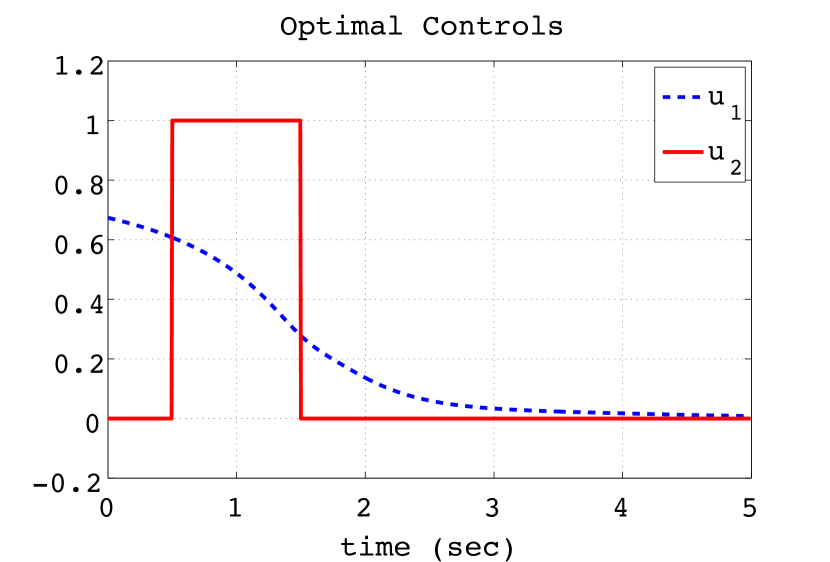
Figure 1: $L^{1}$-optimal control $u_{1}$ (dashed) and maximum hands-off control $u_{2}$ (solid)

VI CONCLUSION

In this paper, we have shown that among feasible controls there exists at least one maximum hands-off control, and it has the bang-off-bang property. This result is obtained by examining the $L^{p}$-optimal control for $0<p<1$, which is a natural relaxation for the $L^{0}$-optimal control. Indeed, we have shown the equivalence between the maximum hands-off control and the $L^{p}$-optimal control. This leads to the general relation between the maximum hands-off control and the $L^{1}$-optimal control, that is, any maximum hands-off control is given by an $L^{1}$-optimal control that has the bang-off-bang property, but an $L^{1}$-optimal control is not necessarily $L^{0}$-optimal in the absence of the normality assumption. As an example for this, we have given the double-integral system. Also we have proved the continuity and the convexity of the value function, which can be used to prove the stability in model predictive control.

APPENDIX

PROOF OF PROPOSITION 1

For $f\in L^{1}$, define

$$E\triangleq\{t\in[0,T]:|f(t)|\leq 1\},$$

$$F\triangleq\{t\in[0,T]:|f(t)|>1\}.$$

Then we have

$$\|f\|_{p}^{p}=\int_{E}|f(t)|^{p}dt+\int_{F}|f(t)|^{p}dt.$$

On the right hand side, if we take $p\to 0+$, the integrand of the first term increases, and that of the second term decreases. It follows from Lebesgue’s monotone convergence theorem [13] that

$$\lim_{p\to 0+}\|f\|_{p}^{p}=\int_{E}\phi_{0}(f(t))dt+\int_{F}\phi_{0}(f(t))dt=\|f\|_{0},$$

where $\phi_{0}$ is the $L^{0}$ kernel function defined by (2).