Theory of time reversal topological superconductivity in double Rashba wires – symmetries of Cooper pair and Andreev bound states

Abstract

We study the system of double Rashba wires brought into the proximity to an $s$-wave superconductor. The time reversal invariant topological superconductivity is realized if the interwire pairing corresponding to crossed Andreev reflection dominates over the standard intrawire pairing. We derive the topological criterion and show that the system hosts zero energy Andreev bound states such as a Kramers pair of Majorana fermions. We classify symmetry of the Cooper pairs focusing on the four degrees of freedom, $i.e.$, frequency, spin, spatial parity inside wires, and spatial parity between wires. The magnitude of the odd-frequency pairing is strongly enhanced in the topological state. We also explore properties of junctions occurring in such double wire systems. If one section of the junction is in the topological state and the other is in the trivial state, the energy dispersion of Andreev bound states is proportional to $\sim\pm\sin\varphi$, where $\varphi$ denotes the macroscopic phase difference between two sections. This behavior can be intuitively explained by the couplings of a Kramers pair of Majorana fermions and spin-singlet $s$-wave Cooper pair and can also be understood by analyzing an effective continuum model of the $s+p$/$s$-wave superconductor hybrid system.

I Introduction

The concept of topologySchnyder et al. (2008); Kitaev (2009) and topological effects has attracted a lot of attention over past decades. For example, the appearance of the zero energy surface Andreev bound state (SABS) in unconventional superconductors like $p$-wave Buchholtz and Zwicknagl (1981); Hara and Nagai (1986) or $d$-wave superconductors Hu (1994); Tanaka and Kashiwaya (1995); Kashiwaya and Tanaka (2000) has been understood in terms of the topological invariants defined for the bulk Hamiltonian. Sato et al. (2011); Tanaka et al. (2012); Kobayashi et al. (2014, 2015) Also the possibility to generate an effective topological $p$-wave superconductivity in the systems coupled to conventional $s$-wave superconductors due to internal spin structureSato and Fujimoto (2009); Lutchyn et al. (2010); Oreg et al. (2010); Alicea (2010); Chevallier et al. (2012); Klinovaja et al. (2012a); Alicea (2012); Klinovaja et al. (2012b); Beenakker (2013); Klinovaja et al. (2013); Nadj-Perge et al. (2013); Klinovaja and Loss (2014a); Ebisu et al. (2015) opened the field for experiments.Mourik et al. (2012); Deng et al. (2012a); Rokhinson et al. (2012); Das et al. (2012a); Nadj-Perge et al. (2014); Pawlak et al. (2015) In one dimensional systems, zero energy SABSs are Majorana fermions (MFs), which are of great importance for topological quantum computing. Nayak et al. (2008); Alicea et al. (2011)

In this context, it is useful to shed light on MF physics from different angles. One aspect not covered in literature on MFs is the symmetry of the Cooper pairs in the topological regime. Generally, if we consider such degree of freedom as time, space as well as spin, there are four possible symmetries of Cooper pairs: even-frequency spin-singlet even-parity (ESE), even-frequency spin-triplet odd-parity (ETO), odd-frequency spin-triplet even-parity (OTE) Berezinskii (1974) and odd-frequency spin-singlet odd-parity (OSO). Balatsky and Abrahams (1992); Coleman et al. (1997); Fuseya et al. (2003) It is known that odd-frequency pairing ubiquitously exists in inhomogeneous superconductors, Tanaka et al. (2007a, 2012) and it is hugely enhanced at the boundaries if zero energy SABSs are present. Tanaka and Golubov (2007); Tanaka et al. (2007a, b, 2012); Eschrig et al. (2007) The connection between MFs and odd-frequency pairing have also been clarified before in several systems. Asano and Tanaka (2013); Wakatsuki et al. (2014); Ebisu et al. (2015, 2015) It was shown that MFs inevitably accompany odd-frequency spin-triplet pairing in the D class topological superconductors with broken time-reversal symmetry.

Alternatively, there are also time reversal invariant topological superconductors belonging to the topological DIII classSchnyder et al. (2008); Kitaev (2009) and occuring in various condensed matter systems. Fu and Kane (2008); Fu and Berg (2010); Sasaki et al. (2011); Hsieh and Fu (2012); Yamakage et al. (2012); Klinovaja and Loss (2015a); Schrade et al. If the time reversal symmetry is not broken, two MFs come in Kramers pairs and protected from splitting.Fu and Kane (2009); Nakosai et al. (2012); Wong and Law (2012); Nakosai et al. (2013); Keselman et al. (2013); Gaidamauskas et al. (2014); Klinovaja et al. ; Zhang et al. (2013); Deng et al. (2012b); Klinovaja et al. (2014); Chung et al. (2013); Qi et al. (2009, 2010); Klinovaja and Loss (2014b) In this work we focus on the system consisting of two quantum wires with Rashba type spin-orbit interaction (SOI) brought into proximity to an $s$-wave superconductor as introduced in Ref. [Klinovaja and Loss, 2014b]. The interwire superconducting pairing induced by crossed Andreev processes is larger than the intrawire pairing due to strong electron-electron interactions. The crossed Andreev reflection, when two electrons forming initially the Cooper pair get separated into different channels, has attracted a special attention due to its potential use for creating entanglementRecher et al. (2001); Hannes and Titov (2008); Braunecker et al. (2013) and has been implemented in superconductor/normal metal/superconductor junctionsDeutscher and Feinberg (2000); Beckmann et al. (2004); Russo et al. (2005) and double quantum dots superconductor hybrid systems. Deutscher and Feinberg (2000); Recher et al. (2001); Recher and Loss (2002); Bena et al. (2002); Recher and Loss (2003); Beckmann et al. (2004); Russo et al. (2005); Hannes and Titov (2008); Hofstetter et al. (2009); Herrmann et al. (2010); Sato et al. (2010); Burset et al. (2011); Schindele et al. (2012); Das et al. (2012b); Sato et al. (2012); Braunecker et al. (2013)

Although the topological superconductivity and MFs have been already predicted for this model, the relation between Kramers MFs and odd-frequency pairing still remains largely unexplored for systems in the topological DIII class. For example, it is natural to expect that the spin structure of odd-frequency pairing in the presence of Kramers pairs is very different from one for the topological D class with a single MF. In addition, working with two quantum wires, we have to include one additional spatial degree of freedom such as the wire index.Parhizgar and Black-Schaffer (2014) We will call the superconducting pairing to be wire-odd (wire-even) if the pair amplitude picks up minus (plus) sign if one exchanges two wires. As a result, one can expect much richer structure of pairing amplitudes depending on four degrees of freedom, i.e., frequency, spin, and the spatial parity inside the wire as well as between the two wires. Besides symmetries of Cooper pairs, the energy of Andreev bound states (ABSs) in Josephson junctions has not been addressed in this system so far. All this together contributes to the advancement of the understanding of topological superconductor in DIII class and also of the physics of pairing symmetry.

The paper is organized as follows: In Sec. II, we introduce a tight-binding model of the double quantum wire (DQW) model with Rashba spin-orbit interaction and proximity induced superconductivity where both interwire and intrawire pairing potentials are taken into account. The topological criterion for the system is analyzed beyond the linearization approximation applied in Ref. [Klinovaja and Loss, 2014b]. We confirm that the interwire pairing potential must be larger than that of intrawire one and that the inversion symmetry should be broken. In Sec. III, we study symmetries of Cooper pair of the DQW model and find various types of pair amplitudes due to the translational and inversion symmetry breaking. We show that, in topological regime, the odd-frequency pairing is strongly enhanced at the ends of the system. We prove that the $\uparrow\downarrow$ component of the spin-triplet pairing is absent both for even and odd-frequency pairings due to the time reversal symmetry. In Sec. IV, we focus on ABSs in the DQW/normal metal/DQW and DQW/normal metal/spin-singlet $s$-wave superconductor Josephson junction system. Especially for the latter case, we see an anomalous energy dispersion of ABSs proportional to $\sim\pm\sin\varphi$ with $\varphi$ being the superconducting phase difference between two sections. We provide a qualitative argument to explain this relation by considering tunneling Hamiltonian between Kramers MFs and spin-singlet $s$-wave pairing. We also reproduce this dispersion relation in the framework of the effective model which can be interpreted as an $s+p$/$s$-wave superconducting junction. In Sec. V, we summarize our results.

II Model construction

We consider the setup consisting of two quantum wires with Rashba SOI proximity coupled to an $s$-wave superconductor (Fig. 1). The superconductivity in the DQW system could be induced in two different ways as described in Ref. [Klinovaja and Loss, 2014b]. The Cooper pair could tunnel as a whole into one of two wires resulting in the intrawire superconducting pairing. Alternatively, the Cooper pair could split such that electrons tunnel into different wires resulting into the interwire superconducting pairing also called the cross-Andreev superconducting pairing. We will work in the framework of tight-binding model with the Hamiltonian given by

$$H = -t\sum_{\left\langle i,j\right\rangle\sigma\eta}c_{i\sigma\eta}^{\dagger}c_{j\sigma\eta}-\sum_{i\sigma\eta}\mu_{\eta}c_{i\sigma\eta}^{\dagger}c_{i\sigma\eta}$$ (1)

$$+ i\sum_{\left\langle i,j\right\rangle\eta}\alpha_{\eta}\Bigl{(}c_{i\uparrow\eta}^{\dagger}c_{j\downarrow\eta}-c_{i\downarrow\eta}^{\dagger}c_{j\uparrow\eta}\Bigr{)}$$

$$+ \sum_{i\eta}\Delta_{\eta}\Bigl{(}c_{i\uparrow\eta}^{\dagger}c_{i\downarrow\eta}^{\dagger}+\text{H.c.}\Bigr{)}$$

$$+ \sum_{i}\Delta_{c}\Bigl{(}c_{i\uparrow 1}^{\dagger}c_{i\downarrow\bar{1}}^{\dagger}+c_{i\uparrow\bar{1}}^{\dagger}c_{i\downarrow 1}^{\dagger}+\text{H.c.}\Bigr{)}$$

Here, we introduce index $i$ ($\eta=1,\bar{1}$) to label lattice sites (QWs). We define $c_{i\sigma\eta}^{\dagger}(c_{i\sigma\eta})$ as the creation (annihilation) operator acting on the electron at the site $i$ of the $\eta$ QW with the spin $\sigma$ ($\sigma=\uparrow(\equiv 1),\downarrow(\equiv\bar{1})$). The first term represents hopping with amplitude $t$ between two adjacent sites $\left\langle i,j\right\rangle$. The second term describes chemical potential $\mu_{\eta}$ at each site. The third term corresponds to the Rashba SOI of the amplitude $\alpha_{\eta}$. The last two terms represent the intrawire and interwire pair potential with amplitude $\Delta_{\eta}$ and $\Delta_{c}$, respectively. To simplify analytical calculations, we focus on the case of $\Delta_{1}=\Delta_{\bar{1}}$ throughout this paper. Using translational invariance along $x$-direction, we introduce the number of unit cells $N_{x}$ and momentum in $x$-direction $k_{x}$, and Fourier transform the operators as $c_{i\sigma\eta}=\frac{1}{\sqrt{N_{x}}}\sum_{k_{x}}e^{ik_{x}a_{x}}c_{k_{x}\sigma\eta}$. The Hamiltonian can be rewritten in the momentum representation in the basis composed of $c_{k_{x}}=(c_{k_{x}\uparrow 1},c_{k_{x}\downarrow 1},c_{k_{x}\uparrow\bar{1}},c_{k_{x}\downarrow\bar{1}},c^{\dagger}_{-k_{x}\uparrow 1},c^{\dagger}_{-k_{x}\downarrow 1},c^{\dagger}_{-k_{x}\uparrow\bar{1}},c^{\dagger}_{-k_{x}\downarrow\bar{1}})^{T}$ as

$$\mathcal{H}(k_{x}) = \Big{[}\frac{\xi_{k_{x}1}}{2}\tau_{z}+\alpha_{1}\sin(k_{x}a_{x})\tau_{z}s_{y}\Big{]}(1+\eta_{z})$$ (2)

$$+ \Big{[}\frac{\xi_{k_{x}\bar{1}}}{2}\tau_{z}+\alpha_{\bar{1}}\sin(k_{x}a_{x})\tau_{z}s_{y}\Big{]}(1-\eta_{z})$$

$$- \Delta_{1}\tau_{y}s_{y}-\Delta_{c}\tau_{y}s_{y}\eta_{x}$$

Here, $s_{x,y,z},\tau_{x,y,z},$ and $\eta_{x,y,z}$ are Pauli matrices acting on the degree of freedom of spin, particle-hole, and chain, respectively. We define $\xi_{k_{x}\eta}$ as $\xi_{k_{x}\eta}=-2t\cos(k_{x}a_{x})-\mu_{\eta}$.

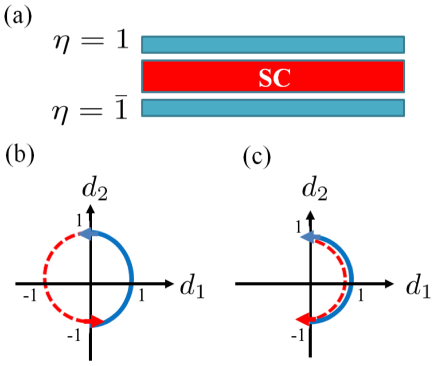
Figure 1: (a) A schematic picture of two Rashba QWs proximity coupled with superconductor. (b) The trajectory, spanned by the vector $(d_{1},d_{2})$ in the case $\text{sgn}[\lambda(k_{F,1})]=-\text{sgn}[\lambda(k_{F,2})]$, wraps around the origin leading to the topologically non-trivial state. (c) The trajectory, spanned by the vector $(d_{1},d_{2})$ in the case $\text{sgn}[\lambda(k_{F,1})]=\text{sgn}[\lambda(k_{F,2})]$, does not go around the origin which concludes that the system is topologically trivial.

By linearizing the energy spectrum, Klinovaja and Loss (2012)the authors in the work of Ref. [Klinovaja and Loss, 2014b] found that when $\Delta_{c}>\Delta_{1}$, time reversal invariant topological superconductor is realized. Here, we study this setup by tight-binding analysis to find whether time reversal invariant topological superconductor is obtained beyond the linearized approximation of the energy dispersion for arbitrary chemical potential.

Below, we calculate winding number to judge whether the system is topologically non-trivial. With an appropriate choice of the unitary transformation $V$, the Hamiltonian $H$ can be decomposed into two segments that are “time reversal partners” which are distinguished by index $l=1,2$. Then each sector is brought into off-diagonal form:

$$V^{\dagger}\mathcal{H}(k_{x})V=\left(\begin{array}[]{cc}\mathcal{H}_{1}(k_{x})&0\\ 0&\mathcal{H}_{2}(k_{x})\end{array}\right),$$ (3)

$$W^{\dagger}\mathcal{H}_{l}(k_{x})W=\left(\begin{array}[]{cc}0&h_{l}(k_{x})\\ h_{l}^{\dagger}(k_{x})&0\end{array}\right),$$ (4)

with the appropriate $8\times 8$ and $4\times 4$ matrices $V$ and $W$ (see Appendix A for more explicit forms). Below, we focus on $h_{1}(k_{x})$, however, we note that the topological condition remains the same if we consider $h_{2}(k_{x})$. The topological properties can be studied by evaluating the trajectory of determinant of $h_{1}(k_{x})$ X.G.Wen and A.Zee (1989) as a function of $k_{x}$ for $k_{x}a_{x}\in[-\pi,\pi)$,

$$\text{det}[h_{1}(k_{x})] =(\xi_{k_{x}1}-2\alpha_{1}\sin k_{x}a_{x}-i\Delta_{1})$$

$$\times(\xi_{k_{x}\bar{1}}-2\alpha_{\bar{1}}\sin k_{x}a_{x}-i\Delta_{1})+\Delta_{c}^{2}.$$ (5)

The system is topologically non-trivial when the trajectory of $\det[h_{1}(k_{x})]$ wraps around the origin in complex space, that is, the non-zero winding number indicates a non-trivial topological state. To simplify calculations, it is useful to introduce symmetric and antisymmetric parameters,

$$\alpha_{s/a} = (\alpha_{1}\pm\alpha_{\bar{1}})/2,$$

$$\mu_{s/a} = (\mu_{1}\pm\mu_{\bar{1}})/2.$$ (6)

The real and imaginary parts of det$[h_{1}(k_{x})]$ are rewritten as

$$\lambda(k_{x}) \equiv\text{Re}\bigl{[}\text{det}[h_{1}(k_{x})]\bigr{]}=-(\mu_{a}+2\alpha_{a}\sin k_{x}a_{x})^{2}+\Delta_{c}^{2}$$

$$\vspace{20 pt}-\Delta_{1}^{2}+(2t\cos k_{x}a_{x}+\mu_{s}+2\alpha_{s}\sin k_{x}a_{x})^{2},$$ (7)

$$\varepsilon(k_{x}) \equiv\text{Im}\bigl{[}\text{det}[h_{1}(k_{x})]\bigr{]}$$

$$\vspace{20 pt}=2\Delta_{1}(2t\cos k_{x}a_{x}+2\alpha_{s}\sin k_{x}a_{x}+\mu_{s}).$$ (8)

Here, we assume $\sqrt{4t^{2}+4\alpha_{s}^{2}}<|\mu_{s}|$ such that $\varepsilon(k_{x})$ becomes zero at certain values of $k_{x}$. Based on the spirit of “weak pairing limit”, Sato (2010); Qi et al. (2010) we discuss the winding number. X.G.Wen and A.Zee (1989) The winding number is equivalent to the number of wrapping of the normalized vector

$$(d_{1},d_{2})\equiv\left(\frac{\lambda(k_{x})}{\sqrt{\varepsilon^{2}(k_{x})+\lambda^{2}(k_{x})}},\frac{\varepsilon(k_{x})}{\sqrt{\varepsilon^{2}(k_{x})+\lambda^{2}(k_{x})}}\right)$$ (9)

around the origin in complex space as $k_{x}$ changes from $k_{x}a_{x}=-\pi$ to $k_{x}a_{x}=\pi$. We scale $\lambda(k_{x})$ to $\lambda(k_{x})\rightarrow a\lambda(k_{x})$ by introducing a parameter $a$, and continuously change $a$ from $a=1$ to a small non-zero value. Importantly, upon this change, the winding number remains the same. In the case of $\varepsilon(k_{x})\neq 0$, $(d_{1},d_{2})$ is approximated as $(0,{\rm sgn}\ \varepsilon(k_{x}))\equiv(0,\pm 1)$ for a sufficiently small $a$ and stays constant. However, in the vicinity of Fermi momenta $k_{F,j}$, which we define as two solutions of $\varepsilon(k_{F,j})=0$ such that $k_{F,1}<k_{F,2}$, the $(d_{1},d_{2})$ vector could wind around the origin. Close to these momenta, $\varepsilon(k_{x})$ can be expanded as

$$\varepsilon(k_{x})=[\partial_{k_{x}}\varepsilon](k_{x}-k_{F,j})+\cdots$$ (10)

At around the momentum $k_{F,j}$, the vector $(d_{1},d_{2})$ reads

$$d_{1} = \frac{a\lambda(k_{x})}{\sqrt{(\partial_{k_{x}}\varepsilon)^{2}(k_{x}-k_{F,j})^{2}+a^{2}\lambda^{2}(k_{x})}},$$

$$d_{2} = \frac{[\partial_{k_{x}}\varepsilon][(k_{x}-k_{F,j})]}{\sqrt{(\partial_{k_{x}}\varepsilon)^{2}(k_{x}-k_{F,j})^{2}+a^{2}\lambda^{2}(k_{x})}}.$$ (11)

Now we consider the trajectory spanned the the vector $(d_{1},d_{2})$ as the momentum changes from $k_{x}a_{x}=-\pi$ to $k_{x}a_{x}=\pi$, see also Fig. 1b. As we explained above, only parts of the trajectory close to $k_{x}=k_{F,1}$ and $k_{x}=k_{F,2}$ contribute to the winding number. Thus, we only focus on the trajectory around these momenta. If we consider $k_{x}$ changing as

$$(k_{x} < k_{F,1})\rightarrow(k_{x}=k_{F,1})\rightarrow(k_{F,1}<k_{x}<k_{F,2})$$

$$\rightarrow (k_{x}=k_{F,2})\rightarrow(k_{x}>k_{F,2}),$$

the vector $(d_{1},d_{2})$ changes accordingly as

$$(0,\text{sgn}[\varepsilon(k_{x}<k_{F,1})])\rightarrow(\text{sgn}[\lambda(k_{F,1})],0)\rightarrow(0,\text{sgn}[\varepsilon])$$

$$\rightarrow(\text{sgn}[\lambda(k_{F,2})],0)\rightarrow(0,\text{sgn}[\varepsilon(k_{x}>k_{F,2})]).$$

If $\text{sgn}[\lambda(k_{F,1})]=-\text{sgn}[\lambda(k_{F,2})]$, the trajectory of the vector $(d_{1},d_{2})$ wraps around the origin, see Fig. 1(b), indicating a topologically non-trivial state. On the other hand, if $\text{sgn}[\lambda(k_{F,1})]=\text{sgn}[\lambda(k_{F,2})]$, the trajectory does not wind around the origin, see Fig. 1(c), and the system is in the trivial state. Therefore, we can define the topological condition as follows,

$$(-1)^{\nu}=\prod_{\begin{subarray}{c}k_{x}=k_{F,1},k_{F,2}\end{subarray}}\text{sgn}[\Delta_{c}^{2}-\Delta_{1}^{2}-(\mu_{a}+2\alpha_{a}\sin k_{x}a_{x})^{2}],$$ (12)

where for $\nu=1(0)$ the system is non-trivial (trivial) topological state.

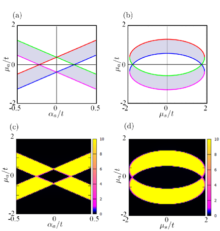
Figure 2: (a)[(b)]Topological phase diagram of DQW model as function of $\alpha_{a}$ and $\mu_{a}$ ($\mu_{s}$ and $\mu_{a}$) with $\Delta_{c}/t=0.4$, $\Delta_{1}/t=0.1$, and $\mu_{s}/t=-1$ ($\Delta_{c}/t=0.4$, $\Delta_{1}/t=0.1$, and $\alpha_{a}/t=0.5$ ). The light gray area represents topologically non-trivial phase. The red, green, blue, and magenta lines correspond to $\mu_{a}=2\alpha_{a}\mu_{0}+\sqrt{\Delta_{c}^{2}-\Delta_{1}^{2}},\mu_{a}=-2\alpha_{a}\mu_{0}+\sqrt{\Delta_{c}^{2}-\Delta_{1}^{2}},\mu_{a}=2\alpha_{a}\mu_{0}-\sqrt{\Delta_{c}^{2}-\Delta_{1}^{2}},$ and $\mu_{a}=-2\alpha_{a}\mu_{0}-\sqrt{\Delta_{c}^{2}-\Delta_{1}^{2}}$, respectively. (c)[(d)] The intensity plot of LDOS of zero energy on the edge of DQW model found by recursive Green’s function technique as function of as function of $\alpha_{a}$ and $\mu_{a}$ ($\mu_{s}$ and $\mu_{a}$) with $\Delta_{c}/t=0.4$, $\Delta_{1}/t=0.1$, and $\mu_{s}/t=-1$ ($\Delta_{c}/t=0.4$, $\Delta_{1}/t=0.1$, and $\alpha_{a}/t=0.5$ ). We set length of the system long enough (4000 sites) so that overlapping between zero energy states on the both edges is negligible. Rainis et al. (2013)Note that non-trivial area in (a)/(b) well corresponds to that of large amplitude of LDOS in (c)/(d).

First, we note from Eq. (12) that the condition $\Delta_{c}>\Delta_{1}$ has to be satisfied to realize topologically non-trivial state otherwise the product in Eq. (12) is always positive and the system is in the trivial state. Also, $\alpha_{a}$ should not be non-zero because only the term $\alpha_{a}\sin k_{x}a_{x}$ can produce the sign change of $[\Delta^{2}_{c}-\Delta_{1}^{2}-(\mu_{a}+2\alpha_{a}\sin k_{x}a_{x})^{2}]$ which leads minus sign of the product. Thus, the antisymmetric SOI is crucial for inducing the topologically non-trivial state. Otherwise, the SOI could be gauged away as was noted before in Ref. [Klinovaja and Loss, 2014b; Braunecker et al., 2010].

To get the explicit phase diagram for the system, we consider a simplified case by setting $\alpha_{s}=0$. In this case, the Fermi points $k_{F,1}$ and $k_{F,2}$ are defined via

$$\varepsilon(k_{x})=-2t\cos k_{x}a_{x}-\mu_{s}=0,$$ (13)

and are given by

$$k_{F,1}a_{x}=-\arcsin[\mu_{0}],\ k_{F,2}a_{x}=\arcsin[\mu_{0}].$$ (14)

with $\mu_{0}\equiv\sqrt{1-(\mu_{s}/2t)^{2}}$ for $|\mu_{s}|<2t$. According to Eq. (12),

$$(-1)^{\nu}={\rm sgn}\Bigl{[}\Delta_{c}^{2}-\Delta_{1}^{2}-(\mu_{a}+2\alpha_{a}\mu_{0})^{2}]$$

$$\times{\rm sgn}\Bigl{[}\Delta_{c}^{2}-\Delta_{1}^{2}-(\mu_{a}-2\alpha_{a}\mu_{0})^{2}\Bigr{]}.$$ (15)

has to result in $\nu=-1$ to realize the topological phase. For $\alpha_{a}\mu_{a}>0$, Eq. (15) is equivalent to

$$|\mu_{a}+2\alpha_{a}\mu_{0}|>\sqrt{\Delta_{c}^{2}-\Delta_{1}^{2}}>|\mu_{a}-2\alpha_{a}\mu_{0}|$$ (16)

have to be satisfied in order to get non-trivial state. In Fig. 2(a) [2(b)], we show the phase diagram of the DQW system as a function of $\alpha_{a}$ and $\mu_{a}$ ($\mu_{s}$ and $\mu_{a}$) with fixed $\Delta_{c}$, $\Delta_{1}$, and $\mu_{s}$ ($\Delta_{c}$, $\Delta_{1}$, and $\alpha_{a}$). The obtained results are in a good agreement with the results obtained in the tight-binding framework, as the non-zero LDOS at zero energy on edge of the DQW system indicate, see Fig. 2(c) and 2(d).

To summarize this section, two conditions, $\Delta_{c}>\Delta_{1}$ and $\alpha_{a}\neq 0$, are necessarily but not sufficient to generate time reversal invariant topological superconductivity. As we show in the next section, the presence of zero energy state also changes the dominant symmetries of Cooper pairs at the end of the system.

III Cooper pair symmetry

In this section, we study symmetries of Cooper pair in the model of double Rashba QW system coupled to an $s$-wave superconductor. In addition to the standard symmetries of Cooper pair, where frequency, spin, and parity are taken into account, we should include one more spatial degree of freedom connecting to two QWs. We call the pair amplitude to be wire-odd (wire-even) if it picks up negative sign (remains the same) by the exchange of the wire index. Due to this additional degree of freedom, there are now eight classes of Cooper pair with different symmetries that are consistent with Fermi-Dirac statistics as summarized in Table 1. These classes are i) even-frequency spin-singlet even-parity even-wire (ESEE), ii) even-frequency spin-singlet odd-parity odd-wire (ESOO), iii) even-frequency spin-triplet odd-parity even-wire (ETOE), iv) even-frequency spin-triplet even-parity odd-wire (ETEO), v) odd-frequency spin-singlet odd-parity even-wire (OSOE), vi) odd-frequency spin-singlet even-parity odd-wire (OSEO), vii) odd-frequency spin-triplet even-parity even-wire (OTEE), and viii) odd-frequency spin-triplet odd-parity odd-wire (OTOO).

	Frequency	Spin	Parity	Wire	Total
ESEE	+(Even)	-(Singlet)	+(Even)	+(Even)	-(Odd)
ESOO	+(Even)	-(Singlet)	-(Odd)	-(Odd)	-(Odd)
ETOE	+(Even)	+(Triplet)	-(Odd)	+(Even)	-(Odd)
ETEO	+(Even)	+(Triplet)	+(Even)	-(Odd)	-(Odd)
OSOE	-(Odd)	-(Singlet)	-(Odd)	+(Even)	-(Odd)
OSEO	-(Odd)	-(Singlet)	+(Even)	-(Odd)	-(Odd)
OTEE	-(Odd)	+(Triplet)	+(Even)	+(Even)	-(Odd)
OTOO	-(Odd)	+(Triplet)	-(Odd)	-(Odd)	-(Odd)

Table 1: All possible symmetries of Cooper pairs occurring in the double QW system.

The odd-frequency pairings combined with even-wire symmetry cases, v) and vii), have been studied in previous work dedicated to ferromagnet junctions, unconventional superconductor junctions, and non-uniform superconducting sytems. Bergeret et al. (2001, 2005); Eschrig et al. (2003); Asano et al. (2007a); Fominov et al. (2007); Braude and Nazarov (2007); Asano et al. (2007b); Yokoyama et al. (2007); Eschrig and Löfwander (2008); Eschrig (2015); Keizer et al. (2006); Sosnin et al. (2006); Khaire et al. (2010); Robinson et al. (2010); Sprungmann et al. (2010); Anwar et al. (2010); Tanaka and Golubov (2007); Tanaka et al. (2007a, b); Eschrig et al. (2007); Tanaka et al. (2012) The odd-frequency pairings combined with odd-wire symmetry, vi) and viii), have been discussed in bulk multi band (orbital) systems Black-Schaffer and Balatsky (2013); Komendová et al. (2015); Asano and Sasaki (2015) and two-channel Kondo lattice model. Hoshino (2014) In the present model, we consider both two effects.

First, we discuss how to evaluate pairing amplitudes. Using Eq. (1), we define Matsubara Green’s function as follows:

$$G_{M}(\omega_{n},j,j^{\prime},\sigma,\sigma^{\prime},\eta,\eta^{\prime})=\Bigl{(}\frac{1}{i\omega_{n}-H}\Bigr{)}_{j,j^{\prime},\sigma,\sigma^{\prime},\eta,\eta^{\prime}}$$ (17)

with Matsubara frequency which is set to be $\omega_{n}/t=0.01$ throughout the paper without loss of generality. Introducing matrices $G(\omega_{n},j,j^{\prime},\sigma,\sigma^{\prime},\eta,\eta^{\prime})$ and $F(\omega_{n},j,j^{\prime},\sigma,\sigma^{\prime},\eta,\eta^{\prime})$, we rewrite Eq. (17) as

$$G_{M}=\left(\begin{array}[]{cc}G&F\\ \tilde{F}&\tilde{G}\end{array}\right),$$ (18)

where $G_{M}$ is divided into four sectors in the particle-hole space. We focus on $F(\omega_{n},j,j^{\prime},\sigma,\sigma^{\prime},\eta,\eta^{\prime})$ to analyze symmetries of Cooper pairs. First, we focus on the frequency dependence. Introducing $J\equiv(j,j^{\prime},\sigma,\sigma^{\prime},\eta,\eta^{\prime}$), we define $F_{\text{O}}(J)$ and $F_{\text{E}}(J)$ as follows

$$F_{\mathfrak{A}}(J)=\frac{F(\omega_{n};J)+\text{sgn}[\mathfrak{A}]F(-\omega_{n};J)}{2}.$$ (19)

Here, we define $\mathfrak{A}=$E, O with the convention that sgn$[\text{E}/\text{O}]=\pm 1$. Then, using Eq. (19) and defining $K$ as $K\equiv(\sigma,\sigma^{\prime},\eta,\eta^{\prime})$, we introduce $F_{\text{OO}}(j;K),F_{\text{OE}}(j;K),F_{\text{EO}}(j;K),$ and $F_{\text{EE}}(j;K)$ classified also by the spatial symmetry inside the QW as

$$F_{\mathfrak{A}\mathfrak{B}}(j;K) = \frac{1}{2}\Bigl{\{}F_{\mathfrak{A}}(j+\frac{1-\text{sgn}[\mathfrak{B}]}{2},j)$$

$$+ \text{sgn}[\mathfrak{B}]F_{\mathfrak{A}}(j,j+\frac{1-\text{sgn}[\mathfrak{B}]}{2})\Bigr{\}},$$

with $\mathfrak{B}=$E, O. Further, by denoting $L$ as $L\equiv(\sigma,\sigma^{\prime})$, we can address the spacial symmetry between QWs defined by $F_{\mathfrak{A}\mathfrak{B}\text{O}}(j;L)$, $F_{\mathfrak{A}\mathfrak{B}\text{E}}(j;L)$ as

$$F_{{\mathfrak{A}\mathfrak{B}\mathfrak{C}}}(j;L)=\frac{F_{\mathfrak{A}\mathfrak{B}}(j;L;1,\bar{1})+\text{sgn}[\mathfrak{C}]F_{\mathfrak{A}\mathfrak{B}}(j;L;\bar{1},1)}{2},$$ (21)

with $\mathfrak{C}=$E, O. Finally, by addressing also the spin degree of freedom, we get eight classes of pair amplitude which are given by

$$F^{\uparrow\downarrow}_{\mathfrak{A}\text{T}\mathfrak{B}\mathfrak{C}}(j)=\frac{F_{\mathfrak{A}\mathfrak{B}\mathfrak{C}}(j;\uparrow,\downarrow)+F_{\mathfrak{A}\mathfrak{B}\mathfrak{C}}(j;\downarrow,\uparrow)}{2}$$ (22)

$$F_{\mathfrak{A}\text{S}\mathfrak{B}\mathfrak{C}}(j)=\frac{F_{\mathfrak{A}\mathfrak{B}\mathfrak{C}}(j;\uparrow,\downarrow)-F_{\mathfrak{A}\mathfrak{B}\mathfrak{C}}(j;\downarrow,\uparrow)}{2},$$ (23)

where the indices $\mathfrak{A},\mathfrak{B},$ and $\mathfrak{C}$ take the values either E or O. The combination of $\mathfrak{A},\mathfrak{B},$ and $\mathfrak{C}$ has to satisfy

$$\text{sgn}[\mathfrak{A}]\text{sgn}[\mathfrak{B}]\text{sgn}[\mathfrak{C}]=-1(+1)$$ (24)

for spin-triplet (spin-singlet) pairing. As for $\uparrow\uparrow$ and $\downarrow\downarrow$ spin-triplet components, the corresponding pair amplitudes are

$$F^{\uparrow\uparrow}_{\mathfrak{A}\text{T}\mathfrak{B}\mathfrak{C}}(j)=F_{\mathfrak{A}\text{T}\mathfrak{B}\mathfrak{C}}(j,\uparrow,\uparrow)$$ (25)

$$F^{\downarrow\downarrow}_{\mathfrak{A}\text{T}\mathfrak{B}\mathfrak{C}}(j)=F_{\mathfrak{A}\text{T}\mathfrak{B}\mathfrak{C}}(j,\downarrow,\downarrow).$$ (26)

We emphasize that due to the time reversal symmetry present in the system, the $\uparrow\downarrow$ components of spin-triplet are absent. Indeed, using the definition of anomalous Green function

$$F^{{\dagger}}(\omega_{n},j,j^{\prime},\sigma,\sigma^{\prime},\eta,\eta^{\prime})$$ (27)

$$\hskip 40.0pt\equiv\int_{0}^{\beta}d\tau e^{i\omega_{n}\tau}\left\langle c^{{\dagger}}(\tau)_{j,\sigma,\eta}c^{{\dagger}}(0)_{j^{\prime},\sigma^{\prime},\eta^{\prime}}\right\rangle,$$

$$F(\omega_{n},j,j^{\prime},\sigma,\sigma^{\prime},\eta,\eta^{\prime})$$ (28)

$$\hskip 40.0pt\equiv\int_{0}^{\beta}d\tau e^{i\omega_{n}\tau}\left\langle c(\tau)_{j,\sigma,\eta}c(0)_{j^{\prime},\sigma^{\prime},\eta^{\prime}}\right\rangle$$

with imaginary time $\tau$ and inverse temperature $\beta=1/k_{B}T$, as well as the fact that

$$c(\tau)_{j,\uparrow,\eta}\overset{\mathfrak{T}}{\rightarrow}-c(\tau)_{j,\downarrow,\eta}$$ (29)

$$c(\tau)_{j,\downarrow,\eta}\overset{\mathfrak{T}}{\rightarrow}c(\tau)_{j,\uparrow,\eta}$$ (30)

under time reversal operation $\mathfrak{T}$, we obtain

$$\mathfrak{T}[F(M;\uparrow,\downarrow;N)+F(M;\downarrow,\uparrow;N)]\mathfrak{T}^{-1}$$

$$=-[F(M^{\prime}\downarrow,\uparrow;N)+F(M^{\prime}\uparrow,\downarrow;N)]$$ (31)

for the time-reversal invariant system. Using the fact that Green’s function in Eq. (18) is invariant under time reversal operation we conclude that the $\uparrow\downarrow$ components of spin-triplet are absent. Above we used notations $M\equiv(\omega_{n},j,j^{\prime})$, $M^{\prime}\equiv(-\omega_{n},j,j^{\prime})$, and $N\equiv(\eta,\eta^{\prime})$. By similar argument, we show that $\uparrow\uparrow$ and $\downarrow\downarrow$ components are equal.

The Eqs. (22)-(26) describe all possible types of pair amplitudes that are also represented in Table 1. Before we begin with numerical calculations, we clarify general properties of the Hamiltonian and resulting symmetries of pairing amplitudes. First, we consider the infinite DQWs model. We start from the case with $\mu_{a}=0$, $\alpha_{s}=0$ and $\alpha_{a}=0$. In this case, only the ESEE pairing is present. This is the standard pairing for $\Delta_{1}$ and $\Delta_{c}$ originating from an $s$-wave superconductor without any symmetry breaking in double wire and spin-rotational spaces as well as without breaking of the translational invarience. As shown in Table 2, by breaking these symmetries, seven additional types of superconducting pairing are induced. In case (1), we break only the double wire symmetry by adding non-zero $\mu_{a}$. Now, the double-wire-even and double-wire-odd pairings can mix without changing symmetries in the spin space and without breaking the translational invarience. To be consistent with Fermi-Dirac statistics, the parity in the frequency space should be switched, thus the OSEO pairing is induced. In case (2), only $\alpha_{s}$ is chosen to be nonzero, thus, the spin rotational symmetry and spatial parity inside wire are broken at the same time. Then, the ETOE pairing is induced without generating odd-frequency pairing as was shown before in non-centrosymmetric superconductors with Rashba SOI. Yada et al. (2009) Next, in the case (3), the induced symmetries can be understood by combining the results of the cases (1) and (2). In addition to the ESEE pairing, the OTOO, OSEO, ETOE pairings are induced by the coexistence of $\mu_{a}$ and $\alpha_{s}$. We note that the presence of asymmetric Rashba coupling $\alpha_{a}$ also corresponds to the case (3), as it breaks the double wire symmetry and plays a role similar to $\alpha_{s}$ in the spin space.

Next, we consider systems, in which the translation invariance is also broken, for example, if some parameters are non-uniform or the system is finite. Thus, the parity mixing can occur by reversing the parity corresponding to frequency Tanaka et al. (2007a, b, 2012) to be consistent with Fermi-Dirac statistics. We first consider the case of $\mu_{s}=0$ and $\alpha_{s}=0$. In case (4), the breakdown of the parity inside a wire induces the OSOE pairing. This result is consistent with preexisting results in non-uniform superconducting systems. Tanaka et al. (2007a, b); Yokoyama et al. (2008); Tanaka et al. (2012) The obtained induced pairings in case (5) can be understood by combining the results of cases (1) and (4). The ESOO pairing is induced by the breakdown of the translational invarience and the double wire symmetry. Also the results in the case (6) can be understood by combining the results in the cases (2) and (4). The OTEE pairing is induced from the ETOE pairing by breaking of the translation invariance. The most interesting situation is the case (7). The OSEO, ETOE and OTOO pairings stem from results in the case (3). Similar to the case (4), the OSOE, ESOO, OTEE and ETEO pairings are generated by the spatial parity mixing due to the fact that the translation invariance is broken.

		Broken symmetry		Pairing symmetry
	DQW	spin	translation
	$\mu_{a}$	$\alpha_{s}$	boundary
(0)	–	–	–	ESEE
(1)	$\bigcirc$	–	–	ESEE, OSEO
(2)	–	$\bigcirc$	–	ESEE, ETOE
(3)	$\bigcirc$	$\bigcirc$	–	ESEE, OSEO, ETOE, OTOO
(4)	–	–	$\bigcirc$	ESEE, OSOE
(5)	$\bigcirc$	–	$\bigcirc$	ESEE, OSEO, OSOE, ESOO
(6)	–	$\bigcirc$	$\bigcirc$	ESEE, ETOE, OSOE, OTEE
(7)	$\bigcirc$	$\bigcirc$	$\bigcirc$	ESEE, OSEO, ETOE, OTOO
				OSOE, ESOO, OTEE, ETEO

Table 2: Eight classes of the possible symmetries of Cooper pairs in the DQW system. The classes are characterized by broken symmetries. The symmetry between two QWs composing the DQW system could be broken by detuning of the chemical potential. The spin space symmetry could be broken by the SOI. The translational invarience is broken, for example, by boundary conditions. The label $\bigcirc$ (– ) indicates that the symmetry is broken (preserved).

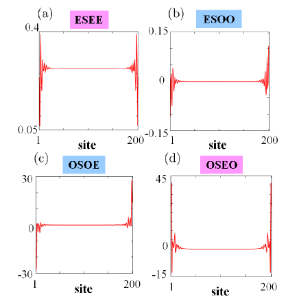
Figure 3: The spatial profiles of four singlet pairing amplitudes (denoted above each figure) for the DQW system of the finite size of 200 sites. The parameters are set to be as follows: $\alpha_{1}/t=-\alpha_{\bar{1}}/t=0.5,\mu_{1}/t=-2,\mu_{\bar{1}}/t=-1,\Delta_{1}/t=0.1,$ and $\Delta_{c}/t=0.4$. We confirm that the odd-frequency pairing amplitudes are strongly enhanced at both edges as panels (c) and (d) show.

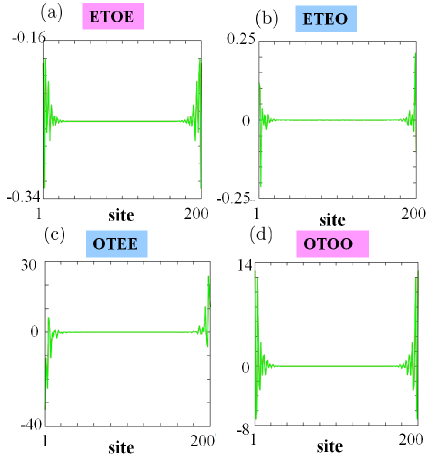
Figure 4: The spatial profiles of four triplet pairing amplitudes. The parameters are the same as in Fig. 3. Again, the odd-frequency pairing amplitudes peak at the edges, where Kramer pairs of MFs are located, see panels (c) and (d)

We calculate the spatial profile of pairing amplitudes numerically for parameters chosen such that the system is in the topological regime, see Figs. 3 and 4. First, odd-frequency components, $i.e.$ the magnitudes of the pairing amplitudes of OSEO, OTOO, OSOE, and OTEE, are hugely enhanced at the system edge in consistence with the existence of zero energy state, i.e., Kramers Majorana fermions, similar to the previous results obtained in unconventional superconductors. Tanaka and Golubov (2007); Tanaka et al. (2007a, b) Second, in addition to the ESEE pairing, which is the primary symmetry of the parent system [see Fig. 3(a)], the ETOE pairing spreads over the system [see Fig. 4(a)]. Although the OTOO and OSEO pairings are possible in the bulk from the discussion of the pairing symmetries (see above in Table 2), their magnitudes are small. The ESOO and ETEO pairing strengths are small and non-zero only at the system edge due to the breakdown of translational symmetry. To understand the spatial profile of these pairing amplitudes, it is convenient to focus on the inversion parity of the pairing amplitudes around the center of the quantum wire. As seen from Figs. 3 and 4, the inversion parity is even for the ESEE, OSEO, ETOE, OTOO pairings. These pairings can exist also in the bulk. In contrast to that, the inversion parities of the OSOE, ESOO, OTEE, ETEO pairings are odd. They are generated due to the breakdown of the translational invariance and localized at the edges.

To emphasize the correspondence between zero energy states and odd-frequency pairings explicitly, we calculated numerically the LDOS at the edge of the DQW system and the pairing amplitudes of OSEO and OTEE (see Fig. 5) for three different cases. The pairing amplitudes [see Figs. 5(b)-(e)] change as a function of energy similar to the LDOS [see Fig. 5(a)]. Specifically, when parameters are set to satisfy the topological criterion (blue line in Fig. 5), the real parts of the OSEO and OTEE pairing amplitudes change abruptly around zero energy. Importantly, the imaginary parts of the OSEO and OTEE pairing amplitudes peak strongly at zero energy, confirming the connection between the presence of the MFs and the odd-frequency pairing.

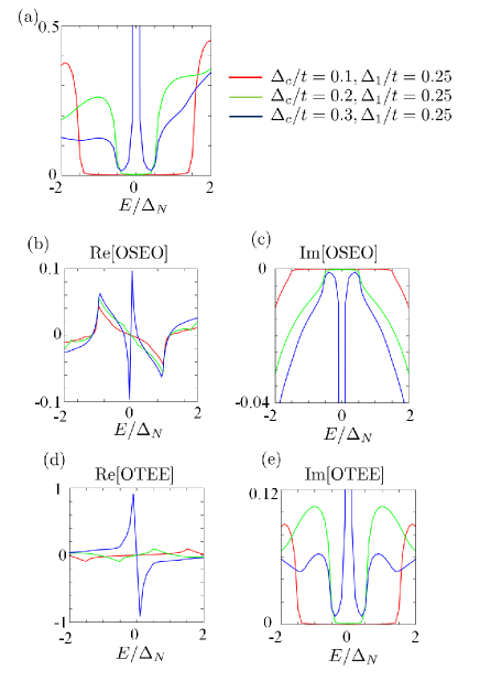
Figure 5: (a) The LDOS on the edge of the DQW system of the length of 4000 sites. (b-c) The real and imaginary parts of the OSEO pairing. (d-e): The real and imaginary parts of the OTEE pairing. Plots are based on recursive the Green function technique. The parameters are set as follows, $\alpha_{1}/t=-\alpha_{\bar{1}}/t=0.5$, $\mu_{1}/t=-2$, and $\mu_{\bar{1}}/t=-1$.

IV Josephson junction of DQWs

In this section, we address Andreev bound states (ABSs) in DQW/DQW junctions. The ABSs localized between two superconductors are extensively studied in the literature. The energy of the ABS $E_{b}$ localized between two topologically trivial $s$-wave superconductors is given by $E_{b}=\pm\sqrt{1-\sigma_{N}\sin^{2}(\varphi/2)}\Delta_{0}$, where $\Delta_{0}$, $\varphi$, and $\sigma_{N}$ is the magnitude of the superconducting pairing potential, the phase difference between superconductors and the transparency of the junctions, respectively. Furusaki and Tsukada (1991a) On the other hand, the energy of ABS $E_{b}$ between two one-dimensional topological $p_{x}$-wave superconductors is given by $E_{b}=\pm\sqrt{\sigma_{N}}\Delta_{0}\cos\varphi/2$.Kwon et al. (2004a); Kitaev (2001) The similar result is also known from the study of $d$-wave superconductor junctions. Tanaka and Kashiwaya (1997); Kashiwaya and Tanaka (2000) The present anomalous $\varphi$ dependence of the ABS can be explained by the coupling of MFs on both sides in Kitaev chain/Kitaev chain Josephson junction system.Kitaev (2001) It also generates $4\pi$ periodicity of the AC Josephson current in the Josephson junctions based on topological superconductors. In this section, we calculate the energy of the ABSs and find anomalous $\sim\pm\sin\varphi$ dependence. We provide qualitative explanation of this sinusoidal curve by considering the coupling of the Kramers pair of MFs to an $s$-wave superconductor. We also construct the effective model, which address the $s+p$/$s$-wave superconductor junctions, to explain this phase dependence of the ABS energy.

Making use of the recursive Green’s function technique, we can calculate the spectrum and the energy of the ABSs. First, we focus on the case when both sides of the DQWs are in the non-trivial topological regime. The result is shown in Fig. 6(a). This behavior is similar to the case of Kitaev chain/Kitaev chain or $p$-wave/$p$-wave junction system which demonstratesKitaev (2001) $\sim\pm\cos\varphi/2$. By introducing $\gamma_{\uparrow}$ and $\gamma_{\downarrow}$ to describe two different MFs building up the Kramers pair, we can understand the curve in Fig. 6(a) by the coupling of $\gamma_{\uparrow}$ and $\gamma_{\downarrow}$ on both sides, analogously to the mentioned above Kitaev chain/Kitaev chain junction. If the signs of the Rashba SOI is reversed on the right side, the spectrum of the ABSs is trivially shifted by $\pi$, as shown in Fig. 6(b). This is an example of the so-called $0$-$\pi$ transition: by reversing the sign of the Rashba term, the phase of effective $p$-wave superconductor is flipped by $\pi$. This transition has been already discussed in the system of a Rashba quantum wire on a superconductor with applied Zeeman fields, where topological superconductivity of the class D is realized.Ojanen (2013); Spånslätt et al. (2015); Klinovaja and Loss (2015b) Indeed, the observed behavior [see Fig. 6(b)] can also be explained by the above mentioned transition using the effective model of DQWs discussed below.

Next, we check the most interesting regime in which we set the one side of the junction to be in the topological regime and another to be in the trivial regime [see, Fig. 6(c)]. The energy spectrum of the ABSs follows $\sim\pm\sin\varphi$. This feature can be explained by the coupling of Kramers pair of MFs and to the $s$-wave superconductor as we demonstrate below.

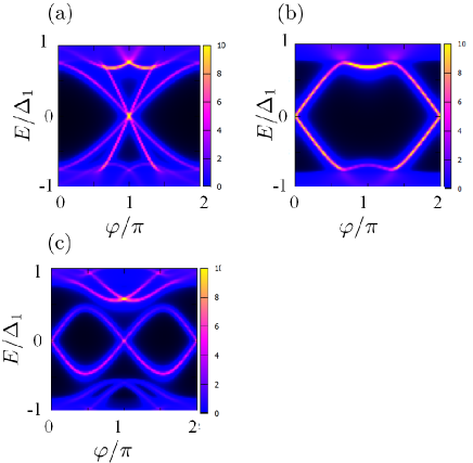
Figure 6: (a) The spectrum of the ABSs in the DQWs/normal metal/DQWs junction as a function of the phase difference $\varphi$. The parameters are set to be the same on both sides and correspond to the topologically non-trivial regime: $\alpha_{1}/t=-\alpha_{\bar{1}}/t=0.5,\mu_{1}/t=-2,\mu_{\bar{1}}/t=-1,\Delta_{1}/t=0.1,$ and $\Delta_{c}/t=0.4$. The ABSs behave like $\sim\pm\cos{\varphi/2}$. (b) Next, we reverse the signs of the Rashba SOI on the right side, $i.e.$, $\alpha_{1}/t=-\alpha_{\bar{1}}/t=-0.5$, other parameters are set to be the same as in the panel (a). The ABSs exhibit the $\pi$-shift and their energy behaves like $\sim\pm\sin{\varphi/2}$. (c) The right side of the system is brought into the trivial regime with parameters chosen to be $\alpha_{1}/t=\alpha_{\bar{1}}/t=0,\mu_{1}/t=-1,\mu_{\bar{1}}/t=-1,$ and $\Delta_{1}/t=0.1$. The ABSs near Fermi energy level behave like $\sim\pm\sin{\varphi}$. For all figures the calculation is based on recursive Green’s function technique, and we set the length of the right and left superconducting sections (normal metal section) to 4000 (2) lattice sites. The chemical potential in the normal section is set to $\mu_{N}/t=-1$.

The tunneling Hamiltonian can be written as

$$H_{T}=\sum_{k\sigma}\Bigl{(}T_{k}\gamma_{\sigma}b_{k\sigma}+\text{h.c.}\Bigr{)},$$ (32)

where $T_{k}$ is the tunneling amplitude, $b_{k\sigma}$ is the annihilation operator acting on the electron on the ride side of the junction with the spin $\sigma$ and the momentum $k$. The Majorana operator $\gamma_{\sigma}$ acts on the left side of the junction with the index $\sigma$ used to distinguish between to two MFs building a Kramers pair. We introduce the Bogoliubov transformation as follows

$$b_{k\uparrow} = u_{k}\alpha_{k\uparrow}+v^{*}_{k}\alpha_{-k\downarrow}^{\dagger}$$

$$b_{k\downarrow} = u_{-k}\alpha_{k\downarrow}-v^{*}_{-k}\alpha_{-k\uparrow}^{\dagger},$$ (33)

where $u_{k}$ and $v_{k}$ are given by

$$u_{k}=\frac{1}{2}\sqrt{1+\frac{\xi_{k}}{E_{k}}},\ \ v_{k}=\frac{1}{2}\sqrt{1-\frac{\xi_{k}}{E_{k}}}\exp(i\varphi),$$

and $\varphi$ is the macroscopic phase difference between right and left superconductors. Here, $\xi_{k}$ is the energy spectrum of the right superconductor in the normal state and $E_{k}=\sqrt{\xi_{k}^{2}+|\Delta_{k}|^{2}}$ is the quasi-particle energy spectrum, where $\Delta_{k}$ is the pair potential in the right side superconductor. Without loss of generality, $u_{k}$ can be set to be a real number and $v_{k}$ to be a complex number. As a result, the tunneling Hamiltonian is rewritten as

$$H_{T}=\sum_{k}\Bigl{\{}T_{k}\gamma_{\uparrow}(u_{k}\alpha_{k\uparrow}+v^{*}_{k}\alpha_{-k\downarrow}^{\dagger})+T_{k}^{\ast}(u_{k}\alpha_{k\uparrow}^{\dagger}+v_{k}\alpha_{-k\downarrow})\gamma_{\uparrow}$$

$$+T_{k}\gamma_{\downarrow}(u_{-k}\alpha_{k\downarrow}-v^{*}_{-k}\alpha_{-k\uparrow}^{\dagger})+T_{k}^{\ast}(u_{-k}\alpha_{k\downarrow}^{\dagger}-v_{-k}\alpha_{-k\uparrow})\gamma_{\downarrow}\Bigr{\}}.$$ (34)

At the next step, we construct the effective Hamiltonian describing the coupling between two MFs in the second order perturbation theory,

$$H_{\text{MF}}=\left\langle 0\right|H_{T}\frac{1}{E-H_{0}}H_{T}\left|0\right\rangle,$$ (35)

where $H_{0}$ represents BdG Hamiltonian without tunneling (32), $H_{0}\equiv\sum_{k\sigma}E_{k}\alpha_{k\sigma}^{\dagger}\alpha_{k\sigma}$, and $\left|0\right\rangle$ is set to be the ground-state of the quasi-particles. From Eq. (35), one finds

$$H_{T}\left|0\right\rangle=\sum_{k}(T_{k}v_{k}\gamma_{\uparrow}\alpha_{-k\downarrow}^{\dagger}-T_{k}^{\ast}u_{k}\gamma_{\uparrow}\alpha_{k\uparrow}^{\dagger}-T_{k}v_{-k}\gamma_{\downarrow}\alpha_{-k\uparrow}^{\dagger}-T_{k}^{\ast}u_{-k}\gamma_{\downarrow}\alpha_{k\downarrow}^{\dagger})\left|0\right\rangle,$$ (36)

$$\left\langle 0\right|H_{T}=\left\langle 0\right|\sum_{k^{\prime}}(T_{k^{\prime}}^{\ast}v_{k^{\prime}}^{\ast}\alpha_{-k^{\prime}\downarrow}\gamma_{\uparrow}-T_{k^{\prime}}u_{k^{\prime}}\alpha_{k^{\prime}\uparrow}\gamma_{\uparrow}-T_{k^{\prime}}^{\ast}v_{-k^{\prime}\uparrow}^{\ast}\alpha_{-k^{\prime}}\gamma_{\downarrow}-T_{k^{\prime}}u_{-k^{\prime}}\alpha_{k^{\prime}\downarrow}^{\dagger}\gamma_{\downarrow}),$$ (37)

$$H_{\text{MF}}=-\sum_{k}\frac{|T_{k}|^{2}}{E_{k}}\Bigl{\{}2u_{k}^{2}+2|v_{k}|^{2}+\bigl{(}\frac{\Delta_{k}}{2E_{k}}-\frac{\Delta_{k}^{\ast}}{2E_{k}}\bigr{)}\gamma_{\uparrow}\gamma_{\downarrow}-\bigl{(}\frac{\Delta_{k}}{2E_{k}}-\frac{\Delta_{k}^{\ast}}{2E_{k}}\bigr{)}\gamma_{\downarrow}\gamma_{\uparrow}\Bigr{\}}.$$ (38)

Here, we used the fact that $u_{k}=u_{-k}$, $v_{k}=v^{*}_{-k}$, and $T_{k}=T^{*}_{-k}$. and also set $E=0$. First, we ignore the first two terms in Eq. (38) because they are constant by noting $u_{k}^{2}+|v_{k}|^{2}=1$. If we impose the phase difference between the left and right superconductors as $\Delta_{k}\rightarrow\bar{\Delta}_{0}e^{i\varphi}$, $H_{\text{MF}}$ can be written in the basis of $(\gamma_{\uparrow},\gamma_{\downarrow})^{T}$ as

$$H_{\text{MF}}=\sum_{k}\bar{\Delta}_{0}\frac{|T_{k}|^{2}}{E_{k}^{2}}\sin\varphi\left(\begin{array}[]{cc}0&-i\\ i&0\end{array}\right).$$ (39)

with the energies given by $\pm\frac{|T_{k}|^{2}}{E_{k}^{2}}\bar{\Delta}_{0}\sin\varphi$, which coincides with the dispersion relation obtained for the ABSs in Fig.  6(c).

The characteristic features of the energy dispersion of the ABSs shown in Fig. 6(c) are also reproduced by the quasi-classical theory based on the effective model discussed in Ref. [Gaidamauskas et al., 2014]. Following Ref. [Gaidamauskas et al., 2014], we treat the terms breaking the symmetry between QWs as perturbations. Converting the lattice model back to continuous one, the effective Hamiltonian is written as

$$\mathcal{H}_{qk}=(\frac{\hbar^{2}k_{x}^{2}}{2m}-2t-\mu_{s})\tau_{z}-(\Delta_{s}+k_{x}s_{y}\Delta_{p})s_{y}\tau_{y},$$ (40)

$$\Delta_{s}=\Delta_{1}-\Delta_{c}+\frac{\mu_{a}^{2}+k_{x}^{2}\alpha_{a}^{2}}{\Delta_{1}+\Delta_{c}},$$ (41)

$$\Delta_{p}=2\frac{\alpha_{a}\mu_{a}}{\Delta_{1}+\Delta_{c}},$$ (42)

where $m$ is the effective mass given by $m=\hbar^{2}/2ta_{x}^{2}$. As seen from Eq. (42), if the signs of Rashba SOI are reversed, the phase of effective $p$-wave pair potential is shifted by $\pi$, which explains the 0-$\pi$ transition in Fig. 6(b). For simplicity, we set the $s$-wave pair potential to be determined at the Fermi momentum

$$\Delta_{s} = \Delta_{1}-\Delta_{c}+\frac{\mu_{a}^{2}+k_{F}^{2}\alpha_{a}^{2}}{\Delta_{1}+\Delta_{c}}$$ (43)

$$= \Delta_{1}-\Delta_{c}+\frac{\mu_{a}^{2}+2m(2t+\mu_{s})\alpha_{a}^{2}}{\Delta_{1}+\Delta_{c}}.$$

If we set $\Delta_{p}>\Delta_{s}/\sqrt{2m(2t+\mu_{s})}$, time reversal topological superconductivity is realized.Gaidamauskas et al. (2014) The effective Hamiltonian describes a one-dimensional $s$+$p$-wave superconductor. Generally, it is known that if $p$-wave component of the pair potential is larger than $s$-wave component, topological superconductor hosting edge states is realized.Tanaka et al. (2009a)

Next, we show that the behavior of ABSs obtained in Fig. 6(c) can be explained using the effective model of a semi-infinite $s$/$s$+$p$-wave junction. We consider the pair potential on $s$+$p$-wave side to be given by Eqs. (41) and (42), while on the $s$-wave side, it has the form $\Delta_{s}s_{y}\tau_{y}$ with $\Delta_{s}=\Delta_{0}e^{i\varphi}$. We assume that $\mu$ and $t$ are the same on both sections of the junction. However, two sets of values are chosen such that one corresponds to the topological phase and another to the trivial phase. We also take into account the strength of the interface barrier denoted by $Z$ but its value does not influence on the key feature of our results. In order to calculate ABSs, we seek the solution of $M\hat{y}=0$ where $\hat{y}$ is the envelope function composed of all the coefficients of the out-going modes (see Appendix B). Then, the ABSs can be obtained from the condition $\det M=0$. To make our plots more clear, we show $\left|\det M\right|^{\frac{1}{4}}$ as a function of energy $E$ and phase difference $\varphi$. The deep blue curve indicated the ABSs in Figs. 7(a) and 7(c). In the topological phase, where the $p$-wave pairing is dominant, we can see that the energy of ABSs is described by $\pm\sin\varphi$ around Fermi energy level, which is similar to the behaviour observed above in the lattice model [see Fig. 6 (c)]. Thus, the Josephson current-phase relation is approximated also by non-trivial dependence $\sim\sin 2\varphi$ as shown in 7(b), apart from standard $2\pi$-periodicity. Importantly, the observed double crossing points of ABSs around Fermi energy, in spite of the fact that the non-zero interface barrier $Z$ is explicitly introduced in the continuum model, confirm the topological origin of the obtained ABSs (MFs). As for the topologically trivial case in Fig. 7(c), where $s$-wave component is dominant, the ABSs behave as $\sim\sqrt{1-\sigma_{N}\sin^{2}\varphi}$. The corresponding current-phase relation has the standard $\sim\sin\varphi$ feature [see Figs. 7(d)]. It is also seen that the ABSs are gaped around zero energy due to the presence of the interface barrier, which reveals its trivial non-topological nature.

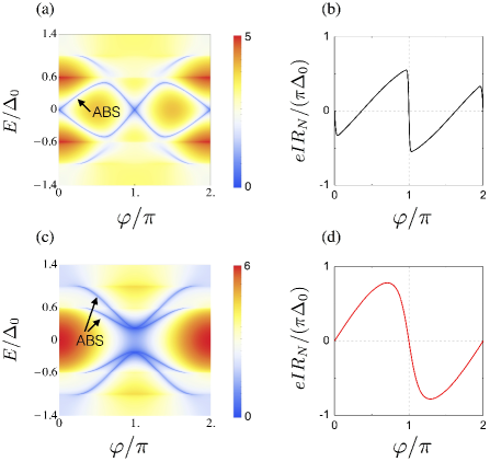
Figure 7: Illustration of ABSs and Josephson currents of $s$+$p$-wave/$s$-wave junction produced by continuum model. Panels (a) and (c) show $\left|\det M\right|^{\frac{1}{4}}$ where the deep blue curve shows the position of ABSs. Panels (b) and (d) show the current-phase relation normalized to the interface resistance $R_{N}$ in the normal state. (a) and (b): $\Delta_{0}/\tilde{\mu}=0.001$, $\Delta_{s}/\tilde{\mu}=0.0004$, $k_{F}\Delta_{p}/\tilde{\mu}=0.001$ and $\tilde{\mu}=2t+\mu_{s}$. (c) and (d): $\Delta_{0}/\tilde{\mu}=0.001$, $\Delta_{s}/\tilde{\mu}=0.001$, and $k_{F}\Delta_{p}/\tilde{\mu}=0.0004$. We use $Z=0.5$ for all cases and set the temperature $k_{B}T=0.01\Delta_{0}$ for the panels (b) and (d). Notice that when $p$-wave is dominant, the ABSs near Fermi energy has $\sim\sin\varphi$ feature which corresponds to non-trivial/trivial junction case as shown in Fig. 6(c).

V Conclusion

In this paper, we have studied the double quantum wire system brought into proximity to an $s$-wave superconductor. As was shown before, the system is in the topological phase if the induced interwire (crossed Andreev) pairing dominates. We have generalized this topological criterion to account for the detuning of the chemical potential by calculating the winding number. We have also classified symmetry of the superconducting order parameter by focusing on four degrees of freedom, $i.e.$, frequency, spin, the spatial parity inside the QWs, and the spatial parity between the QWs. The magnitude of the odd-frequency pairing is hugely enhanced if the topological superconductivity is realized. We have also considered the ABSs in the DQW/DQW junctions. For topological/non-topological junctions, the energy dispersion of the ABSs is proportional to $\sim\pm\sin\varphi$, where $\varphi$ denotes the phase difference between two section of the DQW system. We have explained this behavior in terms of the couplings of Kramers pair of Majorana fermions and spin-singlet $s$-wave Cooper pair. We have confirmed that this $\varphi$ dependence can be reproduced using the effective continuum model corresponding to the $s+p$/$s$-wave superconductor junction system. The odd-frequency pairing and the ABSs in the topological regime can be detected by tunneling spectroscopy. Tanaka and Kashiwaya (1995); Law et al. (2009); Kwon et al. (2004b); Bolech and Demler (2007); Tanaka et al. (2009b); Linder et al. (2010) However, such calculations are beyond the present work.

Appendix A Winding number

In this section of the Appendix, we introduce the winding number to help us to determine whether the zero energy state found in the main text and in Fig. 2 is topologically protected. The procedure is the following. First, we decompose the Hamiltonian into two sectors that are not coupled to each other. We note that the time reversal partners always belong to the different sectors. Second, we bring the chosen sector to the off-diagonal form and calculate its determinant. By considering how many time the vector composed from the real and imaginary parts of the determinant wraps around the origin in the complex plane as a function of the momentum is nothing but the winding number.

The model Hamiltonian given by Eq. (2) can be rewritten in the basis composed of $c_{k_{x}}^{\prime}=(c_{k_{x}1\uparrow},c_{-k_{x}1\uparrow}^{\dagger},c_{k_{x}\bar{1}\uparrow},c_{-k_{x}\bar{1}\uparrow}^{\dagger},c_{k_{x}1\downarrow},c_{-k_{x}1\downarrow}^{\dagger},c_{k_{x}\bar{1}\downarrow},c_{-k_{x}\bar{1}\downarrow}^{\dagger})^{T}$ as

$$\mathcal{H}(k_{x})=\left(\begin{array}[]{cc}A(k_{x})&B(k_{x})\\ -B(k_{x})&A(k_{x})\end{array}\right).$$ (44)

Here, $A(k_{x})$ and $B(k_{x})$ are $4\times 4$ matrices given by

$$A(k_{x})=\left(\begin{array}[]{cccc}\xi_{k_{x}1}&0&0&0\\ 0&-\xi_{k_{x}1}&0&0\\ 0&0&\xi_{k_{x}\bar{1}}&0\\ 0&0&0&-\xi_{k_{x}\bar{1}}\end{array}\right),$$ (45)

$$B(k_{x})=\left(\begin{array}[]{cccc}i2\alpha_{1}\sin k_{x}a_{x}&\Delta_{1}&0&\Delta_{c}\\ -\Delta_{1}&-2i\alpha_{1}\sin k_{x}a_{x}&-\Delta_{c}&0\\ 0&\Delta_{c}&2i\alpha_{\bar{1}}\sin k_{x}a_{x}&\Delta_{\bar{1}}\\ -\Delta_{c}&0&-\Delta_{\bar{1}}&-2i\alpha_{\bar{1}}\sin k_{x}a_{x}\end{array}\right),$$ (46)

In this basis, the time reversal operator is represented as

$$\Theta=\left(\begin{array}[]{cc}0&I_{4\times 4}\\ -I_{4\times 4}&0\end{array}\right).$$ (47)

We can easily confirm that $\Theta^{\dagger}\mathcal{H}(k_{x})\Theta=\mathcal{H}^{\ast}(-k_{x})=\mathcal{H}(k_{x})$. Next, we transform the basis by unitary matrix $V$ to satisfy

$$V^{\dagger}\Theta V=\left(\begin{array}[]{cc}I_{4\times 4}&0\\ 0&-I_{4\times 4}\end{array}\right),$$ (48)

where $V$ can be written as

$$V=\frac{1}{\sqrt{2}}\left(\begin{array}[]{cc}I_{4\times 4}&iI_{4\times 4}\\ iI_{4\times 4}&I_{4\times 4}\end{array}\right).$$ (49)

As a result, the Hamiltonian is given in the new basis by

$$V^{\dagger}\mathcal{H}(k_{x})V=\left(\begin{array}[]{cc}A(k_{x})+iB(k_{x})&0\\ 0&A(k_{x})-iB(k_{x})\end{array}\right)\equiv\begin{pmatrix}\mathcal{H}_{1}(k_{x})&0\\ 0&\mathcal{H}_{2}(k_{x})\end{pmatrix}$$ (50)

and is decomposed into two independent sectors. In what follows, we focus on only one of two sectors, $\mathcal{H}_{1}(k_{x})$ given by

$$\mathcal{H}_{1}(k_{x})=\left(\begin{array}[]{cccc}\xi_{1}-2\alpha_{1}\sin k_{x}a_{x}&i\Delta_{1}&0&i\Delta_{c}\\ -i\Delta_{1}&-\xi_{1}+2\alpha_{1}\sin k_{x}a_{x}&-i\Delta_{c}&0\\ 0&i\Delta_{c}&\xi_{\bar{1}}-2\alpha_{\bar{1}}\sin k_{x}a_{x}&i\Delta_{1}\\ -i\Delta_{c}&0&-i\Delta_{1}&-\xi_{\bar{1}}+2\alpha_{\bar{1}}\sin k_{x}a_{x}\end{array}\right)$$ (51)

The $\mathcal{H}_{1}(k_{x})$ possess the chiral symmetry, $C\mathcal{H}_{1}(k_{x})C=-\mathcal{H}_{1}(k_{x})$, where

$$C=\left(\begin{array}[]{cccc}0&1&0&0\\ 1&0&0&0\\ 0&0&0&1\\ 0&0&1&0\end{array}\right).$$ (52)

We also define W as

$$W=\left(\begin{array}[]{cccc}1&0&1&0\\ 1&0&-1&0\\ 0&1&0&1\\ 0&1&0&-1\end{array}\right)$$ (53)

such that

$$W^{\dagger}CW=\left(\begin{array}[]{cc}I_{2\times 2}&0\\ 0&-I_{2\times 2}\end{array}\right).$$ (54)

Using the matrix $W$, $\mathcal{H}_{1}(k_{x})$ is transformed into

$$\mathcal{H}^{\prime}_{1}(k_{x})=W^{\dagger}\mathcal{H}_{1}(k_{x})W=\left(\begin{array}[]{cc}0&h_{1}(k_{x})\\ h_{1}^{\dagger}(k_{x})&0\end{array}\right),$$ (55)

where

$$h_{1}(k_{x})=\left(\begin{array}[]{cc}\xi_{k_{x}1}-2\alpha_{1}\sin k_{x}a_{x}-i\Delta_{1}&-i\Delta_{c}\\ -i\Delta_{c}&\xi_{k_{x}\bar{1}}-2\alpha_{\bar{1}}\sin k_{x}a_{x}-i\Delta_{1}\end{array}\right)$$ (56)

This allows us easily to calculate the determinant $D$ as

$$D_{1}=\text{det}h_{1}(k_{x})=(\xi_{k_{x}1}-2\alpha_{1}\sin k_{x}a_{x}-i\Delta_{1})\times(\xi_{k_{x}\bar{1}}-2\alpha_{\bar{1}}\sin k_{x}a_{x}-i\Delta_{1})+\Delta_{c}^{2}.$$ (57)

The winding number is given byX.G.Wen and A.Zee (1989)

$$\nu_{1}=\frac{1}{2\pi i}\oint(D_{1}^{-1}dD_{1}).$$ (58)

The integer $\nu_{1}$ corresponds to the number of the vector composed of the real and imaginary parts of the $D$ wraps around the origin in complex plane when we change the momentum from $k_{x}a_{x}=-\pi$ to $k_{x}a_{x}=\pi$. We demonstrate that in the topological regime (see Fig. 2), $\nu_{1}$ is non-zero, confirming the topological protection of the zero energy bound states.

Appendix B Quasi-classical analysis of the effective model

In this Appendix we use the effective Hamiltonian given by Eq. (40) to calculate the ABS spectrum and Josephson current in DQW/DQW junctions. Also, we focus on the most interesting scenario where the left DQW is in the topologically non-trivial phase while the right DQW is in the trivial phase. The system can be viewed as an $s$+$p$/$s$-wave junction. Since time-reversal symmetry is respected, the Josephson current has the property $I\left(\varphi\right)=-I\left(-\varphi\right)$. The $s$+$p$/$s$-wave junction with $\Delta_{s+p}=$ $\left|\Delta_{s+p}\right|e^{i\varphi}$ and $\Delta_{s}=$ $\left|\Delta_{s}\right|$ is equivalent to the $s$/$s$+$p$-wave junction with $\Delta_{s}=\left|\Delta_{s}\right|e^{i\varphi}$ and $\Delta_{s+p}=$ $\left|\Delta_{s+p}\right|$. In the following calculation, we adopt the latter convention, such that the Furusaki-Tsukada’s formula Furusaki and Tsukada (1991b) can be applied directly. We consider a semi-infinite junction wherein an insulating barrier at $x=0$ separates an $s$-wave superconductor and an $s$+$p$-wave superconductor. The Hamiltonian of this system is given by

$$H=H_{s}+H_{I}+H_{s+p},$$ (59)

$$H_{s}=\left(k_{x}^{2}/2m-\mu_{0}\right)\tau_{z}-\Delta_{0}e^{i\varphi}s_{y}\tau_{y},$$ (60)

$$H_{I}=H_{\delta}\delta\left(x\right)\tau_{z},$$ (61)

$$H_{s+p}=\left(k_{x}^{2}/2m-\tilde{\mu}\right)\tau_{z}-\left(\Delta_{s}+k_{x}s_{y}\Delta_{p}\right)s_{y}\tau_{y},$$ (62)

where $\varphi$ describes a macroscopic phase difference between two sections and $\tilde{\mu}=\mu_{s}+2t$. For simplicity, we assume that the chemical potential is the same in all regions $\mu_{0}=\tilde{\mu}$ and the interface barrier is modeled by a $\delta$-function with a strength $H_{\delta}$. Taking into account the Andreev approximation, we can write down the eigenmodes of the Hamiltonians $H_{s}$ and $H_{s+p}$. In the $s$-wave superconductor dominated section ($x<0$), we find

$$\psi_{\uparrow,\pm}^{s,e}\left(x\right) =\left[e^{i\varphi/2},0,0,\gamma_{0}e^{-i\varphi/2}\right]^{T}e^{\pm ik_{F}x},$$ (63a)

$$\psi_{\downarrow,\pm}^{s,e}\left(x\right) =\left[0,e^{i\varphi/2},-\gamma_{0}e^{-i\varphi/2},0\right]^{T}e^{\pm ik_{F}x},$$ (63b)

$$\psi_{\uparrow,\pm}^{s,h}\left(x\right) =\left[\gamma_{0}e^{i\varphi/2},0,0,e^{-i\varphi/2}\right]^{T}e^{\mp ik_{F}x},$$ (63c)

$$\psi_{\downarrow,\pm}^{s,h}\left(x\right) =\left[0,\gamma_{0}e^{i\varphi/2},-e^{-i\varphi/2},0\right]^{T}e^{\mp ik_{F}x},$$ (63d)

where we have defined $$k_{F}=\sqrt{2m\tilde{\mu}} \gamma_{0}=\Delta_{0}(E+\sqrt{E^{2}-\Delta_{0}^{2}})^{-1} E + - s p x>0 H_{s+p}$$ and . The quasiparticle energy is measured from the chemical potential and the subscript “” (“”) stands for the right-going (left-going) solutions. For the +-wave superconductor dominated section (), we only consider the right-going solutions of given by

$$\psi_{1}^{s+p,e}\left(x\right) =\left[1,-i,i\gamma_{1},\gamma_{1}\right]^{T}e^{ik_{F}x},$$ (64a)

$$\psi_{2}^{s+p,e}\left(x\right) =\left[1,i,-i\gamma_{2},\gamma_{2}\right]^{T}e^{ik_{F}x},$$ (64b)

$$\psi_{1}^{s+p,h}\left(x\right) =\left[\gamma_{1},i\gamma_{1},-i,1\right]^{T}e^{-ik_{F}x},$$ (64c)

$$\psi_{2}^{s+p,h}\left(x\right) =\left[\gamma_{2},-i\gamma_{2},i,1\right]^{T}e^{-ik_{F}x},$$ (64d)

with $$\gamma_{1\left(2\right)}=\left(\Delta_{s}\mp k_{F}\Delta_{p}\right)[E+\sqrt{E^{2}-\left(\Delta_{s}\mp k_{F}\Delta_{p}\right)^{2}}]^{-1} \Delta_{1}=\left|\Delta_{s}-k_{F}\Delta_{p}\right| \Delta_{2}=\left|\Delta_{s}+k_{F}\Delta_{p}\right|$$ reflecting the existence of two superconducting gaps and . In order to obtain the ABSs, we consider the following wave function

$$\Psi_{s}\left(x\right)=\sum_{\sigma=\uparrow,\downarrow}r_{\sigma}^{s,e}\psi_{\sigma,-}^{s,e}\left(x\right)+r_{\sigma}^{s,h}\psi_{\sigma,-}^{s,h}\left(x\right),\ \ \ x<0$$ (65)

$$\Psi_{s+p}\left(x\right)=\sum_{\nu=1,2}r_{\nu}^{s+p,e}\psi_{\nu}^{s+p,e}\left(x\right)+r_{\nu}^{s+p,h}\psi_{\nu}^{s+p,h}\left(x\right),\ \ \ x>0.$$ (66)

The scattering coefficients $r_{\sigma}^{s,e}$, $r_{\sigma}^{s,h}$, $r_{\nu}^{s+p,e}$ and $r_{\nu}^{s+p,h}$ are chosen such that the boundary condition at $x=0$ are satisfied,

$$\Psi_{s}\left(0\right)=\Psi_{s+p}\left(0\right),$$ (67)

$$\partial_{x}\Psi_{s+p}\left(0\right)-\partial_{x}\Psi_{s}\left(0\right)=2mH_{\delta}\Psi_{s}\left(0\right).$$ (68)

The discrete ABSs can be determined by the condition $\det M=0$, where the matrix $M$ is defined as

$$M=\left[\begin{array}[]{cc}M_{1}&M_{2}\\ M_{3}&M_{4}\end{array}\right],$$ (71)

$$M_{1}=\left[\begin{array}[]{cccc}0&\gamma_{0}e^{i\varphi/2}&0&e^{i\varphi/2}\\ \gamma_{0}e^{i\varphi/2}&0&e^{i\varphi/2}&0\\ -e^{-i\varphi/2}&0&-\gamma_{0}e^{-i\varphi/2}&0\\ 0&e^{-i\varphi/2}&0&\gamma_{0}e^{-i\varphi/2}\end{array}\right],$$ (76)

$$M_{2}=\left[\begin{array}[]{cccc}-1&-\gamma_{1}&-1&-\gamma_{2}\\ i&-i\gamma_{1}&-i&i\gamma_{2}\\ -i\gamma_{1}&i&i\gamma_{2}&-i\\ -\gamma_{1}&-1&-\gamma_{2}&-1\end{array}\right],$$ (81)

$$M_{3}=\left[\begin{array}[]{cccc}0&(1-iZ)\gamma_{0}e^{i\varphi/2}&0&(-1-iZ)e^{i\varphi/2}\\ (1-iZ)\gamma_{0}e^{i\varphi/2}&0&(-1-iZ)e^{i\varphi/2}&0\\ -(1-iZ)e^{-i\varphi/2}&0&(1+iZ)\gamma_{0}e^{-i\varphi/2}&0\\ 0&(1-iZ)e^{-i\varphi/2}&0&(-1-iZ)\gamma_{0}e^{-i\varphi/2}\end{array}\right],$$ (86)

$$M_{4}=\left[\begin{array}[]{cccc}-1&\gamma_{1}&-1&\gamma_{2}\\ i&i\gamma_{1}&-i&-i\gamma_{2}\\ -i\gamma_{1}&-i&i\gamma_{2}&i\\ -\gamma_{1}&1&-\gamma_{2}&1\end{array}\right],$$ (91)

where we used the notation $Z=2mH_{\delta}/k_{F}$.

At the next step, we calculate the Josephson current using Furusaki-Tsukada’s formula Furusaki and Tsukada (1991b) by considering the incoming electrons from the left side,

$$\Psi_{\uparrow}^{s,e}\left(x\right) =\psi_{\uparrow,+}^{s,e}\left(x\right)+\sum\nolimits_{\sigma}\left[r_{\uparrow\sigma}^{ee}\psi_{\sigma,-}^{s,e}\left(x\right)+r_{\uparrow\sigma}^{eh}\psi_{\sigma,-}^{s,h}\left(x\right)\right],$$ (92a)

$$\Psi_{\downarrow}^{s,e}\left(x\right) =\psi_{\downarrow,+}^{s,e}\left(x\right)+\sum\nolimits_{\sigma}\left[r_{\downarrow\sigma}^{ee}\psi_{\sigma,-}^{s,e}\left(x\right)+r_{\downarrow\sigma}^{eh}\psi_{\sigma,-}^{s,h}\left(x\right)\right],$$ (92b)

$$\Psi_{\uparrow}^{s,h}\left(x\right) =\psi_{\uparrow,+}^{s,h}\left(x\right)+\sum\nolimits_{\sigma}\left[r_{\uparrow\sigma}^{he}\psi_{\sigma,-}^{s,e}\left(x\right)+r_{\uparrow\sigma}^{hh}\psi_{\sigma,-}^{s,h}\left(x\right)\right],$$ (92c)

$$\Psi_{\downarrow}^{s,h}\left(x\right) =\psi_{\downarrow,+}^{s,h}\left(x\right)+\sum\nolimits_{\sigma}\left[r_{\downarrow\sigma}^{he}\psi_{\sigma,-}^{s,e}\left(x\right)+r_{\downarrow\sigma}^{hh}\psi_{\sigma,-}^{s,h}\left(x\right)\right].$$ (92d)

All the coefficients can be found from the same boundary conditions given by Eq. (68). The Josephson current is given by Furusaki and Tsukada (1991b)

$$I=\frac{e\Delta_{0}}{2}k_{B}T\sum_{\omega_{n},\sigma}\frac{\mathrm{sgn}(\omega_{n})}{\Omega_{n}}\left[r_{\sigma\sigma}^{eh}\left(i\omega_{n}\right)-r_{\sigma\sigma}^{he}\left(i\omega_{n}\right)\right],$$ (93)

where $r_{\sigma\sigma}^{eh}\left(i\omega_{n}\right)$ and $r_{\sigma\sigma}^{he}\left(i\omega_{n}\right)$ are obtained by the analytical continuation $E\rightarrow i\omega_{n}$ of $r_{\sigma\sigma}^{eh}\left(E\right)$ and $r_{\sigma\sigma}^{he}\left(E\right)$. The Matsubara frequency $\omega_{n}$ is defined as $\omega_{n}=\pi k_{B}T\left(2n+1\right)$ for $n=0,\pm 1,\pm 2\cdot\cdot\cdot$, and $\Omega_{n}=\sqrt{\omega_{n}^{2}+\Delta_{0}^{2}}$. Here, we work in the low temperature limit and neglect the temperature dependence of the superconducting gap.

References

- Schnyder et al. (2008) A. P. Schnyder, S. Ryu, A. Furusaki, and A. W. W. Ludwig, Phys. Rev. B 78, 195125 (2008).
- Kitaev (2009) A. Kitaev, AIP Conf. Proc. 1134, 22 (2009).
- Buchholtz and Zwicknagl (1981) L. J. Buchholtz and G. Zwicknagl, Phys. Rev. B 23, 5788 (1981).
- Hara and Nagai (1986) J. Hara and K. Nagai, Prog. Theor. Phys. 76, 1237 (1986).
- Hu (1994) C. R. Hu, Phys. Rev. Lett. 72, 1526 (1994).
- Tanaka and Kashiwaya (1995) Y. Tanaka and S. Kashiwaya, Phys. Rev. Lett. 74, 3451 (1995).
- Kashiwaya and Tanaka (2000) S. Kashiwaya and Y. Tanaka, Rep. Prog. Phys. 63, 1641 (2000).
- Sato et al. (2011) M. Sato, Y. Tanaka, K. Yada, and T. Yokoyama, Phys. Rev. B 83, 224511 (2011).
- Tanaka et al. (2012) Y. Tanaka, M. Sato, and N. Nagaosa, J. Phys. Soc. Jpn. 81, 011013 (2012).
- Kobayashi et al. (2014) S. Kobayashi, K. Shiozaki, Y. Tanaka, and M. Sato, Phys. Rev. B 90, 024516 (2014).
- Kobayashi et al. (2015) S. Kobayashi, Y. Tanaka, and M. Sato, ArXiv e-prints (2015), eprint 1510.01411.
- Sato and Fujimoto (2009) M. Sato and S. Fujimoto, Phys. Rev. B 79, 094504 (2009).
- Lutchyn et al. (2010) R. M. Lutchyn, J. D. Sau, and S. Das Sarma, Phys. Rev. Lett. 105, 077001 (2010).
- Oreg et al. (2010) Y. Oreg, G. Refael, and F. von Oppen, Phys. Rev. Lett. 105, 177002 (2010).
- Alicea (2010) J. Alicea, Phys. Rev. B 81, 125318 (2010).
- Chevallier et al. (2012) D. Chevallier, P. S. D. Sticlet, and C. Bena, Phys. Rev. B 85, 23530 (2012).
- Klinovaja et al. (2012a) J. Klinovaja, S. Gangadharaiah, and D. Loss, Phys. Rev. Lett 108, 196804 (2012a).
- Alicea (2012) J. Alicea, Rep. Prog. Phys. 75, 076501 (2012).
- Klinovaja et al. (2012b) J. Klinovaja, G. J. Ferreira, and D. Loss, Phys. Rev. B 86, 235416 (2012b).
- Beenakker (2013) C. W. J. Beenakker, Annu. Rev. Condens. Matter Phys. 4, 113 (2013).
- Klinovaja et al. (2013) J. Klinovaja, P. Stano, A. Yazdani, and D. Loss, Phys. Rev. Lett 111, 186805 (2013).
- Nadj-Perge et al. (2013) S. Nadj-Perge, I. K. Drozdov, B. A. Bernevig, and A. Yazdani, Phys. Rev. B 88, 020407 (2013).
- Klinovaja and Loss (2014a) J. Klinovaja and D. Loss, Phys. Rev. Lett 112, 246403 (2014a).
- Ebisu et al. (2015) H. Ebisu, B. Lu, K. Taguchi, A. A. Golubov, and Y. Tanaka, ArXiv e-prints (2015), eprint 1509.01914.
- Mourik et al. (2012) V. Mourik, K. Zuo, S. Frolov, E. P. A. M. Bakkers, S. Plissard, and L. P. Kouwenhoven, Science 336, 1003 (2012).
- Deng et al. (2012a) M. Deng, C. Yu, G. Huang, M. Larsson, P. Caroff, , and H. Xu, Nano Lett. 12, 6414 (2012a).
- Rokhinson et al. (2012) L. Rokhinson, X. Liu, and J. Furdyna, Nat. Phys. 8, 795 (2012).
- Das et al. (2012a) A. Das, Y. Ronen, Y. Most, Y. Oreg, and M. H. H. Shtrikman, Nature Phys. 8, 887 (2012a).
- Nadj-Perge et al. (2014) S. Nadj-Perge, I. K. Drozdov, J. Li, H. Chen, S. Jeon, J. Seo, A. H. MacDonald, B. A. Bernevig, and A. Yazdani, 346, 602 (2014).
- Pawlak et al. (2015) R. Pawlak, M. Kisiel, J. Klinovaja, T. Meier, S. Kawai, T. Glatzel, D. Loss, and E. Meyer, ArXiv e-prints (2015), eprint 1505.06078.
- Nayak et al. (2008) C. Nayak, S. H. Simon, A. Stern, M. Freedman, and S. Das Sarma, Rev. Mod. Phys. 80, 1083 (2008).
- Alicea et al. (2011) J. Alicea, Y. Oreg, G. Refael, F. von Oppen, and M. Fisher, Nature Communications 7, 412 (2011).
- Berezinskii (1974) V. L. Berezinskii, JETP 20, 287 (1974).
- Balatsky and Abrahams (1992) A. Balatsky and E. Abrahams, Phys. Rev. B 45, 13125 (1992).
- Coleman et al. (1997) P. Coleman, A. Georges, and A. M. Tsvelik, J. Phys. Condens. Matter 9, 345 (1997).
- Fuseya et al. (2003) Y. Fuseya, H. Kohno, and K. Miyake, J. Phys. Soc. Jpn. 72, 2914 (2003).
- Tanaka et al. (2007a) Y. Tanaka, A. A. Golubov, S. Kashiwaya, and M. Ueda, Phys. Rev. Lett. 99, 037005 (2007a).
- Tanaka and Golubov (2007) Y. Tanaka and A. A. Golubov, Phys. Rev. Lett. 98, 037003 (2007).
- Tanaka et al. (2007b) Y. Tanaka, Y. Tanuma, and A. A. Golubov, Phys. Rev. B 76, 054522 (2007b).
- Eschrig et al. (2007) M. Eschrig, T. Löfwander, T. Champel, J. Cuevas, and G. Schön, J. Low Temp. Phys. 147, 457 (2007).
- Asano and Tanaka (2013) Y. Asano and Y. Tanaka, Phys. Rev. B 87, 104513 (2013).
- Wakatsuki et al. (2014) R. Wakatsuki, M. Ezawa, Y. Tanaka, and N. Nagaosa, Phys. Rev. B 90, 014505 (2014).
- Ebisu et al. (2015) H. Ebisu, K. Yada, H. Kasai, and Y. Tanaka, Phys. Rev. B 91, 054518 (2015).
- Fu and Kane (2008) L. Fu and C. L. Kane, Phys. Rev. Lett. 100, 096407 (2008).
- Fu and Berg (2010) L. Fu and E. Berg, Phys. Rev. Lett. 105, 097001 (2010).
- Sasaki et al. (2011) S. Sasaki, M. Kriener, K. Segawa, K. Yada, Y. Tanaka, M. Sato, and Y. Ando, Phys. Rev. Lett. 107, 217001 (2011).
- Hsieh and Fu (2012) T. H. Hsieh and L. Fu, Phys. Rev. Lett. 108, 107005 (2012).
- Yamakage et al. (2012) A. Yamakage, K. Yada, M. Sato, and Y. Tanaka, Phys. Rev. B 85, 180509 (2012).
- Klinovaja and Loss (2015a) J. Klinovaja and D. Loss, Phys. Rev. B 92, 121410 (2015a).
- (50) C. Schrade, A. A. Zyuzin, J. Klinovaja, and D. Loss, eprint 1506.09120.
- Fu and Kane (2009) L. Fu and C. L. Kane, Phys. Rev. Lett. 102, 216403 (2009).
- Nakosai et al. (2012) S. Nakosai, Y. Tanaka, and N. Nagaosa, Phys. Rev. Lett. 108, 147003 (2012).
- Wong and Law (2012) C. L. M. Wong and K. T. Law, Phys. Rev. B 86, 184516 (2012).
- Nakosai et al. (2013) S. Nakosai, J. C. Budich, Y. Tanaka, B. Trauzettel, and N. Nagaosa, Phys. Rev. Lett. 110, 117002 (2013).
- Keselman et al. (2013) A. Keselman, L. Fu, A. Stern, and E. Berg, Phys. Rev. Lett. 111, 116402 (2013).
- Gaidamauskas et al. (2014) E. Gaidamauskas, J. Paaske, and K. Flensberg, Phys. Rev. Lett. 112, 126402 (2014).
- (57) J. Klinovaja, P. Stano, and D. Loss, eprint arXiv:1510.03640.
- Zhang et al. (2013) F. Zhang, C. L. Kane, and E. J. Mele, Phys. Rev. Lett. 111, 056402 (2013).
- Deng et al. (2012b) S. Deng, L. Viola, and G. Ortiz, Phys. Rev. Lett. 108, 036803 (2012b).
- Klinovaja et al. (2014) J. Klinovaja, A. Yacoby, and D. Loss, Phys. Rev. B 90, 155447 (2014).
- Chung et al. (2013) S. B. Chung, J. Horowitz, and X.-L. Qi, Phys. Rev. B 88, 214514 (2013).
- Qi et al. (2009) X.-L. Qi, T. L. Hughes, S. Raghu, and S.-C. Zhang, Phys. Rev. Lett. 102, 187001 (2009).
- Qi et al. (2010) X.-L. Qi, T. L. Hughes, and S.-C. Zhang, Phys. Rev. B 81, 134508 (2010).
- Klinovaja and Loss (2014b) J. Klinovaja and D. Loss, Phys. Rev. B 90, 045118 (2014b).
- Recher et al. (2001) P. Recher, E. V. Sukhorukov, and D. Loss, Phys. Rev. B 63, 165314 (2001).
- Hannes and Titov (2008) W.-R. Hannes and M. Titov, Phys. Rev. B 77, 115323 (2008).
- Braunecker et al. (2013) B. Braunecker, P. Burset, and A. Levy Yeyati, Phys. Rev. Lett. 111, 136806 (2013).
- Deutscher and Feinberg (2000) G. Deutscher and D. Feinberg, Applied Physics Letters 76, 487 (2000).
- Beckmann et al. (2004) D. Beckmann, H. B. Weber, and H. v. Löhneysen, Phys. Rev. Lett. 93, 197003 (2004).
- Russo et al. (2005) S. Russo, M. Kroug, T. M. Klapwijk, and A. F. Morpurgo, Phys. Rev. Lett. 95, 027002 (2005).
- Recher and Loss (2002) P. Recher and D. Loss, Phys. Rev. B 65, 165327 (2002).
- Recher and Loss (2003) P. Recher and D. Loss, Phys. Rev. Lett. 91, 267003 (2003).
- Hofstetter et al. (2009) L. Hofstetter, J. Nygard, and C. Schonenberger, Nature 461, 960 (2009).
- Herrmann et al. (2010) L. G. Herrmann, F. Portier, P. Roche, A. L. Yeyati, T. Kontos, and C. Strunk, Phys. Rev. Lett. 104, 026801 (2010).
- Burset et al. (2011) P. Burset, W. J. Herrera, and A. L. Yeyati, Phys. Rev. B 84, 115448 (2011).
- Schindele et al. (2012) J. Schindele, A. Baumgartner, and C. Schönenberger, Phys. Rev. Lett. 109, 157002 (2012).
- Das et al. (2012b) A. Das, Y. Ronen, M. Heiblum, D. Mahalu, A. V. Kretinin, and H. Shtrikman, Nat Commun 3, 1165 (2012b).
- Sato et al. (2012) K. Sato, D. Loss, and Y. Tserkovnyak, Phys. Rev. B 85, 235433 (2012).
- Bena et al. (2002) C. Bena, S. Vishveshwara, L. Balents, and M. P. A. Fisher, Phys. Rev. Lett 89, 037901 (2002).
- Sato et al. (2010) K. Sato, D. Loss, and Y. Tserkovnyak, Phys. Rev. Lett. 105, 226401 (2010).
- Parhizgar and Black-Schaffer (2014) F. Parhizgar and A. M. Black-Schaffer, Phys. Rev. B 90, 184517 (2014).
- Klinovaja and Loss (2012) J. Klinovaja and D. Loss, Phys. Rev. B 86, 085408 (2012).
- X.G.Wen and A.Zee (1989) X.G.Wen and A.Zee, Nuclear Physics B 316, 641 (1989).
- Sato (2010) M. Sato, Phys. Rev. B 81, 220504 (2010).
- Rainis et al. (2013) D. Rainis, L. Trifunovic, J. Klinovaja, and D. Loss, Phys. Rev. B 87, 024515 (2013).
- Braunecker et al. (2010) B. Braunecker, G. I. Japaridze, J. Klinovaja, and D. Loss, Phys. Rev. B 82, 045127 (2010).
- Bergeret et al. (2001) F. S. Bergeret, A. F. Volkov, and K. B. Efetov, Phys. Rev. Lett. 86, 4096 (2001).
- Bergeret et al. (2005) F. S. Bergeret, A. F. Volkov, and K. B. Efetov, Rev. Mod. Phys. 77, 1321 (2005).
- Eschrig et al. (2003) M. Eschrig, J. Kopu, J. C. Cuevas, and G. Schön, Phys. Rev. Lett. 90, 137003 (2003).
- Asano et al. (2007a) Y. Asano, Y. Tanaka, and A. A. Golubov, Phys. Rev. Lett. 98, 107002 (2007a).
- Fominov et al. (2007) Y. V. Fominov, A. F. Volkov, and K. B. Efetov, Phys. Rev. B 75, 104509 (2007).
- Braude and Nazarov (2007) V. Braude and Y. V. Nazarov, Phys. Rev. Lett. 98, 077003 (2007).
- Asano et al. (2007b) Y. Asano, Y. Sawa, Y. Tanaka, and A. A. Golubov, Phys. Rev. B 76, 224525 (2007b).
- Yokoyama et al. (2007) T. Yokoyama, Y. Tanaka, and A. A. Golubov, Phys. Rev. B 75, 134510 (2007).
- Eschrig and Löfwander (2008) M. Eschrig and T. Löfwander, Nature Physics 4, 138 (2008).
- Eschrig (2015) M. Eschrig, Reports on Progress in Physics 78, 104501 (2015).
- Keizer et al. (2006) R. S. Keizer, S. T. B. Goennenwein, T. M. Klapwijk, G. Miao, G.Xiao, and A. Gupta, Nature 439, 825 (2006).
- Sosnin et al. (2006) I. Sosnin, H. Cho, V. T. Petrashov, and A. F. Volkov, Phys. Rev. Lett. 96, 157002 (2006).
- Khaire et al. (2010) T. S. Khaire, M. A. Khasawneh, J. W. P. Pratt, and N. O. Birge, Phys. Rev. Lett. 104, 137002 (2010).
- Robinson et al. (2010) W. A. Robinson, J. D. S. Witt, and M. G. Blamire, Science 329, 59 (2010).
- Sprungmann et al. (2010) D. Sprungmann, K. Westerholt, H. Zabel, M. Weides, and H. Kohlstedt, Phys. Rev. B 82, 060505 (2010).
- Anwar et al. (2010) M. S. Anwar, F. Czeschka, M. Hesselberth, M. Porcu, and J. Aarts, Phys. Rev. B 82, 100501(R) (2010).
- Black-Schaffer and Balatsky (2013) A. M. Black-Schaffer and A. V. Balatsky, Phys. Rev. B 88, 104514 (2013).
- Komendová et al. (2015) L. Komendová, A. V. Balatsky, and A. M. Black-Schaffer, Phys. Rev. B 92, 094517 (2015).
- Asano and Sasaki (2015) Y. Asano and A. Sasaki, arXiv:1510.07345 (2015).
- Hoshino (2014) S. Hoshino, Phys. Rev. B 90, 115154 (2014).
- Yada et al. (2009) K. Yada, S. Onari, and Y. Tanaka, Physica C 469, 991 (2009).
- Yokoyama et al. (2008) T. Yokoyama, Y. Tanaka, and A. A. Golubov, Phys. Rev. B 78, 012508 (2008).
- Furusaki and Tsukada (1991a) A. Furusaki and M. Tsukada, Phys. Rev. B 43, 10164 (1991a).
- Kwon et al. (2004a) H.-J. Kwon, K. Sengupta, and V. Yakovenko, The European Physical Journal B - Condensed Matter and Complex Systems 37, 349 (2004a), ISSN 1434-6028.
- Kitaev (2001) A. Y. Kitaev, Usp. Fiz. Nauk (Suppl.) 171, 131 (2001).
- Tanaka and Kashiwaya (1997) Y. Tanaka and S. Kashiwaya, Phys. Rev. B 56, 892 (1997).
- Ojanen (2013) T. Ojanen, Phys. Rev. B 87, 100506 (2013).
- Spånslätt et al. (2015) C. Spånslätt, E. Ardonne, J. C. Budich, and T. H. Hansson, Journal of Physics: Condensed Matter 27, 405701 (2015).
- Klinovaja and Loss (2015b) J. Klinovaja and D. Loss, The European Physical Journal B 88, 62 (2015b).
- Tanaka et al. (2009a) Y. Tanaka, T. Yokoyama, A. V. Balatsky, and N. Nagaosa, Phys. Rev. B 79, 060505 (2009a).
- Law et al. (2009) K. T. Law, P. A. Lee, and T. K. Ng, Phys. Rev. Lett. 103, 237001 (2009).
- Kwon et al. (2004b) H. Kwon, K. Sengupta, and V. Yakovenko, Eur. Phys. J. B 37, 349 (2004b).
- Bolech and Demler (2007) C. J. Bolech and E. Demler, Phys. Rev. Lett. 98, 237002 (2007).
- Tanaka et al. (2009b) Y. Tanaka, T. Yokoyama, and N. Nagaosa, Phys. Rev. Lett. 103, 107002 (2009b).
- Linder et al. (2010) J. Linder, Y. Tanaka, T. Yokoyama, A. Sudbo, and N. Nagaosa, Phys. Rev. Lett. 104, 067001 (2010).
- Furusaki and Tsukada (1991b) A. Furusaki and M. Tsukada, Solid State Commun. 299, 78 (1991b).