Second harmonic generation in the moving media

Abstract

Because of the importance of second harmonic generation in some nonlinear media, in this paper, we investigated induced second harmonic generation in diamond where there is no intrinsic second order susceptibility, $\chi^{(2)}$. The electric field is proposed to introduce moving susceptibility of the second order and induce second harmonic generation. Then, spatiotemporal (QPM) is applied to optimize the induced second harmonic generation. Numerical results reveals that in this way, the induced second harmonic is found at the frequency of $\omega_{2}=2\omega_{0}\mp\bigtriangleup\omega$ rather than $\omega_{0}$.

Keywords: Harmonic generation, Quasi phase matching, Moving susceptibility, Electric field.

1. Introduction

Recent progressions in the understanding of light propagation have led to proof that by using intense laser pulses propagating in a nonlinear medium, it is possible to create an effective medium that flows with the same speed as the laser pulse, i.e. at speeds close to or, as a consequence of dispersion, even higher than the speed of light at other frequencies in the medium [1-5]. In other words, intense pulse of light will excite a polarization wave in nonlinear medium, i.e. a pulsed change in the refractive index that travels locked to the light pulse. This refractive index change is therefore traveling at the speed of light in the medium. It is possible to therefore to create not only flowing media but also, for example, rotating media, oscillating or accelerating media. These models may be used to study how quantum field theories in these curved space times and study various effects such as the dynamical Casimir effect and acceleration radiation [1-5]. Investigating light in moving media we recently (re)discovered the important role of negative frequencies and more in general, of the negative frequency content of optical waves in nonlinear optics [6,7]. In this paper, we use the moving media for second harmonic generation in media such as diamond where there is no second order susceptibility, (2). One possible experiment related to this work can be a CO2 CW laser (10 micron wavelength) propagating with a standard near-infrared probe pulse (e.g. 800 nm wavelength), so that the 10 micron wavelength laser creates the varying effective and thus converts the 800 nm to its second harmonic. A possible material to do this could be any material that is transparent from the UV to above 10 microns, e.g. diamond.
This paper is organized as follows: Theoretical foundations is introduced in section 2. In section 3, simulations are presented. Results and discussions is introduced in section 4. Finally, in section 5, conclusions, will be given.

2. Theoretical foundations

Let us consider the light polarized in the y direction and propagating in the z direction. The curl Maxwell equations are

$$\mathrm{\frac{\partial E_{y}}{\partial z}=\mu_{0}\frac{\partial H_{x}}{\partial t}},$$ (1)

$$\mathrm{\frac{\partial H_{x}}{\partial z}=\epsilon_{0}\frac{\partial D_{y}}{\partial t}},$$ (2)

We do pseudospectral space-domain(PSSD) simulations [8] that solve Maxwell equations without extra approximation. We use PSSD procedure instead of finite-difference time-domain (FDTD) [9] and pseudospectral time-domain (PSTD) [10]. Because PSSD approach provides greater freedom for accurate modelling of dispersion and nonlinear processes. This is due to description of time integrals by convolutions in time at a particular point in space. In the case of linear dispersion and non-instantaneous nonlinear response, the electric field displacement D, at a particular point in space, is given by

$$\mathrm{D(t)=\int_{-\infty}^{\infty}d\acute{t}\tilde{\epsilon}^{(1)}(t-\acute{t})E(\acute{t})+\int_{-\infty}^{\infty}\int_{-\infty}^{\infty}d\acute{t}d\acute{\acute{t}}\tilde{\epsilon}^{(2)}(t-\acute{t},t-\acute{\acute{t}})E(\acute{t})E(\acute{\acute{t}})+...},$$ (3)

Where $\tilde{\epsilon}^{(1)}$ is the first-order linear permittivity, and $\tilde{\epsilon}^{(2)}$ is the second-order nonlinear permittivity. By using of Born-Oppenheimer approximation [11], the double integral in eq.(3) reduces to a single convolution in time

$$\mathrm{D(t)=\int_{-\infty}^{\infty}d\acute{t}\tilde{\epsilon}^{(1)}(t-\acute{t})E(\acute{t})+E(t)\int_{-\infty}^{\infty}d\acute{t}\tilde{\epsilon}^{(2)}_{BO}(t-\acute{t})E(\acute{t})},$$ (4)

where $\tilde{\epsilon}^{(2)}_{BO}$is the second-order permittivity after the Born-Oppenheimer approximation has been made. The second-order permittivity $\tilde{\epsilon}^{(2)}$ is given by $\tilde{\epsilon}^{(2)}=\epsilon_{0}\chi^{(2)}$, where $\chi^{(2)}$ is the second-order nonlinear susceptibility of the medium. We want to produce second harmonic in diamond. Since, diamond does display inversion symmetry, $\chi^{(2)}$ vanishes in diamond and consequently it can not produce second harmonic. So, for generation of second harmonic in diamond, we can use electric field induced second harmonic generation (EFISHG) to introduce the moving $\chi^{(2)}$ [12]. EFISHG can be described by nonlinear polarization as

$$\mathrm{P^{(2)}=\epsilon_{0}\chi^{(3)}E_{pump}E_{seed}E_{seed}},$$ (5)

where, $\mathrm{E_{seed}}$ and $\mathrm{E_{pump}}$ are the optical and applied electric fields, respectively. The moving $\chi^{(2)}$ is given by

$$\mathrm{\chi^{(2)}(z-vt)=\chi^{(3)}E_{pump}},$$ (6)

where, the third order susceptibility for diamond is $\mathrm{\chi^{(3)}=0.4\times 10^{-13}esu=5.5\times 10^{-22}m^{2}/v^{2}}$ where,$\mathrm{\chi^{(3)}(SI)=4\pi/(3\times 10^{4})^{2}\chi^{(3)}(guassian)}$ [13].
For optimal high harmonic generation, we can use spatiotemporal quasi-phase matching (QPM) that considers the case in which momentum is assumed to be conserved at the expense of an energy mismatch, or where a mismatch in both momentum and energy is allowed[14]. The momentum mismatch and the energy mismatch are given by

$$\mathrm{\Delta k=qk_{0}-k_{q}=q(\frac{n(\omega_{0})\omega_{0}}{c})-\frac{n(\omega_{q})\omega_{q}}{c}},$$ (7)

$$\mathrm{\Delta\omega=q\omega_{0}-\omega_{q}},$$ (8)

Where, Eq.(8) leads to

$$\mathrm{\omega_{q}=q\omega_{0}-\Delta\omega}$$ (9)

The distributed phase mismatch between the momentum and energy mismatch can be obtained by using Eqs.(7) and (9),

$$\mathrm{\Delta k} = \mathrm{q(\frac{n(\omega_{0})\omega_{0}}{c})-\frac{n(\omega_{q})(q\omega_{0}-\Delta\omega)}{c}}$$ (10)

$$= \mathrm{\frac{\Delta\omega n(\omega_{q})}{c}+\frac{q\omega_{0}[n(\omega_{0})-n(\omega_{q})]}{c}}$$

The QPM condition, describing both quasi-momentum and quasi-energy conservation, is satisfied if there exists a $\mathrm{\vec{K}}$ such that $\mathrm{\Delta\vec{K}-\vec{K}=0}$ for the phase mismatch four-momentum $\mathrm{\Delta\vec{K}=(\frac{-\Delta\omega}{c},\Delta k_{x},\Delta k_{y},\Delta k_{z})}$. The simple case, only one spatial coordinate applies:

$$\mathrm{\Delta\vec{K}=(\frac{-\Delta\omega}{c},\Delta k)},$$ (11)

$$\mathrm{\vec{K_{1}}=(\frac{-\Omega}{c},K)},$$ (12)

Substituting Eqs. (11) and (12) in $\mathrm{\Delta\vec{K}-\vec{K}=0}$, leads to

$$\mathrm{\Delta K=K},\ \mathrm{\Delta\omega=\Omega},$$ (13)

3. Simulations

In the simulation, the moving $\chi^{(2)}$ has been defined as

$$\mathrm{\chi^{(2)}=\chi_{eff}^{(2)}g(z-vt)}$$ (14)

where, $\mathrm{\chi_{eff}^{(2)}=\chi^{(3)}A}$, A is the amplitude of pump electric field and g(z-vt) is introduced as a normalized geometrical factor describing the spatiotemporal modulation of the nonlinear electric susceptibility and given by

$$\mathrm{g(z-vt)} = \mathrm{e^{-\frac{(t-\frac{z}{nv}+\frac{n_{center}}{c})^{2}}{n_{sigma}^{2}}}cos(\frac{2\pi c}{\Lambda}(t-\frac{z}{nv}+\frac{n_{center}}{c}))}$$ (15)

$$= \mathrm{g(Kz-\Omega t)},$$

where $n_{center}=\mathrm{60\mu m}$ and $\mathrm{\Omega=2\pi c/\Lambda}$. So, the modulation velocity is given by

$$\mathrm{v_{modulation}=v_{phase}=\frac{\Omega}{K}=\frac{\Delta\omega}{\Delta k}},$$ (16)

In order to increase the duration of interaction between seed electric field and pump electric field, we can choose a large $n_{sigma}$ or we can use only cos term. In the simulation, it has been seen that there is no q harmonic at $\mathrm{q\omega_{0}}$ but, there are two harmonic frequencies, i.e.,

$$\mathrm{\omega_{q}=q\omega_{0}\mp\Delta\omega},$$ (17)

where, $\Delta\omega=2\pi c/\Lambda$ which is the same as Eq. (13). Therefore, there are two $\mathrm{\Delta k}$, i.e.,

$$\mathrm{\Delta k=\frac{\pm\Delta\omega n(\omega_{q})}{c}+\frac{q\omega_{0}[n(\omega_{0})-n(\omega_{q})]}{c}}$$ (18)

So, the modulation velocities can be written as

$$\mathrm{v_{modulation}} = \mathrm{\frac{\Delta\omega}{\mid\Delta k\mid}}$$ (19)

$$= \mathrm{\frac{\Delta\omega}{\mid\frac{\pm\Delta\omega n(\omega_{q})}{c}+\frac{q\omega_{0}[n(\omega_{0})-n(\omega_{q})]}{c}\mid}},$$

4. Results and Discussion

In this paper, we want to find a $\Lambda$ that is satisfied in condition of $\mathrm{v_{moving\ \chi^{(2)}}=v_{modulation}}$. For this purpose, we use the spatiotemporal QPM condition which is satisfied if there exists a wave vector $\mathrm{\vec{K}}$ such that $\mathrm{\Delta\vec{K}-\vec{K}=0}$. So, we should find a $\mathrm{\vec{K}}$ that is equal to $\mathrm{\Delta\vec{K}}$. In one dimensional (1D) spatial coordinate, we can use Eq.(13). As a possible experiment, it can be suggested an intense Bessel-Gaussian beam (which has Bessel spatial profile and Gaussian temporal profile) coupled to $\mathrm{\chi^{(3)}}$ and created the moving $\mathrm{\chi^{(2)}}$, i.e. $\mathrm{\chi^{(2)}=\chi^{(3)}E}$. In this case, $\Delta\omega=2\pi c/\Lambda$ will just be $\Omega$, (the Bessel beam frequency, according to eq. (13)). The velocity of moving $\mathrm{\chi^{(2)}}$ will be $\mathrm{v_{phase}/cos(\theta)}$,where $\mathrm{v_{phase}=c/n(\Omega)}$ and $\mathrm{n(\Omega)}$ is refractive index of diamond. So by changing $\theta$, we can have any velocity we want to be larger than $\mathrm{v_{phase}}$. The $\mathrm{\vec{K}}$ related to moving $\mathrm{\chi^{(2)}}$ is given by $\mathrm{Kcos(\theta)}$, where $\mathrm{K=n(\Omega)\Omega/c}$. At first, we plot variations of $\mathrm{v_{modulation}=\Delta\omega/\mid\Delta k\mid}$ and velocity of moving $\mathrm{\chi^{(2)}}$, $\mathrm{(v=c/n(\Omega)cos(\theta))}$ versus $\mathrm{\Lambda}$ for fixed $\theta$. By finding intersection for fixed $\theta$, we can obtain a $\mathrm{\Lambda}$ that is satisfied in condition of $\mathrm{v_{moving\ \chi^{(2)}}=v_{modulation}}$. For example, in figures (1) and (2), intersections are obtained for angles 25 and 35, respectively. The numerical results for $0<\theta<90$, are shown in a graph of $\Lambda$ versus $\theta$ in figure (3). Note that above results are just for $\mathrm{\omega_{q}=q\omega_{0}-\Delta\omega}$. One predicte that by using pump Bessel-Gaussian electric field , we can not obtain any intersection for graphs $\mathrm{v_{moving\ \chi^{(2)}}=v_{modulation}}$ versus $\mathrm{\Lambda}$ for $\mathrm{\omega_{q}=q\omega_{0}+\Delta\omega}$. We, considered a seed electric field ($\mathrm{E_{seed}=10^{10}V/m}$) at $\lambda=1.65\mu m$ and a pump Bessel-Gaussian electric field ($\mathrm{E_{pump}=5\times 10^{8}V/m}$) for angles 25 and 35. Figures (4) and (5), show the electric field profile and its spectrum after propagating as far as $\mathrm{1.2mm}$. Here, the red profile is pump electric field and the blue one is the seed electric field. We see the fundamental frequency ($\mathrm{\omega_{0}=1.14\times 10^{15}s^{-1}}$) to the left and its second harmonic (that is seen at $\mathrm{\omega_{2}=2\omega_{0}\mp\Delta\omega}$ not exactly at 2$\omega_{0}$) to the right. Actually, the spatiotemporal QPM, shifted the second harmonic to $\mathrm{\omega_{2}=2\omega_{0}\mp\Delta\omega}$. Since, we have used spatiotemporal QPM condition at $\mathrm{\omega_{2}=2\omega_{0}-\Delta\omega}$, the spatiotemporal QPM occurs for $\mathrm{\omega_{2}=2\omega_{0}-\Delta\omega}$. We can clearly see in figures (4) and (5) that, as expected, the second harmonic components lag behind those of the fundamental, due to their lower group velocity. In figures (6) and (7), we show the conversion of energy from the fundamental to the shifted second harmonic $\mathrm{\omega_{2}}$ for angles 25 and 35, respectively. The staircase-like features due to quasi-phase matching is just the fact we expect. For traditional spatial QPM, we have

$$\mathrm{\Delta k_{Q}=qk_{1}-k_{q}-\frac{2\pi}{\Lambda_{spatialQPM}}=0},$$ (20)

where, $\mathrm{\Delta k=qk_{1}-k_{q}}$, is momentum phase mismatch. From Eq. (20), the coherence length is obtained as

$$\mathrm{\Lambda_{spatialQPM}=\frac{2\pi}{qk_{1}-k_{q}}}\Longrightarrow\mathrm{l_{coh}=\frac{\Lambda_{spatialQPM}}{2}=\frac{\pi}{qk_{1}-k_{q}}},$$ (21)

For spatiotemporal QPM, we have

$$\mathrm{\Delta k-\frac{\Delta\omega}{v_{g}}=\frac{2\pi}{\Lambda_{\xi}}},$$ (22)

where, $\mathrm{\Delta k=\Delta\omega n(\omega_{q})/c+q\omega_{0}[n(\omega_{0})-n(\omega_{q})]/c}$ and $\mathrm{\Delta\omega=q\omega-\omega_{q}}$. Eq. (22) leads to

$$\mathrm{\Lambda_{\xi}=\frac{2\pi}{\Delta k-\frac{\Delta\omega}{v_{g}}}}.$$ (23)

5. Conclusions

In this paper, we have investigated second harmonic generation (SHG) in the media such as diamond, where there is no second susceptibility, $\chi^{(2)}$. So, to obtain second harmonic generation in these cases, we have used electric field induced second harmonic generation (EFISHG) to introduce the moving $\chi^{(2)}$. Second harmonic generation in the moving $\chi^{(2)}$, is verified by direct PSSD simulations of the nonlinear Maxwell equations. Spatiotemporal quasi phase matching have been used for optimal second harmonic generation. For this purpose, we have looked for a $\Lambda$ satisfying the condition of $\mathrm{v_{moving\ \chi^{(2)}}=v_{modulation}}$. We have observed the fundamental frequency ($\mathrm{\omega_{0}=1.14\times 10^{15}s^{-1}}$) at the left and its second harmonic (that is seen at $\mathrm{\omega_{2}=2\omega_{0}\mp\Delta\omega}$ not exactly at 2$\omega_{0}$) at the right of the spectrum.

Acknowledgments

The author would like to express her sincere gratitude to Prof. Daniele Faccio for his expert advice, constructive discussion and encouragement during preparation of this manuscript.

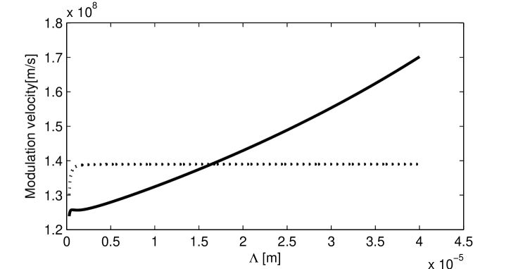
Figure 1: Variations of $\mathrm{v_{modulation}=\Delta\omega/\mid\Delta k\mid}$ (solid line) and velocity of moving $\mathrm{\chi^{(2)}}$, $\mathrm{(v=c/n(\Omega)cos(\theta))}$ (dashed line) versus $\mathrm{\Lambda}$ for $\mathrm{\theta=25}$.

Figure 2: Variations of $\mathrm{v_{modulation}=\Delta\omega/\mid\Delta k\mid}$ (solid line) and velocity of moving $\mathrm{\chi^{(2)}}$, $\mathrm{(v=c/n(\Omega)cos(\theta))}$ (dashed line) versus $\mathrm{\Lambda}$ for $\mathrm{\theta=35}$.

Figure 3: Variations of $\theta$ versus $\Lambda$, which pairs of them are satisfied in the spatiotemporal QPM condition.

Figure 4: (a)The electric field profiles of seed (blue)=$10^{10}$ V/m and pump (red)=$5\times 10^{8}$ V/m and (b) The seed electric field spectrum for $\mathrm{\theta=25}$, after propagating $\mathrm{1.2mm}$. We clearly see the fundamental frequency ($\mathrm{\omega_{0}=1.14\times 10^{15}s^{-1}}$) to the left and its second harmonic (that is seen at $\mathrm{\omega_{2}=2\omega_{0}\mp\Delta\omega}$ not exactly at 2$\omega_{0}$) to the right.

Figure 5: (a)The electric field profiles of seed $(blue)=10^{10}$ V/m and pump (red)=$5\times 10^{8}$ V/m and (b) The seed electric field spectrum for $\mathrm{\theta=35}$, after propagating $\mathrm{1.2mm}$. We clearly see the fundamental frequency ($\mathrm{\omega_{0}=1.14\times 10^{15}s^{-1}}$) to the left and its second harmonic (that is seen at $\mathrm{\omega_{2}=2\omega_{0}\mp\Delta\omega}$ not exactly at 2$\omega_{0}$) to the right.

Figure 6: conversion of energy from the fundamental to the shifted second harmonic $\mathrm{\omega_{2}}$ for $\mathrm{\theta=25}$. The small step-like features on the plot, are characteristic of QPM.

Figure 7: conversion of energy from the fundamental to the shifted second harmonic $\mathrm{\omega_{2}}$ for $\mathrm{\theta=35}$. The small step-like features on the plot, are characteristic of QPM.

References

[1]
M. Conforti, A. Marini, D. Faccio and F. Biancalana, Opt. Express,
21 (2013) 31239.
[2]
D. Faccio, Contemp. Phys., 53 (2012) 97.
[3]
E. Rubino, A. Lotti, F. Belgiorno, S.L. Cacciatori, A. Couairon, U.
Leonhardt and D. Faccio, Scient. Rep., 2 (2012) 932.
[4]
F. Dalla Piazza, F. Belgiorno, S.L. Cacciatori and D. Faccio, Phys.
Rev. A, 85 (2012) 033833.
[5]
F. Belgiorno, S.L. Cacciatori, G. Ortenzi, V.G. Sala and D. Faccio,
Phys. Rev. Lett., 104 (2010) 140403.
[6]
M. Conforti, N. Westerberg, F. Baronio, S. Trillo and D. Faccio,
Phys. Rev. A, 88 (2013) 013829.
[7]
S.C. Kehr, F. Belgiorno, D. Townsend, S. Rohr, C.E. Kuklewicz, U.
Leonhardt, F. Konig and D. Faccio, Phys. Rev. Lett., 108 (2012)
253901.
[8]
J. C. A. Tyrrell , P. Kinsler and G. H. C. New, J. Modern Optics, 52
(2005) 973.
[9]
R.M. Joseph and A. Taflove, IEEE Trans. Antennas Propagat., 45
(1997) 364.
[10]
T. Lee and S.C. Hagness, J. Opt. Soc. Am. B, 21 (2004) 300.
[12]
R. Dworczak and D. Kieslingerb, Phys. Chem. Chem. Phys., 2 (2000)
5057.
[13]
F. Trojanek, K.Zidek, B. Dzurnak, M. Kozak, and P. Maly, Opt.
Express, 18 (2010) 1349.
[14]
A. Bahabad, M. M. Murnane and H. C. Kapteyn, Nature Photonics, 4
(2010) 571.