Fast Computation on Semirings Isomorphic to $(\times,\max)$ on $\mathbb{R}_{+}$

Abstract

Important problems across multiple disciplines involve computations on the semiring $(\times,\max)$ (or its equivalents, the negated version $(\times,\min)$), the log-transformed version $(+,\max)$, or the negated log-transformed version $(+,\min)$): max-convolution, all-pairs shortest paths in a weighted graph, and finding the largest $k$ values in $x_{i}+y_{j}$ for two lists $x$ and $y$. However, fast algorithms such as those enabling FFT convolution, sub-cubic matrix multiplication, etc., require inverse operations, and thus cannot be computed on semirings. This manuscript generalizes recent advances on max-convolution: in this approach a small family of $p$-norm rings are used to efficiently approximate results on a nonnegative semiring. The general approach can be used to easily compute sub-cubic estimates of the all-pairs shortest paths in a graph with nonnegative edge weights and sub-quadratic estimates of the top $k$ values in $x_{i}+y_{j}$ when $x$ and $y$ are nonnegative. These methods are fast in practice and can benefit from coarse-grained parallelization.

1 Introduction

Rings are algebraic structures in which two operations $(\otimes,\oplus)$, generalizations of the standard $\times$ and $+$, are supported, and where the outcomes of the operations must be found in the set of interest (e.g., the ring $(\times,+)$ on the set of integers states that adding or multiplying any two integers must yield an integer). Importantly, the operations $\otimes$ and $\oplus$ must be invertible: for $x$ and $y$ in the ring, $z=x\oplus y$ must be invertible to produce either $x$ (which can be recovered as $z\oplus-y$) or $y$ (which can be recovered as $z\oplus-x$) again (the same is true for the operation $\times$, except the case when $x\otimes y=0$). The more general semirings do not necessarily include this inverse operation. For example, on the semiring $(+,\max)$, given only $z=\max(x,y)$ and the value of $y$, it is not possible to retrieve the value of $x$. The greater generality of semirings makes them important in geometry, optimization, and physics Golan (2013).

The seemingly pedantic distinction between semirings and rings becomes more pronounced when considering certain fast algorithms, which can be applied on rings but not on semirings. A key example of this is fast convolution with the fast Fourier transform (FFT). On the ring $(\times,+)$, FFT can be used to perform convolution in $O(n\log(n))$ steps (superior to the $O(n^{2})$ required by a naive convolution algorithm); however, one of the keys to the feasibility of FFT convolution is the notion that the polynomial coefficients can be combined into a point representation of the polynomials, which is then operated upon, and then un-combined into the coefficients of the product polynomial (essentially, operating on them while combined saves substantial time). For this reason, faster-than-naive algorithms for performing “standard” convolution (i.e., convolution on the ring $(\times,+)$) are very well established numerical methods Cooley and Tukey (1965), whereas the first algorithm with worst-case runtime in $o(n^{2})$ for max-convolution (i.e., convolution on the semiring $(\times,\max)$ Bussieck et al. (1994)) was published fairly recently Bremner et al. (2006) and considered by many, including myself, to be a significant breakthrough. However, this sub-quadratic max-convolution algorithm has a runtime that is only slightly lower than quadratic when compared to the $O(n\log(n))$ fast standard convolution methods mentioned above. The development of fast algorithms for max-convolution is considered important, because FFT convolution-based dynamic programming algorithms can be used to perform fast sum-product statistical inference on sums of two or more random variables Tarlow et al. (2012); Serang (2014), but when performing max-product (i.e., maximum a posteriori) inference (i.e., computing the best configuration) the resulting problem is a max convolution, which was previously limited to algorithms significantly slower than FFT Serang (2015) (with the exception of the binary case $n=2$, wherein an $O(n\log(n))$ maximum a posteriori algorithm based on sorting is possible Tarlow et al. (2010)).

Reminiscent of the disparity between convolution over rings and convolution over semirings is the disparity between matrix multiplication over rings versus matrix multiplication over semirings: Where naive matrix multiplication is in $O(n^{3})$, fast matrix multiplication once again performs operations on combined elements and then un-combines them to achieve a runtime in $O(n^{2.807})$ with Strassen’s algorithm Strassen (1969), which has since been improved by other algorithms with the same strategy, such as with the $O(n^{2.375})$ Coppersmith-Winograd algorithm Coppersmith and Winograd (1987), as well as newer variants of improved worst-case runtime Williams (2012); Le Gall (2014). However, the use of that un-combine step (i.e., inverting the $\oplus$ operation in this case) in the faster-than-naive algorithms prevents using such algorithms on semirings. For example, given an adjacency matrix corresponding to some graph, matrix multiplications on the semiring $(+,min)$ can be used to perform edge relaxations and find the shortest paths between any two vertices in the graph. This was initially conceived as a manner of multiplying the adjacency matrix by itself on the semiring $(+,\min)$ to relax edges (i.e., when the path $u\rightarrow x\rightarrow v$ is more efficient than the direct edge $u\rightarrow v$, using $u\rightarrow x\rightarrow v$ as the new best distance, which replaces the direct edge), thereby making a new adjacency matrix containing all paths of length $\leq 2$. This process could be repeated, with $n-1$ matrix multiplications on the semiring $(+,\min)$, thereby yielding all most efficient paths of length $\leq n$ (equivalent to the most efficient paths overall, since no optimal path would be longer then $n$ edges when each edge weight is in $\mathbb{R}_{+}$), resulting in an algorithm that runs in $O(n^{4})$ Shimbel (1953). From there it is trivial to achieve a speedup by computing the iterative matrix multiplication via the powers of two:

$$A^{n}=\begin{cases}{(A^{2})}^{\frac{n}{2}}&n~{}(\mbox{mod}~{}2)=0\\ A\times{(A^{2})}^{\frac{n-1}{2}}&else.\\ \end{cases}$$

Matrix multiplication over the semiring $(+,\min)$ solves the all-pairs shortest paths problem (APSP) in $\log(n)$ matrix multiplications (or $O(n^{3}\log(n))$ time); however, existing fast matrix multiplication methods cannot be applied to the $(+,\min)$ semiring, and thus speedups substantially below $O(n^{3})$ (the runtime required to solve the APSP problem with the Floyd-Warshall algorithm Floyd (1962); Warshall (1962)) are not achieved by simply utilizing fast matrix multiplication. In fact, it has been proven that restricting the available operations to $+$ and $<$, implies $\Omega(n^{3})$ such operations are necessary to solve the problem exactly Kerb (1970); Williams (2014). The APSP problem is crucially important to many different fields, including applications where the connection to APSP is trivial (e.g., GPS driving directions, routing network traffic) and applications where the connection to APSP is nontrivial (e.g., a fast APSP solution being used within the sub-quadratic max-convolution algorithm of  Bremner et al. (2006)). Research has focused primarily on exploiting properties of particular graphs (e.g., using the fact that its adjacency matrix is sparse, that the graph is planar, etc.), or in more general cases, approaching the problem in a more combinatorial manner Aingworth et al. (1999); Williams (2014).

Similar to the APSP problem, the problem of sorting all $x_{i}+y_{j}$ pairs from lists $x$ and $y$ Fredman (1976) exhibits a combinatorial nature similar to the max-convolution and APSP problems; indeed, one method for performing max-convolution is to compute the top $k$ values in $x^{\prime}_{i}\times y^{\prime}_{j}$ (where $x^{\prime}_{i}=e^{x_{i}}$ and $y^{\prime}_{j}=e^{y_{j}}$) and then fill them in the appropriate indices $m=i+j$ in the max-convolution. However, despite its similarities to the two other problems, this particular problem poses a less clear parallel example where a fast algorithm is available for rings (rather than semirings). All known exact approaches for this problem are in $O(n^{2}\log(n))$, the same as the cost of the naive algorithm (which computes and sorts pairs) Erickson (1997). But the variant where only the top $k$ values are of interest is more complicated, since the top value is trivial (it is the maximum element in $x$ plus the maximum element in $y$) and since the indices considered grow rapidly as $k$ increases: If the lists are first ordered so that $x_{0}\geq x_{1}\geq x_{2}\geq\cdots\geq x_{n-1}$ and $y_{0}\geq y_{1}\geq y_{2}\geq\cdots\geq y_{n-1}$, then $x_{0}+y_{0}$ achieves the maximum, but either $x_{0}+y_{1}$ or $x_{1}+y_{0}$ achieves the second highest, and the third highest will be in $\{x_{0}+y_{1},x_{1}+y_{0},x_{0}+y_{2},x_{2}+x_{0}\}$. Clearly, the values considered by this scheme grow in a combinatorial manner.

This paper draws upon recent work by which fast ring-based algorithms (i.e., algorithms that are only appropriate for use on rings) are used to approximate results on semirings (to which those fast algorithms cannot be applied) via $p$-norm rings, a strategy previously outlined for the max-convolution problem. As noted above, until recently no known algorithms for max-convolution were even remotely as fast as FFT convolution in practice. Here, the method for achieving a numerical estimate of the max-convolution in $O(n\log(n))$ time Serang (2015); Pfeuffer and Serang (2016), is reviewed. The exact max-convolution between two vectors $x$ and $y$ is defined as follows:

$$z = x~{}*_{\max}~{}y$$

$$z_{m} = {(x~{}*_{\max}~{}y)}_{m}$$

$$= \max_{i}~{}x_{i}~{}y_{m-i}$$

$$= \max_{i}~{}u^{(m)}_{i},$$

where $u^{(m)}$ is a vector defined such that $u^{(m)}_{i}=x_{i}~{}y_{m-i}$. Thus, it is possible to see the problem by first filling in lists $u^{(0)}=(x_{0}\times y_{0}),~{}u^{(1)}=(x_{0}\times y_{1},x_{1}\times y_{0}),\ldots~{}u^{(m)}=(x_{0}\times y_{m},x_{1}\times y_{m-1},\ldots~{}x_{m}\times y_{0}),~{}\ldots$, and then the max-convolution result (denoted $z$ above) at index $m$ will be the maximum value found in list $u^{(m)}$. Of course, as described in this naive formulation, the runtime is still quadratic; however it was previously noted that when the elements of $x$ and $y$ are nonnegative, the maximum over each vector $u^{(m)}$ could be found by exploiting the equivalence between the maximum and the Chebyshev norm $\|\cdot\|_{\infty}$, and then using that to numerically approximate the Chebyshev norm with a $p^{*}$-norm, where $p^{*}$ is a large numerical value:

$$\max_{i}~{}u^{(m)}_{i} = \|u^{(m)}\|_{\infty}$$

$$= \lim_{p\to\infty}{\left(\sum_{i}{\left(u^{(m)}_{i}\right)}^{p}\right)}^{\frac{1}{p}}$$

$$\approx {\left(\sum_{i}{\left(u^{(m)}_{i}\right)}^{p^{*}}\right)}^{\frac{1}{p^{*}}},$$

when $p^{*}\gg 1$ Serang (2015). When using a fixed value of $p^{*}$, $u^{(m)}$ can be expanded back into its constituent pieces

$${\left(\sum_{i}{\left(u^{(m)}_{i}\right)}^{p^{*}}\right)}^{\frac{1}{p^{*}}} = {\left(\sum_{i}x_{m}^{p^{*}}~{}y_{m-i}^{p^{*}}\right)}^{\frac{1}{p^{*}}}$$

$$= {\left(x^{p^{*}}~{}*~{}y^{p^{*}}\right)}_{m}^{\frac{1}{p^{*}}}.$$

Thus, it is apparent that the max-convolution can be performed by taking every element of $x_{i}$ to the $p^{*}$ and taking every $y_{i}$ to the $p^{*}$, convolving them regularly (in $n\log(n)$ time using FFT convolution), and then taking every element in that convolution result to the power $\frac{1}{p^{*}}$. Thus, a fast approximation of max-convolution is computed in $n\log(n)$ time (and with a very fast runtime constant, because the algorithm can make use of efficient existing FFT libraries).

Because of numerical instability when $p^{*}\gg 1$ (which is limited to underflow if the input problem is scaled so that all $x_{i}\in[0,1]$ and $y_{i}\in[0,1]$), a piecewise approach that considered $p^{*}\in P\{1,2,4,8,\ldots p^{*}_{\max}\}$ was used, and the highest numerically stable value of $p^{*}$ is used at each index. This is accomplished by computing a single FFT-based max-convolution for each $p^{*}$ and then at each index $m$ in the result, finding the highest $p^{*}$ that produces a result at that index where ${\left(x^{p^{*}}~{}*~{}y^{p^{*}}\right)}_{m}\geq\tau$ (where $\tau$ is the error threshold for the convolution algorithm). Because $\|u^{(m)}\|_{p^{*}}$ is an upper bound of $\|u^{(m)}\|_{\infty}$, when ${\|u^{(m)}\|}^{p^{*}}_{p^{*}}\geq\tau$, then ${\|u^{(m)}\|}^{p^{*}}_{\infty}\geq\tau$, and thus the algorithm does not suffer critical underflow Pfeuffer and Serang (2016). This achieves a stable estimate with bounded error when $p^{*}_{\max}\in O(\log(n))$, and thus the full procedure (over all $p^{*}$ considered) can be performed in $O(n\log(n)\log(\log(n)))$.

When the inputs are $\in[0,1]$, the worst-case relative error has been bounded Pfeuffer and Serang (2016):

$$\frac{|\|u^{(m)}\|_{p^{*}}-\|u^{(m)}\|_{\infty}|}{\|u^{(m)}\|_{\infty}} = \frac{\|u^{(m)}\|_{p^{*}}-\|u^{(m)}\|_{\infty}}{\|u^{(m)}\|_{\infty}}$$

$$= \frac{\|u^{(m)}\|_{p^{*}}}{\|u^{(m)}\|_{\infty}}-1$$

$$\leq n^{\frac{1}{p^{*}}}-1,$$

where $p^{*}$ is the largest $p^{*}\in P$ that produces a numerically stable result. By dividing the estimate by the maximum possible value of $\frac{\|u^{(m)}\|_{p^{*}}}{\|u^{(m)}\|_{\infty}}$, (i.e., dividing by $n^{\frac{1}{p^{*}}}$) the worst-case relative error can be decreased to $|n^{\frac{-1}{p^{*}}}-1|=1-n^{\frac{-1}{p^{*}}}$.

But even more significantly, rather than simply use $\|u^{(m)}\|_{p^{*}}$ to approximate the maximum,  Pfeuffer and Serang (2016) also proposed a method for using the shape of the $p^{*}$ vs. $\|u^{(m)}\|_{p^{*}}$ curve to estimate $\|u^{(m)}\|_{\infty}$. There are multiple ways to estimate $\|u^{(m)}\|_{\infty}$ from this curve, but one way that achieves a good balance between accuracy and efficiency is to model the norm sequence by representing the unique elements in $u^{(m)}$ as a multiset and then projecting down to a smaller number of elements:

$$\|u^{(m)}\|_{p^{*}}^{p^{*}} = \sum_{i}{u^{(m)}_{i}}^{p^{*}}$$

$$= \sum_{j}^{e_{m}}h_{j}{\beta_{j}}^{p^{*}},$$

where each $\beta_{j}$ is one of the $e_{m}$ unique values in $u^{(m)}$ and $h_{j}$ is the number of occurences of $\beta_{j}$. From this perspective, it is possible to use empirically observed values of $\|u^{(m)}\|_{p^{*}}$ (for a few different $p^{*}\in P$) and then project the $e_{m}$ unique $\beta_{j}$ values and their respective counts $h_{j}$ down to a smaller number of $r\leq e_{m}$ unique $\alpha_{j}$ values and their respective counts $n_{j}$:

$$\|u^{(m)}\|_{p^{*}}^{p^{*}} \approx \sum_{j}^{r}n_{j}{\alpha_{j}}^{p^{*}}.$$

Given $2r$ norms from evenly spaced norms $\|u^{(m)}\|_{p^{*}},\|u^{(m)}\|_{2p^{*}},\|u^{(m)}\|_{3p^{*}},\ldots$, the projection onto $r$ unique values $\alpha_{1},\alpha_{2},\ldots\alpha_{r}$ has been shown to be zeros of the polynomial

$$\forall j,~{}\sum_{i=0}^{r}\gamma_{i}\alpha_{j}^{ip^{*}}=0$$

(these zeros can be found by solving for the roots of the polynomial $\sum_{i=0}^{r}\gamma_{i}a^{i}$ and then taking each root to the power $\frac{1}{p^{*}}$), where $\gamma_{0},\gamma_{1},\ldots\gamma_{r}$, the coefficients of the polynomial, are defined by

$$\left[\begin{array}[]{c}\gamma_{0}\\ \gamma_{1}\\ \gamma_{2}\\ \vdots\\ \gamma_{r}\end{array}\right]\in null\left(\left[\begin{array}[]{ccccc}\|u^{(m)}\|_{p^{*}}^{p^{*}}&\|u^{(m)}\|_{2{p^{*}}}^{2{p^{*}}}&\|u^{(m)}\|_{3{p^{*}}}^{3{p^{*}}}&\cdots&\|u^{(m)}\|_{(r+1){p^{*}}}^{(r+1){p^{*}}}\\ \|u^{(m)}\|_{2{p^{*}}}^{2{p^{*}}}&\|u^{(m)}\|_{3{p^{*}}}^{3{p^{*}}}&\|u^{(m)}\|_{4{p^{*}}}^{4{p^{*}}}&\cdots&\|u^{(m)}\|_{(r+2){p^{*}}}^{(r+2){p^{*}}}\\ \|u^{(m)}\|_{3{p^{*}}}^{3{p^{*}}}&\|u^{(m)}\|_{4{p^{*}}}^{4{p^{*}}}&\|u^{(m)}\|_{5{p^{*}}}^{5{p^{*}}}&\cdots&\|u^{(m)}\|_{(r+3){p^{*}}}^{(r+3){p^{*}}}\\ \vdots&\vdots&\vdots&&\vdots\\ \|u^{(m)}\|_{(r){p^{*}}}^{(r){p^{*}}}&\|u^{(m)}\|_{(r+1){p^{*}}}^{(r+1){p^{*}}}&\|u^{(m)}\|_{(r+2){p^{*}}}^{(r+2){p^{*}}}&\cdots&\|u^{(m)}\|_{2r{p^{*}}}^{2r{p^{*}}}\\ \end{array}\right]\right).$$

The maximum value in $u^{(m)}$ can thus be estimated as $\max\{\alpha_{1},\alpha_{2},\ldots\alpha_{r}\}$.

When $r=1$, this projection will be of the form

$$\|u^{(m)}\|_{\infty} \approx {\left(\frac{\|u^{(m)}\|_{p^{*}}}{\|u^{(m)}\|_{\frac{p^{*}}{2}}}\right)}^{\frac{1}{p^{*}}}$$

$$= {\left(\|u^{(m)}\|_{\infty}\frac{\|v\|^{2}_{2}}{\|v\|_{1}}\right)}^{\frac{1}{p^{*}}},$$

for some vector $v$ with elements in $[0,1]$ and where at least one element equals $1$ (w.l.o.g., let $v_{1}=1$). Therefore, the worst-case relative error takes the form

$$1-{\left(\frac{\|v\|_{2}^{2}}{\|v\|_{1}}\right)}^{\frac{1}{p^{*}}}$$

and will be maximized when the estimate ${\left(\frac{\|v\|_{2}^{2}}{\|v\|_{1}}\right)}^{\frac{1}{p^{*}}}$ attains a minimum, which corresponds to minimizing $\frac{\|v\|_{2}^{2}}{\|v\|_{1}}$. Aside from boundary points on the $[0,1]$ hypercube, those extrema will occur when

$$\nabla\frac{\|v\|_{2}^{2}}{\|v\|_{1}}=0$$

or equivalently,

$$\forall i>1,~{}\frac{\left(\frac{\partial}{\partial v_{i}}\|v\|_{2}^{2}\right)\|v\|_{1}-\left(\frac{\partial}{\partial v_{i}}\|v\|_{1}\right)\|v\|_{2}^{2}}{{\|v\|}^{2}}=0.$$

Because $v\succeq 0$ and $v_{1}=1$, then the denominator ${\|v\|}^{2}>0$, and it is therefore possible to exploit symmetry between the equations from two different partial derivatives $j\neq i$ (where neither $i$ nor $j$ is $1$, because $v_{1}=1$ is now a constant):

$$\frac{\left(\frac{\partial}{\partial v_{i}}\|v\|_{2}^{2}\right)\|v\|_{1}-\left(\frac{\partial}{\partial v_{i}}\|v\|_{1}\right)\|v\|_{2}^{2}}{{\|v\|}^{2}} = \frac{\left(\frac{\partial}{\partial v_{i}}\|v\|_{2}^{2}\right)\|v\|_{1}-\left(\frac{\partial}{\partial v_{i}}\|v\|_{1}\right)\|v\|_{2}^{2}}{{\|v\|}^{2}}$$

$$\left(\frac{\partial}{\partial v_{i}}\|v\|_{2}^{2}\right)\|v\|_{1}-\left(\frac{\partial}{\partial v_{i}}\|v\|_{1}\right)\|v\|_{2}^{2} = \left(\frac{\partial}{\partial v_{i}}\|v\|_{2}^{2}\right)\|v\|_{1}-\left(\frac{\partial}{\partial v_{i}}\|v\|_{1}\right)\|v\|_{2}^{2}$$

$$2v_{i}\|v\|_{1}-\|v\|_{2}^{2} = 2v_{j}\|v\|_{1}-\|v\|_{2}^{2}$$

$$v_{i} = v_{j}.$$

Therefore, a critical point for $v$ contains at most two unique values (including $v_{1}=1$). The value $\frac{\|v\|_{2}^{2}}{\|v\|_{1}}$ takes the form $\frac{1+(n-1)\lambda^{2}}{1+(n-1)\lambda}$. The extrema can now be found by optimizing with respect to $\lambda$, which yields $\lambda=\frac{\sqrt{n}-1}{n-1}$, for which $\frac{\|v\|_{2}^{2}}{\|v\|_{1}}=2\frac{\sqrt{n}-1}{n-1}$. Therefore, the worst-case relative error with the $r=1$ projection is bounded by ${\left(2\frac{\sqrt{n}-1}{n-1}\right)}^{\frac{1}{p^{*}}}$.

With $r=2$, the projection likewise has a closed form (described by Pfeuffer and Serang (2016)), and empirical evidence suggests that the worst-case error will be achieved with three unique values in $u^{(m)}$ (meaning there will likewise be three unique values in $v$, including $v_{1}=1$). Although the ability to achieve the worst-case error for $r=2$ projection using three unique values has not been proven, if it were true, it would imply that the worst-case relative error for the $r=2$ projection is $<1-{0.7}^{\frac{4}{p^{*}}}$, meaning that it no longer depends on $n$.

Essentially the projection methods use the shape of the $p^{*}$ vs. $\|u^{(m)}\|_{p^{*}}$ curve to estimate the maximum value in $u^{(m)}$. Furthermore, when only a constant number of $p^{*}$ are considered ($|P|\in O(1)$), numerical max-convolution can be approximated numerically in $O(n\log(n))$ with a practical runtime only slightly slower than standard FFT convolution.

For the sake of simplicity, this manuscript abstracts the projection step into a black box function estimateMaxFromNormPowerSequence, which accepts a spectrum of norms of some vector $u^{(m)}$ and then uses them to estimate the maximum value in $u^{(m)}$.

This manuscript demonstrates that the fast max-convolution method described above generalizes as a strategy for all problems on semirings isomorphic to the semiring $(\times,\max)$ on nonnegative values. By exploiting the fact that a sequence of $(\times,+)$ computations in different $p^{*}$-norms can be used to estimate the results on the semiring $(\times,\max)$, high-quality approximations can be achieved using off-the-shelf fast algorithms limited to rings. In addition to the max-convolution method previously described, the generalized approach is demonstrated on the two other difficult semiring problems: the APSP problem and finding the top $k$ values in $x_{i}+y_{j}$. Using a family of $O(1)$ many $p^{*}$-norms for $p^{*}\in P$, the ring $(\times,+)$ defined for each $p^{*}$-norm can be solved using faster-than-naive algorithms (which can be applied because operations are performed in a $(\times,+)$ ring). Then, for any index in the result, the sequence of results at each $p^{*}$-norm can be used to approximate the $(\times,max)$ semiring. Using this general approach, it is possible to compute a high-quality approximation for the APSP problem in sub-cubic time and compute a high-quality approximation of the top $k$ values in $x_{i}+y_{j}$ (including estimates of their indices $(i,j)$, which cannot be computed by any other known approximation strategies) in $O((n+k)\log(n))$.

2 Methods

2.1 A General Approach to Adapting Fast Algorithms to Nonnegative Semirings

The outline of the approach presented here is as follows: $F$ is a naive algorithm of interest that inefficiently solves a problem on the semiring $(\times,\max)$. $G$ is an identical algorithm on the ring $(\times,+)$. $H$ is an algorithm that produces an equivalent result to $G$, but does so in a faster manner (e.g., FFT convolution, Strassen matrix multiplication, etc.). It is then demonstrated that, for a family of $p^{*}$ values, $G$ can be used to compute a sequence of $p^{*}$-norms, which can be used to approximate $F$. The same approximation can therefore be achieved using $H$ instead of $G$, since $H$ exhibits identical behavior to $G$ (even if it internally performs computations in a manner completely different from $G$).

The semiring of interest defines $(\times,\max)$ on the real numbers. Let $I$ be a collection of nonnegative real-valued inputs. Let $F$ be a finite sequence of operations from the semiring of interest (i.e., $\max$ and $\times$ operations) on the values in collection $I$, which returns a new collection of those results $F(I)$. Let $G$ be a finite sequence of operations created by replacing every $\max$ operation in $F$ with a $+$ operation. Where calling $F(I)$ returned some collection, now $G(I)$ will return a collection of identical shape (i.e., the return values can be thought of as tensors of the same dimension and shape). Let $H$ be a finite sequence of operations where, for every valid input $I$, $H(I)$ returns a result numerically indistinguishable to calling $G(I)$. Because many fast algorithms used for $H$ will have less numerical stability than their naive counterparts, stipulate that $H(I)_{j}\approx G(I)_{j}$ (i.e., the result value at some index $j$ of the result tensor is numerically indistinguishable) whenever the result $H(I)_{j}$ has experienced neither critical underflow nor overflow. In summary, stipulate that $H(I)_{j}\approx G(I)_{j}$ whenever $H(I)_{j}$ approaches neither zero nor infinity. If the means by which overflow occurs is limited (this is achieved by scaling the inputs in $[0,1]$, described later in this manuscript), then it is sufficient to stipulate that $H(I)_{j}$ is accurate when sufficiently greater than zero. In other words, ${G(I)}_{j}\approx{H(I)}_{j}$ when ${H(I)}_{j}\geq\tau$, where $\tau$ is a value that depends on the numeric stability of $H$.

Now consider that any sequence of operations creating an expression in $F$ can be distributed and rearranged into an equivalent expression: $a\times\max\{c,d\}=\max\{a\times c,a\times d\}$. Therefore, any of the results computed by $F$ must be of the form $F(I)_{j}=\max\{\alpha_{1},\alpha_{2},\alpha_{3},\ldots\}$, where the $\alpha_{i}$ values are the results of finite numbers of products of the inputs. Note that the ring $(\times,+)$ possesses a similar property: $a\times(b+c)=(a\times b)+(a\times c)$, implying any results from $G$ or $H$ will be equal to an expression of the form $H(I)_{j}\approx G(I)_{j}=\alpha_{1}+\alpha_{2}+\alpha_{3}+\cdots$ where the $\alpha_{i}$ values are the result of finite numbers of products on the inputs. Because the $\alpha_{1},\alpha_{2},\ldots$ values are products of combinations of the inputs, then calling $H(I^{p^{*}})$ (where $I^{p^{*}}$ denotes taking each element of $I$ to the power $p^{*}$) will produce results of the form $H(I^{p^{*}})_{j}=\alpha_{1}^{p^{*}}+\alpha_{2}^{p^{*}}+\alpha_{3}^{p^{*}}\cdots$, because ${x_{1}}^{p^{*}}\times{x_{2}}^{p^{*}}\times\cdots={\left(x_{1}\times x_{2}\times\cdots\right)}^{p^{*}}$.

When taking the input values to large powers $p^{*}$, values larger than $1$ quickly become large and values smaller than $1$ quickly approach zero. For this reason, let

$$H^{\prime}(I,p^{*})=H\left({\left(\frac{I}{\max_{i}~{}I_{i}}\right)}^{p^{*}}\right)\times\max_{i}~{}I_{i}~{}.$$

Then the error directly introduced by moving to the $p^{*}$-norm ring will be limited to underflow, since all inputs will be scaled to values in $[0,1]$. For any given result at index $j$, values of $p^{*}$ that result in critical levels of underflow will be excluded by verifying that $H^{\prime}(I,p^{*})_{j}\geq\tau$. Because overflow is no longer considered at index $j$, and because critical underflow has been ruled out by the definitions of $H$ and $\tau$ chosen above, then it follows that $G(I^{p^{*}})_{j}\approx H^{\prime}(I,p^{*})_{j}$. For example, when using a high-quality FFT library for fast convolution of vectors with elements in $[0,1]$ and of length $n$ (where $n$ is small enough to permit storing the vectors in RAM on current computers), a result value at some index $j$ where FFT convolution is greater than roughly ${10}^{-12}$ indicates that FFT convolution was stable to underflow. And since significant overflow cannot have occurred, this result is numerically stable with respect to underflow and overflow, because overflow was eliminated by first scaling the problem Pfeuffer and Serang (2016). So if $G(I)$ performs the naive convolution between two vectors and $H(I)$ performs the FFT convolution between the same vectors, $H(I)_{j}\geq\tau$ at some index $j$ implies that $H(I)_{j}\approx G(I)_{j}$, where $\tau={10}^{-12}$.

First compute $H(I^{p^{*}}),~{}\forall p^{*}\in P$. Then, for any given result index $j$ it is possible to produce points on the curve $\left(p^{*},H^{\prime}(I,p^{*})_{j}\right),~{}\forall p^{*}\in P$. This curve can be thought of as a sequence of $p^{*}$-norms taken to power $p^{*}$, where the point paired with $p^{*}$ is of the form

$$H^{\prime}(I,p^{*})_{j}=\|\left(\alpha_{1},\alpha_{2},\alpha_{3},\ldots\right)\|_{p^{*}}^{p^{*}}.$$

This curve can be used to compute $E_{j}(I)$, a numerical estimate of the true maximum at index $j$. If the vector used to define result $j$ is denoted $u=\left(\alpha_{1},\alpha_{2},\alpha_{3},\ldots\right)$, then

$${F(I)}_{j}=\max_{i}~{}u_{i}\approx\\ E_{j}(I)=\mbox{\bf estimateMaxFromNormPowerSequence}\left((~{}\|u\|_{p^{*}}^{p^{*}}~{}|~{}\forall p^{*}\in P:\|u\|_{p^{*}}^{p^{*}}\geq\tau~{})\right).$$

Using this strategy, a faster-than-naive algorithm $H$ can be called a constant number of times ($|P|\in O(1)$) to approximate $F$. In the case of the fast numerical approach to max-convolution described in section 1, $F$ corresponds to the naive $O(n^{2})$ max-convolution algorithm, which performs precisely the desired operations in the most naive manner on the semiring $(\times,\max)$. $G$ corresponds to a naive $O(n^{2})$ standard convolution algorithm; this naive standard convolution algorithm could be used $|P|$ times to perform the appropriate operations in $L_{p^{*}}$ space $\forall p^{*}\in P$, and those $p^{*}$-norm results can later be aggregated to approximate the exact result from $F$. However, no speedup is achieved when using the algorithm $G$ in this manner; in fact, this process will almost certainly be slower, since the code of $G$ is nearly identical to $F$ and is called a small number of times for the different $p^{*}$ values, whereas $F$ is only called once. In this case, $H$ corresponds to an $O(n\log(n))$ FFT standard convolution algorithm, which is chosen exclusively based on its numerical equivalence to $G$. For this reason, even if the steps in $H$ include operations other than $\times$ or $+$ (such as with FFT convolution), its underlying equivalence to $G$ still affords much more efficient estimation of the various $p^{*}$-norms. These norms can in turn, permit numerical estimation of $F$, even if there is no apparent direct connection between $F$ and $H$.

2.2 Fast Estimation of All-Pairs Shortest Paths Distances

First, the proposed approach is demonstrated on a classic computer science problem, the APSP problem. In the most general case, when the adjacency matrix is dense (i.e., when all pairs of nodes in the graph are joined by an edge), sub-cubic runtimes have been achieved by complicated algorithms. The approach estimates the APSP resultant path lengths in $O(M(n)\log(n))$ steps, where $M(n)$ is the cost of standard floating-point matrix multiplication ($M(n)$ is $O(n^{3})$ with naive matrix multiplication, $O(n^{2.807})$ with Strassen’s multiplication method, $O(n^{2.36})$ with the Coppersmith-Winograd algorithm, etc.). The proposed method can be applied to graphs (or directed graphs) with nonnegative edge weights $W_{u,v}\geq 0,~{}(u,v)\in E$ (i.e., where $W$ describes the adjacency matrix of the graph). The APSP problem seeks to find the shortest path between every pair of vertices: for any two vertices $(u,v)$, the shortest distance computed in the APSP problem would consider all paths from $u$ to $v$ and find the one with shortest distance, including direct paths, paths that pass through a single other vertex $x$, paths that pass through vertices $x$ then $y$, etc.: $\min~{}\{W_{u,v},\min_{x}~{}W_{u,x}+W_{x,v},\min_{x,y}~{}W_{u,x}+W_{x,y}+W_{y,v},\ldots\}$.

Here, the input consists of the collection of weights $I=W$. Define the naive algorithm to iteratively relax edges (i.e., it repeatedly finds shorter edges as it progresses) by performing $\log(n)$ matrix multiplications on the semiring $(+,\min)$. Aside from statically bounded looping instructions (which could be unrolled for any particular problem), each of those matrix multiplications is constructed entirely of operations in the semiring $(+,\min)$. Because the runtime is dominated by the $(+,\min)$ matrix multiplications, it is possible to first simplify by letting $F$ be the naive matrix multiplication routine defined on the semiring (algorithm 1).

On a graph with nonnegative edge weights, it is trivial to create a bijective problem on $(\times,\max)$, by letting $W^{\prime}_{i,j}=e^{-W_{i,j}}$: thus $e^{-\left(W_{i,j}+W_{j,k}\right)}=e^{-W_{i,j}}\times e^{-W_{j,k}}$, indicating that $+$ operations have been converted to $\times$ operations. Likewise, since $e^{-x}$ is a strictly decreasing function on $\mathbb{R}_{+}$, then $\min$ has become $\max$ in the transformed space; an equivalent method $F^{\prime}$ can be made, which operates on the semiring $(\times,\max)$. $F^{\prime}$ is then used to process transformed inputs (algorithm 2). It is now trivial to construct $G$, which performs the same operations as $F$, but where $\max$ (equivalent to $\min$ in the original space) is replaced by $+$ operations (algorithm 3). Lastly, $H$ is constructed as an algorithm numerically equivalent to $G$ that achieves greater speed by using any sub-cubic matrix multiplication algorithm. Therefore, if $H^{\prime}$ is called (i.e., $H$ is called on scaled inputs) using a small collection of $p^{*}$ values, it is possible to create a sequence of norms for each cell $i,j$ in the result, and from that sequence it is possible to estimate the maximal path lengths $E_{i,j}(I)$ on $(\times,\max)$. These estimates can then be transformed back onto $(+,\min)$ by using the inverse transformation $-\log(E_{i,j}(I))\approx F(I)_{i,j}$. From there, it is clear that $H$ can be chosen as any fast matrix multiplication algorithm (to that end, this manuscript uses the $O(n^{2.807})$ Strassen matrix multiplication algorithm, as shown in algorithm 4).

The following strategy for max-matrix multiplication is proposed: First, compute the standard matrix multiplication

$$C^{(p^{*})}=\\ \left[\begin{array}[]{cccc}{\left(X_{0,0}\right)}^{p^{*}}&{\left(X_{0,1}\right)}^{p^{*}}&\cdots&{\left(X_{0,n-1}\right)}^{p^{*}}\\ {\left(X_{1,0}\right)}^{p^{*}}&{\left(X_{1,1}\right)}^{p^{*}}&&{\left(X_{1,n-1}\right)}^{p^{*}}\\ \vdots&&\ddots&\\ {\left(X_{n-1,0}\right)}^{p^{*}}&{\left(X_{n-1,1}\right)}^{p^{*}}&&{\left(X_{n-1,n-1}\right)}^{p^{*}}\\ \end{array}\right]\cdot\\ \left[\begin{array}[]{cccc}{\left(Y_{0,0}\right)}^{p^{*}}&{\left(Y_{0,1}\right)}^{p^{*}}&\cdots&{\left(Y_{0,n-1}\right)}^{p^{*}}\\ {\left(Y_{1,0}\right)}^{p^{*}}&{\left(Y_{1,1}\right)}^{p^{*}}&&{\left(Y_{1,n-1}\right)}^{p^{*}}\\ \vdots&&\ddots&\\ {\left(Y_{n-1,0}\right)}^{p^{*}}&{\left(Y_{n-1,1}\right)}^{p^{*}}&&{\left(Y_{n-1,n-1}\right)}^{p^{*}}\\ \end{array}\right]$$

for each $p^{*}\in P$ (via Strassen’s algorithm or any other fast matrix multiplication defined on the ring $(\times,+)$). Then the estimate of the max-matrix multiplication at index $i,j$ is computed via the sequence made from vector norms to the $p^{*}$:

$$E_{i,j}(I)=\mbox{\bf estimateMaxFromNormPowerSequence}\left((~{}C^{(p^{*})}_{i,j}~{}|~{}\forall p^{*}\in P:\|u\|_{p^{*}}^{p^{*}}\geq\tau~{})\right).$$

The min-matrix multiplication results can be computed by transforming back to the semiring $(+,\min)$, as described above. Thus, by broadcasting into a small number of $L_{p^{*}}$ spaces, it is possible to approximate a single matrix multiplication on the semiring $(+,\min)$ (algorithm 5), and thereby approximate the APSP path lengths in $\log(n)$ fast matrix multiplications. In this case (using Strassen multiplication), the overall runtime achieved is in $O(n^{2.807}\log(n))$, and is faster in practice than the $O(n^{3})$ Floyd-Warshall algorithm. As mentioned above, other fast matrix multiplication algorithms may be used in place of Strassen’s algorithm. For example, the Coppersmith-Winograd algorithm would make the overall runtime $O(n^{2.36}\log(n))$. Ignoring the runtime constants (which, it should be noted, can significantly slow down the more advanced faster-than-naive matrix multiplication algorithms in practice), when $n={10}^{6}$, $n^{3}={10}^{18}$, whereas $n^{2.36}\log(n)=2.88\times{10}^{15}$.

Algorithm 1 $F_{(APSP)}$: Naive matrix multiplication on the semiring $(+,\min)$. The inputs $X$ and $Y$ are both matrices in $\mathbb{R_{+}}^{n\times n}$. The $(+,\min)$ matrix multiplication between $X$ and $Y$ is returned. The algorithm runs in $O(n^{3})$ time.

1:for $i\in\{0,1,\ldots n-1\}$ do

2:    for $j\in\{0,1,\ldots n-1\}$ do

3:         for $k\in\{0,1,\ldots n-1\}$ do

4:             $R_{i,j}\leftarrow\min(R_{i,j},X_{i,k}+Y_{k,j})$

5:         end for

6:    end for

7:end forreturn $R$

Algorithm 2 $F^{\prime}_{(APSP)}$: Naive matrix multiplication on the semiring $(\times,\max)$. The inputs $X^{\prime}$ and $Y^{\prime}$ are both matrices in ${[0,1]}^{n\times n}$. The $(\times,\max)$ matrix multiplication between $X^{\prime}$ and $Y^{\prime}$ is returned in $O(n^{3})$. The algorithm runs in $O(n^{3})$ time.

1:for $i\in\{0,1,\ldots n-1\}$ do

2:    for $j\in\{0,1,\ldots n-1\}$ do

3:         for $k\in\{0,1,\ldots n-1\}$ do

4:             $R_{i,j}\leftarrow\max(R_{i,j},X^{\prime}_{i,k}\times Y^{\prime}_{k,j})$

5:         end for

6:    end for

7:end forreturn $R$

Algorithm 3 $G_{(APSP)}$: Naive matrix multiplication on the ring $(\times,+)$. The inputs $X^{\prime}$ and $Y^{\prime}$ are both matrices in ${[0,1]}^{n\times n}$. The $(\times,+)$ matrix multiplication between $X^{\prime}$ and $Y^{\prime}$ is returned. The algorithm, identical to $F^{\prime}_{(APSP)}$ but with $\max$ operations replaced with $+$ operations, runs in $O(n^{3})$ time.

1:for $i\in\{0,1,\ldots n-1\}$ do

2:     for $j\in\{0,1,\ldots n-1\}$ do

3:         for $k\in\{0,1,\ldots n-1\}$ do

4:              $R_{i,j}\leftarrow R_{i,j}~{}+~{}X^{\prime}_{i,k}\times Y^{\prime}_{k,j}$

5:         end for

6:     end for

7:end forreturn $R$

Algorithm 4 $H_{(APSP)}$: Sub-Cubic Strassen matrix multiplication on the ring $(\times,+)$. The inputs $X^{\prime}$ and $Y^{\prime}$ are both matrices in ${[0,1]}^{n\times n}$. The $(\times,+)$ matrix multiplication between $X^{\prime}$ and $Y^{\prime}$ is returned. The algorithm produces the same result as $G_{(APSP)}$, but in $O(n^{2.807})$ time.

1:$\left[\begin{array}[]{cc}a&b\\ c&d\\ \end{array}\right]\leftarrow X^{\prime}$

2:$\left[\begin{array}[]{cc}e&f\\ g&h\\ \end{array}\right]\leftarrow Y^{\prime}$

3:$p1\leftarrow H_{(APSP)}(a,f-h)$

4:

5:$p2\leftarrow H_{(APSP)}(a+b,h)$

6:

7:$p3\leftarrow H_{(APSP)}(c+d,e)$

8:

9:$p4\leftarrow H_{(APSP)}(d,g-e)$

10:

11:$p5\leftarrow H_{(APSP)}(a+d,e+h)$

12:

13:$p6\leftarrow H_{(APSP)}(b-d,g+h)$

14:

15:$p7\leftarrow H_{(APSP)}(a-c,e+f)$

16:

17:$R\leftarrow\left[\begin{array}[]{cc}p5+p4-p2+p6&p1+p2\\ p3+p4&p1+p5-p3-p7\\ \end{array}\right]$

18:return $R$

Algorithm 5 $E_{(APSP)}$: Sub-Cubic approximate matrix multiplication on the semiring $(\times,\max)$. Inputs $X^{\prime}$ and $Y^{\prime}$ are both matrices in ${[0,1]}^{n\times n}$. The $(\times,+)$ matrix multiplication between $X^{\prime}$ and $Y^{\prime}$ is returned. The algorithm approximates $F^{\prime}_{(APSP)}$ in $O(n^{2.807})$ time.

1:for $p^{*}\in P$ do

2:    for $i\in\{0,1,\ldots n-1\}$ do

3:         for $j\in\{0,1,\ldots n-1\}$ do

4:             $X^{\prime\prime}_{i,j}\leftarrow{\left(X^{\prime}_{i,j}\right)}^{p}{{}^{*}}$

5:             $Y^{\prime\prime}_{i,j}\leftarrow{\left(Y^{\prime}_{i,j}\right)}^{p}{{}^{*}}$ $\triangleright$ (Create $I^{p^{*}}$; to prevent overflow, instead call $H_{(APSP)}^{\prime}(X^{\prime},Y^{\prime},p^{*})$ below)

6:         end for

7:    end for

8:    $H^{(p^{*})}\leftarrow H_{(APSP})(X^{\prime\prime},Y^{\prime\prime})$ $\triangleright$ (Perform fast operations in rings)

9:end for

10:for $i\in\{0,1,\ldots n-1\}$ do

11:    for $j\in\{0,1,\ldots n-1\}$ do

12:         $normPowerSeq\leftarrow~{}(H^{(p^{*})}_{i,j}~{}|~{}\forall p^{*}\in P:H^{(p^{*})}_{i,j}\geq\tau)$

13:         $R_{i,j}\leftarrow\mbox{\bf estimateMaxFromNormPowerSequence}\left(normPowerSeq\right)$ $\triangleright$ (Aggregate results)

14:    end for

15:end forreturn $R$

2.3 Fast Sorting of $x_{i}+y_{j}$

The fast rings approximation is also demonstrated on a second well-known computer science problem: Sorting a list of all pairs $x_{i}+y_{j}$ where $x$ and $y$ are two $n$-length lists, is a classic problem in computer science for which no known algorithms achieve runtime superior to the naive $O(n^{2}\log(n))$ approach; furthermore, this naive $O(n^{2}\log(n))$ approach (algorithm 6) is the fastest known approach that can also give the indices of $x$ and $y$, by generating all tuples of the form $(x_{i}+y_{j},i,j)$ and sorting them lexicographically. Note that sorting all $n^{2}$ pairs $x_{i}+y_{j}$ would require $O(n^{2}\log(n))$ steps and retrieving the top $k$ values from a max-heap would require inserting all $n^{2}$ values and then dequeuing the top $k$ in $O(k\log(n))$ for an overall runtime in $O(n^{2}+k\log(n))$ where $k\leq n^{2}$.

An approximate solution can be achieved by discretizing to integer values and then binning $x$ and $y$ (the binned counts of $x+y$ values can be computed by convolving the binned $x$ and binned $y$ counts with FFT convolution); however, this approximation is sensitive to the discretization precision (in both accuracy and runtime) and yields only the sorted values $x_{i}+y_{j}$ and not the corresponding indices $i,j$ Erickson (1997). Here a novel numerical approximation to sorting $x+y$ is outlined using the strategies above. The proposed method can also be used to estimate the top $k$ values $x_{i}+y_{j}$ as well as estimate the indices $i,j$ that produce them. As before with the APSP problem, it is possible to draw an isomorphism between the semirings $(+,\max)$ and $(\times,\max)$: $x^{\prime}_{i}=e^{x_{i}},y^{\prime}_{j}=e^{y_{j}}$ so that $e^{x_{i}+y_{j}}=e^{x_{i}}\times e^{y_{j}}$, indicating the $+$ operation has been converted to a $\times$ operation.

Due to recent advances mentioned above regarding fast max-convolution, it is tempting to find a similarity; however, max-convolution does not directly solve the top $k$ values in $x^{\prime}_{i}\times y^{\prime}_{j}$: Given $z=x~{}*_{\max}~{}y$ (i.e., the max-convolution between $x$ and $y$) the largest value in the max-convolution must be the largest value in $x^{\prime}_{i}\times y^{\prime}_{j}$: $\max_{m}~{}z_{m}=\max_{i}~{}\max_{j}~{}x^{\prime}_{i}\times y^{\prime}_{j}$. But the second largest value in the max-convolution does not necessarily belong to the top $k$ values of $x^{\prime}_{i}\times y^{\prime}_{j}$, because the max-convolution at index $m$ gives the maximum value over all positive diagonals for which $i+j=m$; if the second largest value in $x^{\prime}_{i}\times y^{\prime}_{j}$ has the same $m=i+j$ value as the first largest value chosen, then it will be obscured by first choice because $z_{m}=\max_{i}~{}u^{(m)}_{i}$, where $u^{(m)}$ is a vector that holds all elements $x^{\prime}_{i}\times y^{\prime}_{j}$ along the positive diagonal $m=i+j$, and $z$ only contains the maximum value of $u^{(m)}$, not the second highest value, third highest value, etc..

It is trivial to see a naive sorting approach that simply performs $\mbox{\bf sort}\left(~{}(x^{\prime}_{0}\times y^{\prime}_{0},x^{\prime}_{0}\times y^{\prime}_{1},x^{\prime}_{0}\times y^{\prime}_{2},\ldots x^{\prime}_{1}\times y^{\prime}_{0},x^{\prime}_{1}\times y^{\prime}_{1},\ldots)~{}\right)$; but this sorting method is already obfuscated by the clever optimizations inherent to $O(n\log(n))$ sorting algorithms. For this reason, a different algorithm $F$ is chosen; this $F$ algorithm is equivalent to sorting all pairs $x^{\prime}_{i}\times y^{\prime}_{j}$, but the chosen definition of $F$ eschews the complexity of sophisticated sorting routines in favor of something simpler, although it is slower than the naive approach of generating all $n^{2}$ $x^{\prime}_{i}\times y^{\prime}_{j}$ pairs and sorting them with an arbitrary $O(n\log(n))$ algorithm. Essentially, the algorithm is equivalent to finding the maximum value along each positive diagonal, and then the maximum value over those maximum values, which gives the next largest value in $x^{\prime}_{i}\times y^{\prime}_{j}$ (algorithm  7). The $u^{(m)}$ vectors correspond to the positive-sloping diagonals in the following matrix:

$$\left[\begin{array}[]{ccccc}x^{\prime}_{0}\times y^{\prime}_{0}&x^{\prime}_{0}\times y^{\prime}_{1}&x^{\prime}_{0}\times y^{\prime}_{2}&&x^{\prime}_{0}\times y^{\prime}_{n-1}\\ x^{\prime}_{1}\times y^{\prime}_{0}&x^{\prime}_{1}\times y^{\prime}_{1}&x^{\prime}_{1}\times y^{\prime}_{2}&\cdots&x^{\prime}_{1}\times y^{\prime}_{n-1}\\ x^{\prime}_{2}\times y^{\prime}_{0}&x^{\prime}_{2}\times y^{\prime}_{1}&x^{\prime}_{2}\times y^{\prime}_{2}&&x^{\prime}_{2}\times y^{\prime}_{n-1}\\ &\vdots&&\ddots\\ x^{\prime}_{n-2}\times y^{\prime}_{0}&x^{\prime}_{n-2}\times y^{\prime}_{1}&x^{\prime}_{n-2}\times y^{\prime}_{2}&&x^{\prime}_{n-2}\times y^{\prime}_{n-1}\\ x^{\prime}_{n-1}\times y^{\prime}_{0}&x^{\prime}_{n-1}\times y^{\prime}_{1}&x^{\prime}_{n-1}\times y^{\prime}_{2}&&x^{\prime}_{n-1}\times y^{\prime}_{n-1}\\ \end{array}\right].$$

And so $u^{(0)}=(x^{\prime}_{0}\times y^{\prime}_{0})$, $u^{(1)}=(x^{\prime}_{1}\times y^{\prime}_{0},x^{\prime}_{0}\times y^{\prime}_{1})$, $u^{(2)}=(x^{\prime}_{2}\times y^{\prime}_{0},x^{\prime}_{1}\times y^{\prime}_{1},x^{\prime}_{0}\times y^{\prime}_{2})$, $\ldots u^{(2n-2)}=(x^{\prime}_{n-1}y^{\prime}_{n-1})$. Once the next highest remaining value is computed, that value is removed from future consideration by executing the line $u^{(m)}.remove(\psi_{m^{*}})$, which traverses through the list $u^{(m)}$ and removes the first value matching $\psi_{m^{*}}$. Overall, this algorithm runs in $O(n^{3})$ steps.

Algorithm 6 $F_{(X+Y)}$: Naive sorting of $x_{i}+y_{j}$. Inputs $x$ and $y$ are lists of length $n$. The return value is a list of the top $k$ values of the form $x_{i}+y_{j}$. The algorithm runs in $O(n^{2}\log(n))$ time and $O(n^{2})$ space, where $k\in\{1,2,\ldots n^{2}\}$.

1:$unsorted\leftarrow(~{})$

2:for $i\in\{0,1,\ldots n-1\}$ do

3:    for $j\in\{0,1,\ldots n-1\}$ do

4:         $unsorted.append(x_{i}+y_{j})$

5:    end for

6:end for

7:$sorted\leftarrow\mbox{\bf sort}(unsorted)$ return $(~{}sorted[0],sorted[1],\ldots sorted[k-1]~{})$

Algorithm 7 $F^{\prime}_{(X^{\prime}\times Y^{\prime})}$: Naive sorting of $x^{\prime}_{i}\times y^{\prime}_{j}$. The inputs are two lists $x^{\prime}$ and $y^{\prime}$ of length $n$. The return value is a list of the top $k$ values of the form $x^{\prime}_{i}\times y^{\prime}_{j}$. The algorithm runs in $O(n^{2}+nk)$ time and $O(n^{2})$ space, where $k\in\{1,2,\ldots n^{2}\}$.

1:for $m\in\{0,1,\ldots n-1\}$ do

2:    $u^{(m)}\leftarrow(x^{\prime}_{m}\times y^{\prime}_{0},x^{\prime}_{m-1}\times y^{\prime}_{1},x^{\prime}_{m-2}\times y^{\prime}_{2},\ldots x^{\prime}_{0}\times y^{\prime}_{m})$

3:    $\psi_{m}\leftarrow\max_{i}~{}u^{(m)}$

4:end for

5:$R\leftarrow(~{})$

6:for $\ell\in\{1,2,\ldots k\}$ do

7:    $m^{*}\leftarrow\operatornamewithlimits{argmax}_{m}\psi_{m}$

8:    $R.append(\psi_{m^{*}})$

9:    $u^{(m^{*})}.remove(\psi_{m^{*}})$ $\triangleright$ (Remove the value from $u^{(m)}$)

10:    $\psi_{m^{*}}\leftarrow\max_{i}~{}u^{(m^{*})}$

11:end forreturn $R$

Next, the algorithm $G$ is created from $F$ (algorithm 8); note that when it is desirable, only a subset of the $\max$ operations may be replaced by $+$ operations. Finally, a novel data structure motivated by this fast rings approximation is created for sequentially approximating and removing a maximum from a collection of norms, the NormQueue. This novel data structure is paired with fast max-convolution to construct the faster-than-naive algorithm $H$. This underscores that it is also possible to perform dynamic programming while in these various $p^{*}$-norm spaces, and therefore use the result of a computation on the semiring $(\times,\max)$ to subsequently alter the program flow.

The NormQueue works as follows: for some vector $u^{(m)}$, assume a collection of norms to the $p^{*}$ is given

$$NQ = \left(NQ_{1},NQ_{2},NQ_{3},\ldots\right)$$

$$= \left(\|u^{(m)}\|_{p^{*}_{1}}^{p^{*}_{1}},\|u^{(m)}\|_{p^{*}_{2}}^{p^{*}_{2}},\|u^{(m)}\|_{p^{*}_{3}}^{p^{*}_{3}},\ldots\right)$$

from which it is possible to estimate the maximum value in $\|u^{(m)}\|_{\infty}\approx\alpha=\mbox{\bf estimateMaxFromNormPowerSequence}(\|u^{(m)}\|_{{p^{*}}_{1}},\|u^{(m)}\|_{{p^{*}}_{2}},\|u^{(m)}\|_{{p^{*}}_{3}},\ldots)$. If the maximum element in $u^{(m)}$ occurred at index $i^{*}=\operatornamewithlimits{argmax}_{i}u^{(m)}_{i}$, then it is now possible to estimate the norms of the vector ${u^{(m)}}^{\prime}=\left(u^{(m)}_{i}|i\neq i^{*}\right)$ by subtracting the estimated maximum $\alpha$ from each norm:

$$NQ^{\prime} = \left(\|{u^{(m)}}^{\prime}\|_{p^{*}_{1}}^{p^{*}_{1}},\|{u^{(m)}}^{\prime}\|_{p^{*}_{2}}^{p^{*}_{2}},\|{u^{(m)}}^{\prime}\|_{p^{*}_{3}}^{p^{*}_{3}},\ldots\right)$$

$$\approx \left(\|u^{(m)}\|_{p^{*}_{1}}^{p^{*}_{1}}-\alpha^{p^{*}_{1}},\|u^{(m)}\|_{p^{*}_{2}}^{p^{*}_{2}}-\alpha^{p^{*}_{2}},\|u^{(m)}\|_{p^{*}_{3}}^{p^{*}_{3}}-\alpha^{p^{*}_{3}},\ldots\right)$$

$$= \left(NQ_{1}-\alpha^{p^{*}_{1}},NQ_{2}-\alpha^{p^{*}_{2}},NQ_{3}-\alpha^{p^{*}_{3}},\ldots\right),$$

proceeding inductively to iteratively estimate the maximum from the collection of norms and then removing the estimated maximum from those norms. Note that the NormQueue can be used with only $O(1)$ norms, leading to approximate results, but an $O(1)$ runtime to pop and reestimate the new max. While this data structure does accumulate error (because small imperfections in early estimates of the maxima may have ripple effects on later estimates), the larger values experience less of this error because they are retrieved first (limiting the ripple effect of errors accumulated to that point) and because the norm sequence best summarizes larger values (they are not the values that endure underflow).

Algorithm 8 $G_{(X^{\prime}\times Y^{\prime})}$: Method on the ring $(\times,+)$, derived from $F^{\prime}_{(X^{\prime}\times Y^{\prime})}$. The inputs are two lists $x^{\prime}$ and $y^{\prime}$ of length $n$. The return value is analogous to the return value of $F^{\prime}_{X\times Y}$, but using the ring $(\times,\max)$. The algorithm runs in $O(n^{2}+nk)$ time and $O(n^{2}+k)$ space.

1:for $m\in\{0,1,\ldots n-1\}$ do

2:    $u^{(m)}\leftarrow(x^{\prime}_{m}+y^{\prime}_{0},x^{\prime}_{m-1}+y^{\prime}_{1},x^{\prime}_{m-2}+y^{\prime}_{2},\ldots x^{\prime}_{0}+y^{\prime}_{m})$

3:    $\sigma_{m}\leftarrow\sum_{i}~{}u^{(m)}$ $\triangleright$ ($\max$ operation replaced with $\sum$)

4:end for

5:$R\leftarrow(~{})$

6:for $j\in\{1,2,\ldots k\}$ do

7:    $m^{*}\leftarrow\operatornamewithlimits{argmax}_{m}\sigma_{m}$

8:    $R.append(\psi_{m^{*}})$

9:    $u^{(m^{*})}.remove(\psi_{m^{*}})$ $\triangleright$ (Remove the value from $u^{(m)}$)

10:    $\sigma_{m^{*}}\leftarrow\max_{i}~{}u^{(m^{*})}$

11:end forreturn $R$

In order to derive some $H_{X^{\prime}\times Y^{\prime}}$ that is equivalent to but more optimized than $G_{X^{\prime}\times Y^{\prime}}$, notice the fact that the $\psi$ vector computed by $G_{X\times Y}$ is equivalent to a standard convolution. One avenue of attack would be to compute $\psi$ for different $p^{*}\in P$ (denoted $\sigma^{(p*)}$), and then aggregate them to approximate the maximum (computed as the initial $\psi_{m}$ by $F_{X^{\prime}\times Y^{\prime}}$). As noted above, the max-convolution will not solve this problem alone, since the max-convolution discards the second-highest value in each $u^{(m)}$ (once again, operations on the semiring lose information in a manner that cannot be undone). However in this case, it is desirable to keep the information in the $p^{*}$-norm, so that the second-highest value in each $u^{(m)}$ leaves some preserved signature. For this reason, the function $H$ is not defined; instead, the $p^{*}$-norm aggregation is performed within the same function $E$; instead of $E$ calling $H$ (as in the case of max-convolution where $H$ is FFT and in max-matrix multiplication where $H$ is Strassen– or some other faster-than-naive– matrix multiplication), here $E_{X^{\prime}\times Y^{\prime}}$ is described ab initio so that $p^{*}$-norm information from the different calls to $H$ can be shared (algorithm 9). By doing so, the method can exploit the fact that if $\sigma^{(p^{*})}=\sum_{i}{\left(u^{(m)}\right)}^{p^{*}}$, and so can recompute which value $\sigma^{(p^{*})}$ would take if its maximum ($\psi_{m^{*}}$) were removed by simply subtracting out the term the maximum would contribute to the norms: $\sum_{i}{\left(u^{(m)}\right)}^{p^{*}}-{\left(\psi_{m^{*}}\right)}^{p^{*}}$. In practice, by using the NormQueue.

Algorithm 9 $E_{(X^{\prime}\times Y^{\prime})}$: Fast approximate sorting of $x^{\prime}_{i}\times y^{\prime}_{j}$ operating on ring $(\times,\max)$. The inputs are two nonnegative lists $x^{\prime}$ and $y^{\prime}$ of length $n$. The return value is an list approximating the top $k$ values of the form $x^{\prime}_{i}\times y^{\prime}_{j}$. The algorithm runs in $O((n+k)\log(n))$ time and $O(n+k)$ space.

1:for $p^{*}\in P$ do

2:    $\sigma^{(p^{*})}\leftarrow(x^{\prime})^{p^{*}}~{}*~{}{y^{\prime}}^{p^{*}}$ $\triangleright$ (Convolve with FFT)

3:end for

4:$q\leftarrow maxHeap()$

5:for $m\in\{0,1,\ldots n-1\}$ do

6:    $\psi_{m}\leftarrow\mbox{\bf estimateMaxFromNormPowerSequence}\left((\sigma^{(p^{*})}_{m}~{}|~{}\forall p^{*}\in P:\sigma^{(p^{*})}_{m}\geq\tau)\right)$

7:    $q.insert((\psi_{m},m))$

8:end for

9:$R\leftarrow(~{})$

10:for $j\in\{1,2,\ldots k\}$ do

11:    $m^{*}\leftarrow q.popMax()$

12:    $R.append(\psi_{m^{*}})$

13:    for $p^{*}\in P$ do

14:         $\sigma^{(p^{*})}_{m}\leftarrow\sigma^{(p^{*})}_{m}-{\left(\psi_{m^{*}}\right)}^{p^{*}}$ $\triangleright$ (Remove the value from $u^{(m)}$)

15:         $\psi_{m^{*}}\leftarrow\mbox{\bf estimateMaxFromNormPowerSequence}\left((\sigma^{(p^{*})}_{m^{*}})~{}|~{}\forall p^{*}\in P:\sigma^{(p^{*})}_{m^{*}}\geq\tau)\right)$

16:    end for

17:end forreturn $R$

Not only does this achieve a very fast approximation of the maximum $k$ values in $x_{i}\times y_{j}$, $E_{X^{\prime}\times Y^{\prime}}$ can be called twice and both calls can be used together to estimate the indices $i,j$ that correspond to each value $x_{i}\times y_{j}$: this is achieved by first noting that $E_{X^{\prime}\times Y^{\prime}}(X^{\prime},Y^{\prime})$ should give the same result regardless of the order of the elements in $Y^{\prime}$. Thus, if $Y^{\prime}[::-1]$ denotes the reverse of $Y^{\prime}$ (Python notation), then $E_{X^{\prime}\times Y^{\prime}}(X^{\prime},Y^{\prime})\approx E_{X^{\prime}\times Y^{\prime}}(X^{\prime},Y^{\prime}[::-1])$. Second, the value $m^{*}$ (i.e., the positive diagonal from which each next value is drawn) can be trivially added to the return value by simply changing the line $result.append(\psi_{m^{*}})$ to $result.append(~{}(\psi_{m^{*}},m^{*})~{})$. Therefore, by computing $E_{X^{\prime}\times Y^{\prime}}(X^{\prime},Y^{\prime})$ and also computing $E_{X^{\prime}\times Y^{\prime}}(X^{\prime},Y^{\prime}[::-1])$, it is possible to get estimates for the positive diagonal from which each element was drawn. Let the positive diagonal for a given result value (from calling $E_{X^{\prime}\times Y^{\prime}}(X^{\prime},Y^{\prime})$) be denoted $m_{1}^{*}=i+j$ and let the negative diagonal from which that same result was drawn (from calling $E_{X^{\prime}\times Y^{\prime}}(X^{\prime},Y^{\prime}[::-1])$) be denoted $m_{2}^{*}=i+(n-1-j)$. It can therefore be seen that $m_{1}^{*}+m_{2}^{*}=2i+n-1$, and so $i=\frac{m_{1}^{*}+m_{2}^{*}-n+1}{2}$. Once $i$ is computed, then $j=m_{1}^{*}-i$. These estimates can subsequently be verified by comparing the approximation $\psi_{m^{*}}$ with the empirical value $x_{i}\times y_{j}$ using the $i,j$ computed above; when both are close, then the $i,j$ value is a reliable estimate. The ability to estimate the indices in this manner is significant, because an existing approximation that creates binned histograms for $X$ and $Y$ and then uses those to compute the binned histogram of $X+Y$ (by convolving the $X$ and $Y$ histograms with FFT) Erickson (1997) cannot be used to estimate indices: doing so would require passing indices through the FFT, which would require a set of integers to be stored for every value in the FFT (rather than a complex floating point value) and those sets will take on several values as the FFT recurses, including the full set $\{0,1,\ldots n\}$. As a result, passing indices through the FFT cannot yet be accomplished in $o(n^{2})$ time.

3 Results

3.1 All-Pairs Shortest Paths in a Weighted Graph

Here an elegant and standard $O(n^{3})$ algorithm, the Floyd-Warshall algorithm, for solving the APSP problem is compared against a simple, novel method that was created using the fast rings approximation strategy. This novel method (made quickly and without a great expertise on the APSP problem) achieves a fairly good approximation and outperforms the Floyd-Warshall algorithm, as shown in table 1. Note that even with a simple and fairly numerically unstable fast matrix multiplication algorithm (a naive implementation of the Strassen algorithm), the approximation is not only close to the exact value, it also often improves as the problem size increases, because there is an increased chance of finding an efficient path between two vertices. The index $(1,0)$ (arbitrarily chosen as the first non-trivial index– index $(0,0)$ necessarily has a distance of $0$) of a single $n=512$ problem yields an exact shortest path distance of $5.1955813$ and an approximate shortest path distance $5.2130877$ (absolute error $<0.01751$).

$n$	16	32	64	128	256	512
Floyd-Warshall runtime	0.01155	0.09297	0.7717	5.956	49.43	378.9
Fast rings approximation runtime	0.02527	0.09537	0.4572	2.594	15.31	103.5
MSE	0.04587	0.05395	0.03049	0.02767	0.02228	0.01207

Table 1: Runtime comparison between Floyd-Warshall and the fast rings approximation method. The practical runtimes of the $O(n^{3})$ Floyd-Warshall algorithm are compared to the proposed $O(M(n)\log(n))$ runtime $p^{*}$-norm rings approximation (in this case, using $p^{*}_{\max}=512$ (i.e., $|P|=18$) and using Strassen matrix multiplication, i.e., $M(n)=O(n^{2.807})$) for problems of various size. For each problem size $n$, $5$ different problems were simulated (by randomly generating adjacency matrices where off-diagonal values were uniformly sampled floating point values $\in[1,100]$). The mean over these $5$ replicates for each $n$ is reported, as well as the mean squared error (MSE) between the exact shortest path weights and the approximate shortest path weights. Note that the speedup grows with $n$. The average square error is $<\pm 0.05$ for all problems considered.

3.2 Sorting $x_{i}+y_{j}$

Here the best known method (which is the naive $O(n^{2}\log(n))$ algorithm) is demonstrated for finding the top $k$ values in $x_{i}+y_{j}$, and compared to a novel $O(n\log(n)+k)$ algorithm based on the fast rings approximation. Once again, the fast rings approximation achieves a superior runtime (figure 1). Although the error is significantly higher in this example (because errors are accumulating in an iterative manner, which is not the case in max-convolution and the APSP problem), not only is the runtime superior, the space requirements are dramatically decreased (from $>14$GB to memory usage in the low MBs due to a linear space requirement), because the matrix of all $x^{\prime}_{i}\times y^{\prime}_{j}$ (or, equivalently, $x_{i}+y_{j}$ in the original, un-transformed space) is never actually computed.

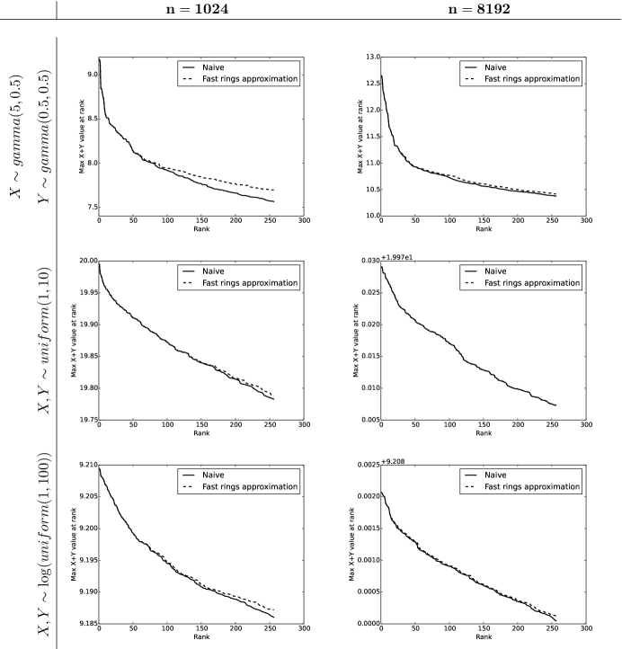
Figure 1: Sorting $x_{i}+y_{j}$. For problems of different size ($n=1024$ and $n=8192$) a single problem (i.e. lists $x$ and $y$) is sampled from various distributions. On each problem, the naive $O(n^{2}\log(n))$ approach is used to sort all possible $n^{2}$ pairs and the top $k=256$ values are compared with the top values estimated with the fast rings approximation in $O(n\log(n))$ time (using $p^{*}_{\max}=4096$, i.e., $|P|=24$). Where the approximation is accurate, the indices $i,j$ that correspond to $x_{i}+y_{j}$ at every rank can be estimated with high fidelity (e.g., all $\frac{256}{256}$ top indices are correct for the uniform distributions with $n=8192$). When $n=8192$, the naive method required $873.2$ seconds and $\approx 15$GB of RAM, while fast approximation requires $0.7209$ seconds and memory usage was insignificant in comparison.

4 Discussion

This manuscript has proposed novel methods for two open problems; although the methods themselves are certainly of interest, most exciting is that both were created without expertise even though both problems (like max-convolution) have been subject to years of hard work by the field. Furthermore, the methods themselves are fairly simple (as was the case for fast max-convolution); other than code for estimateMaxFromNormPowerSequence described in  Pfeuffer and Serang (2016) and implemented in an efficient, vectorized manner with numpy, devising novel approximations is quite simple with this general strategy: just as there are many problems to which this strategy can be applied, there are many other variants of the strategy. The general idea– changing the problem into a spectrum of rings, applying fast algorithms limited to rings, and then estimating the true result from the aggregated spectrum– could also be paired with other soft-max functions that correspond well to the rings.

Even though the APSP approximation only estimates the path weights or distances of the shortest path (as opposed to the path itself), there may be situations where branch and bound can be used to compute the paths in $o(n^{3})$ time given knowledge about the optimal path lengths (i.e., if the final paths are very efficient, then many edges can be excluded wherever the cumulative distance sufficiently exceeds the optimal path distance). Approximation error can even be worked into this scheme by using a small buffer $\delta$ that prevents bounding unless the weight is more than $\delta$ greater than the approximation estimates. Likewise, an approximation may also be suitable for cases from operations research where users are optimizing over graphs, and thus may need to repeatedly estimate the APSP path distances (in this case, it may even be possible to perform local optimizations directly in the $p^{*}$-norm rings, which will be continuous and differentiable). There may also be a strategy similar to how indices can be estimated on the $x_{i}+y_{j}$ problem, which could permit estimation of the destination of each edge taken by matrix multiplication on $(\times,\max)$.

Furthermore, the largest errors appear to occur when the shortest path between two vertices is long; this is because the $(\times,\max)$ variant of the problem operates in a transformed space, and a total path weight of $20$ in the original space $(+,\min)$ corresponds to $e^{-20}$ in the transformed space. For this reason, it is promising to consider the application of scaling to keep the problem in a nicely bounded range or even the possibility of using an alternative transformation and then solving that problem on $(\times,\max)$. In general, it may also be possible to solve $(+,\min)$ problems in a similar manner without transforming to a $(\times,\max)$ formulation.

Considering the $x_{i}+y_{j}$ method, there may be other uses for the NormQueue data structure, the fast, approximate data structure for keeping track of the largest remaining values in a collection based on its norms (rather than storing the values themselves). There may be other applications (e.g., in large-scale databases or web search) where it is possible to cache a small collection of norms (potentially with great efficiency via algorithms like FFT convolution), but where caching the full list would be intractable. Obvious applications would be similar to the $x_{i}+y_{j}$ problem, where a combinatorial effect makes caching results much more difficult, and where algorithms such as FFT convolution can be used to compute the norms on some combination of variables an order of magnitude faster than if the norms were computed from scratch. This sequence of norms can also be updated online in other ways (in addition to the $popMax$ operation employed), such as adding values to the queue (by adding in $x^{p^{*}}$ to the values stored at each $p^{*}$).

Regarding the $x_{i}+y_{j}$ problem itself, it would be very interesting to see if the error of this preliminary algorithm could be improved by performing $E_{X^{\prime}\times Y^{\prime}}(X^{\prime},Y^{\prime})$ and $E_{X^{\prime}\times Y^{\prime}}(X^{\prime},Y^{\prime}[::-1])$ simultaneously (rather than serially, as was used for estimating the indices $i,j$ in this manuscript). If both instances proceed one index at a time, then an estimate of indices $i,j$ could be computed before calling $popMax$; if the estimated indices are accurate, then the exact value $x_{i}+y_{j}$ could replace the estimated value when updating the NormQueue (i.e., when subtracting out the estimated max to the power $p^{*}$ from each $\|u\|^{p^{*}}_{p^{*}}$), and such updates would introduce error much more slowly (because, in an inductive manner, starting with high-quality estimates of the initial maxima would yield to more accurate updating of the NormQueue, which would lead to higher quality estimates of subsequent maxima).

This modularity of this fast rings approximation is a substantial benefit: in the likely case that future research discovers alternative methods for computing estimateMaxFromNormPowerSequence (which in this manuscript uses an $r=2$ projection), the accuracy or the speed-accuracy tradeoff of this method would immediately improve. Future developments in the conjectured error bound for the $r=2$ projections will be of interest, as will error bounds for the $r=3$ and $r=4$ projections, for which closed-form polynomial roots can be computed. Just as the error dramatically improves when changing from the $\|u\|_{p^{*}}\approx\|u\|_{\infty}$ approximation to the $r=2$ projection (indeed, the error bound of the former depends on $n$, the length of $u$, whereas the relative error bound conjectured for the $r=2$ projection no longer depends on $n$), using $r=3$ or even using different models of the norm may pose even greater advantages. It is also important to note that although $r=3$ or $r=4$ models will almost certainly be slightly slower, they may also require smaller $|P|$ sets to achieve the same error, thereby lowering the runtime again.

This same modularity that lets new estimates of maxima be used easily also allows faster algorithms $H$ on the corresponding ring space (e.g., improved algorithms for matrix multiplication, convolution, etc.) to be used wherever such an algorithm can be employed. This also means that sparse matrix multiplication could be easily paired with the APSP approximation (although the advantages of the fast rings approximation will almost certainly be mitigated for such graphs). In cases where the dynamic range is large, the strategy can also easily be used in the log-transform of the ring $(\times,+)$ (i.e., $(+,\log_{+})$) to lower numerical error. High (variable) precision numbers could be used with this strategy (introducing computational complexity in each arithmetic operation, but allowing for fewer $p^{*}$ to be used while attaining a high accuracy).

It would even be possible to compute a small number ($o(n)$ or even $O(1)$) of exact solutions to sub-problems (e.g., for the APSP problem, computing pairwise distances between a small number of vertex pairs with Dijkstra’s algorithm), and then use the relationship between those exact values and the approximate values to build a simple, affine model to correct numerical error (like the affine model for correcting max-convolution results from Pfeuffer and Serang (2016)). This can be used to reduce bias and substantially lower the MSE. Like using $p^{*}$-norm rings, that strategy also generalizes to plenty of other problems. Also reminiscent of the previous work on max-convolution is the ease of parallelizing the approach (even coarse-grained parallelization), because the $p^{*}$ rings can often be solved in parallel (e.g., the matrix multiplications for each $p^{*}$ in the APSP problem could be trivially parallelized). The numerical error may also be reduced by using more precise alternatives to Strassen’s matrix multiplication algorithm, because Strassen’s algorithm is substantially less stable than naive matrix multiplication. Fast but stable algorithms for matrix multiplication will decrease $\tau$ for that problem, thereby increasing the highest stable $p^{*}$ that can be used, and as a result substantially lowering the numerical error.

It would also be interesting to investigate this approach on other problems on semirings; the two problems discussed here (i.e., the APSP problem and finding the top $k$ values in $x_{i}+y_{j}$) were chosen arbitrarily. This approximation method would likely be of greatest utility on applications where little prior research exists (in contrast with the APSP problem, for example).

5 Availability

Python code demonstrating these ideas is available at bitbucket.org/orserang/fast-semirings.

6 Acknowledgments

I am grateful to Mattias Frånberg, Julianus Pfeuffer, Xiao Liang, Marie Hoffmann, Knut Reinert, and Oliver Kohlbacher for their fast and useful comments. O.S. acknowledges generous start-up funds from Freie Universität Berlin and the Leibniz-Institute for Freshwater Ecology and Inland Fisheries.

References

• Aingworth et al. (1999) D. Aingworth, C. Chekuri, P. Indyk, and R. Motwani. Fast estimation of diameter and shortest paths (without matrix multiplication). SIAM Journal on Computing, 28(4):1167–1181, 1999.
• Bremner et al. (2006) D. Bremner, T. M. Chan, E. D. Demaine, J. Erickson, F. Hurtado, J. Iacono, S. Langerman, and P. Taslakian. Necklaces, convolutions, and $X+Y$. In Algorithms–ESA 2006, pages 160–171. Springer, 2006.
• Bussieck et al. (1994) M. Bussieck, H. Hassler, G. J. Woeginger, and U. T. Zimmermann. Fast algorithms for the maximum convolution problem. Operations research letters, 15(3):133–141, 1994.
• Cooley and Tukey (1965) J. W. Cooley and J. W. Tukey. An algorithm for the machine calculation of complex Fourier series. Mathematics of computation, 19(90):297–301, 1965.
• Coppersmith and Winograd (1987) D. Coppersmith and S. Winograd. Matrix multiplication via arithmetic progressions. In Proceedings of the nineteenth annual ACM symposium on Theory of computing, pages 1–6. ACM, 1987.
• Erickson (1997) J. Erickson. Lower bounds for linear satisfiability problems. In Chicago Journal of Theoretical Computer Science. Citeseer, 1997.
• Floyd (1962) R. W. Floyd. Algorithm 97: shortest path. Communications of the ACM, 5(6):345, 1962.
• Fredman (1976) M. L. Fredman. How good is the information theory bound in sorting? Theoretical Computer Science, 1(4):355–361, 1976.
• Golan (2013) J. S. Golan. Semirings and their Applications. Springer Science & Business Media, 2013.
• Kerb (1970) L. R. Kerb. The effect of algebraic structure on the computational complexity of matrix multiplications, 1970.
• Le Gall (2014) F. Le Gall. Powers of tensors and fast matrix multiplication. In Proceedings of the 39th international symposium on symbolic and algebraic computation, pages 296–303. ACM, 2014.
• Pfeuffer and Serang (2016) J. Pfeuffer and O. Serang. A bounded $p$-norm approximation of max-convolution for sub-quadratic bayesian inference on additive factors. Journal of Machine Learning Research, 17(36):1–39, 2016.
• Serang (2014) O. Serang. The probabilistic convolution tree: Efficient exact Bayesian inference for faster LC-MS/MS protein inference. PloS one, 9(3):e91507, 2014.
• Serang (2015) O. Serang. A fast numerical method for max-convolution and the application to efficient max-product inference in Bayesian networks. Journal of Computational Biology, 22:770–783, 2015.
• Shimbel (1953) A. Shimbel. Structural parameters of communication networks. The bulletin of mathematical biophysics, 15(4):501–507, 1953.
• Strassen (1969) V. Strassen. Gaussian elimination is not optimal. Numerische Mathematik, 13(4):354–356, 1969.
• Tarlow et al. (2010) D. Tarlow, I. E. Givoni, and R. S. Zemel. HOP-MAP: Efficient message passing with high order potentials. In International Conference on Artificial Intelligence and Statistics, pages 812–819, 2010.
• Tarlow et al. (2012) D. Tarlow, K. Swersky, R. S. Zemel, R. P. Adams, and B. J. Frey. Fast exact inference for recursive cardinality models. arXiv preprint arXiv:1210.4899, 2012.
• Warshall (1962) S. Warshall. A theorem on boolean matrices. Journal of the ACM (JACM), 9(1):11–12, 1962.
• Williams (2014) R. Williams. Faster all-pairs shortest paths via circuit complexity. In Proceedings of the 46th Annual ACM Symposium on Theory of Computing, STOC ’14, pages 664–673. ACM, 2014. ISBN 978-1-4503-2710-7.
• Williams (2012) V. V. Williams. Multiplying matrices faster than Coppersmith-Winograd. In Proceedings of the forty-fourth annual ACM symposium on Theory of computing, pages 887–898. ACM, 2012.