Transceiver Design to Maximize Sum Secrecy Rate in Full Duplex SWIPT Systems

Abstract

This letter considers secrecy simultaneous wireless information and power transfer (SWIPT) in full duplex systems. In such a system, full duplex capable base station (FD-BS) is designed to transmit data to one downlink user and concurrently receive data from one uplink user, while one idle user harvests the radio-frequency (RF) signals energy to extend its lifetime. Moreover, to prevent eavesdropping, artificial noise (AN) is exploited by FD-BS to degrade the channel of the idle user, as well as to provide energy supply to the idle user. To maximize the sum of downlink secrecy rate and uplink secrecy rate, we jointly optimize the information covariance matrix, AN covariance matrix and receiver vector, under the constraints of the sum transmission power of FD-BS and the minimum harvested energy of the idle user. Since the problem is non-convex, the log-exponential reformulation and sequential parametric convex approximation (SPCA) method are used. Extensive simulation results are provided and demonstrate that our proposed full duplex scheme extremely outperforms the half duplex scheme.

I Introduction

Full-duplex (FD), potentially doubling the spectral efficiency, has gained considerable attention. Nonetheless, simultaneous information transmission and reception make FD transceivers suffer from the self-interference (SI) from transmit antennas to receive antennas. Fortunately, in recent years, many breakthroughs in hardware design for SI cancellation (SIC) techniques [1] have effectively suppressed the SI to the background noise level and thus made FD communications more practicable. Since then, several studies regarding FD technology have been conducted, including the SIC schemes [2], new designed communication protocols [3, 4] and system performance optimization [5, 6, 7].

On the other hand, simultaneous wireless information and power transfer (SWIPT) has emerged as an effective solution for saving the energy. A majority of researches considered the downlink broadcast SWIPT system consisting of a base station (BS) that broadcasts signals to a set of users, which are either scheduled as information decoding receivers (IRs) or energy harvesting receivers (ERs). To prevent eavesdropping, artificial noise (AN) was exploited at the BS to degrade the channel of ERs, as well as to provide energy supply to ERs [8, 9, 10]. However, the works above focused on half-duplex (HD) systems which would give rise to a significant loss in spectral efficiency. Moreover, the uplink security cannot be guaranteed when single antenna uplink users lack the required spatial degrees of freedom to ensure secure communication. Multiple-antenna full duplex capable base station (FD-BS) is a promising solution. With simultaneous transmission and reception, not only the downlink but also the uplink wiretap channel can be concurrently degraded by the AN transmitted by FD-BS. Another advantage is that ERs in FD systems can harvest the energy from both the downlink and uplink signals in each time slot.

Motivated by the discussion above, in this letter, we study the secure transmission in full duplex SWIPT systems. Different from the downlink secrecy rate maximization subject to the uplink secrecy rate constraint in full duplex systems [7], we maximize the sum of downlink secrecy rate and uplink secrecy rate by jointly optimizing the information covariance matrix, AN covariance matrix and receiver vector. Moreover, the impact of SI and co-channel interference (CCI) is considered. Since the problem is non-convex, the log-exponential reformulation and sequential parametric convex approximation (SPCA) method are used.

II System Model and Problem Formulation

We consider a full duplex wireless communications system for SWIPT as illustrated in Fig. 1. It is assumed that there is one FD-BS, one uplink user ($U_{U}$), one downlink user ($U_{D}$) and one idle user ($U_{I}$) with the capability of RF energy harvesting. The FD-BS communicates with $U_{U}$ in the uplink channel and $U_{D}$ in the downlink channel at the same time over the same frequency band. Meanwhile, the idle user harvests the RF energy broadcasted through the communication process, including the energy emitted by the FD-BS and the uplink user. Suppose that uplink user, downlink user and idle user are all equipped with a single antenna, while the FD-BS employs $N=N_{T}+N_{R}$ antennas, of which $N_{T}$ transmit antennas are used for transmitting signal in the downlink channel and $N_{R}$ receive antennas are designed for receiving signal in the uplink channel. We assume that all channels are frequency flat slow fading and the channel state information (CSI) is known at the FD-BS. It is worth noting that, for the purpose of harvesting more energy, the idle user would like to feedback its CSI to the FD-BS, which also contributes to fight against the eavesdropping.

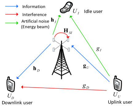
Figure 1: Secrecy SWIPT in full duplex system with SI.

To avoid the information leakage, artificial noise is utilized at FD-BS to improve the security from physical layer. Denote the transmit signal sent by FD-BS as

$${{\mathbf{x}}_{D}}={{\mathbf{s}}_{D}}+{\mathbf{v}},$$ (1)

where ${{\mathbf{s}}_{D}}\in{\mathbb{C}^{{N_{T}}\times 1}}$ is the transmitted data vector intended for $U_{D}$ which is a complex Gaussian random vector with zero mean and covariance matrix ${\mathbf{S}}\succeq\mathbf{0}$, i.e., ${{\mathbf{s}}_{D}}\sim{\cal CN}(\mathbf{0},{\mathbf{S}})$. ${\mathbf{v}}\in{\mathbb{C}^{{N_{T}}\times 1}}$ is the artificial noise vector generated by the FD-BS to combat the curious or even adversarial idle user. Similarly, ${\mathbf{v}}\sim{\cal CN}(\mathbf{0},{\mathbf{V}})$, ${\mathbf{V}}\succeq\mathbf{0}$ . Since the idle user harvests energy from the FD-BS, the artificial noise vector also plays the role of energy vector.

Suppose ${s_{U}}\sim{\cal CN}(0,1)$ is the data symbol transmitted by uplink user and denote $P_{U}$ as its corresponding transmission power. Then, the information transmitted by uplink user is given as ${x_{U}}=\sqrt{{P_{U}}}{s_{U}}$.

The signal received by downlink user $U_{D}$ and idle user $U_{I}$ are respectively given by

$${y_{D}}={\mathbf{h}}_{D}^{H}{{\mathbf{s}}_{D}}+{\mathbf{h}}_{D}^{H}{\mathbf{v}}+{g_{D}}{x_{U}}+{z_{D}}$$ (2)

$$\!\!\!\!\!\!\!\!\!\!\!\!\!\!\text{and}~{}~{}{y_{I}}={\mathbf{h}}_{I}^{H}{{\mathbf{s}}_{D}}+{\mathbf{h}}_{I}^{H}{\mathbf{v}}+{g_{I}}{x_{U}}+{z_{I}},$$ (3)

where ${{\mathbf{h}}_{D}}\in{\mathbb{C}^{{N_{T}}\times 1}}$ and ${{\mathbf{h}}_{I}}\in{\mathbb{C}^{{N_{T}}\times 1}}$ denote the channel vector from FD-BS to user $U_{D}$ and $U_{I}$, respectively. $g_{I}$ and $g_{D}$ represent the complex channel coefficient from $U_{U}$ to $U_{I}$ and $U_{D}$, respectively. ${z_{D}},{z_{I}}\sim{\cal CN}(0,\sigma_{Z}^{2})$ are the corresponding background noise at $U_{D}$ and $U_{I}$, respectively.

After the receiver vector ${{\mathbf{w}}_{R}}$, the received signal at FD-BS is given as

$${y_{U}}={\mathbf{w}}_{R}^{H}{{\mathbf{g}}_{U}}\sqrt{{P_{U}}}{s_{U}}+{{\mathbf{w}}_{R}^{H}{{\mathbf{H}}_{SI}}({{\mathbf{s}}_{D}}+{\mathbf{v}})}+{\mathbf{w}}_{R}^{H}{{\mathbf{z}}_{U}},$$ (4)

where ${{\mathbf{g}}_{U}}\in{\mathbb{C}^{{N_{R}}\times 1}}$ is the complex channel vector from the FD-BS to uplink user $U_{U}$ and ${\mathbf{z}_{U}}\sim{\cal CN}(\mathbf{0},\sigma_{Z}^{2}{{\mathbf{I}}_{{N_{R}}}})$ is the noise vector received at the FD-BS. ${{\mathbf{H}}_{SI}}\in{\mathbb{C}^{{N_{R}}\times{N_{T}}}}$ is the residual SI channel from transmit antennas to the receive antennas at FD-BS.

From (2) and (4), the received signal to interference plus noise ratio (SINR) at downlink user $U_{D}$ and FD-BS can be respectively expressed as

$${\gamma_{D}}=\frac{{{\mathbf{h}}_{D}^{H}{\mathbf{S}}{{\mathbf{h}}_{D}}}}{{{\mathbf{h}}_{D}^{H}{\mathbf{V}}{{\mathbf{h}}_{D}}+{P_{U}}{{\left|{{g_{D}}}\right|}^{2}}+\sigma_{Z}^{2}}}$$ (5)

$$\text{and}~{}~{}{\gamma_{U}}=\frac{{{P_{U}}{{\left|{{\mathbf{w}}_{R}^{H}{{\mathbf{g}}_{U}}}\right|}^{2}}}}{{{\mathbf{w}}_{R}^{H}{{\mathbf{H}}_{SI}}{\mathbf{(S+V)H}}_{SI}^{H}{{\mathbf{w}}_{R}}+\sigma_{z}^{2}\left\|{{\mathbf{w}}_{R}}\right\|_{2}^{2}}}.$$ (6)

The idle user is assumed to process the downlink and uplink signals independently [7]. Thereby, from (3), the corresponding SINR of the downlink and uplink signals at idle user are respectively given as

$${\gamma_{I}^{D}}=\frac{{{\mathbf{h}}_{I}^{H}{\mathbf{S}}{{\mathbf{h}}_{I}}}}{{{\mathbf{h}}_{I}^{H}{\mathbf{V}}{{\mathbf{h}}_{I}}+{P_{U}}{{\left|{{g_{I}}}\right|}^{2}}+\sigma_{Z}^{2}}}$$ (7)

$$\text{and}~{}~{}{\gamma_{I}^{U}}=\frac{{P_{U}}{{\left|{{g_{I}}}\right|}^{2}}}{{{\mathbf{h}}_{I}^{H}{\mathbf{V}}{{\mathbf{h}}_{I}}+{\mathbf{h}}_{I}^{H}{\mathbf{S}}{{\mathbf{h}}_{I}}+\sigma_{Z}^{2}}}.$$ (8)

Different from the HD-BS, both downlink and uplink security can be concurrently guaranteed by the AN sent by FD-BS.

The achievable secrecy rates of downlink and uplink channel can be respectively expressed as

$$R_{D}^{\sec}({\mathbf{S}},{\mathbf{V}}) =\Big{[}{\log_{2}}(1+{\gamma_{D}})-{\log_{2}}(1+{\gamma_{I}^{D}})\Big{]}^{+}~{}~{}\text{and}$$ (9)

$${R_{U}^{sec}}({\mathbf{S}},{\mathbf{V}},{{\mathbf{w}}_{R}})=\Big{[}{\log_{2}}\left({1+{\gamma_{U}}}\right)-{\log_{2}}\left({1+{\gamma_{I}^{U}}}\right)\Big{]}^{+},$$ (10)

where $[x]^{+}\triangleq\max\{0,x\}$.

On the other hand, the harvested energy at $U_{I}$ is given by

$$E=\zeta\left({{\mathbf{h}}_{I}^{H}{\mathbf{S}}{{\mathbf{h}}_{I}}+{\mathbf{h}}_{I}^{H}{\mathbf{V}}{{\mathbf{h}}_{I}}+{P_{U}}{{\left|{{g_{I}}}\right|}^{2}}}\right),$$ (11)

where $0<\zeta\leqslant 1$ is a constant, denoting the RF energy conversion efficiency of the idle user.

In this letter, we focus on the joint design of transceiver information covariance matrix, AN covariance matrix and receiver vector to maximize the total secure downlink and uplink transmission rate under the sum transmission power constraint at FD-BS and the harvested energy constraint at idle user. Specifically, the problem is formulated as

$$\mathcal{P}1: ~{}~{}~{}~{}\underset{{{\mathbf{S}},{\mathbf{V}},{{\left\|{{{\mathbf{w}}_{R}}}\right\|}_{2}^{2}}=1}}{\text{max}} \!\!\!\!\!\!\!\!\!\!\!\!\!\!\!\!\!\!\!\!\!\!\!\!\!\!\!R_{D}^{\sec}({\mathbf{S}},{\mathbf{V}})+{R_{U}^{sec}}({\mathbf{S}},{\mathbf{V}},{{\mathbf{w}}_{R}})$$ (12a)

s. t. $$\!\!\!\!\!\!\!\!\!\!\!\!\!\!\!\!\!\!\!\!\!\!\!\!\!\!\!\operatorname{Tr}({\mathbf{S}})+\operatorname{Tr}({\mathbf{V}})\leqslant{P_{BS}},$$ (12b)

$$\!\!\!\!\!\!\!\!\!\!\!\!\!\!\!\!\!\!\!\!\!\!\!\!\!\!\!\!\!\!\!\!\!\!\!\!\!\!\!\zeta\left({{\mathbf{h}}_{I}^{H}{\mathbf{S}}{{\mathbf{h}}_{I}}+{\mathbf{h}}_{I}^{H}{\mathbf{V}}{{\mathbf{h}}_{I}}+{P_{U}}{{\left|{{g_{I}}}\right|}^{2}}}\right)\geqslant{E_{min}},$$ (12c)

where $P_{BS}$ is the maximum power at the FD-BS and $E_{min}$ is the minimum requirement of the harvested energy at $U_{I}$.

Notice that the feasible condition of problem $\mathcal{P}$1 is that ${E_{min}}\leqslant\zeta\left({{P_{BS}}\left\|{{{\mathbf{h}}_{I}}}\right\|_{2}^{2}+{P_{U}}{{\left|{{g_{I}}}\right|}^{2}}}\right)$ [11]. Throughout this letter, we consider the non-trivial case where the optimization problem is feasible. Obviously, problem $\mathcal{P}$1 is a non-convex problem. Therefore, the key idea to solve problem $\mathcal{P}$1 is the reformulation of the objective function.

III Optimization for The Sum of Downlink and Uplink Secrecy Rate

Observe that constraints (12b) and (12c) depend on variables $\mathbf{S}$ and $\mathbf{V}$, while constraint ${{\left\|{{{\mathbf{w}}_{R}}}\right\|}_{2}^{2}}=1$ depends on variable $\mathbf{w}_{R}$. That is, constraints (12b) and (12c) are independent with ${{\left\|{{{\mathbf{w}}_{R}}}\right\|}_{2}^{2}}=1$. So we can solve problem $\mathcal{P}$1 by first maximizing over ${{\mathbf{w}}_{R}}$, and then maximizing over $\mathbf{S}$ and $\mathbf{V}$ [12].

Given the fixed $\mathbf{S}$ and $\mathbf{V}$, the optimization of problem $\mathcal{P}1$ is equivalent to maximize the uplink rate by finding the optimal receiver vector ${{\mathbf{w}}_{R}}$. Considering that the uplink channel is a SIMO channel, the optimal unit receiver vector to maximize the SINR $\gamma_{U}$ is expressed as [13]

$${{\mathbf{w}}_{R}}=\frac{{{{\left({\sigma_{Z}^{2}{{\mathbf{I}}_{{N_{R}}}}+{{\mathbf{H}}_{SI}}({\mathbf{S}}+{\mathbf{V}}){\mathbf{H}}_{SI}^{H}}\right)}^{-1}}{{\mathbf{g}}_{U}}}}{{\left\|{{{\left({\sigma_{Z}^{2}{{\mathbf{I}}_{{N_{R}}}}+{{\mathbf{H}}_{SI}}({\mathbf{S}}+{\mathbf{V}}){\mathbf{H}}_{SI}^{H}}\right)}^{-1}}{{\mathbf{g}}_{U}}}\right\|}_{2}}.$$ (13)

Then, the uplink SINR at FD-BS is rewritten as

$$\begin{split}{\gamma_{U}}={P_{U}}{\mathbf{g}}_{U}^{H}{{\left({\sigma_{Z}^{2}{{\mathbf{I}}_{{N_{R}}}}+{{\mathbf{H}}_{SI}}({\mathbf{S}}+{\mathbf{V}}){\mathbf{H}}_{SI}^{H}}\right)}^{-1}}{{\mathbf{g}}_{U}}.\end{split}$$ (14)

Substituting (14) into (10), ${R_{U}^{sec}}({\mathbf{S}},{\mathbf{V}},{{\mathbf{w}}_{R}})$ is consequently changed as ${R_{U}^{sec}}({\mathbf{S}},{\mathbf{V}})$. Then, the problem $\mathcal{P}$1 can be further formulated as follows.

$$\mathcal{P}2:~{}~{}~{}~{}~{} \underset{{{\mathbf{S}},{\mathbf{V}}}}{\text{max}} \!\!\!\!\!\!\!\!\!\!\!\!\!\!\!\!\!\!\!\!\!\!\!\!\!\!\!\!\!\!R_{D}^{\sec}({\mathbf{S}},{\mathbf{V}})+{R_{U}^{sec}}({\mathbf{S}},{\mathbf{V}})$$ (15a)

s. t. $$\!\!\!\!\!\!\!\!\!\!\!\!\!\!\!\!\!\!\!\!\!\!\!\!\!\operatorname{Tr}({\mathbf{S}})+\operatorname{Tr}({\mathbf{V}})\leqslant{P_{BS}},$$ (15b)

$$\!\!\!\!\!\!\!\!\!\!\!\!\!\!\!\!\!\!\!\!\!\!\!\!\!\!\!\!\!\!\!\!\!\!\!\zeta\left({{\mathbf{h}}_{I}^{H}{\mathbf{S}}{{\mathbf{h}}_{I}}+{\mathbf{h}}_{I}^{H}{\mathbf{V}}{{\mathbf{h}}_{I}}+{P_{U}}{{\left|{{g_{I}}}\right|}^{2}}}\right)\geqslant{E_{min}}.$$ (15c)

Although we have fixed the receiver vector, the objective function of problem $\mathcal{P}$2 is still complicated and non-convex. It is of importance to transform this problem into a tractable form. Motivated by the log-exponential reformulation idea in [14], we introduce slack variables $\{{x_{D}},{y_{D}},{x_{I}},{y_{I}},{t_{U}},{y_{U}}\}$ to rewrite the problem $\mathcal{P}$2 as the following $\mathcal{P}$2.1:

$$\underset{{{\mathbf{S}},{\mathbf{V}},{x_{D}},{y_{D}},\atop{x_{I}},{y_{I}},{t_{U}},{y_{U}}}}{\text{max}} \!\!\!\!\!\!\!\!\!\!\!\!\!\!\!\!\!\!\!({x_{D}}-{y_{D}}-{x_{I}}+{y_{I}}+{t_{U}}-{x_{I}}+{y_{U}}){\log_{2}}e$$ (16a)

s. t. $$\!\!\!\!\!\!\!\!\!\!\!\!{\mathbf{h}}_{D}^{H}{\mathbf{S}}{{\mathbf{h}}_{D}}+{\mathbf{h}}_{D}^{H}{\mathbf{V}}{{\mathbf{h}}_{D}}+{P_{U}}{{\left|{{g_{D}}}\right|}^{2}}+\sigma_{Z}^{2}\geqslant{e^{{x_{D}}}},$$ (16b)

$$\!\!\!\!\!\!\!\!\!\!\!\!{\mathbf{h}}_{D}^{H}{\mathbf{V}}{{\mathbf{h}}_{D}}+{P_{U}}{{\left|{{g_{D}}}\right|}^{2}}+\sigma_{Z}^{2}\leqslant{e^{{y_{D}}}},$$ (16c)

$$\!\!\!\!\!\!\!\!\!\!\!\!{\mathbf{h}}_{I}^{H}{\mathbf{S}}{{\mathbf{h}}_{I}}+{\mathbf{h}}_{I}^{H}{\mathbf{V}}{{\mathbf{h}}_{I}}+{P_{U}}{\left|{{g_{I}}}\right|^{2}}+\sigma_{Z}^{2}\leqslant{e^{{x_{I}}}},$$ (16d)

$$\!\!\!\!\!\!\!\!\!\!\!\!{\mathbf{h}}_{I}^{H}{\mathbf{V}}{{\mathbf{h}}_{I}}+{P_{U}}{\left|{{g_{I}}}\right|^{2}}+\sigma_{Z}^{2}\geqslant{e^{{y_{I}}}},$$ (16e)

$$\!\!\!\!\!\!\!\!\!\!\!\!({x_{D}}-{y_{D}}-{x_{I}}+{y_{I}}){\log_{2}}e\geqslant 0,$$ (16f)

$$\!\!\!\!\!\!\!\!\!\!\!\!{P_{U}}{\mathbf{g}}_{U}^{H}{\left({\sigma_{Z}^{2}{{\mathbf{I}}_{{N_{R}}}}+{{\mathbf{H}}_{SI}}({\mathbf{S}}+{\mathbf{V}}){\mathbf{H}}_{SI}^{H}}\right)^{-1}}{{\mathbf{g}}_{U}}\geqslant{e^{{t_{U}}}}-1,$$ (16g)

$$\!\!\!\!\!\!\!\!\!\!\!\!{\mathbf{h}}_{I}^{H}{\mathbf{S}}{{\mathbf{h}}_{I}}+{\mathbf{h}}_{I}^{H}{\mathbf{V}}{{\mathbf{h}}_{I}}+\sigma_{Z}^{2}\geqslant{e^{{y_{U}}}},$$ (16h)

$$\!\!\!\!\!\!\!\!\!\!\!\!(t_{U}-x_{I}+y_{U}){\log_{2}}e\geqslant 0,$$ (16i)

$$\!\!\!\!\!\!\!\!\!\!\!\!\operatorname{Tr}({\mathbf{S}})+\operatorname{Tr}({\mathbf{V}})\leqslant{P_{BS}},$$ (16j)

$$\!\!\!\!\!\!\!\!\!\!\!\!\zeta\left({{\mathbf{h}}_{I}^{H}{\mathbf{S}}{{\mathbf{h}}_{I}}+{\mathbf{h}}_{I}^{H}{\mathbf{V}}{{\mathbf{h}}_{I}}+{P_{U}}{{\left|{{g_{I}}}\right|}^{2}}}\right)\geqslant{E_{min}}.$$ (16k)

The objective function (15a) is equivalently decomposed into the objective function (16a) and the eight constraints of (16b)-(16i). In particular, except for (16f) and (16i), the remaining six constraints will hold with equality at the optimum. If (16b) is not active at the optimality point, one can increase $x_{D}$ with a very small value, which improves the objective value while keeping other constraints unchanged. This contradicts the optimality point assumption. Other constraints can be proved in the same way. In addition, the constraints (16f) and (16i) are to guarantee the non-negative secrecy rates of downlink and uplink, respectively. Hence, problem $\mathcal{P}$2.1 is equivalent to $\mathcal{P}$2.

However, the problem $\mathcal{P}$2.1 is still non-convex due to (16c), (16d) and (16g). In order to solve it efficiently, we resort to an iterative algorithm based on sequential parametric convex approximation (SPCA) method [15] to find an approximate solution. The non-convex parts of these constraints are iteratively linearized to its first-order Tayor expansion.

To show this, let us first tackle the non-convex constraints (16c) and (16d). Suppose that, at iteration $n$, ${\mathbf{S}^{*}[n-1]}$, ${\mathbf{V}^{*}[n-1]}$, ${y_{D}^{*}}[n-1]$ and ${x_{I}^{*}}[n-1]$ are given. A concave lower bound of $e^{y_{D}}$ in (16c) can be found as its first order approximation at a neighborhood of ${y_{D}^{*}}[n-1]$ because of the convexity of $e^{y_{D}}$. That is to say,

$${e^{{{y}_{D}^{*}}[n-1]}}({y_{D}}-{y_{D}^{*}}[n-1]+1)\leqslant{e^{{y_{D}}}}$$ (17)

holds, implying that the approximation is conservative for (16c). Similarly, we can replace ${e^{{x_{I}}}}$ by its conservative first order approximation ${{e^{{{x}_{I}^{*}}[n-1]}}({x_{I}}-{x_{I}^{*}}[n-1]+1)}$ in (16d).

Then, we turn our attention to (16g). From [5], we know that ${P_{U}}{\mathbf{g}}_{U}^{H}{\left({\sigma_{Z}^{2}{{\mathbf{I}}_{{N_{R}}}}+{{\mathbf{H}}_{SI}}({\mathbf{S}}+{\mathbf{V}}){\mathbf{H}}_{SI}^{H}}\right)^{-1}}{{\mathbf{g}}_{U}}$ is also joint convex with respect to ${\mathbf{S}}$ and ${\mathbf{V}}$, which is proved by epigraph and Schur complement. For ease of description, let ${{\mathbf{X}}_{U}}=\sigma_{Z}^{2}{{\mathbf{I}}_{{N_{R}}}}+{{\mathbf{H}}_{SI}}({\mathbf{S}}+{\mathbf{V}}){\mathbf{H}}_{SI}^{H}$ and ${{{\mathbf{X^{*}_{U}}}}}[n-1]=\sigma_{Z}^{2}{{\mathbf{I}}_{{N_{R}}}}+{{\mathbf{H}}_{SI}}({\mathbf{S}^{*}[n-1]}+{\mathbf{V}^{*}[n-1]}){\mathbf{H}}_{SI}^{H}$. Further define $G({{\mathbf{X}}_{U}},{{{\mathbf{X^{*}_{U}}}}}[n-1])$ as the first order approximation of ${P_{U}}{\mathbf{g}}_{U}^{H}{{{\mathbf{X}}_{U}}^{-1}}{{\mathbf{g}}_{U}}$. In the same spirit as before, we have

$$\begin{split}&G({{\mathbf{X}}_{U}},{{{\mathbf{X^{*}_{U}}}}}[n-1])={P_{U}}{\mathbf{g}}_{U}^{H}{{{\mathbf{X^{*}_{U}}}}}{[n-1]^{-1}}{{\mathbf{g}}_{U}}\\ &-\operatorname{Tr}\Big{[}\left({{P_{U}}{{{\mathbf{X^{*}_{U}}}}}{{[n-1]}^{-1}}{{\mathbf{g}}_{U}}{\mathbf{g}}_{U}^{H}{{{\mathbf{X^{*}_{U}}}}}{{[n-1]}^{-1}}}\right)\\ &\left({{{\mathbf{X}}_{U}}-{{{\mathbf{X^{*}_{U}}}}}[n-1]}\right)\Big{]}\leqslant{P_{U}}{\mathbf{g}}_{U}^{H}{{\mathbf{X}}_{U}^{-1}}{{\mathbf{g}}_{U}}.\end{split}$$ (18)

To derive (18), we have used the fact that ${\nabla_{\mathbf{A}}}{{\mathbf{a}}^{H}}{{\mathbf{A}}^{-1}}{\mathbf{b}}=-{{\mathbf{A}}^{-1}}{\mathbf{a}}{{\mathbf{b}}^{H}}{{\mathbf{A}}^{-1}}$ for ${\mathbf{A}}\succeq\mathbf{0}$ [16].

Consequently, the convex approximate problem at iteration $n$ is the following problem $\mathcal{P}$2.2 :

$$\underset{{{\mathbf{S}},{\mathbf{V}},{x_{D}},{y_{D}},\atop{x_{I}},{y_{I}},{t_{U}},{y_{U}}}}{\text{max}} \!\!\!\!\!\!\!\!\!({x_{D}}-{y_{D}}-{x_{I}}+{y_{I}}+{t_{U}}-{x_{I}}+{y_{U}}){\log_{2}}e$$ (19a)

s. t. $$\!\!\!\!\!\!\!\!{\mathbf{h}}_{D}^{H}{\mathbf{V}}{{\mathbf{h}}_{D}}+{P_{U}}{{\left|{{g_{D}}}\right|}^{2}}+\sigma_{Z}^{2}\leqslant{e^{{{y}^{*}_{D}}[n-1]}}({y_{D}}-{{y}^{*}_{D}}[n-1]+1),$$ (19b)

$$\!\!\!\!\!\!\!\!\!\!\!\!\!\!\!\!{\mathbf{h}}_{I}^{H}{\mathbf{S}}{{\mathbf{h}}_{I}}+{\mathbf{h}}_{I}^{H}{\mathbf{V}}{{\mathbf{h}}_{I}}+{P_{U}}{\left|{{g_{I}}}\right|^{2}}+\sigma_{Z}^{2}\leqslant{e^{{{x}^{*}_{I}}[n-1]}}({x_{I}}-{{x}^{*}_{I}}[n-1]+1),$$ (19c)

$$\!\!\!\!\!\!\!\!\!\!\!\!\!\!\!\!G({{\mathbf{X}}_{U}},{{{\mathbf{X}}}^{*}_{U}}[n-1])\geqslant{e^{{t_{U}}}}-1,$$ (19d)

$$\!\!\!\!\!\!\!\!\!\!\!\!\!\!\!\!\text{(16b), (16e), (16f), (16h)-(16k)}.\$$ (19e)

This is a convex SDP which can be solved efficiently by off-the-shelf solvers, e.g., CVX [17]. By solving this problem, we can obtain ${\mathbf{S}^{*}[n]}$, ${\mathbf{V}^{*}[n]}$, ${y_{D}^{*}}[n]$, ${x_{I}^{*}}[n]$ as well as the achieved sum secrecy rate $u[n]$. Detailed steps to solve problem $\mathcal{P}$2 are stated in Algorithm 1. According to [15], Algorithm 1 converges to a KKT point of problem $\mathcal{P}2$. Detailed proof is presented in Appendix A. It is worth noting that the iterative procedure in Algorithm 1 may return a locally optimal solution to problem $\mathcal{P}$2.

Algorithm 1 SPCA method for problem $\mathcal{P}$2

1:  Initialize feasible points for ${\mathbf{S}^{*}[0]}$ and ${\mathbf{V}^{*}[0]}$ by solving the feasibility problem of $\mathcal{P}$2 (replace (15a) with 0);

2:  Calculate ${{y}^{*}_{D}}[0]=\ln({\mathbf{h}}_{D}^{H}{\mathbf{V}^{*}[0]}{{\mathbf{h}}_{D}}+{P_{U}}{{\left|{{g_{D}}}\right|}^{2}}+\sigma_{Z}^{2})$ and ${{x}^{*}_{I}}[0]=\ln({\mathbf{h}}_{I}^{H}{\mathbf{S}^{*}[0]}{{\mathbf{h}}_{I}}+{\mathbf{h}}_{I}^{H}{\mathbf{V}^{*}[0]}{{\mathbf{h}}_{I}}+{P_{U}}{\left|{{g_{I}}}\right|^{2}}+\sigma_{Z}^{2})$;

3:  Set $n:=0$;

4:  while $\frac{{u[n]-u[n-1]}}{{u[n-1]}}\geqslant{10^{-3}}$ do

5:     Solve problem $\mathcal{P}$2.2 by CVX to obtain ${\mathbf{S}^{*}[n]}$, ${\mathbf{V}^{*}[n]}$, ${y_{D}^{*}}[n]$ and ${x_{I}^{*}}[n]$;

6:     Set $n:=n+1$;

7:  end while

8:  return  ${\mathbf{S}^{*}[n]}$ and ${\mathbf{V}^{*}[n]}$ as an approximate solution.

IV Simulation Results

In this section, simulation results are presented to evaluate the performance of our proposed schemes. We assume that FD-BS is equipped with $N_{T}=4$ and $N_{R}=4$ antennas and its transmission power is ${P_{BS}}=1$ W. The uplink user transmission power is 0.1 W. For simplicity, we set the energy harvesting efficiency as 50$\%$. All the receiver noise power equals to $-80$ dB. Assume that the signal attenuation from FD-BS to idle user is 30 dB and the remaining channel attenuations are 70 dB excluding the residual SI channel. These channel entries are independently generated from i.i.d Rayleigh fading with the respective average power values. Besides, we generate the elements of ${{\mathbf{H}}_{SI}}$ as ${\cal CN}(0,\sigma_{SI}^{2})$, where $\sigma_{SI}^{2}$ depends on the capability of the SIC techniques. For comparison, we also introduce two schemes, i.e., perfect full duplex and two-phase half duplex. In the half duplex scheme, all $N=8$ antennas are used for data transmission/reception in 1/2 time slot.

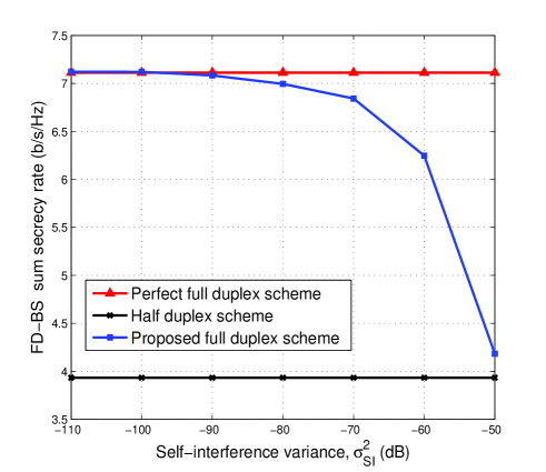
Figure 2: Achievable sum secrecy rate versus self-interference variance for different schemes with $E_{min}=1$ mW.

In Fig. 2, the impact of self-interference variance on the achievable sum secrecy rate is presented with $E_{min}=1$ mW. As expected, we can see that the performance of our proposed full duplex scheme degrades as $\sigma_{SI}^{2}$ increases, while that of other schemes remain the same.

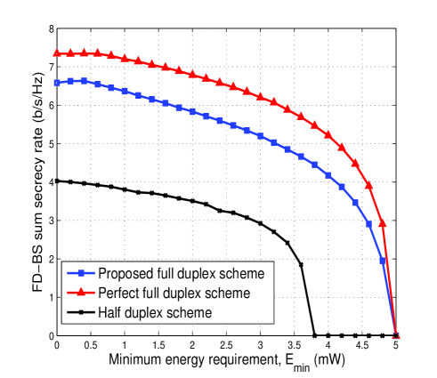
Figure 3: Achievable sum secrecy rate versus minimum energy requirement for different schemes with $\sigma_{SI}^{2}=-60$ dB.

Fig. 3 compares the sum secrecy rate of different schemes versus minimum energy requirement with $\sigma_{SI}^{2}=-60$ dB. According to Fig. 3, it is straightforward that the secrecy sum rate decreases as the minimum energy requirement increases. Besides, the performance of our proposed full duplex scheme extremely outperforms that of half duplex scheme by 65%, which greatly verifies the superiority of our proposed system.

V Conclusion

This letter has designed a transceiver scheme for secure SWIPT in a full duplex wireless system with one downlink user, one uplink user and one idle user. We have jointly optimized the transmitter covariance matrix and receiver vector to maximize the sum of downlink and uplink secrecy rate subject to the sum transmission power constraint at FD-BS and the harvested energy requirement at the idle user. It has been demonstrated that the proposed full duplex scheme yields a large gain than half duplex scheme in terms of the sum secrecy rate.

Appendix A Proof of the convergence for Algorithm 1

In this appendix, we first prove the convergence of Algorithm 1 by adopting the technique from [15]. Let ${\mathcal{S}}^{(n)}$ be the convex set of problem $\mathcal{P}$2.2 at iteration $n$. For ease of presentation, we define

$$\varphi({y_{D}},{\mathbf{V}})={\mathbf{h}}_{D}^{H}{\mathbf{V}}{{\mathbf{h}}_{D}}+{P_{U}}{{\left|{{g_{D}}}\right|}^{2}}+\sigma_{Z}^{2}-{e^{{y_{D}}}}~{}~{}\text{and}$$ (20)

$$\begin{split}&\phi({y_{D}},y_{D}^{*}[n-1],{\mathbf{V}})={\mathbf{h}}_{D}^{H}{\mathbf{V}}{{\mathbf{h}}_{D}}+{P_{U}}{{\left|{{g_{D}}}\right|}^{2}}+\sigma_{Z}^{2}\\ &~{}~{}~{}~{}~{}~{}~{}-{e^{y_{D}^{*}[n-1]}}({y_{D}}-y_{D}^{*}[n-1]+1).\end{split}$$ (21)

Due to (17) and (19b), we have

$$\varphi({y_{D}},{\mathbf{V}})\leqslant\phi({y_{D}},y_{D}^{*}[n-1],{\mathbf{V}})\leqslant 0.$$ (22)

Since the affine approximation in (17), the following two properties are satisfied.

$${{\phi({y_{D}},y_{D}^{*}[n-1],{\mathbf{V}})}\bigg{|}_{{y_{D}}=y_{D}^{*}[n-1],{\mathbf{V}}={{\mathbf{V}}^{*}}[n-1]}}$$

$$\!\!\!\!\!\!\!={{\varphi({y_{D}},{\mathbf{V}})}\bigg{|}_{{y_{D}}=y_{D}^{*}[n-1],{\mathbf{V}}={{\mathbf{V}}^{*}}[n-1]}}\leqslant 0,$$ (23)

$${{\nabla\phi({y_{D}},y_{D}^{*}[n-1],{\mathbf{V}})}\bigg{|}_{{y_{D}}=y_{D}^{*}[n-1],{\mathbf{V}}={{\mathbf{V}}^{*}}[n-1]}}$$

$$\!\!\!\!\!\!\!\!={{\nabla\varphi({y_{D}},{\mathbf{V}})}\bigg{|}_{{y_{D}}=y_{D}^{*}[n-1],{\mathbf{V}}={{\mathbf{V}}^{*}}[n-1]}}.$$ (24)

From (23), we know that the optimal variables $y_{D}^{*}[n-1]$ and $\mathbf{V}^{*}[n-1]$ obtained at iteration $n-1$ is a feasible solution to the problem $\mathcal{P}$2.2 at iteration $n$. Similarly, the constraints in (19c) and (19d) also have the same properties. In other words, $\left(y_{D}^{*}[n-1],x_{I}^{*}[n-1],\mathbf{S}^{*}[n-1],\mathbf{V}^{*}[n-1]\right)\in\mathcal{S}^{(n)}$ and thus $u[n]\geqslant u[n-1]$. In fact, we have shown that the sequence ${u[n]}$ in nondecreasing. Besides, the value of ${u[n]}$ is bounded above due to the limited transmission power, and thus it is guaranteed to convergence.

Then, similar with that (19b) has two properties, i.e., (23) and (24), (19c) and (19d) also have their corresponding properties, respectively. According to [15, Proposition 3.2], all accumulation points of $\left(y_{D}^{*}[n],x_{I}^{*}[n],\mathbf{S}^{*}[n],\mathbf{V}^{*}[n]\right)$ are KKT points of the original problem $\mathcal{P}$2.1 or $\mathcal{P}$2. Thus, our proposed algorithm 1 converges to a KKT point of problem $\mathcal{P}$2.

References

• [1] D.ย Bharadia, E.ย McMilin, and S.ย Katti, โ€œFull duplex radios,โ€ in Proc. ACM SIGCOMM Computer Communication Review, 2013, pp. 375โ€“386.
• [2] E.ย Ahmed, A.ย M. Eltawil, and A.ย Sabharwal, โ€œSelf-interference cancellation with phase noise induced ici suppression for full-duplex systems,โ€ in Proc. IEEE Global Communications Conference (GLOBECOM), 2013, pp. 3384โ€“3388.
• [3] Y.ย Zeng and R.ย Zhang, โ€œFull-duplex wireless-powered relay with self-energy recycling,โ€ IEEE Wireless Communications Letters, vol.ย 4, no.ย 2, pp. 201โ€“204, Apr. 2015.
• [4] G.ย Zheng, I.ย Krikidis, J.ย Li, A.ย P. Petropulu, and B.ย Ottersten, โ€œImproving physical layer secrecy using full-duplex jamming receivers,โ€ IEEE Transactions on Signal Processing, vol.ย 61, no.ย 20, pp. 4962โ€“4974, Oct. 2013.
• [5] D.ย Nguyen, L.-N. Tran, P.ย Pirinen, and M.ย Latva-Aho, โ€œOn the spectral efficiency of full-duplex small cell wireless systems,โ€ IEEE Transactions on Wireless Communications, vol.ย 13, no.ย 9, pp. 4896โ€“4910, Sept. 2014.
• [6] G.ย Zheng, I.ย Krikidis, and B.ย Ottersten, โ€œFull-duplex cooperative cognitive radio with transmit imperfections,โ€ IEEE Transactions on Wireless Communications, vol.ย 12, no.ย 5, pp. 2498โ€“2511, May 2013.
• [7] F.ย Zhu, F.ย Gao, M.ย Yao, and H.ย Zou, โ€œJoint information-and jamming-beamforming for physical layer security with full duplex base station,โ€ IEEE Transactions on Signal Processing, vol.ย 62, no.ย 24, pp. 6391โ€“6401, Dec. 2014.
• [8] L.ย Liu, R.ย Zhang, and K.-C. Chua, โ€œSecrecy wireless information and power transfer with MISO beamforming,โ€ IEEE Transactions on Signal Processing, vol.ย 62, no.ย 7, pp. 1850โ€“1863, Apr. 2014.
• [9] D.ย W.ย K. Ng and R.ย Schober, โ€œResource allocation for secure communication in systems with wireless information and power transfer,โ€ in Proc. IEEE Globecom Workshops (GC Workshops), 2013, pp. 1251โ€“1257.
• [10] D.ย W.ย K. Ng, L.ย Xiang, and R.ย Schober, โ€œMulti-objective beamforming for secure communication in systems with wireless information and power transfer,โ€ in Proc. IEEE Personal Indoor and Mobile Radio Communications (PIMRC), 2013, pp. 7โ€“12.
• [11] R.ย Zhang and C.ย K. Ho, โ€œMIMO broadcasting for simultaneous wireless information and power transfer,โ€ IEEE Transactions on Wireless Communications, vol.ย 12, no.ย 5, pp. 1989โ€“2001, May 2013.
• [12] S.ย Boyd and L.ย Vandenberghe, Convex optimization.ย ย ย Cambridge University Press, 2004.
• [13] D.ย Tse and P.ย Viswanath, Fundamentals of wireless communication.ย ย ย Cambridge University Press, 2005.
• [14] W.-C. Li, T.-H. Chang, C.ย Lin, and C.-Y. Chi, โ€œCoordinated beamforming for multiuser miso interference channel under rate outage constraints,โ€ IEEE Transactions on Signal Processing, vol.ย 61, no.ย 5, pp. 1087โ€“1103, Mar. 2013.
• [15] A.ย Beck, A.ย Ben-Tal, and L.ย Tetruashvili, โ€œA sequential parametric convex approximation method with applications to nonconvex truss topology design problems,โ€ Journal of Global Optimization, vol.ย 47, no.ย 1, pp. 29โ€“51, Oct. 2010.
• [16] J.ย Dattorro, Convex optimization and Euclidean distance geometry.ย ย ย Meboo Publishing USA, 2010.
• [17] M.ย Grant and S.ย Boyd, โ€œ cvx: Matlab software for disciplined convex programming, version 1.22,โ€ http://cvxr.com/cvx, Aug. 2012.