Sodium Absorption Systems toward SN Ia 2014J Originate on Interstellar Scales²⁰

Abstract

Na I D absorbing systems toward Type Ia supernovae (SNe Ia) have been intensively studied over the last decade with the aim of finding circumstellar material (CSM), which is an indirect probe of the progenitor system. However, it is difficult to deconvolve CSM components from non-variable, and often dominant, components created by interstellar material (ISM). We present a series of high-resolution spectra of SN Ia 2014J from before maximum brightness to $\mathrel{\hbox to0.0pt{\lower 4.0pt\hbox{\hskip 1.0pt$\sim$}\hss}\raise 1.0pt\hbox{$>$}}$250 days after maximum brightness. The late-time spectrum provides unique information for determining the origin of the Na I D absorption systems. The deep late-time observation allows us to probe the environment around the SN at a large scale, extending to $\mathrel{\hbox to0.0pt{\lower 4.0pt\hbox{\hskip 1.0pt$\sim$}\hss}\raise 1.0pt\hbox{$>$}}$40 pc. We find that a spectrum of diffuse light in the vicinity, but not directly in the line-of-sight, of the SN has absorbing systems nearly identical to those obtained for the ‘pure’ SN line-of-sight. Therefore, basically all Na I D systems seen toward SN 2014J must originate from foreground material that extends to at least $\sim$40 pc in projection and none at the CSM scale. A fluctuation in the column densities at a scale of $\sim$20 pc is also identified. After subtracting the diffuse, “background” spectrum, the late-time SN Na I D profile along the SN line-of-sight is consistent with the profile in the near-maximum brightness spectra. The lack of variability on a $\sim$1 year timescale is consistent with the ISM interpretation for the gas.

1. Introduction

Despite their importance for cosmology as standardizable candles and for astrophysics as an origin of Fe-peak elements, the progenitor system of Type Ia supernovae (SNe Ia) has remained as an unresolved and extensively discussed question for many decades (see, e.g., Hillebrandt & Niemeyer, 2000, for a review). In particular, there have been ongoing efforts to discriminate between the so-called single-degenerate (SD) scenario and the double-degenerate (DD) scenario: in the former an SN Ia is a thermonuclear explosion of a nearly Chandrasekhar-mass white dwarf (WD) formed by the accretion of material from a non-degenerate companion star (e.g., Whelan & Iben, 1973; Nomoto, 1982; Hachisu et al., 1999), while in the latter an SN Ia comes from the merger of two WDs (e.g., Iben & Tutukov, 1984; Webbink, 1984).

There are various observational features proposed so far to diagnose a progenitor system of an individual SN as either SD or DD. These methods include the detection of excess emission in the UV and the blue portion of the optical region in the first few days after a SN Ia explosion. The early excessive emission is suggested to be a signature of the impact between the SN ejecta and a non-degenerate binary companion in the SD scenario (Kasen, 2010; Kutsuna & Shigeyama, 2015). Detections of this behavior have been reported for the peculiar SN 2002es-like iPTF14atg (Cao et al., 2015) and the normal SN Ia 2012cg (Marion et al., 2015b). Among other diagnostics, the environment just around the SN progenitor is key, since the SD scenario predicts a relatively ‘dirty’ environment (i.e., having significant circumstellar material; ‘CSM’) through mass loss from the companion and/or nova eruptions, while the DD scenario is thought to lead to a relatively ‘clean’ environment (i.e., a circumstellar environment similar to or less dense than the interstellar medium; ‘ISM’). This picture is complicated by the possibility that a DD progenitor system may also produce a dense CS environment in some cases (e.g., Shen et al., 2013; Raskin & Kasen, 2013; Tanikawa et al., 2015), but in any case the CSM environment provides strong constraints on and insight into progenitor evolution. There is also another scenario, the core-degenerate (CD) model (Sparks & Stecher 1974), which could produce even more massive CSM than the SD (Soker, 2015). We refer to Maoz et al. (2014) for a review of observational constraints on the progenitor systems of SNe Ia.

Among various methods proposed to probe the environment and existence of CSM, increasing attention has been given to narrow-line absorption systems in the lines-of-sight toward SNe Ia over the last decade. SNe offer a unique opportunity to probe diffuse gas in galaxies beyond the local group. Material along the line of sight is backlit by the SN and is detected as absorption features in (especially high-resolution) spectra (e.g., Rich, 1987; Cox & Patat, 2008). However, distinguishing CSM and ISM components is challenging. The SN produces a strong UV radiation field, which can ionize some atomic species if they are sufficiently close. The ionized atoms will then recombine on a timescale of weeks to months, producing variable absorption on this timescale. Therefore, time-variable absorption features provide strong evidence of CSM (Patat et al., 2007; Simon et al., 2009; Sternberg et al., 2014). However, the lack of variability does not imply a lack of CSM, and it has not been clarified for any individual SNe Ia if there are ‘hidden’ CSM components in the non-variable absorption systems. For a statistical sample of SNe Ia, an imbalance between Na I D systems with “blueshifted” and “redshifted” profiles, with there being more “blueshifted” SNe, is indirect evidence for outflows expected to be associated with CSM (Sternberg et al., 2011; Foley et al., 2012; Maguire et al., 2013). This fact has been used as evidence for a population that evolves through the SD path, highlighting the importance of investigating the existence of hidden CSM components in the non-variable Na I D systems.

SN Ia 2014J in M82 ($d\approx 3.8$ Mpc), discovered by Fossey et al. (2014), is the closest SN Ia in the last few decades and provides a unique opportunity to investigate the progenitor issue. Thanks to its proximity, intensive follow-up observations at various wavelengths have been performed for SN 2014J. Optical and NIR observations show that SN 2014J belongs to a class of normal SNe Ia with layered abundance stratification, but with relatively high velocities of absorption lines (e.g., Goobar et al., 2014; Zheng et al., 2014; Marion et al., 2015a; Vacca et al., 2015), in accordance with a spectral synthesis model (Ashall et al., 2014). At late times, there is no detection of H$\alpha$ emission to deep limits, which has been suggested to be a signature of a non-degenerate companion star (Lundqvist et al., 2015). Mid-IR follow-up shows possible enhancement of stable Ni in the inner part of the ejecta (Telesco et al., 2015), which favors an explosion of a Chandrasekhar-mass WD. SN 2014J also became the first (and so far only) example of an SN Ia for which MeV emissions from radioactive decays of ⁵⁶Co were solidly detected (Churazov et al., 2014); there was also probable detection of ⁵⁶Ni decay emissions, which might favor an explosion of a sub-Chandrasekhar mass WD with a He companion star (Diehl et al., 2014). Pre-explosion Hubble Space Telescope (HST)/Chandra images show no apparent source at the position of the SN, excluding a red-giant companion star (Kelly et al., 2014) and a supersoft X-ray source (Nielsen et al., 2014), which is inconsistent with some variants within the SD model. There are also various observations wthat probe the CSM around SN 2014J: there are non-detections of radio and X-ray emission from SN 2014J, which limits the amount of CSM within $\sim$0.01 pc of the SN progenitor (Pérez-Torres et al., 2014; Margutti et al., 2014). Analyses of the extinction curve toward SN 2014J including UV bands result in mixed interpretations — it has been agreed that the extinction curve toward SN 2014J is characterized by a low value of $R_{V}$, while the extinction law is reported to consist of either a single component (Brown et al., 2015; Amanullah et al., 2015) or multiple-components (Foley et al., 2014; Hoang, 2015). If attributed to a single dust component within the ISM, it requires small grains (Gao et al., 2015; Hoang, 2015), which is also consistent with a non-standard polarization curve toward SN 2014J (Kawabata et al., 2014; Patat et al., 2015). In summary, there are multiple and different indications of the progenitor system of SN 2014J, some favoring the SD but others the DD model. Therefore, adding new and independent information is highly valuable.

SN 2014J was closer than another nearby SN Ia, 2011fe in M101 ($d\approx 6.4$ Mpc) which unlike SN 2014J did not have significant extinction. SN 2014J is thus an ideal target with which one can study the origin of the absorption systems with high-spectral resolution observations. Observations by Goobar et al. (2014) showed a strong and complex structure of the Na I D absorption systems toward SN 2014J, as expected from the red color of the SN itself. Welty et al. (2014) presented spectra showing strong absorption systems not only in Na I D, but also in K I, Ca I, Ca II, CH, CH⁺, CN, and a number of diffuse interstellar bands (DIBs), mainly seen in the wavelength ranges corresponding to the saturated component(s) of the Na I D systems (see also Jack et al., 2015). Foley et al. (2014) reported no variability in Na I D and K I beyond the noise level of their spectra in the period from $-9.6$ days to $+18.4$ days, further confirmed by Ritchey et al. (2015) in their spectra taken between $-5.6$ and $+30.4$ days. Graham et al. (2015) also found no variability in Na I D between $-11$ and $+22$ days, but claimed detection of variability in K I for the most blueshifted components at $-144$ km s^-1 and possibly at $-127$ km s^-1, which correspond to an unsaturated component and a saturated one in the Na I D absorption systems, respectively. If this K I variability is caused by the CSM, it would require a few $M_{\odot}$ at the SN vicinity. This led Soker (2015) to conclude that this is only explained by the CD scenario if the absorption systems indeed originate on the CS scale

Table 1Log of Spectroscopic Observations

MJD	Phase	Telescope	Instrument	Resolution	Wavelength Range (Å)	Exposure (s)	Airmass	S/N per pix
56681.5	-8.9	GAO 1.5m	GAOES	$\sim 37,000$	$4,800-6,700$	$1,800\times 6$	1.5	$\sim 60$
56684.6	-5.8	GAO 1.5m	GAOES	$\sim 37,000$	$4,800-6,700$	$1,800\times 8$	1.2	$\sim 100$
56696.6	+6.2	OAO 1.88m	HIDES	$\sim 50,000$	$5,000-7,500$	$1,800\times 2$	1.3	$\sim 45$
56703.5	+13.1	Subaru 8.2m	HDS	$\sim 50,000$	$3,700-6,400$	$1,800\times 1$	1.6	$\sim 170$
56713.6	+23.2	OAO 1.88m	HIDES	$\sim 50,000$	$5,000-7,500$	$1,500\times 4$	1.2	$\sim 30$
56735.5	+45.1	Subaru 8.2m	HDS	$\sim 50,000$	$3,700-6,400$	$900\times 6$	2.5	$\sim 150$
					$6,400-8,500$	$2,400\times 1$
56748.5	+58.1	GAO 1.5m	GAOES	$\sim 37,000$	$4,800-6,700$	$1,800\times 5$	1.2	$\sim 25$
56755.5	+65.1	GAO 1.5m	GAOES	$\sim 37,000$	$4,800-6,700$	$1,800\times 8$	1.2	$\sim 35$
56945.5	+255.1	Subaru 8.2m	HDS	$\sim 40,000$	$3,700-6,400$	$1,800\times 4$	2.8	$\sim 30$

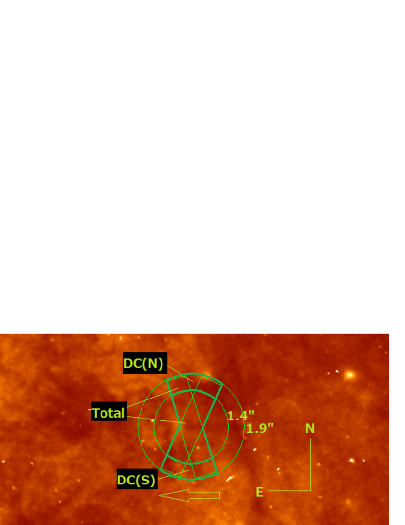
Figure 1.— Pre-explosion image of the position of SN 2014J obtained with HST/ACS/WFC in the F555W filter (Obs Id: 10776, PI: Mountain). The SN position (Crotts, 2015) is at the center of the green circles, which have radii of 1.4 and 1.9″. The slit orientation for the $+255.1$ day spectrum is indicated by the green rectangles – the slit PA was rotated from 197^∘ to 156^∘ during the observation. For our fiducial extraction (‘total’ spectrum), the region along the slit within an aperture of 1.9″(within the outer circle) is integrated. The representative diffuse component spectra are extracted within the region between 1.4″ and 1.9″ (the intersection of the annulus and the rectangles) on both sides of the SN position (N and S), which are further used in extracting a ‘pure’ SN spectrum in the DC model 2.

In this paper, we present a series of high-dispersion spectra of SN 2014J, covering multiple epochs from $-8.9$ to $+255.1$ days relative to $B$-band maximum brightness, collected by three telescopes. Especially unique is our latest spectrum at $+255.1$ days; it is the first high-resolution spectrum taken for any SN Ia at a late-time, nebular phase. This paper focuses on unique information we obtained based on this spectrum, which is qualitatively different from previous analyses performed for high-resolution spectra of SNe. In §2, we summarize observations and our standard data reduction procedures. Results are described in §3. The paper is closed in §4 with conclusions and discussion. Additional analyses are presented in the appendices.

2. Observations and Data Reduction

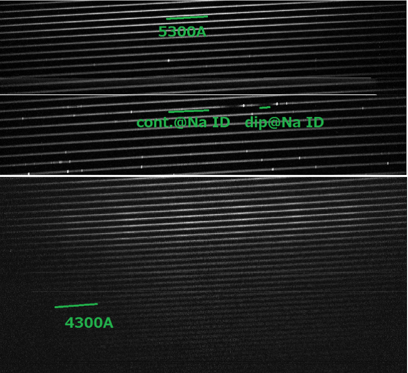
Figure 2.— Two-dimensional spectrum of SN 2014J at $+255.1$ days relative to $B$-band maximum brightness. Spatial profiles (Figure 4) are extracted in the region marked in the figure.

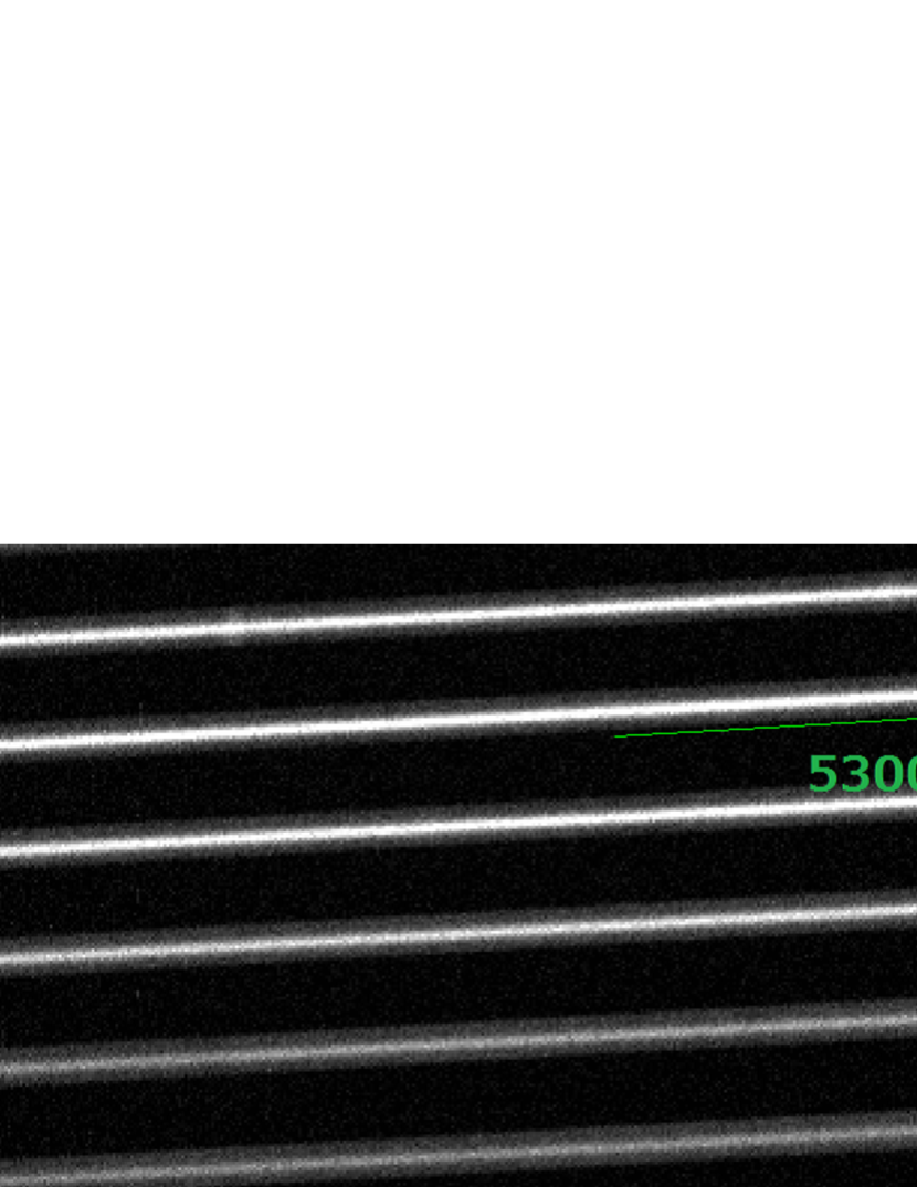
Figure 3.— Expanded view of the two-dimensional spectrum (Figure 2) near $5300$Å, a region where the SN flux is large relative to the background.

A log of our high spectral resolution observations is given in Table 1. We used three telescopes to obtain the spectra, starting at $-8.9$ days relative to $B$-band maximum brightness (MJD 56690.4: Kawabata et al., 2014) and ending at $+255.1$ days: the 1.5-m telescope at the Gunma Astronomical Observatory (GAO) using the GAO Echelle Spectrograph (GAOES), the 1.88-m telescope at the Okayama Astrophysical Observatory (OAO) of National Astronomical Observatory of Japan (NAOJ) with the HIgh Dispersion Echelle Spectrograph (HIDES) in a fiber-feed mode (Kambe et al., 2013), and the 8.2-m Subaru telescope of NAOJ equipped with the High Dispersion Spectrograph (HDS) (Noguchi et al., 2002). The observational parameters (e.g., spectral resolution and wavelength coverage) are shown in Table 1, where the spectral resolution and the signal-to-noise ratio (S/N) at the continuum around Na I D are measured from the reduced spectra.

We followed standard IRAF procedures to reduce the data. Scattered light was subtracted but no further ‘astronomical’ background subtraction was performed in our standard reduction procedure (i.e., generally a typical procedure for high-resolution data reduction). The wavelength calibration was performed using observations of Th-Ar lamps, resulting in an accuracy of $\sim$0.0063 Å for the case of the spectrum at $+255.1$ days. A heliocentric velocity correction was applied to each spectrum, and the wavelength was further redshifted to the M82 rest frame ($z=0.000677$).

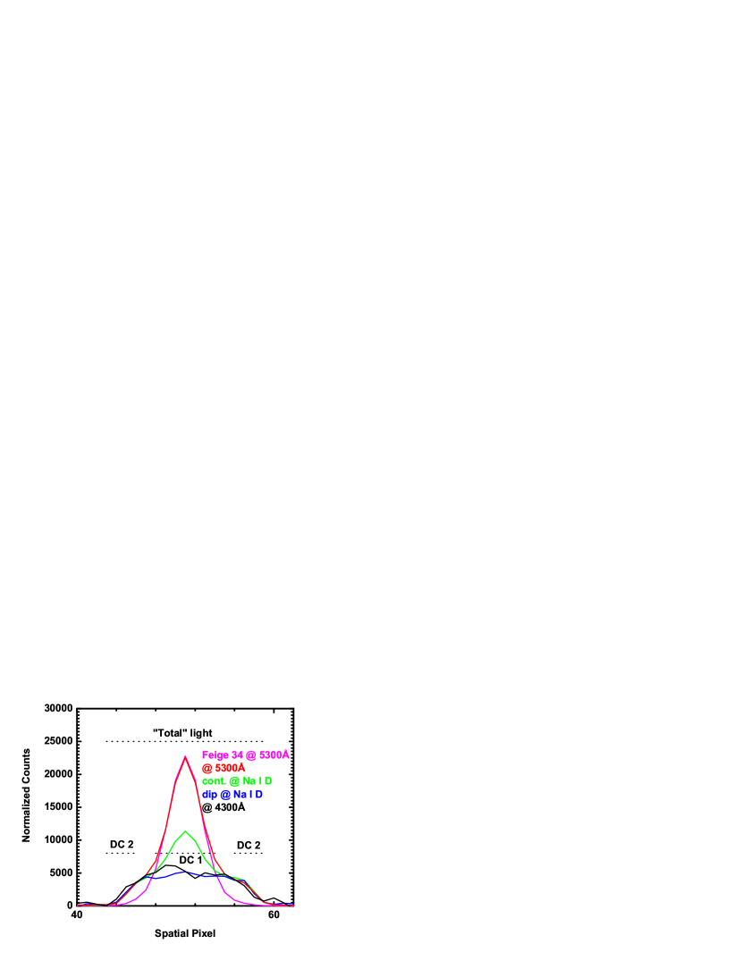
Figure 4.— Spatial profiles of the $+255.1$ day SN 2014J spectrum at different wavelengths: at $\sim$5300 Å where the SN light dominates (red), the region corresponding to the continuum near Na I D where the SN and underlying diffuse light have comparable contributions (green), a region corresponding to strong Na I D absorption (blue) and the continuum at $\sim$4300 Å where the diffuse component dominates over the SN (black). One spatial pixel in this figure has an angular size of $\sim$0.28″ (after the binning before the CCD readout). The fluxes are arbitrarily normalized to provide comparable fluxes in the ‘diffuse’ component at different wavelengths. For comparison, the spatial profile of a spectrum of the standard star Feige 34 is shown for the $\lambda\sim 5300$ Å (magenta).

To produce continuum-normalized flux spectra, first the continuum was fit for each order separately, and the resulting blaze function was then applied to the original spectra when convolving the spectra from different orders. To obtain the continuum-normalized sky spectra, the same procedures were performed for telluric standard stars. The continuum-normalized SN spectra were then divided by the continuum-normalized sky spectra to remove telluric absorption. We did not remove the Milky Way (MW) absorption features in the sky spectra, and this could induce the appearance of variable MW features; however, we do not believe any such variability is real.

Additionally, we created a flux-calibrated version of the $+255.1$ day spectrum. A flux standard star, Feige 34 (Oke, 1990), was observed during the same night with the same settings, and the sensitivity function was derived for each order, which we applied to the SN spectrum. The sky subtraction was not performed for this spectrum, but it does not affect our results derived from the flux-calibrated spectrum.

In this paper, we will mostly focus on implications obtained from the $+255.1$ day spectrum; here we provide a more detailed description of its observation and data reduction. Figure 1 shows our observational setup (slit size and angle) for this observation, overlapped with a pre-explosion image taken by HST/ACS/WCS in the F555W filter (Obs ID: 10776, PI: Mountain, see also Crotts, 2015). For this observation, we did not use an image rotator, but did employ an atmospheric dispersion corrector. The slit position angle (PA) was rotated from 197 deg to 156 deg during the sequence of exposures that total $7,200$ sec. Namely, on average the slit direction was north (N) - south (S), but we collected the light within the region extending to $\pm$20 degree in PA.

Four exposures of $1800$ sec each were obtained for the $+255.1$ day spectrum. The airmass was high, varying from 2.8 to 2.1. In Appendix A, we checked the possibility that the high airmass might introduce any systematic effects, and we conclude that such a possibility is highly unlikely. The 2D spectrum from $+255.1$ days (with the four exposures combined) is shown in Figure 2, and an expanded view around the wavelength region where the SN flux is high ($\sim$5300 Å) is shown in Figure 3. The 2D spectrum shows that the SN is clearly detected. Figure 4 shows the spatial distribution of the incoming light for different wavelength regions (see Figure 2). We see two components, one with a FWHM (full width at half-maximum) of $\sim$0.8″ whose flux strongly depends on the wavelength, and another component extending through the entire aperture whose spatial profile is not sensitive to the wavelength. For comparison, the spectrum of the flux standard star (Feige 34) taken on the same night shows only a single component without an extended component (Figure 4). In the SN spectrum, there is a clear trend that the first component is seen only in the wavelength range where the SN is expected to be bright – for example, at $\sim$4,300 Å the flux is low (Figure 2) and indeed only the second, extended component is identified (Figure 4). We identify the former as the SN contribution and the latter as diffuse light from the region near SN 2014J in M82 (see §3 for further details). In our default spectral extraction, the spectrum was extracted within the whole aperture, which is $0.8\times 3.8$ arcsec² (shown as ‘total’ in Figures 1 and 4). This turns out to be important, and we will revisit this issue in §3.

3. Results

3.1. Variable Na I D Systems at Late Times?

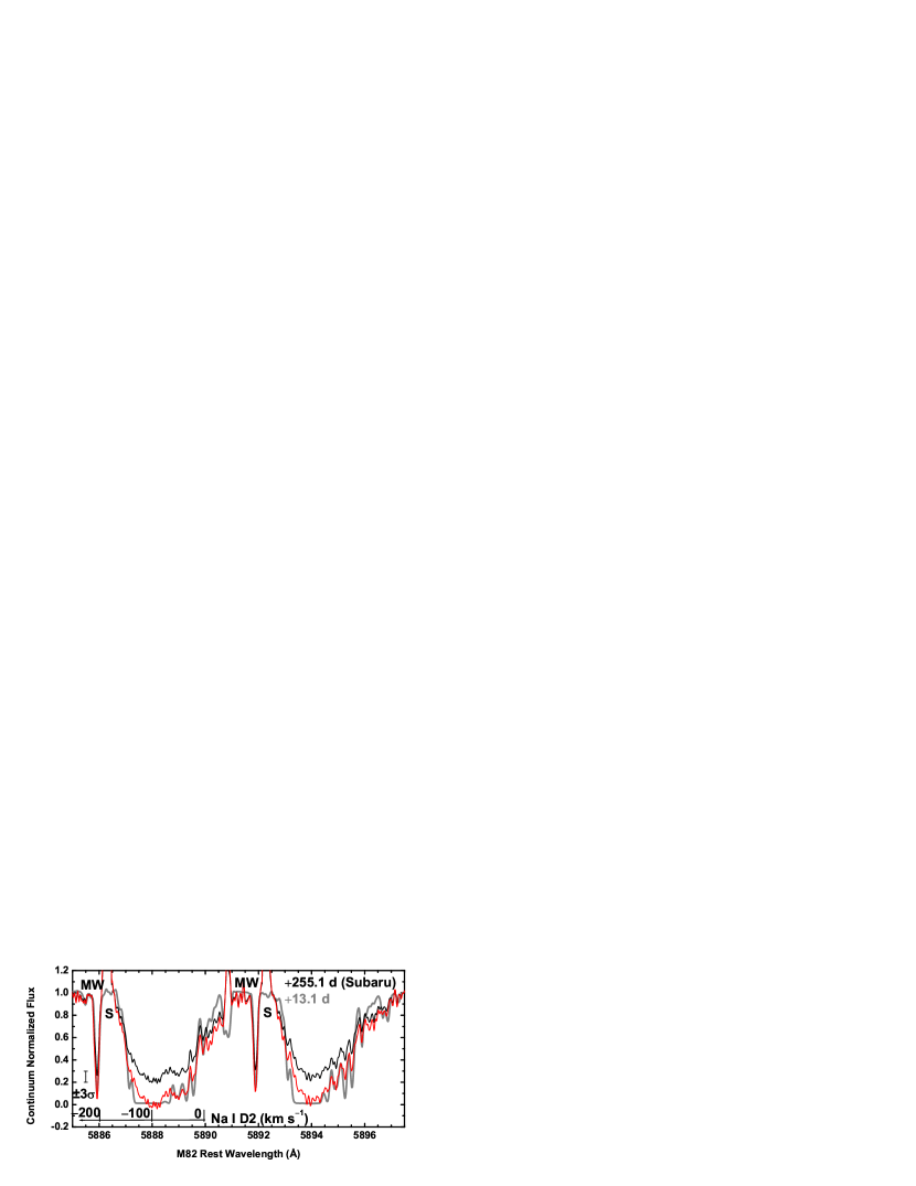
Figure 5.— Series of high-resolution spectra of SN 2014J (black). The spectra are sky-subtracted using telluric standard stars (see §2 for details). In each panel, the spectrum at $+13.1$ days taken by the Subaru telescope is shown for comparison (gray), and is convolved with a Gaussian kernel to provide a comparable spectral resolution for each spectrum. For the $+255.1$ day spectrum, the original spectrum (black) shows an offset in the base of the (previously) saturated components clearly exceeding the noise level. A spectrum after subtracting a constant flux is shown in red. A velocity scale for Na I D2 in the M82 rest frame is indicated in the last panel. The night-sky emissions of Na I D1 and D2 are marked by ‘S’ and the Milky Way components are marked by ‘MW’ in the lower two panels.

Figure 5 shows our high-resolution spectral series of SN 2014J, focusing on the wavelength range covering Na I D1 (5895.92 Å) and D2 (5889.95 Å). The first five spectra ($-8.9$ to $+23.2$ days) confirm the result from the previous works that the Na I D absorption systems does not show significant variations up to +30.4 days after maximum brightness (Foley et al., 2014; Ritchey et al., 2015; Graham et al., 2015). We find that the lack of detected variability is further extended until $+65.1$ days, where the high-S/N $+45.1$ day spectrum (${\rm S/N}\approx 150$ per pixel) strongly constrains variability while the lower-S/N $+58.1$ and $+65.1$ day spectra (${\rm S/N}\approx 30$ per pixel) are less constraining.

The $+255.1$ day spectrum, the first high-resolution spectrum of any SN during the nebular phase, has Na I D profiles with a different appearance to those from earlier phases. The (previously) saturated component around $-100$ km s^-1 (in the M82 rest frame) has non-zero flux in this spectrum. This flux level is beyond $3\sigma$ and also this feature is not affected by the treatment of the ‘scattered light’ subtraction using the fluxes in the regions between different orders in the 2D spectrum (Figure 2). These arguments suggest that the non-zero flux is real and has an astrophysical origin. Furthermore, even if we subtract a constant flux across the wavelength on the assumption that the previously saturated systems should remain so in our +255.1 day spectrum, the resulting spectrum shows noticeable differences to the earlier-phase spectra, especially visible in the bluer and redder parts of the saturated component ($5886.5-5887.5$Å and $5890.0-5890.5$Å for Na I D2). We therefore conclude that this difference is real.

The question we seek to answer in this paper is whether this behavior in the late-time spectrum indicates time variability in the Na I D systems toward SN 2014J, or if not, how this can be understood. This is then connected to a general question about how and where the absorption lines are created, especially if one can identify any CSM components in the narrow absorption-line systems. In the following, we will first show that the feature as mentioned above is indeed caused by contamination with diffuse light coming from regions not exclusively aligned with the line-of-sight toward the SN. Using this information, we will show that all the absorption components seen in the high-resolution spectra of SN 2014J originate in the foreground region having a physical scale of $\mathrel{\hbox to0.0pt{\lower 4.0pt\hbox{\hskip 1.0pt$\sim$}\hss}\raise 1.0pt\hbox{$>$}}$40 pc, and thus the existence of CSM components in the observed Na I D absorption systems is rejected for this particular SN.

3.2. The Size and Position of the Absorbing Systems

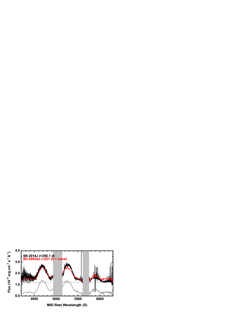
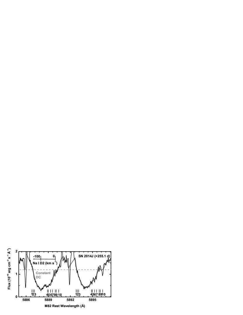
Figure 6.— (Upper panel) Flux-calibrated spectrum of SN 2014J at $+255.1$ days relative to $B$-band maximum brightness, smoothed with a 25 pixel boxcar filter (black). The sky (telluric) lines are not subtracted. CCD gaps are masked by the gray regions. For comparison, a spectrum of the normal SN Ia 2003du at $\sim$221 days relative to $B$-band maximum brightness is also shown (Stanishev et al., 2007), for which the wavelength and the flux are brought to the M82 rest frame (gray, solid). The spectrum of SN 2013du is reddened to match the total extinction toward SN 2014J, $E(B-V)=1.37$ mag and $R_{V}=1.4$. Adding a constant $f_{\lambda}$ continuum (gray, dashed) to the SN 2003du spectrum, the sum (shown in red) is similar to the ‘total’ SN 2014J spectrum. (Bottom panel) The same SN 2014J spectrum focusing on the wavelength region around Na I D (gray). Also shown is the unsmoothed spectrum (black). The dashed line labeled as ‘constant DC’ is the assumed continuum level in the diffuse component, the same as that shown in the upper panel. A velocity scale for Na I D2 in the M82 rest frame is indicated in the lower panel.

Figure 6 shows the flux-calibrated $+255.1$-day spectrum of SN 2014J, following our fiducial reduction procedures. For comparison, the positions of the 10 unsaturated components covering the velocity range from $-160$ to $+23$ km s^-1 in the M82 rest frame, as identified by Graham et al. (2015), are shown. One immediately notices that the spectrum is indeed contaminated by a component (or components) other than the SN itself: At this late-phase, the SN emission is created within the optically thin ejecta, characterized by forbidden lines (from Fe-peak elements for SNe Ia) and virtually zero continuum flux. In Figure 6, this is seen in the spectrum of normal SN Ia 2003du (Stanishev et al., 2007) but reddened using $E(B-V)=1.37$ mag and $R_{V}=1.4$ as derived for SN 2014J (Goobar et al., 2014; Kawabata et al., 2014). Adopting slightly different values for the extinction (Foley et al., 2014) does not change our conclusions. After correcting for the difference in the distances to and extinction within the host galaxies, it is clear that the spectra are quite similar in both the general features and the flux scale, except that there is an offset in the level of continuum. If we add a (roughly) constant flux across the observed wavelength range to the spectrum of SN 2003du, the overall feature of the late-time spectrum of SN 2014J is well reproduced. This shows that nothing peculiar is taking place in our late-time spectrum, but rather that it can simply be interpreted as a sum of the SN and the light from background (or foreground) regions (hereafter the SN-site diffuse component). Note that the flat continuum implies an observed color of $B-V\approx 0.6$ mag, which is roughly consistent with the color of diffuse light in M82 (Mayya & Carrasco, 2009).

The $+255.1$ day spectrum was extracted such that the aperture was chosen to be roughly the slit length, i.e., corresponding to $\sim$2″ of radius (Figures 1 and 4). This translates into a projected physical scale of $\sim$40 pc at the distance of M82 (or $\sim$80 pc in diameter). For comparison, the SN ejecta must have expanded to $\sim$0.02 pc for the ejecta velocity of $\sim$0.1$c$, and the emitting region should be even smaller than this since the light is emitted from the innermost region in the nebular phase. On the other hand, there is a substantial contamination from the diffuse light in our integrated $+255.1$ day spectrum, becoming $\sim$70% of the total light at the wavelength of Na I D (Figure 6). Only a negligible fraction of this diffuse light should subtend the same angle subtended by the SN ejecta, while overall the diffuse light shows the similar Na I D systems to those seen toward SN 2014J in the earlier phases (when contamination by the diffuse light was negligible).

While typically the SN-site diffuse flux can be (and is) neglected for high-resolution observations of SNe (taken around maximum brightness), this is not the case for the last epoch in our observations: the SN flux has decreased substantially at $+255.5$ days, and the SN is in an active starburst galaxy, M82. Indeed, substantial contamination from M82 is inferred from the spatial distribution of the incoming light (Figure 4). A component with a FWHM of $\sim$0.8″ is clearly identified as coming from a point source, and this component is superimposed by another component with a more extended spatial distribution covering at least the length of the slit. The flux ratio between the two components depends on the wavelength, and the contribution from the point source is large where strong emission lines exist in SN Ia spectra at a similar epoch (Figures 4 & 6). Therefore, the point source component is identified as the SN while the diffuse component is likely coming from the diffuse light of M82. This interpretation is further tested below.

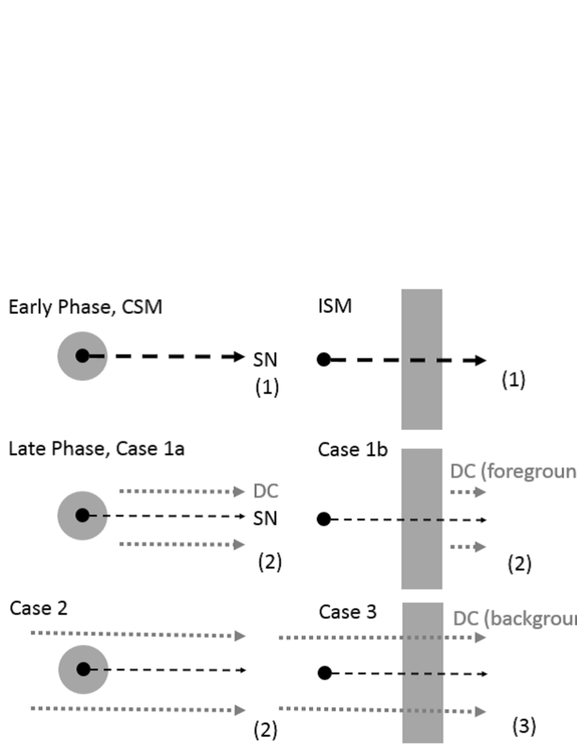
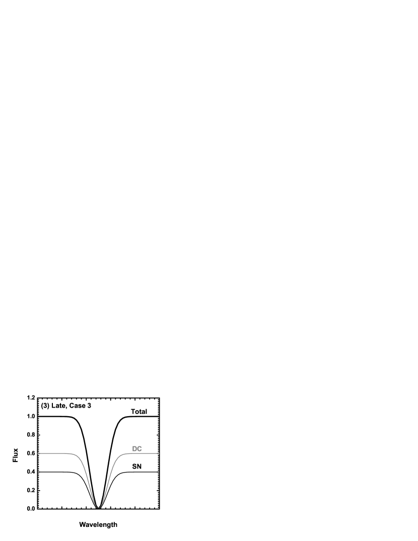
Figure 7.— Sketch of the Na I D absorbing systems toward a point source (SN) with a contribution from an unrelated diffuse component (DC). An example is shown for a single line that is saturated through the absorbing system under consideration, either CSM or ISM. In the early phase, the SN is bright and the contribution from the DC is negligible, and the spectrum is formed by light that goes through the absorbing system as shown in (1). If a large fraction of the DC does not pass through the absorbing system, the absorption-free DC creates the non-zero floor at the bottom of the absorption line at the flux level of the DC even if the line is saturated within the absorbing system, as shown in (2). Finally, if the DC shares the same absorbing system as the SN light, the (flux-normalized) spectra of these two components are the same, and thus the total spectrum, being a combination of the two, is identical to that observed in the early phase, as shown in (3).

We have checked the surface brightness of the region around the SN in a pre-SN image taken with HST/ACS/WCS in the F555W filter (i.e., covering the region containing Na I D), as shown in Figure 1 (Obs ID: 10776, PI: Mountain, see also Crotts, 2015). We estimate that the surface brightness is $\sim$18.3 mag arcsec^-2. Indeed, this is consistent with the typical value of the surface brightness, $\sim$18.5 mag arcsec^-2, in the $V$-band at the position $\sim$60″ away from the center of M82 along the major axis (e.g., Mayya & Carrasco, 2009). If we integrate this diffuse light within the aperture of $0.8\times 3.8$ arcsec² (corresponding to the slit size), a nominal value in our spectral extraction, the contaminating light would result in $V\approx 17.1$ mag, comparable to the expected magnitude of SN 2014J at this phase extrapolated from the early-time light curve (i.e., $V\approx 17$ mag). By performing spectrophotometry on our fluxed spectrum, we obtain $B\approx 16.4$ mag and $V\approx 16.5$ mag, values consistent with the idea that the spectrum is a sum of the SN and the diffuse light with comparable contributions. These arguments are also consistent with the spatial distribution of the incoming light (Figure 4). We note that this photometry is not very accurate, since this procedure assumes point-like sources for both the flux standard star and the target, which is not true for the substantial contribution from the diffuse light. In any case, none of our arguments relies on the absolute flux scale, and thus it does not affect any of our conclusions.

Importantly, while there is non-zero flux at the bottom of the ‘saturated’ components in Na I D (as shown in Figure 5 as well), the bottom of the Na I D features are below the SN-site diffuse light. This is strong evidence that the SN-site diffuse light is also absorbed by the same absorbing features that cause the SN 2014J Na I D profiles (see below). We note that a constant flux of the diffuse continuum light is merely a first-order approximation, and indeed it is better fit by a bluer continuum with the $B$-band flux larger than the $V$-band by $\sim$20–30%. We have checked several continuum models for the diffuse light (constant, linear, parabolic) and confirmed that the uncertainty here would not change our arguments — in all cases the depths of absorptions exceed the continuum level.

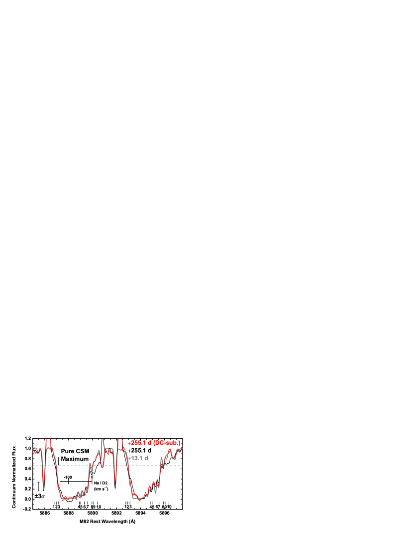
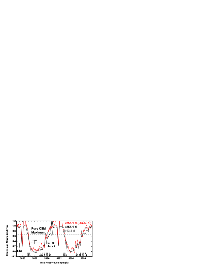
Figure 8.— ‘Contamination-subtracted,’ i.e., the ‘pure SN,’ high-resolution $+255.1$ day spectrum of SN 2014J (red). We also display the total-light spectrum where we have simply subtracted a constant flux spectrum (black) and the $+13.1$ day spectrum (gray). For the aesthetic reasons, all spectra are smoothed with a 7 pixel boxcar filter. Two models for the underlying diffuse component are tested: In Model 1 (upper panel), the off-SN region (at $\sim$0.8″) was subtracted simultaneously when extracting the 1D SN spectrum. In Model 2 (lower panel), the 1D spectrum of the off-SN diffuse component was extracted independently from the SN spectrum extraction within the annuli of 1.4 – 1.9″, and then the flux of this diffuse light spectrum is scaled to fit to the minimum flux of the unsubtracted SN spectrum at the bottom of the (presumably) saturated Na I D components. The resulting contaminating spectrum is then subtracted from the original spectrum. The dashed line marked ‘Pure CSM Maximum’ indicates the maximum depth for a component coming exclusively from the CSM (i.e., along a pencil-like beam toward the SN), where the putative CSM component is assumed to be saturated without any contribution from the larger physical scale (see Figure 7). This is set by the continuum of the DC.

Depending on whether the origin of the contaminating diffuse light is in front of the absorbing cloud(s) (i.e., foreground) or behind it (i.e., background), and on whether the size of the absorbing cloud(s) is smaller or larger than the size of the SN photosphere, there are three situations to consider in discussing the depths of the absorbing components. This is schematically shown in Figure 7. (Case 1: ) The contaminating diffuse light originates in a foreground region. In this case, the spectrum of the SN-site diffuse light is free of absorption and would have a roughly flat continuum. Thus, if the SN line-of-sight absorptions are all saturated, then the maximum depth of the absorbing systems would be at the continuum level of the contaminating light. (Case 2: ) The contaminating diffuse light is behind the absorbing system and the absorbing system is small. In this situation, the contaminating light would not suffer absorption, and again it is simply a continuum. Therefore, the same argument as in Case 1 holds. (Case 3: ) The contaminating diffuse light is behind the absorbing system, and the absorbing system is large. In this case, the depths of the absorbing systems are independent of the contamination of the diffuse light. Generally, the contaminating light can be the sum of light originating in the region in front of the absorbing cloud(s) and light from behind it. However, if the absorbing cloud is small (a combination of Cases 1 and 2), the depths of the absorption can never go below the continuum level. Only if the absorbing cloud is large can the depth of the absorbing system be below the continuum level, and the depth is basically determined by the fraction of the light from the region behind the absorbing system as compared to the foreground light (a combination of Cases 1 and 3).

Therefore, if there are Na I D absorbing systems localized exclusively within a pencil-like beam along the line-of-sight to SN 2014J, the absorption strengths of such components can never be below the continuum level of the diffuse component. All the saturated components are indeed below this level in their fluxes (Figure 6), immediately rejecting the possibility that any of them is associated with a local region around the SN. This also applies to most of the unsaturated components. Except for the unsaturated components 1 and 10, their depths are below the continuum level. Thus the unsaturated components 2–9 should not be associated with the local region around the SN. It is very unlikely that even the remaining components 1 and 10 are from the local SN site. The depths of these components are comparable to the level of the diffuse light continuum, and therefore they must be saturated if there is no corresponding absorption system in the diffuse light. On the other hand, these components were not saturated in the earlier phases, and indeed they were the weakest absorbing components among those clearly identified toward SN 2014J. While this possibility of their being saturated on $+255.1$ days is not strictly rejected from the argument presented here alone, we will show in the subsequent sections that this possibility is very unlikely.

3.3. Have the Intrinsic SN Absorbing Systems Changed?

Despite our conclusion that all the visible components of the Na I D systems toward SN 2014J are shared by a diffuse light from the region extending to $\sim$80 pc in the projected diameter, this does not readily reject the possibility that some components might contribute (although not predominantly) via local CSM components around SN 2014J. The first point to clarify regarding this issue is whether there is variability in the absorbing spectrum along the ‘pure’ line-of-sight to SN 2014J. For this purpose, we try to subtract the contribution from the unrelated diffuse component to extract the pure, contamination-subtracted SN spectrum. In addition to investigating the temporal variability in the SN line-of-sight spectrum, this procedure inversely provides a check on our conclusion that there is a substantial contamination from the unrelated diffuse light to the SN spectrum as we will show below.

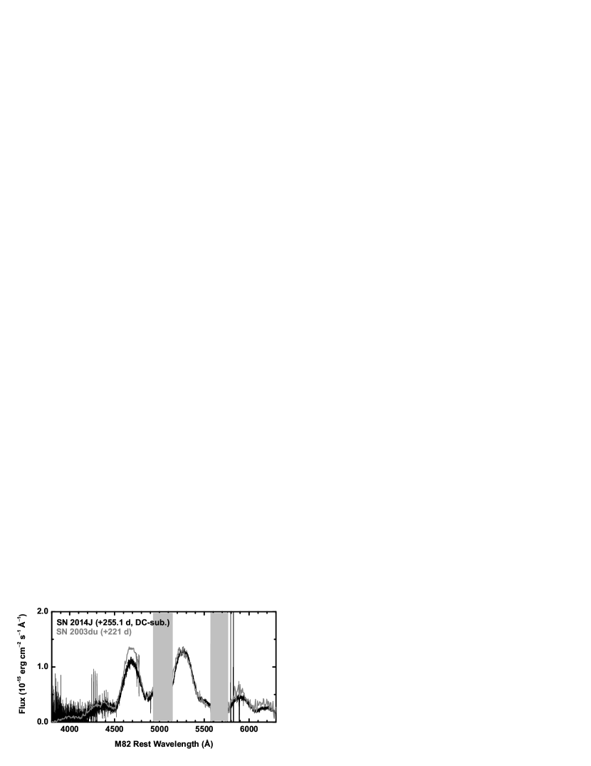
Figure 9.— Same as Figure 6 (the flux-calibrated spectrum of SN 2014J), but after subtracting the diffuse component using the DC model 1. In the upper panel, a spectrum of SN Ia 2003du at $\sim$221 days is also shown (gray; distance and extinction “corrected” for to match those of SN 2014J). In the bottom panel, the smoothed (gray) and unsmoothed (black) spectra are shown for the wavelength region covering Na I D1 and D2.

We created a model spectrum of the contaminating diffuse light and subtracted it from the original target spectrum. For this purpose, we tested two SN-site contamination models. In the ‘DC (diffuse component) model 1,’ the contaminating diffuse light was subtracted simultaneously when extracting the 1D SN spectrum using the apall task in IRAF. In doing this, we extracted the SN flux within an aperture of $\sim$0.8″ $\times$ 0.8″, and the contaminating light was fit by a linear function connecting the regions $\sim$0.8″away from the SN along the slit. In the ‘DC model 2’, we extracted 1D spectra for regions $\mathrel{\hbox to0.0pt{\lower 4.0pt\hbox{\hskip 1.0pt$\sim$}\hss}\raise 1.0pt\hbox{$>$}}$1.4″away from the SN position (in both directions) along the slit (see Figures 1 & 4). The spectra of the contaminating diffuse light obtained for both sides of the target (North and South) were then averaged. The flux of this contaminating spectrum was scaled to fit to the minimum flux of the unsubtracted SN spectrum, extracted within $\sim$1.4″ from the SN position, at the bottom of the saturated Na I D components. Then the contaminating spectrum was subtracted from the unsubtracted SN spectrum, resulting in a ‘pure’ SN spectrum. Note that the contaminating spectrum, in both models, will contain some SN light (given that the DC extraction regions are relatively close to the SN position as compared to the seeing size of $\sim$0.8″), and thus it is not a spectrum of only the contaminating diffuse component. In any case, since both the target spectrum and the diffuse component spectrum contain the pure SN and pure diffuse light spectra, the subtraction should yield a pure SN spectrum.

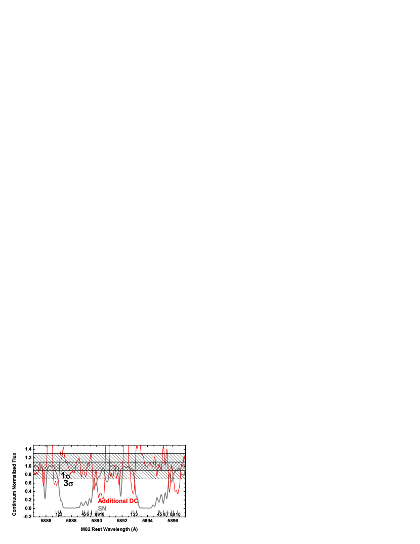
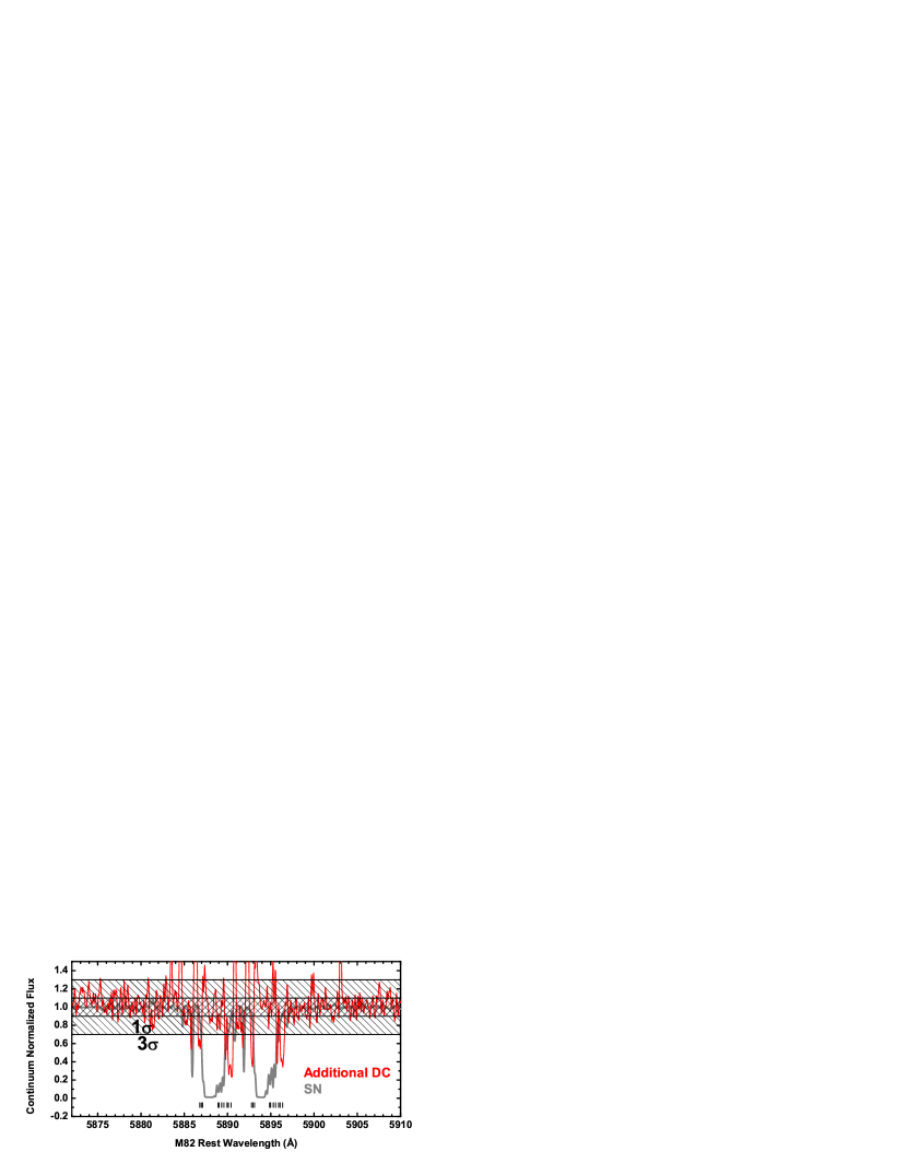
Figure 10.— Difference between the $+255.1$ day total (diffuse-light contaminating) spectrum and the $+13.1$ day SN 2014J spectrum (red curve). The original spectrum is deconvolved into the SN component and this additional DC, and the resulting ratios (in the continuum flux) are $\sim$75% and $\sim$25%, respectively. This residual spectrum has been smoothed with a 7 pixel boxcar filter. Shown in gray is the Na I D profile for reference. The gray hashed regions represent 1 and 3-$\sigma$ deviations between the SN and diffuse component. The lower panel shows an extended view in the dispersion direction to show the noise level of the resulting spectrum.

Figure 8 shows the resulting ‘pure’ SN spectrum, normalized by the continuum. While the S/N per pixel is reduced to $\sim$15 – 18 in the continuum around the Na I D (after the binning of 7 pixels), we find that the resulting contamination-subtracted line profiles are consistent with those in the spectra from earlier phases. No significant variation between the early- and late-time spectra is found any longer beyond $3\sigma$. This is clearly seen in the blue and red wings of the saturated components where the unsaturated components are present (i.e., components 1–3 in the blue and components 8–10 in the red). In particular, the spectral slopes in the blue and red parts of the saturated components (blueward of component 1 and for the wavelength region around component 10), originally flatter (deeper) than those in the earlier phases, are now steeper (shallower) than the original (unsubtracted) spectrum, and consistent with those at early phases. The facts that this is confirmed irrespective of the model for the contaminating diffuse light spectrum and that it is seen in both of the D1 and D2 lines strongly support this conclusion. Therefore, we conclude that the Na I D absorbing systems in the ‘pure’ SN spectrum, i.e., those exactly along the line-of-sight to SN 2014J (here within the projected radius of the size of the SN at this phase, i.e., $\sim$0.02 pc), did not change significantly even $+255.1$ days after $B$-band maximum brightness.

This also supports the idea that ‘all’ absorbing systems are dominated by giant absorbing clouds in front of the SN site. In §3.2, we mentioned that, strictly speaking, components 1 and 10 could potentially come from the region localized to the SN position (i.e., ‘CSM’). If these components, originally weak in the early phases, became saturated on +255.1 days, then it is possible that these components are truly local to the SN without any contribution from foreground systems. However, if this is correct, we should see these components nearly saturated in our ‘contamination-subtracted’ spectrum, but this is indeed the opposite of the observations. Therefore, this possibility is rejected, and we conclude that all absorption systems are dominated by those in the foreground.

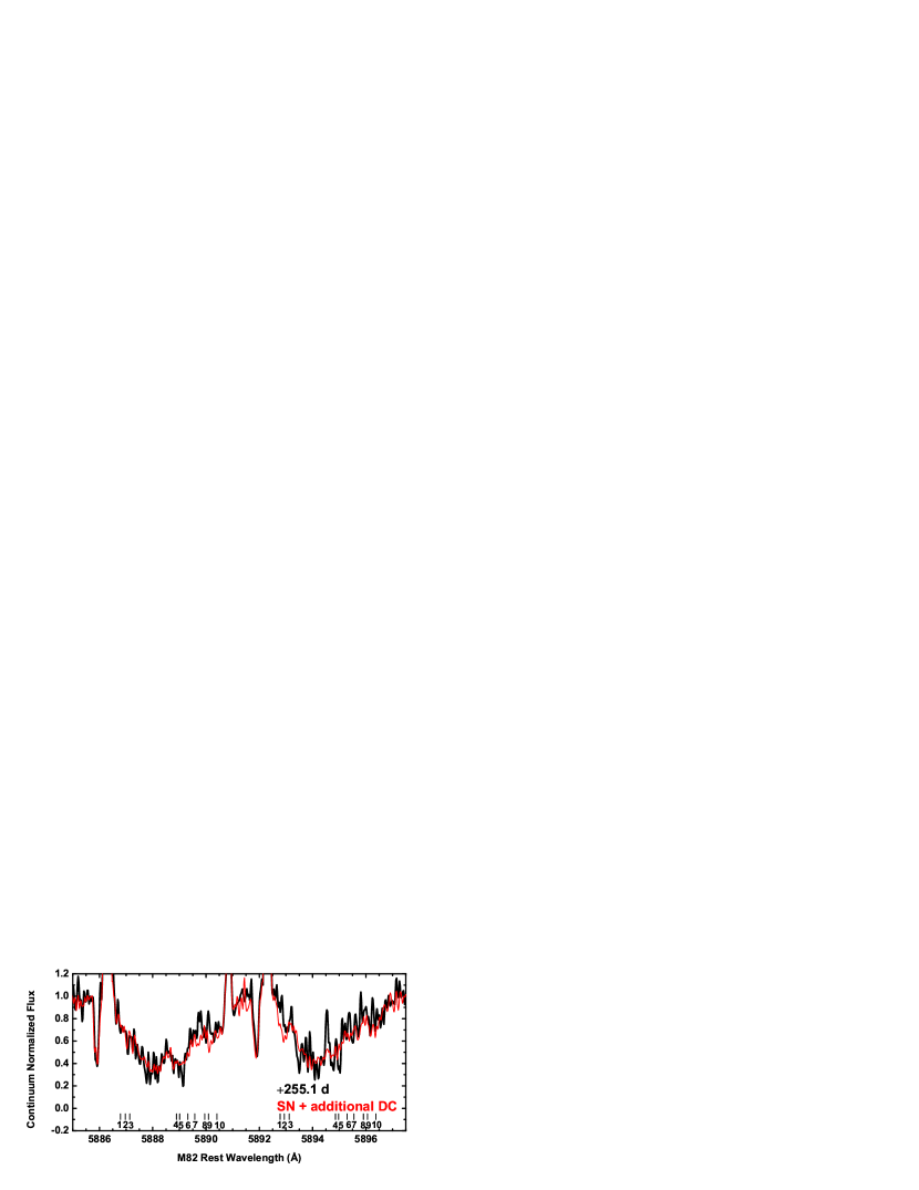
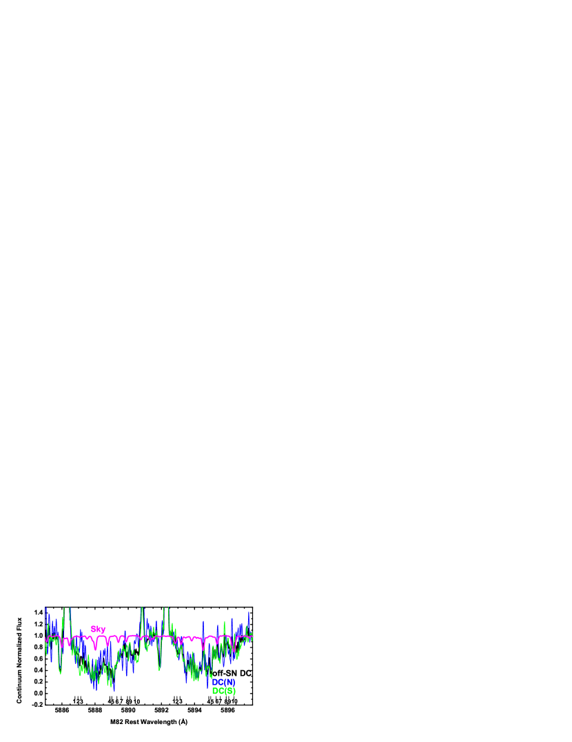
Figure 11.— (Upper panel) Spectrum of the off-line-of-sight region, averaging the north and south regions (black: see Figure 1). The red curve represents a reconstruction of this spectrum by combining the SN-only and DC components considered in Figure 10. The relative contributions to the continuum flux are 60% from the SN component and 40% from the pure (additional) diffuse component. Note that the relative contributions of these pure SN and DC components in this off-line-of-sight spectrum are different from those in the line-of-sight spectrum (see the Figure 10 caption). (Lower panel) North (blue) and South (green) background spectra as well as the averaged spectrum (black). The sky spectrum is also shown (magenta).

Another check on our conclusion can be provided by performing the flux calibration to the contamination-subtracted pure SN spectrum. This is shown in Figure 9 for the DC model 1. After the correction, the SN shows no additional flux, and this pure SN spectrum provides a good match to a spectrum of SN 2003du at a similar epoch. Also, the depths of the absorption are now consistent with that seen in the early phases, reaching to the zero-flux level in the saturated components. All of these features support our interpretation.

3.4. Spatial Variation in the Absorbing Systems

The SN-site diffuse light globally shows a similarity to that directly along the line-of-sight to SN 2014J, and therefore the bulk of the absorbing systems are in the foreground region. However, we have not yet quantitatively demonstrated that the absorbing systems for the diffuse light and SN are exactly identical. Given the lack of temporal variation in the ‘pure’ SN component, the apparent difference between the early-time and late-time (diffuse light-contaminated) spectra means that there must be a difference between the ‘pure’ SN and the diffuse components, otherwise the sum must be always identical.

We assume that the pure SN component in the late-time spectrum is identical to that in the earlier phases, and subtract it from the original, diffuse light-contaminated late-time spectrum (the ‘total’ spectrum in Figure 1). We note that this procedure also subtracts the diffuse light that has an absorption-line spectrum identical to the pure SN spectrum. Namely, if the SN and the diffuse light (within the aperture of $\sim$40 pc in radius) show exactly the same absorption systems, there should be no residuals. We note that this procedure is identical to one examining the time variability of the absorption systems toward an SN. However, given our conclusion that basically all of the absorbing systems are located far from the SN in the foreground region (having a physical scale of $\mathrel{\hbox to0.0pt{\lower 4.0pt\hbox{\hskip 1.0pt$\sim$}\hss}\raise 1.0pt\hbox{$>$}}$40 pc in radius), we regard any residuals, if they exist, as originating in the ‘spatial’ variation (within $\sim$40 pc in the radius).

The result of this exercise is shown in Figure 10, which shows a spectrum of ‘additional’ absorbing components after the ‘pure’ SN spectrum has been subtracted from the total spectrum. Inversely, we find that the relative contributions in the total light are $\sim$75% (the pure SN + the identical diffuse component) and $\sim$25% (the additional diffuse component superposed on the continuum) in the continuum flux. The relative contribution reflects the depth of the ‘saturated’ components in the total light, which is $\sim$25%. Using this information, we can infer the origin of the contaminating light either in the region in front of the absorbing system (i.e., foreground) or behind it (i.e., background): here, the contribution to the total light within the whole aperture from the foreground light must be $\sim 25$%, and the remaining $\sim 75$% being the sum of the SN light and the diffuse light, must come from the region behind the absorbing cloud(s).

Features in the derived residual spectrum can be interpreted as follows. First, in most of the wavelength range across the Na I D absorption, the difference is within $3\sigma$. Therefore, the majority of the absorbing systems are identical between the line-of-sight to the SN and the off-line-of-sight (beyond $\sim$0.02 pc from the SN center in projected radius). Of course, we cannot quantify the difference in terms of the column density for the saturated components, but there is no hint that the column density in the off-line-of-sight is significantly smaller than that along the line-of-sight. This strengthens our conclusion that the absorbing systems are produced by foreground materials located between the SN and us, extending to the scale of $\sim$40 pc in the projected radius. As for the unsaturated components, numbers 3–8 show residuals within $3\sigma$, showing no significant difference between the SN and the diffuse component. Therefore, these regions must not have significant variation across the projected radius of $\sim$40 pc, suggesting these components, together with the saturated components, are attributed to a giant cloud of absorbing matter extending more than 40 pc in the physical scale. Note that these are the systems showing the largest absorption (therefore a low flux level), and thus the S/N ratio is quite low. Indeed, there is a hint that components 3 (and blueward) and 7 show ‘negative’ additional absorption, but given the relatively low S/N ratio in this spectrum of the additional diffuse component (Figure 10), this is just indicative.

There are some absorption systems that vary beyond $3\sigma$: the unsaturated components 1 ($-160$ km/s relative to the M82 rest frame), 2 ($-152$ km/s), 9 ($+7$ km/s), and 10 ($+3$ km/s). There is also a significant absorbing system at the wavelength between the components 7 ($-19$ km/s) and 8 ($0$ km/s) where the SN line-of-sight does not show significant absorption. In addition to the statistical significance, these are all seen in both Na I D1 and D2, and therefore these features must be real. These should be components whose column densities vary depending on the line-of-sight, within a scale of $\sim$40 pc in projected radius. It is interesting to see that the components showing the spatial variation are the systems having weaker absorption (thus smaller column densities) than those showing no variation. This may suggest that the spatially smaller systems tend to have lower column density, which might support our interpretation since the larger systems are expected to have a larger extent along the line-of-sight resulting in a larger column density.

3.5. Further Support for the Interpretation

If our interpretation is correct, it is expected that the spectrum of the diffuse light originates from the region off the line-of-sight to the SN (i.e., that extracted from the region at $\mathrel{\hbox to0.0pt{\lower 4.0pt\hbox{\hskip 1.0pt$\sim$}\hss}\raise 1.0pt\hbox{$>$}}$1.4″) can be reproduced by a sum of the ‘pure-SN’ component and the ‘additional-DC’ component, but with relative contributions different from those applied to the total integrated spectrum including the SN line-of-sight. For the total spectrum, the relative contributions are 75% (the pure SN + the identical DC) and 25% (the additional DC superposed on the continuum) in the continuum flux.

Figure 11 shows that the off-line-of-sight spectrum is well reproduced by a combination of the pure SN (including the diffuse component identical to the SN absorbing systems) and the additional DC components (including the continuum flux), but with different contributions than those applied to the total integrated spectrum. The diffuse spectrum in the surrounding region, as obtained by the DC model 2, is representative of the spectra in the annuli surrounding the SN at $\sim$1.4 – 2″ (i.e., $\sim$30 – 40 pc in projected radius). In this figure, the model spectrum is created by adding the pure SN and the additional DC spectra with relative contributions to the continuum flux of 60% and 40%, respectively. The contribution of the additional diffuse component is increased in the surrounding region. This strengthens our conclusion that the absorbing systems are all from the foreground big system (extending in the spatial scale of $\mathrel{\hbox to0.0pt{\lower 4.0pt\hbox{\hskip 1.0pt$\sim$}\hss}\raise 1.0pt\hbox{$>$}}$80 pc in diameter). We emphasize that the additional DC was created from the whole region extending to $\sim$2″ of the aperture where a large fraction of light is within $\mathrel{\hbox to0.0pt{\lower 4.0pt\hbox{\hskip 1.0pt$\sim$}\hss}\raise 1.0pt\hbox{$<$}}$1.4″. Therefore there is no reason to expect that the off-line-of-sight region ($\sim$1.4″ – 2″) spectrum is explained by the combination of the pure SN and the additional DC at the SN position, if this additional component is attributed to anything else (e.g., time-varying absorption along the SN line-of-sight).

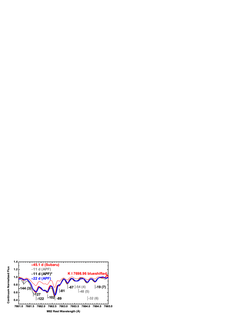
Figure 12.— Continuum-normalized spectrum of SN 2014J at $+45.1$ days relative to $B$-band maximum brightness, shown for the K I doublet ($7664.90$Å in thick-red and $7698.96$Å in thin-red). The red ($7698.96$Å) component is artificially blueshifted in wavelength, so that it is shown in the wavelength scale of the blue ($7664.90$Å) component. The K I components identified by Graham et al. (2015) are marked with black vertical lines, while others corresponding to the Na I D components are marked with gray vertical lines. The numbers denote the blueshift in km s^-1, while those in parenthesis indicate the corresponding Na I D component numbers. The continuum-normalized spectra of the first and last spectra obtained by the Automated Planet Finder (APF) at Lick Observatory (Graham et al., 2015) are shown (one at $-11$ days in thin-gray and at $+22$ days in thick-blue), where the fringing pattern (see the main text) was reconstructed using the same spectrum. Also shown is the result adopting a second fringe correction model for the $-11$ day spectrum (thin-black).

The same argument can be rephrased in a slightly different way. The contribution from the background light (i.e., that from the region behind the absorbing systems) reflects the depth of the ‘saturated component’, which is $\sim$40%. This means that in the off-SN region, the contribution of the light from the foreground (in front of the absorbing cloud) is $\sim$40% with the rest coming from the region behind the absorbing cloud. As the SN light contamination must be negligible along the line-of-sight for this off-SN region to a first approximation, this means that generally near the site of SN 2014J, $\sim$60% of the light is a true background (behind the absorbing systems) and $\sim$40% is a foreground (in front of the absorbing systems).

This is consistent with the contribution of the foreground light reaching $\sim$30% in the total light within the aperture (i.e., the SN and DC), as inferred from the flux of the ‘saturated’ components of Na I D. The SN must be fully behind the absorbing systems, and the SN contribution within the aperture is $\sim$25% in the continuum around Na I D (see Figure 4). Then the contribution from the foreground to the total light should be $\sim$(1 – 0.25) $\times$ $0.4\approx 0.3$, i.e., $\sim$30%.

Because of the image rotation during the exposure, we lose information on the angular distribution of the incoming light around the center of the pointing to some extent (Figure 1). Given the relatively low flux in the off-SN diffuse light (i.e., DC model 2), we have created the off-SN diffuse light spectrum by averaging those on both side of the SN position. However, it is still possible to use some spatial information. Figure 11 shows the spectra of the two spatially distinct off-SN diffuse regions (N, north, and S, south) separately. The spectra of these two regions generally match one another quite well, supporting the idea that the absorbing systems are from the foreground with a physical scale of $\mathrel{\hbox to0.0pt{\lower 4.0pt\hbox{\hskip 1.0pt$\sim$}\hss}\raise 1.0pt\hbox{$>$}}$40 pc in radius. However, there are marginal differences between the two, especially near the unsaturated component 3 (slightly blueward) and the red part of component 10. The former is not seen in Na I D1, but that wavelength overlaps with a relatively strong telluric absorption. The former corresponds to the ‘additional DC’ where the ‘negative’ absorption is marginally seen, and the latter corresponds to the wavelength where the additional DC absorption is detected (Figure 10, upper panel). These indicate that these components show relatively small-scale fluctuations within $\sim$30 pc.

3.6. K I and DIBs

Here we examine the claim by Graham et al. (2015) of variability in the K I profile corresponding to the unsaturated Na I D component 3 ($-144$ km s^-1) and part of the saturated component ($-127$ km s^-1). We have only one spectrum covering the wavelength of K I, but this spectrum is of very high quality and was taken on $+45.1$ days, about 23 days later than the last spectrum presented by Graham et al. (2015). In addition, we note that the spectra taken by the Automated Planet Finder (APF) at Lick Observatory (Graham et al., 2015) to some extent suffer from a fringing pattern in defining the continuum, and thus we want to provide a check with data taken by another instrument. In doing this, we tried to correct for the fringing pattern in the spectra of Graham et al. (2015) using our Subaru/HDS spectrum on $+45.1$ days, which is free from such a fringing pattern. Details are described in Appendix B.

Figure 12 shows the comparison, where our spectrum on $+45.1$ days is compared with the APF spectra at $-11$ days and $+22$ days after correcting for the fringing pattern. First, even without the correction for the fringing pattern, we find that the features in K I on $+45.1$ days are generally in good agreement with those at $+22$ days presented by Graham et al. (2015). The absorption depth of the component at $-144$ km s^-1 is no deeper than $0.9$, and the depth of the component at $-127$ km s^-1 is significantly shallower than that at $-122$ km s^-1. In addition, the same features are confirmed in the red component of the K I doublet in our spectrum. This supports the idea that the features of K I in the APF spectrum at $+22$ days as reported by Graham et al. (2015) are real, and indicates that the features did not show significant variability between $+22$ and $+45.1$ days.

After removing the fringing pattern in the APF spectra, we find an excellent match between the spectra at $+22$ days and $+45.1$ days. No significant evolution is found between the two epochs. The spectra at $-11$ and $+22$ days, with our best effort to correct for the fringe pattern using our Subaru spectrum, reproduce the time evolution found by Graham et al. (2015): at the later epoch, the component at $-144$ km s^-1 became shallower, and the component at $-127$ km s^-1 became shallower as compared to the one at $-122$ km s^-1. Thus, we have confirmed the main findings of Graham et al. (2015) on the variability in K I. In addition, our new spectrum shows that no evolution is seen from $+22$ days to $+45.1$ days.

A question then is how the K I variability is consistent with our finding that all the absorbing systems seen in Na I D are caused by foreground absorbers extended at a scale of $\mathrel{\hbox to0.0pt{\lower 4.0pt\hbox{\hskip 1.0pt$\sim$}\hss}\raise 1.0pt\hbox{$>$}}$80 pc, with a significant fluctuation in the column density for some relatively weak unsaturated components at a scale of $\sim$20 pc. Graham et al. (2015) estimated the distance of the foreground absorbing material, showing the K I variability as being at 3–9 pc from the SN site. Their finding is consistent with our conclusion if the gas is relatively close to the SN but spatially extended in the plane of the sky. It is interesting that we do see a hint of spatial variation in the Na I D absorbing systems within $\sim$20 – 30 pc corresponding to those systems showing the temporal variability in K I (Figures 10 and 11). This supports the origin of this component at a scale of $\sim$10 – 20 pc from the SN in the foreground region. It is notable that the closest material to the SN also has the highest blueshift.

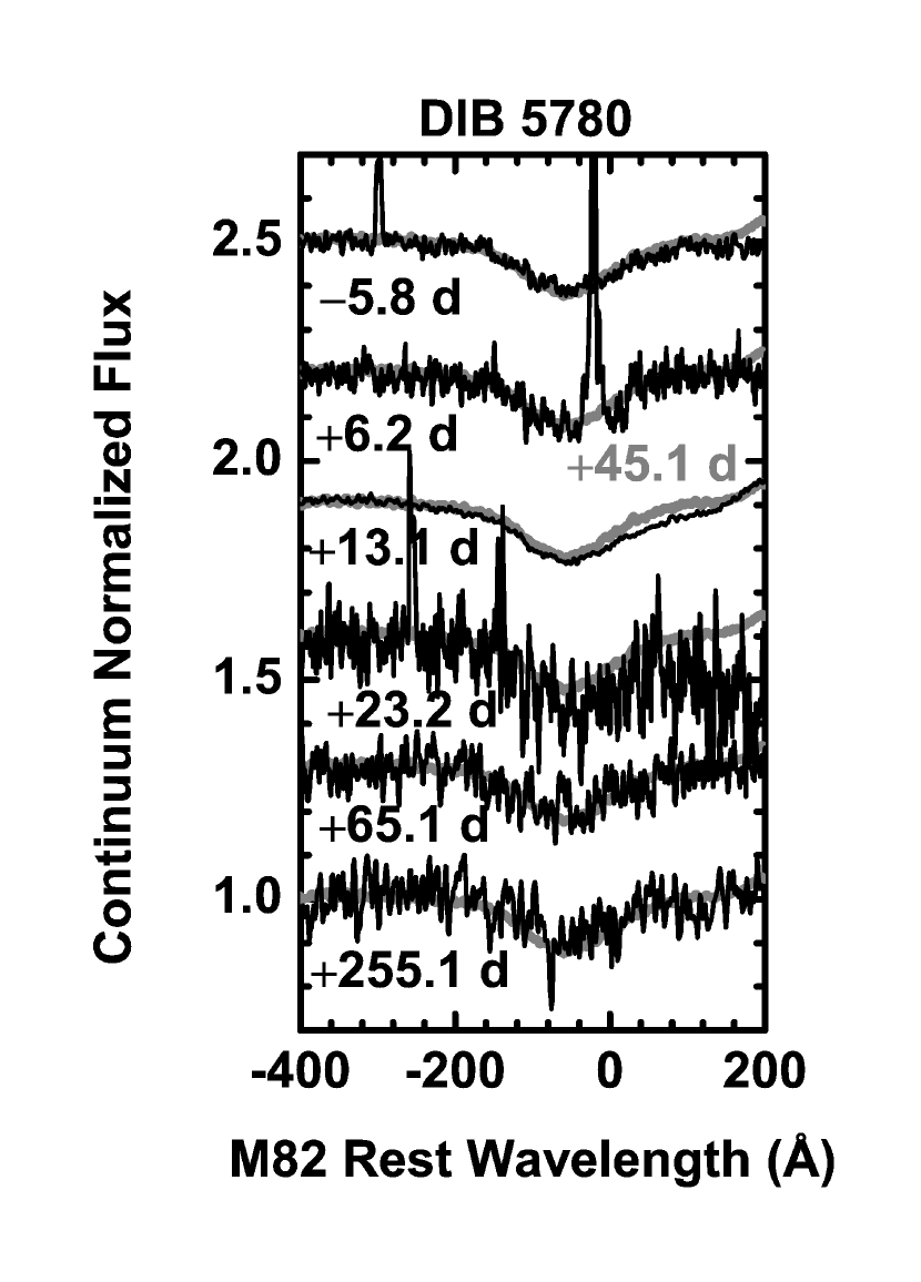
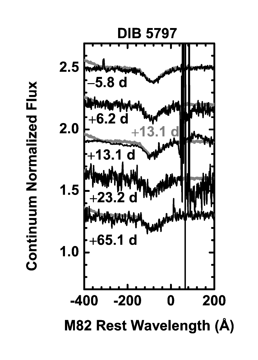
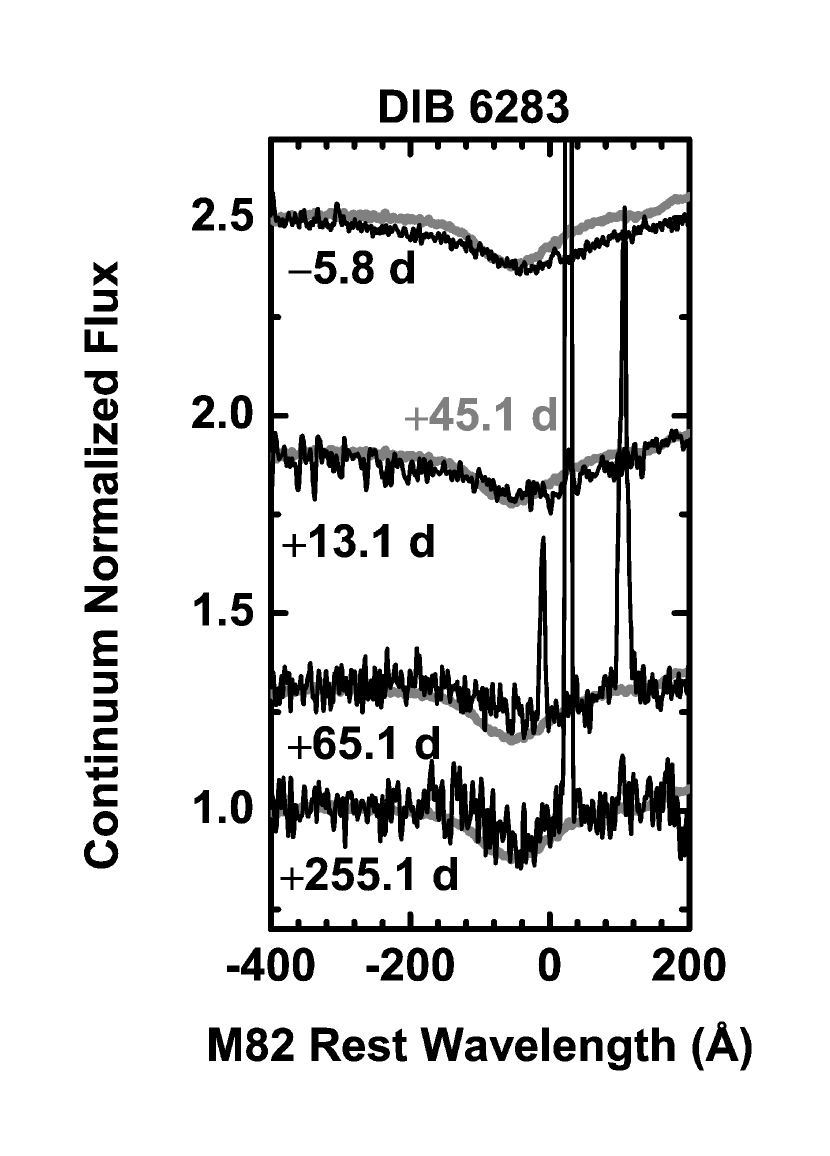
Figure 13.— Spectra focusing on DIB features. The 5797 Å DIB in the $+255.1$ day spectrum falls in a CCD gap. The 6823 Å DIB feature is too noisy in the $+6.2$ and $23.2$ day spectra and is not displayed here.

No significant variation of DIBs has been reported between $-10$ and $+45$ days (for DIBs 5780 and 5797: Foley et al., 2014) and between $-10$ and $+22$ days (DIBs 5780, 5797, 6196, 6283, 6613: Graham et al., 2015). Figure 13 shows the evolution of DIBs in our spectra, up to $+255.1$ days for DIBs 5780 and 6283, and up to $+65.1$ days for DIB 5797. While the analysis of DIBs is limited by the S/N ratio and the accuracy of the continuum subtraction, no significant variation is seen for these features up to $+255.1$ days. This is consistent with the idea that the DIBs mainly originate in the ISM (van Loon et al., 2009, 2013), and thus the existence and strengths of DIBs can be used to trace the ISM components and extinction toward SNe (Phillips et al., 2013). Interestingly, this result provides a good contrast to variation in some DIBs reported for broad-lined SN Ic 2012ap associated with the death of a massive star (Milisavljevic et al., 2014). While the equivalent widths of DIBs are comparable for SNe 2014J and 2012ap, no variation is seen for SN 2014J even at $+255.1$ days (note that this study presents the longest span so far for any SNe for which such an evolution in DIBs has been tested). It highlights the difference between SNe Ia and core-collapse SNe, and may shed light on the still enigmatic origin(s) of DIBs.

4. Conclusions and Discussion

We have discovered apparent ‘variability’ of some the Na I D absorption systems toward SN 2014J. We however conclude that this variability does not reflect intrinsic time variability of the absorbing system along the line-of-sight toward the SN, but rather reflects the contamination of an unassociated diffuse light whose contribution was negligible when the SN was bright. Indeed, we note that the similar behavior might have been already seen previously in the spectrum of SN 2007le at $+90$ days (Simon et al., 2009); which might have been caused by bad seeing in the observation leading to a contamination of an off-SN site diffuse light to the true SN spectrum in that case. The diffuse light contamination, usually an obstacle in isolating the properties of the line-of-sight information toward an SN, however turns out to be very powerful in identifying the origin of the strong and complicated absorbing systems seen in SN 2014J. Specifically, this study presents the first case where all absorbing systems toward an individual SN are unambiguously deconvolved into ISM and CSM components (resulting in no CSM components for SN 2014J) – Extraction of the CSM components has been successful either using time variability for individual objects (e.g., Patat et al., 2007; Simon et al., 2009) or using a large number of SNe for a statistical sample (e.g., Sternberg et al., 2011). However, both routes ineitably lack the identification of the origin(s) of the non-variable components for individual SNe.

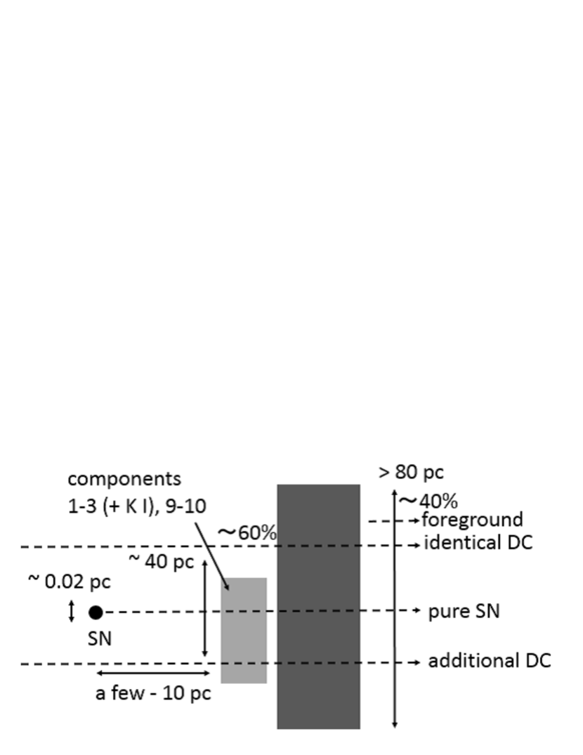
Figure 14.— Sketch of the Na I D absorbing systems toward SN 2014J.

The inferred structure of the absorbing systems is schematically shown in Figure 14. All absorbing systems seen toward SN 2014J should be located in a foreground region far from the SN site since they show the depths of the absorption clearly exceeding the value expected for a system localized along the SN line-of-sight (§3.2 and Figure 7). That is, the absorbing spectrum of the contaminating light is generally identical to that intrinsically toward the SN (i.e., within $\sim$0.02 pc of a pencil beam toward the SN). The physical scale of the absorbing system must be (generally) greater than $\sim$80 pc because the spectrum does show generally identical absorbing systems at this scale. The ‘saturated’ components show a non-zero flux at a level of $\sim$30% relative to the continuum, and it is likely that this is caused by a contamination from the foreground region with respect to the location of the bulk absorbing materials. The intrinsic (without SN) contribution of the foreground light reaches $\sim$40% near the SN site.

Identifying the diffuse light contamination, we have managed to subtract this from the total light and have extracted a ‘pure’ absorbing spectrum toward the SN. This pure line-of-sight spectrum does not show significant change in the strength of the absorbing systems as compared to the spectra at earlier phases. Namely, the intrinsic line-of-sight absorbing systems within a narrow line-of-sight toward the SN did not change even at $+255.1$ days. This is in accordance with our conclusion that all of the visible absorbing systems are located far from the SN site and not at close to the SN (i.e., not CSM).

At the same time, we see small, but significant, differences in the absorbing systems in the late-time spectrum (SN plus the diffuse light) and in the earlier phases. The difference is seen in some unsaturated components. Since there is no evidence for temporal variability along the SN line-of-sight, this variation must come from the ‘spatial’ variation at a scale of $\mathrel{\hbox to0.0pt{\lower 4.0pt\hbox{\hskip 1.0pt$\sim$}\hss}\raise 1.0pt\hbox{$<$}}$40 pc in projected radius. This is further supported by the fact that this difference strengthens at larger radii.

Another appealing possibility, not mentioned in §3, is that this apparent variation in the spatial dimension might reflect a light echo, where the SN light is scattered off dust sheets to us. A projected light echo position can show a superluminal motion and thus can extend to the projected distance of $\mathrel{\hbox to0.0pt{\lower 4.0pt\hbox{\hskip 1.0pt$\sim$}\hss}\raise 1.0pt\hbox{$>$}}$20 pc. If this is true it would indicate an angle-dependent inhomogeneity in the absorption systems, but we regard this possibility as highly unlikely. Crotts (2015) reported that diffuse components appeared at about $+213$ days in the HST image, associating them with the SN light echo. The components are however much fainter than the SN itself, and thus this would not explain the apparent difference in the absorption-line spectra in the earlier epochs and that at $+255.1$ days. Our flux-calibrated spectrum at $+255.1$ days shows a normal SN Ia nebular spectrum, showing no clear signature of a light echo. We note, however, that the continuum of the SN-site diffuse light is relatively blue, and it may indicate that there could possibly be some contamination from an SN light echo there. While the contamination would not be at a level to change our conclusions, investigating the possible unresolved light echo component itself is an interesting topic and continual follow-up observations of SN 2014J are highly encouraged.

We confirmed the finding of Graham et al. (2015) for the variability of K I, but also extended the analysis to a later epoch. The nature of variable K I components, at $-144$ km s^-1 and $-127$ km s^-1 (with respect to the M82 rest frame), in the $+45.1$ day spectrum is consistent with that at $+23$ days, indicating that those components have stabilized after $+23$ days. Given the conclusion by Graham et al. (2015) that the system is likely located at a distance of 3–9 pc from the SN, this does not conflict with our findings regarding the Na I D absorption systems – they are both in the foreground region. DIBs did not show significant evolution from $-5.8$ days to $+255.1$ days, further supporting the location of the absorbing system being far from the SN site.

The derived configuration is consistent with the HST high-resolution pre-SN image (see Fig. 1). SN 2014J is in the region where a dark lane is seen, and the region typically shows a fluctuation in the surface brightness at a scale of $\sim$20 pc.

While we do not constrain the line-of-sight distance between the SN site and the absorbing materials (e.g., suggested to be 3–9 pc for the highest-velocity clouds as determined from the K I variability: Graham et al., 2015), we do constrain the projected size of the systems as being at least $\sim$40 pc. Therefore, if the absorbing material is related to pre-SN activity, then it had to affect a large distance ($\sim$40 pc) rather than a few pc. This implies that it is unlikely that the absorbing material is directly related to progenitor activity.

To quantify this point, we divide the question into two sub-parts. The first question is whether there is any possibility that the absorbing materials at this distance can be explained by material ejected from the SN progenitor system – the answer is no. If the SN progenitor had affected a region of this size ($\sim$40 pc in radius), assuming spherical symmetry, the swept-up materials from the ISM would have to be as large as $\sim$6000 $M_{\odot}(n_{\rm ISM}/1\ {\rm cm}^{-3})$, greatly exceeding ‘CSM’ material ejected from any proposed systems for SNe Ia. The next question is whether there is a chance that this region was affected by the progenitor system activity – the answer is that it is possible but not likely, as highlighted below when considering cases expected from the SD scenario.

If this material has been accelerated by a wind from a red-giant companion star with $10^{-6}M_{\odot}$ yr^-1 and a wind velocity of $\sim$30 km s^-1 (i.e., an extreme case of the symbiotic path in the SD scenario), namely at a power of about $3\times 10^{32}$ erg s^-1, it would take about $2\times 10^{7}$ years for the swept-up materials to reach $\sim$40 pc. In this case the expected expansion velocity should have decreased to a few km s^-1, even if radiation energy loss from the expanding shell is ignored. This suggests that the ISM expansion caused by the hypothesized companion giant wind would not reach this large spatial extent. In a symbiotic case within the SD scenario, the ISM-shell expansion might be further energized by recurrent nova activities. If the system emitted a kinetic energy of $\sim 10^{43}$ erg in each eruption with a recurrence time of $\sim$10 years, then the averaged kinetic input to the surrounding ISM would be about $3\times 10^{34}$ erg s^-1. In this case, the swept-up ISM would take about $5\times 10^{6}$ yrs to reach $\sim$40 pc. The resulting expansion velocity would be $\sim$10 km s^-1. This possibility is not rejected, but then the bulk kinematics seen in the absorbing systems (reaching to about $-150$ km s^-1 for the component showing the variability in K I) must be attributed to the ISM kinematics unrelated to the shell expansion. At this point, the line velocity cannot be explained by a wind. The largest impact on the gas surrounding the SD progenitor system would be expected by an optically thick accretion wind, which would have a kinetic power four orders of magnitude larger than the red-giant companion wind. In this case it would take about $10^{6}$ yrs for the ISM shell to reach $\sim$40 pc, and the resulting expansion velocity would be $\sim$50 km s^-1. This is probably the only scenario, within the hypothesis that the absorbing systems are directly related to the progenitor, that could account for the kinematics of the blueshifted absorbing systems. However, in this case, we would expect to see a supersoft X-ray source in pre-explosion images, while none was detected (Nielsen et al., 2014).

To push the above arguments further, we point out that it is generally difficult to explain the kinematics of the absorbing system toward SN 2014J as merely coming from the SN progenitor system, irrespective of any assumptions about the system. This requires an excessively large kinetic power input from the progenitor system. It is naturally expected that such an energy input may well be followed by electromagnetic radiation at some wavelength, while there were no detections of such a source in pre-explosion images (Goobar et al., 2014; Nielsen et al., 2014; Kelly et al., 2014). Therefore, the absorbing systems towards SN 2014J should have no direct relation to the SN progenitor system activity.

The non-detection of radio and X-ray signals from the putative SN ejecta-CSM interaction places a strong constraint on the amount of the CSM around the SN within $\sim$0.01 pc (Pérez-Torres et al., 2014; Margutti et al., 2014). Properties of the polarization, especially the non-detection of time variability, imply that the source of the polarization is in the ISM (Kawabata et al., 2014; Patat et al., 2015, although, see Hoang 2015). No NIR/IR echo has been identified for SN 2014J, which places a strong upper limit on the amount of CSM (Johansson et al., 2014) (see also Maeda et al., 2015, for a light echo model and constraints for SNe Ia in general). Finally, the present study shows that all observed narrow-line absorptions likely originate from material in the ISM. Strictly speaking, our analysis does not reject the possible existence of CSM around SN 2014J, but it does reject any association of the observed (narrow) absorbing systems with such CSM. There are indeed suggestions that the extinction curve toward SN 2014J is better explained by a ‘multiple scattering model’ (Goobar, 2008; Amanullah et al., 2014) than the ISM dust model, and that the non-standard extinction curve toward SN 2014J could be explained by a combination of ISM and CSM components (Foley et al., 2014) (but see Amanullah et al., 2015). We have not yet arrived at a unified explanation for all of these constraints, but our result adds to another strong constraint on the existence of CSM.

To our knowledge, this is the first case where the observed Na I D absorbing systems for an individual SN Ia are unambiguously associated with either the ISM or CSM, beyond arguments using statistics and correlation between different observables (see, e.g., Phillips et al., 2013). It is interesting to note that SN 2014J is the best example where the blueshifted (in the host-galaxy rest frame) absorbing systems are clearly detected. Of course the Doppler shift in the absorbing systems for a single object cannot be (and has not been) used to associate the CSM materials with the observed absorbing systems given the unknown bulk kinematics of the foreground ISM (Sternberg et al., 2011), but the fact that this most outstanding case turns out to be unrelated to CSM may have important implications. The kind of analysis in this paper provides a strong test for an association of the blueshifted Na I D lines and the CSM for individual SNe Ia. To push this further, one may want to expand the analysis to a sample of SNe Ia where the existence of CSM components in the observed absorbing systems is clearly limited for individual SNe even without time variability. Our approach was possible for SN 2014J because of its proximity (such cases are likely only once in a couple of decades), and such an analysis would be impossible for other SNe Ia even with 8m-class telescopes. This, however, would be overcome in the future in an era of 30m-class telescopes, with which the horizon for a similar analysis would expand to SNe Ia at $\sim$15 Mpc or even further with an adaptive optics system operating at optical wavelengths to improve the S/N for extragalactic point sources. The targets can be any nearby SNe within the limiting distance including those already discovered, since the main part of the analysis requires only the spectrum of the diffuse light around an SN, leaving a reasonable number of targets for such a study. This would not only test the progenitor systems of SNe Ia, but it could be extremely powerful in determining the properties of the ISM, e.g., molecular content and origin(s) of DIBs.

Indeed, a further follow-up at the site of SN 2014J in a high-resolution mode will be valuable not only to confirm the present results but also to obtain further insights into the origin of the narrow-line absorbing systems. In the analysis presented here, the off-SN diffuse region is still somewhat contaminated by the SN, which complicates the interpretation of the pure diffuse components. Once the SN has faded away, we should be able to obtain a pure diffuse component spectrum. Furthermore, multiple-pointing observations can give us the spatial distribution of different absorbing components directly.

Appendix A Analyses of Individual Exposures

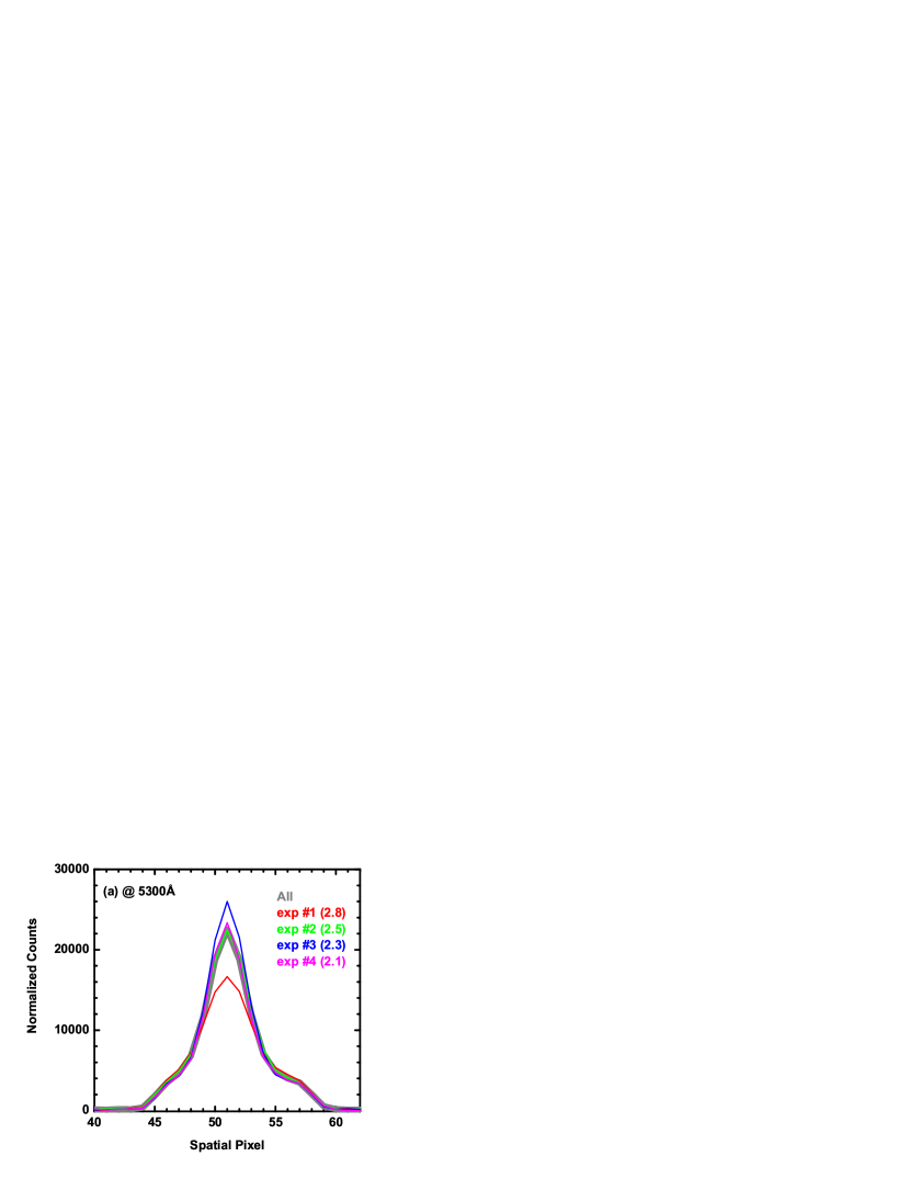
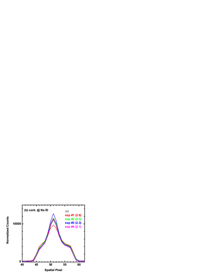
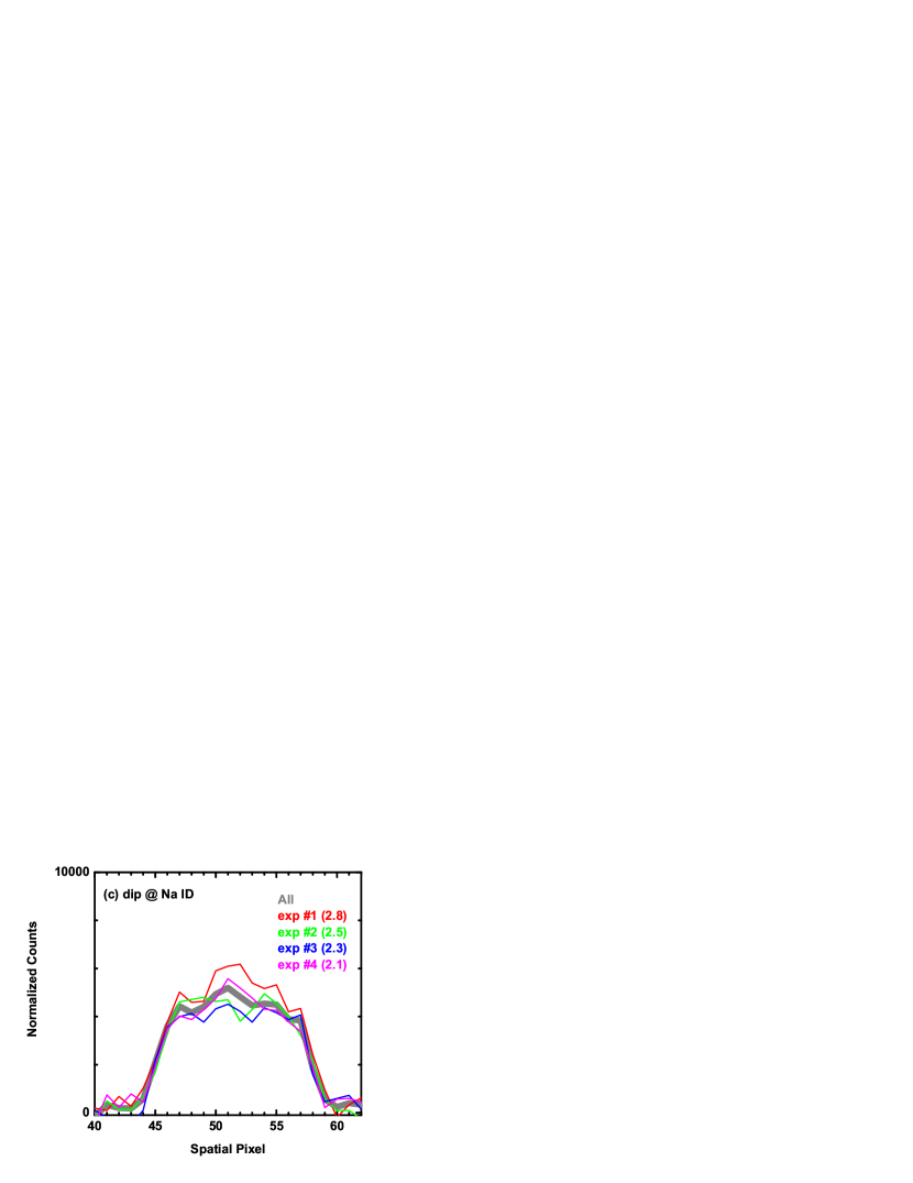
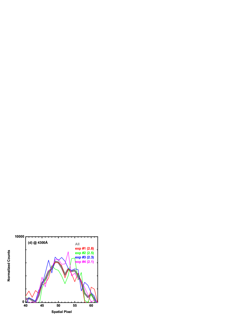
Figure 15.— (Figure A1): Spatial profiles of each individual exposure of the $+255.1$ day SN 2014J spectrum for different wavelength regions: (a) at $\sim$5300 Å, (b) a continuum around Na I D, (c) a dip at Na I D, and (d) at $\sim$4300 Å. In each panel, the spatial profile extracted from the combined 2D spectrum is shown in gray, while the profiles extracted from individual exposures are shown in other colors. The airmass for each exposure is shown in parentheses in the labels.

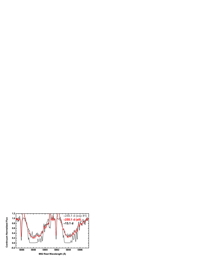
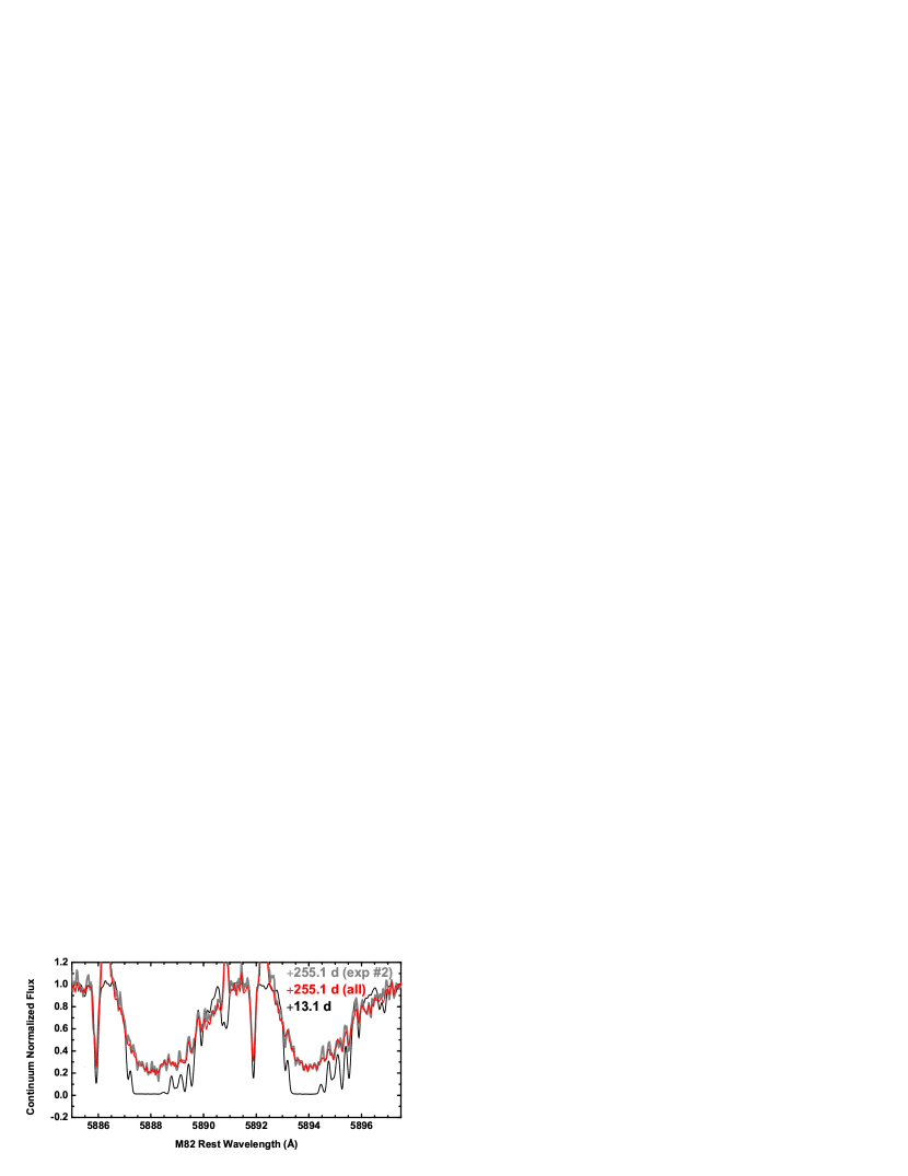
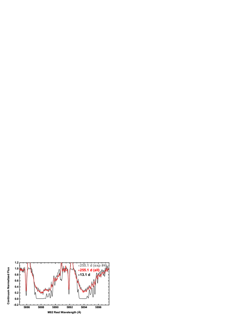
Figure 16.— (Figure A2): The $+255.1$ day spectrum of SN 2014J without subtracting the diffuse light, shown for each individual exposure (gray). For comparison, the spectrum extracted from the combined 2D spectrum is shown in red, as well as the $+13.1$ day spectrum in black.

Our observation at $+255.1$ days was performed at high airmass, ranging from $\sim$2.8 in the first exposure to $\sim$2.1 in the fourth exposure. As such, we want to test whether this high airmass and its evolution as a function of time could result in an unusually large seeing and/or temporal variability of FWHM depending on the airmass to a level that could affect our conclusions.

As shown in Figure 4, a point source (i.e., the SN) was clearly detected with FWHM of $\sim$0.8″. Figure A1 shows the spatial profiles of the incoming light extracted from the individual 2D images for each exposure. Indeed, there is a slight evolution in the FWHM of the point source component – it was $\sim$1″ in the first exposure but stayed at $\sim$0.8″ in the remaining exposures. Nevertheless, the line profiles at different wavelengths are consistent between different exposures, and the change in the seeing is too small to affect the observational features discussed in the main text.

Figures A2 and A3 show the continuum-normalized total light (A2) and DC-subtracted (A3) spectra of SN 2014J at $+255.1$ days. These are the same as in Figures 5 and 8, respectively, but extracted separately for each exposure. The individual exposures are consistent with each other and with the spectrum from the combined 2D image. From these analyses, we conclude that the high airmass did not affect any of our conclusions.

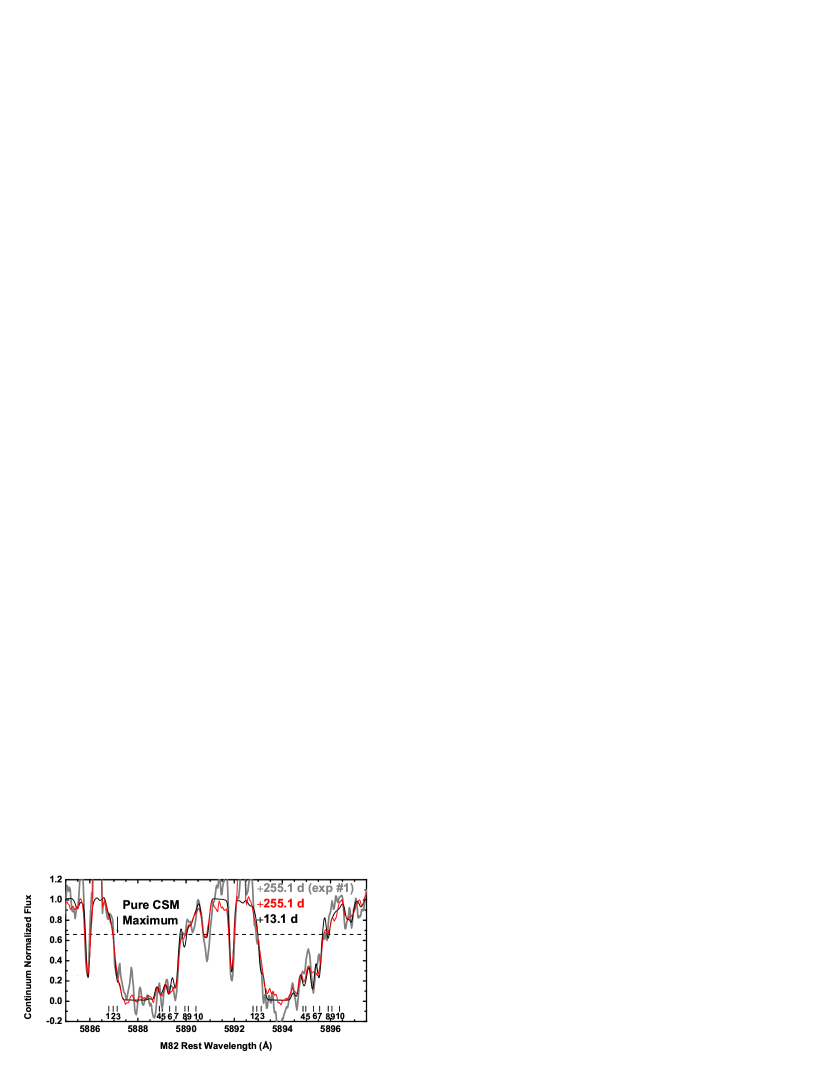
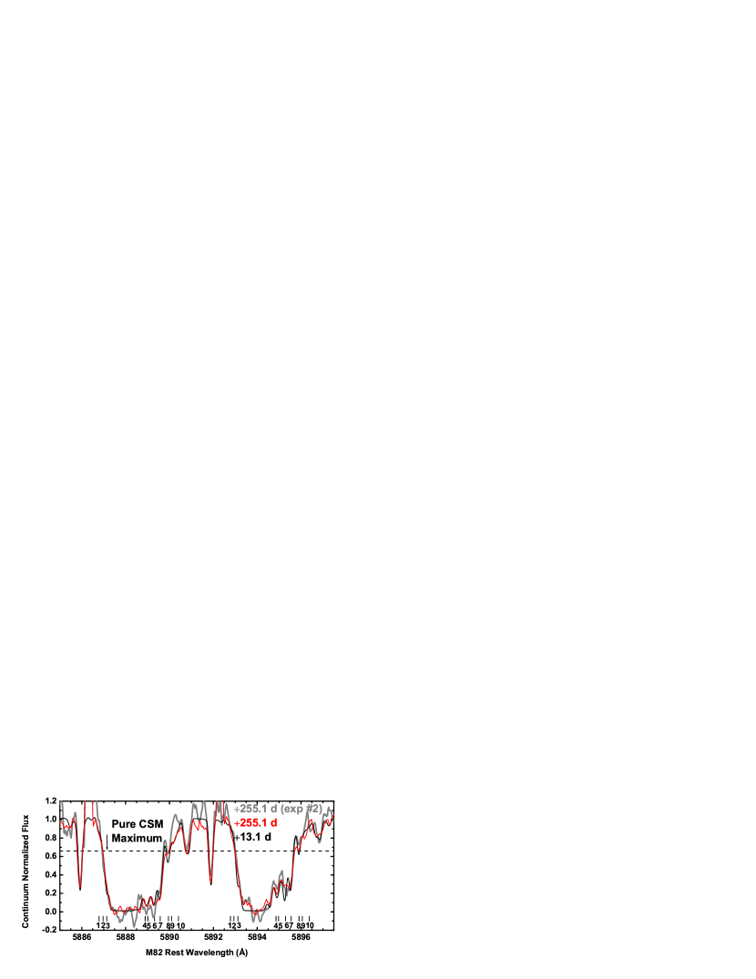
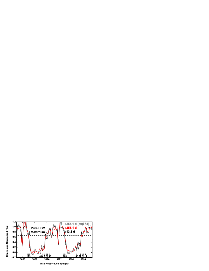
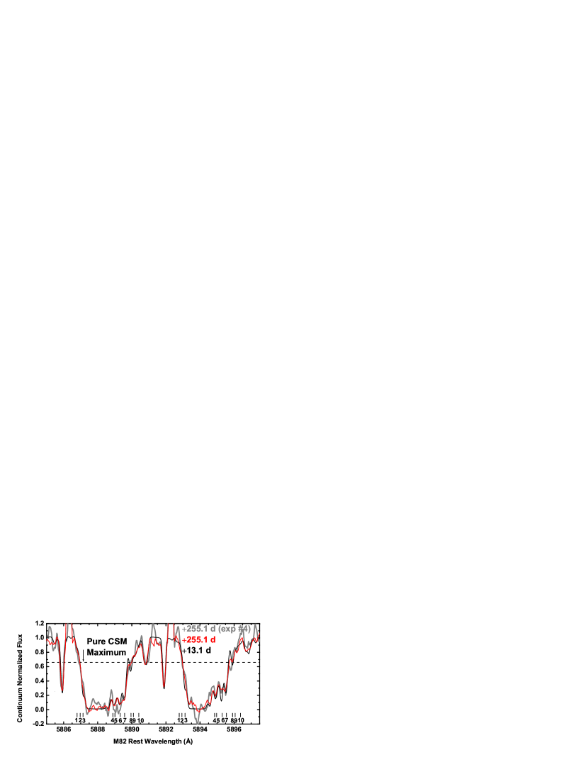
Figure 17.— (Figure A3): Spectrum of SN 2014J at $+255.1$ days relative to $B$-band maximum brightness with the subtraction of the contaminating diffuse component (DC model 1), shown for each individual exposure (gray, smoothed with a 7 pixel boxcar filter). For comparison, the spectrum extracted from the combined 2D spectrum is shown in red (also smoothed with a 7 pixel boxcar filter), as well as the $+13.1$ day spectrum in black.

Appendix B Analyses of the K I Feature

In this section, we provide a comparison between our $+45.1$ day spectrum and those from the APF (Graham et al., 2015), specifically using their earliest spectrum taken on $-11$ days and the last one taken on $+22$ days. To directly compare our spectrum taken by the Subaru telescope with the APF spectra, it is necessary to deal with a fringe pattern seen in the APF spectra. In doing this, we make one assumption – global patterns of the absorption line spectra are identical at $+22$ and $+45.1$ days, while allowing the narrow components at the scale of $\mathrel{\hbox to0.0pt{\lower 4.0pt\hbox{\hskip 1.0pt$\sim$}\hss}\raise 1.0pt\hbox{$<$}}$1 Å to vary as a function of time. This is possible since the fringing pattern has a characteristic size of $\mathrel{\hbox to0.0pt{\lower 4.0pt\hbox{\hskip 1.0pt$\sim$}\hss}\raise 1.0pt\hbox{$>$}}$1 Å while the real absorption is at a scale of $\mathrel{\hbox to0.0pt{\lower 4.0pt\hbox{\hskip 1.0pt$\sim$}\hss}\raise 1.0pt\hbox{$<$}}$1 Å.

First, the APF spectra are convolved with a Gaussian kernel so that the spectral resolution is degraded to match the Subaru resolution. Next, the APF spectrum on $+22$ days was divided by the Subaru spectrum on $+45.1$ days, resulting in a ‘fringe pattern function.’ We smoothed this function with a boxcar filter with a width of $\sim$1 Å. The result is used as the fringe pattern, and the APF spectrum of the same epoch was divided by this pattern. The result is a fringe-corrected spectrum as shown in Figure 12 (blue). While this assumes that the global pattern did not evolve, if there is a difference between the two spectra used to generate the fringe pattern (at $+22$ and $+45.1$ days) at a level narrower than $\sim$1 Å, one should be able to detect such features. The same procedure was performed for the APF spectrum on $-11$ days (gray) where the same APF spectrum ($-11$ days) was used to create the fringe pattern. As an additional cross check, we adopted the fringing pattern created with the APF spectrum on $+22$ days, then corrected the wavelength for the difference in the heliocentric velocities on $-11$ and $+22$ days, and finally subtracted this pattern from the spectrum on $-11$ days (black). Except for the slight change in the depth of features, which we attribute to differences in setting the continuum, these two versions of ‘fringe-free’ $-11$ day spectra are consistent. This supports the view that the method of subtracting the fringe pattern is robust.

The direct comparison between the Subaru spectrum and the APF spectra confirms the main conclusions reached by Graham et al. (2015). We do see the decreasing depths of the K I components at $-144$ km s^-1 and at $-127$ km s^-1 from $-11$ days to $+22$ days (after correcting for the fringing pattern using the new Subaru spectrum), while there are no significant changes in the other K I components. Comparing the APF and Subaru spectra, we see no significant evolution from $+20$ days to $+45.1$ days in the SN 2014J K I absorption profile.

References

- Amanullah et al. (2014) Amanullah, R., et al. 2014, ApJ, 788, L21
- Amanullah et al. (2015) Amanullah, R., et al. 2015, MNRAS, 453, 3300
- Ashall et al. (2014) Ashall, C., et al. 2014, MNRAS, 445, 4424
- Brown et al. (2015) Brown, P.J., et al. 2015, ApJ, 805, 74
- Cao et al. (2015) Cao, Y., et al. 2015, Nature, 521, 328
- Churazov et al. (2014) Churazov, E., et al. 2014, Nature, 512, 406
- Cox & Patat (2008) Cox, N.L.J., Patat, F. 2008, A&A, 485, L9
- Crotts (2015) Crotts, A.P.S. 2015, ApJ, 804, L37
- Diehl et al. (2014) Diehl, R, et al. 2014, Science, 345, 1162
- Foley et al. (2012) Foley, R.J., et al. 2012, ApJ, 752, 101
- Foley et al. (2014) Foley, R.J., et al. 2014, MNRAS, 443, 2887
- Fossey et al. (2014) Fossey, S., Cooke, B., Pollack, G., Wilde, M., Wright, T. 2014, CBET, 3792, 1
- Gao et al. (2015) Gao, J., Jiang, B.W., Li, A., Li, J,m Wang, X. 2015, ApJ, 807, L26
- Goobar (2008) Goobar, A., 2008, ApJ, 68, L103
- Goobar et al. (2014) Goobar, A., et al. 2014, ApJ, 784, L12
- Graham et al. (2015) Graham, M.L., et al. 2015, ApJ, 801, 136
- Hachisu et al. (1999) Hachisu, I., Kato, M., Nomoto, K. 1999, ApJ, 522, 487
- Hoang (2015) Hoang, T. 2015, arXiv:1510.01822
- Hillebrandt & Niemeyer (2000) Hillebrandt, W. & Niemeyer, J.C. 2000, ARA&A, 38, 191
- Iben & Tutukov (1984) Iben, Jr., I., Tutukov, A.V. 1984, ApJ, 284, 719
- Jack et al. (2015) Jack, D., et al. 2015, MNRAS, 451, 4104
- Johansson et al. (2014) Johansson, J., et al. 2014, arXiv:1411.3332
- Kambe et al. (2013) Kambe, E., et al. 2013, PASJ, 65, 15
- Kasen (2010) Kasen, D. 2010, ApJ, 708, 1025
- Kawabata et al. (2014) Kawabata, K.S., et al. 2014, ApJ, 795, L4
- Kutsuna & Shigeyama (2015) Kutsuna, M, Shigeyama, T. 2015, PASJ, 67, 54
- Kelly et al. (2014) Kelly, P.L., et al. 2014, ApJ, 790, 3
- Lundqvist et al. (2015) Lundqvist, P., et al. 2015, A&A, 577, A39
- Maeda et al. (2015) Maeda, K., Nozawa, T., Nagao, T., Motohara, K. 2015, MNRAS, 452, 3281
- Maguire et al. (2013) Maguire, K., et al. 2013, MNRAS, 436, 222
- Maoz et al. (2014) Maoz, D., Mannucci, F., Nelemans, G. 2014, ARA&A, 52, 107
- Margutti et al. (2014) Margutti, R., et al. 2014, ApJ, 790, 52
- Marion et al. (2015a) Marion, G.H., et al. 2015a, ApJ, 798, 39
- Marion et al. (2015b) Marion, G.H., et al. 2015b, arXiv:1507.07261
- Mayya & Carrasco (2009) Mayya, Y.D., Carrasco, L. 2009, RMxAC, 37, 44
- Milisavljevic et al. (2014) Milisavljevic, D., et al. 2014, ApJ, 782, L5
- Nielsen et al. (2014) Nielsen, M.T.B., Gilfanov, M., Bogdán, Á., Woods, T.E., Nelemans, G. 2014, MNRAS, 442, 3400
- Noguchi et al. (2002) Noguchi, K., et al. 2002, PASJ, 54, 855
- Nomoto (1982) Nomoto, K. 1982, ApJ, 253, 798
- Oke (1990) Oke, J. B. 1990, AJ, 99, 1621
- Patat et al. (2007) Patat, F., et al. 2007, Science, 317, 924
- Patat et al. (2015) Patat, F., et al. 2015, A&A, 577, 53
- Pérez-Torres et al. (2014) Pérez-Torres, M.A., et al. 2014, ApJ, 792, 38
- Raskin & Kasen (2013) Raskin, C., Kasen, D. 2013, ApJ, 772, 1
- Phillips et al. (2013) Phillips, M.M., et al. 2013, ApJ, 779, 38
- Rich (1987) Rich, R.M. 1987, AJ, 94, 651
- Ritchey et al. (2015) Ritchey, A.M., Welty, D.E., Dahlstrom, J.A., York, D.G. 2015, ApJ, 799, 197
- Shen et al. (2013) Shen, K.J., Guillochon, J., Folay, R.J. 2013, ApJ, 770, L35
- Simon et al. (2009) Simon, J.D., et al. 2009, ApJ, 702, 1157
- Soker (2015) Soker, N. 2015, MNRAS, 450, 1333
- Sparks & Stecher (1974) Sparks, W. M., Stecher, T. P. 1974, ApJ, 188, 149
- Stanishev et al. (2007) Stanishev, V., et al. 2007, A&A, 469, 645
- Sternberg et al. (2011) Sternberg, A., et al. 2011, Science, 333, 856
- Sternberg et al. (2014) Sternberg, A., et al. 2014, MNRAS, 443, 1849
- Tanikawa et al. (2015) Tanikawa, A., Nakasato, N., Sato, Y., Nomoto, K., Maeda, K., Hachisu, I. 2015, ApJ, 807, 40
- Telesco et al. (2015) Telesco, C.M., et al. 2015, ApJ, 798, 93
- Vacca et al. (2015) Vacca, W.D., et al. 2015, ApJ, 804, 66
- van Loon et al. (2009) van Loon, J. Th., Smith, K. T., McDonald, I. et al. 2009, MNRAS, 399, 195
- van Loon et al. (2013) van Loon, J. Th., Bailey, M., Tatton, B. L. et al. 2013, A&A, 550, 108
- Webbink (1984) Webbink, R.F. 1984, ApJ, 277, 355
- Welty et al. (2014) Welty, D.E., Ritchey, A.M., Dahlstrom, J.A., York, D.G. 2014, ApJ, 792, 106
- Whelan & Iben (1973) Whelan, J., Iben, Jr., I. 1973, ApJ, 186, 1007
- Zheng et al. (2014) Zheng, W., et al. 2014, ApJ, 783, L24