Constructive stability and stabilizability of positive linear discrete-time switching systems

Abstract

We describe a new class of positive linear discrete-time switching systems for which the problems of stability or stabilizability can be resolved constructively. The systems constituting this class can be treated as a natural generalization of systems with the so-called independently switching state vector components. Distinctive feature of such systems is that their components can be arbitrarily ‘re-connected’ in parallel or in series without loss of the ‘constructive resolvability’ property for the problems of stability or stabilizability of a system. It is shown also that, for such systems, the individual positive trajectories with the greatest or the lowest rate of convergence to the zero can be built constructively.

1 Introduction

A linear discrete-time system

$$x(n+1)=A(n)x(n),\quad x(n)\in\mathbb{R}^{N},$$ (1)

is called switching provided that the $(N\times N)$-matrices $A(n)$, for each $n$, may arbitrarily take values from some set $\mathscr{A}$. System (1) is called (asymptotically) stable if, for each sequence of matrices $A(n)\in\mathscr{A}$, $n=0,1,\ldots$, the corresponding solution $x(n)$ tends to zero. The asymptotic stability of switching system (1) is equivalent to the exponential convergence to zero of each sequence $\{X(n)\}$ of the matrix products $X(n)=A(n)\cdots A(1)A(0)$ [1, 2, 3, 4, 5, 6, 7, 8], which in turn is equivalent to the inequality

$$\rho(\mathscr{A})<1.$$ (2)

Here, the quantity $\rho(\mathscr{A})$, called [9] the joint spectral radius of the matrix set $\mathscr{A}$, is defined as follows:

$$\rho(\mathscr{A})=\lim_{n\to\infty}\sup\left\{\|A_{n}\cdots A_{1}\|^{1/n}:\leavevmode\nobreak\ A_{i}\in\mathscr{A}\right\},$$ (3)

where $\|\cdot\|$ is an arbitrary norm on $\mathbb{R}^{N\times N}$.

For switching systems that are not stable, one may pose the question about the existence of at least one sequence of matrices $A(n)\in\mathscr{A}$, $n=0,1,\ldots$, such that $A(n)\cdots A(1)A(0)\to 0$, that is, about stabilization of a system. It is known [4, 10, 11, 12, 13] that system (1) can be stabilized if the following inequality holds:

$$\check{\rho}(\mathscr{A})<1,$$ (4)

where the quantity $\check{\rho}(\mathscr{A})$, called the lower spectral radius [4] of the matrix set $\mathscr{A}$, is as follows:

$$\check{\rho}(\mathscr{A})=\lim_{n\to\infty}\inf\left\{\|A_{n}\cdots A_{1}\|^{1/n}:\leavevmode\nobreak\ A_{i}\in\mathscr{A}\right\}.$$ (5)

Inequalities (2) and (4) might seem to give an exhaustive answer to the questions on stability or stabilizability of a switching system. This is indeed the case from the theoretical point of view. However, in practice it is rather difficult, if at all possible, to calculate in a closed formula form the limits in (3) and (5), see, e.g., numerous negative results in [14, 15, 16, 17, 18, 19]. This implies the need to make use of approximate computational methods. Besides, currently there are no a priory estimates for the rate of convergence of the limits (3) and (5), and the required amount of computations rapidly increases in $n$ and the dimension of the system, which exacerbates the difficulty in the usage of computational methods. In this regard, we would like to note the following problems of stability and stabilizability of linear switching systems, which are not new per se, but remain to be relevant.

In this regard, we would like to note the following problems of stability and stabilizability of linear switching systems, which are not new per se, but remain to be relevant.

Problem 1.

How to describe the classes of switching systems (or equivalently, the classes of matrix sets $\mathscr{A}$), for which the joint spectral radius (3) could be constructively calculated?

Problem 2.

How to describe the classes of switching systems (or equivalently, the classes of matrix sets $\mathscr{A}$), for which the lower spectral radius (5) could be constructively calculated?

There is another circumstance that hampers the investigation of stability and stabilizability of system (1). This circumstance is barely mentioned in the theory of convergence of matrix products but is of crucial importance in control theory. The point is that, in control theory, systems in general are composed not of a single block but of a number of interconnected blocks. When these blocks are linear and functioning asynchronously each of them is described by the equation

$$x_{\text{out}}(n+1)=A_{i}(n)x_{\text{in}}(n),$$ (6)

where $x_{\text{in}}(\cdot)\in\mathbb{R}^{N_{i}}$, $x_{\text{out}}(\cdot)\in\mathbb{R}^{M_{i}}$, and the matrices $A_{i}(n)$, for each $n$, may arbitrarily take values from some set $\mathscr{A}_{i}$ of $(N_{i}\times M_{i})$-matrices, where $i=1,2,\ldots,Q$ and $Q$ is the total amount of blocks in the system.

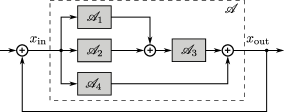
Figure 1: An example of a series-parallel connection of controllers of a system

In this case it is natural to pose the question about stability or stabilizability not for isolated blocks or controllers (6), but for the system as a whole, whose blocks may be connected in parallel or in series, or in a more complicated way, represented by some directed graph with blocks of the form (6) placed on its edges, see Fig. 1. Unfortunately, under such a connection of blocks, the classes of matrices describing the transient processes of a system as a whole became very complicated and their properties are practically not investigated. As a rule, even in the cases when the dimensions of the input-output vectors coincide with each other and hence the question about stability or stabilizability of a single block may be somehow answered, after a series-parallel connection of such blocks, it is often impossible to constructively resolve the question about the stability of the whole system or, at the best, it is very difficult to get the desired answer. So, the following problem is also urgent:

Problem 3.

How to describe the classes of switching systems for which the question about stability or stabilizability can be constructively answered not only for an isolated switching block (1) or (6) but also for any series-parallel connection of such blocks?

At last, let us consider one more aspect of the problem of constructive stability or stabilizability of the switching systems.

The joint spectral radius (3), as well as the lower spectral radius (5), provide only characterization of stability or stabilizability of a system ‘as a whole’. They describe the limiting behavior of the ‘multiplicatively averaged’ norms of the matrix products, $\|A(n-1)\cdots A(0)\|^{1/n}$. If one is interested in the study of stability of a system, in typical situations, e.g. for the so-called irreducible classes of matrices $\mathscr{A}$, for each sequence of matrices $\{A(n)\}$ the following estimate holds

$$\|A(n-1)\cdots A(0)\|\leq C\rho^{n}(\mathscr{A}),$$

see, e.g., [2]. In the case when one is interested in the study of stabilizability of a system, in typical situations there exists a sequence of matrices $\{A(n)\}$ such that the following estimate is valid:

$$\|A(n-1)\cdots A(0)\|\leq\check{C}\check{\rho}^{n}(\mathscr{A}).$$

At the same time there is often a need to find a sequence of matrices that would ensure the slowest or fastest ‘decrease’ not of the norms of matrix products $\|A(n-1)\cdots A(0)\|$ but, for a given initial vector $x$, of the vectors $A(n-1)\cdots A(0)x$. More precisely, let us consider a real function $\nu(x)\equiv\nu(x_{1},x_{2},\ldots,x_{N})$ which is non-decreasing in each coordinate $x_{i}$ of the vector $x=(x_{1},x_{2},\ldots,x_{N})$ and defined for all $x_{1},x_{2},\ldots,x_{N}\geq 0$. Such a function will be called coordinate-wise monotone, while in the case when it is strictly increasing in each variable $x_{i}$ it will be called strictly coordinate-wise monotone. For example, each of the norms

$$\|x\|_{1}=\sum_{i}|x_{i}|,\quad\|x\|_{2}=\sqrt{\sum_{i}|x_{i}|^{2}},\quad\|x\|_{\infty}=\max_{i}|x_{i}|,$$

is a coordinate-wise monotone function. Moreover, the norms $\|x\|_{1}$ and $\|x\|_{2}$ are strictly coordinate-wise monotone whereas the norm $\|x\|_{\infty}$ is coordinate-wise monotone but not strictly coordinate-wise monotone.

If a set of matrices $\mathscr{A}$ is finite and consists of $K$ elements then to find the value of

$$\max_{A\in\mathscr{A}}\nu(Ax)$$

it is needed, in general, to compute $K$ times the values of the function $\nu(\cdot)$, and then to find their maximum. Similarly, to find the value of

$$\max_{A_{i_{j}}\in\mathscr{A}}\nu(A_{i_{n}}\cdots A_{i_{1}}x)$$ (7)

one need, in general, to compute $K^{n}$ times the values of the function $\nu(\cdot)$, and then to find their maximum, which leads to an exponential in $n$ growth of the number of required computations. Therefore, it is reasonable to put the following problem:

Problem 4.

Given a coordinate-wise monotone function $\nu(\cdot)$ and a vector $x\neq 0$. How to describe the classes of switching systems (or equivalently, the classes of matrix sets $\mathscr{A}$), for which the number of computations of the function $\nu(\cdot)$ needed to find the quantity (7) would be less than $K^{n}$? It is desirable that the required number of computations would be of order $Kn$.

Clearly, a similar problem about minimization of the quantity $\nu(A_{i_{n}}\cdots A_{i_{1}}x)$ can also be posed.

In connection with this, our aim is to describe a class of asynchronous blocks or controllers (1), rather simple and natural in applications, for which one can obtain affordable answers to Problems 1–4.

In Section 2, we recall some facts from the theory of matrix products.

2 Sets of matrices with constructively computable spectral characteristics

One of classes of matrix sets whose characteristics (3) and (5) may be constructively calculated is the so-called class of positive matrix sets with independent row uncertainty [20]. Recall the related definitions.

In accordance with [20], a set of $N\times M$-matrices $\mathscr{A}$ is called a set with independent row uncertainty, or an IRU-set, if it consists of all the matrices

$$A=\begin{pmatrix}a_{11}&a_{12}&\cdots&a_{1M}\\ a_{21}&a_{22}&\cdots&a_{2M}\\ \cdots&\cdots&\cdots&\cdots\\ a_{N1}&a_{N2}&\cdots&a_{NM}\end{pmatrix},$$

each row $a_{i}=(a_{i1},a_{i2},\ldots,a_{iM})$ of which belongs to some set of rows $\mathscr{A}^{(i)}$, $i=1,2,\ldots,N$. An IRU-set of matrices will be referred to as positive if all its matrices are positive, which is equivalent to the positivity of all strings composing the sets $\mathscr{A}^{(i)}$. The totality of all IRU-sets of positive $(N\times M)$-matrices will be denoted by $\mathcal{U}(N,M)$.

Example 1.

Let the sets of rows $\mathscr{A}^{(1)}$ and $\mathscr{A}^{(2)}$ be as follows:

$$\mathscr{A}^{(1)}=\{(a,b),\leavevmode\nobreak\ (c,d)\},\leavevmode\nobreak\ \mathscr{A}^{(2)}=\{(\alpha,\beta),\leavevmode\nobreak\ (\gamma,\delta),\leavevmode\nobreak\ (\mu,\nu)\}.$$

Then the IRU-set $\mathscr{A}$ consists of the following matrices:

$$A_{11} =\begin{pmatrix}a&b\\ \alpha&\beta\end{pmatrix}, \leavevmode\nobreak\ A_{12} =\begin{pmatrix}a&b\\ \gamma&\delta\end{pmatrix}, \leavevmode\nobreak\ A_{13} =\begin{pmatrix}a&b\\ \mu&\nu\end{pmatrix},$$

$$A_{21} =\begin{pmatrix}c&d\\ \alpha&\beta\end{pmatrix}, \leavevmode\nobreak\ A_{22} =\begin{pmatrix}c&d\\ \gamma&\delta\end{pmatrix}, \leavevmode\nobreak\ A_{23} =\begin{pmatrix}c&d\\ \mu&\nu\end{pmatrix}.$$

If a set $\mathscr{A}$ is compact, which is equivalent to the compactness of each set of rows $\mathscr{A}^{(1)}$, $\mathscr{A}^{(2)}$, …, $\mathscr{A}^{(N)}$, then the following quantities are well defined:

$$\rho_{min}(\mathscr{A})=\min_{A\in\mathscr{A}}\rho(A),\quad\rho_{max}(\mathscr{A})=\max_{A\in\mathscr{A}}\rho(A).$$

As is shown in [21, 22],

$$\rho(\mathscr{A})=\rho_{max}(\mathscr{A}),\quad\check{\rho}(\mathscr{A})=\rho_{min}(\mathscr{A}),$$ (8)

for positive compact IRU-sets of matrices $\mathscr{A}$, whereas for arbitrary sets of matrices the equalities in (8) are not valid, see [22, Example 1].

For finite IRU-sets of matrices $\mathscr{A}$, the quantities $\rho_{min}(\mathscr{A})$ and $\rho_{max}(\mathscr{A})$ can be constructively calculated, and therefore due to (8), for finite IRU-sets of positive matrices, the quantities $\rho(\mathscr{A})$ and $\check{\rho}(\mathscr{A})$ are also can be constructively calculated. An efficient computational algorithm for finding the quantities $\rho_{min}(\mathscr{A})$ and $\rho_{max}(\mathscr{A})$, for various IRU-sets of matrices $\mathscr{A}$, is proposed in [23].

Another example of classes of matrices, for which the quantities (3) and (5) can be constructively calculated, is given by the so-called linearly ordered sets of positive matrices $\mathscr{A}=\{A_{1},A_{2},\ldots,A_{n}\}$, that is, such sets of matrices for which $0<A_{1}<A_{2}<\cdots<A_{n}$, where the inequalities are meant element-wise. For this class of matrices, equalities (8) follow from the known relations between the spectral radii of comparable positive matrices [24, Corollary 8.1.19]. The totality of all linearly ordered sets of $(N\times M)$-matrices will be denoted by $\mathcal{L}(N,M)$.

It should be noted that controllers or blocks whose behavior is covered by equations (1) or (6) with IRU-sets of matrices are rather common asynchronous controllers in control theory which perform the so-called independent coordinate-wise correction of the state vectors. The controllers whose whose behavior is covered by equations (1) or (6) with linearly ordered sets of matrices are a kind of amplifiers with ‘matrix’ coefficients of amplification varying in time.

In [22] it was observed that the proofs of equalities (8) for the IRU-sets of positive matrices, as well as for the linearly ordered sets of positive matrices, may be obtained by the same scheme, as a corollary of some general principle, which we now describe in more detail.

2.1 Hourglass alternative

For vectors $x,y\in\mathbb{R}^{N}$, we write $x\geq y$ ($x>y$), if all coordinates of the vector $x$ are not less (strictly greater), than the corresponding coordinates of the vector $y$. Similar notation will be applied to matrices.

A set of positive matrices $\mathscr{A}$ is called an $\mathcal{H}$-set [22] if, for any matrix $\tilde{A}\in\mathscr{A}$ and any vector $x>0$, the following assertions hold:

1. either $Ax\geq\tilde{A}x$ for all $A\in\mathscr{A}$ or there exists a matrix $\bar{A}\in\mathscr{A}$ such that $\bar{A}x\leq\tilde{A}x$ and $\bar{A}x\neq\tilde{A}x$;

2. either $Ax\leq\tilde{A}x$ for all $A\in\mathscr{A}$ or there exists a matrix $\bar{A}\in\mathscr{A}$ such that $\bar{A}x\geq\tilde{A}x$ and $\bar{A}x\neq\tilde{A}x$.

Assertions H1 and H2 have a simple geometrical interpretation. Imagine that the sets $\{u:u\leq\tilde{A}x\}$ and $\{u:u\geq\tilde{A}x\}$ form the lower and upper bulbs of some stylized hourglass with the neck at the point $\tilde{A}x$. Then, according to Assertions H1 and H2, either all the ‘grains’ $Ax$ fill one of the bulbs (upper or lower), or at least one grain remains in the other bulb (lower or upper, respectively). In [22], such an interpretation gave reason to call Assertions H1 and H2 the hourglass alternative.

The totality of all compact $\mathcal{H}$-sets of matrices of dimension $N\times M$ will be denoted by $\mathcal{H}(N,M)$. Then the main result about the spectral properties of the $\mathcal{H}$-sets of matrices can be formulated as follows.

Theorem 1 (see [22]).

Let $\mathscr{A}\in\mathcal{H}(N,N)$. Then equalities (8) hold.

As a matter of fact, in [22] a number of more profound results are proved, but we will not delve into the intricacies.

2.2 $\mathcal{H}$-sets of matrices

The applicability of Theorem 1 essentially depends on how constructive one will be able to describe the classes of $\mathcal{H}$-sets of matrices. In [22] it was shown that the sets of matrices with independent row uncertainty and the linearly ordered sets of positive matrices are $\mathcal{H}$-sets of matrices. However, as demonstrates Example 2 below, not every set of positive matrices is an $\mathcal{H}$-set. The one-element sets of matrices $\{0\}$ and $\{I\}$ consisting of the zero and the identity matrices are also not $\mathcal{H}$-sets because the related matrices are not positive.

Example 2.

Let us consider the set of matrices $\mathscr{A}=\{A_{1},A_{2}\}$, where

$$A_{1}=\begin{pmatrix}a&a^{2}\\ 1&a\hphantom{\leavevmode\nobreak\ }\end{pmatrix},\quad A_{2}=\begin{pmatrix}a\hphantom{\leavevmode\nobreak\ }&1\\ a^{2}&a\end{pmatrix},\qquad a>0.$$

Then $\max\{\rho(A_{1}),\rho(A_{2})\}=2a$ and $\rho(A_{1}A_{2})=(1+a^{2})^{2}$. Therefore, for $a\neq 1$,

$$\rho(\mathscr{A})\geq\|A_{1}A_{2}\|^{1/2}\geq\rho(A_{1}A_{2})^{1/2}>\max\{\rho(A_{1}),\rho(A_{2})\},$$

which by Theorem 1 could not be valid if $\mathscr{A}$ was an $\mathcal{H}$-set of matrices.

To construct other classes of $\mathcal{H}$-sets of matrices let us ascertain some general properties of such sets of matrices. Introduce the operations of Minkowski addition and multiplication for sets of matrices:

$$\mathscr{A}+\mathscr{B} :=\{A+B:A\in\mathscr{A},\leavevmode\nobreak\ B\in\mathscr{B}\},$$

$$\mathscr{A}\mathscr{B} :=\{AB:A\in\mathscr{A},\leavevmode\nobreak\ B\in\mathscr{B}\},$$

and also the operation of multiplication of a set of matrices by a number:

$$t\mathscr{A}=\mathscr{A}t:=\{tA:t\in\mathbb{R},\leavevmode\nobreak\ A\in\mathscr{A}\}.$$

The Minkowski addition of sets of matrices corresponds to the parallel coupling of two independently operating asynchronous controllers, while the Minkowski multiplication corresponds to the serial connection of such asynchronous controllers.

Remark 1.

In general, $\mathscr{A}(\mathscr{B}_{1}+\mathscr{B}_{2})\neq\mathscr{A}\mathscr{B}_{1}+\mathscr{A}\mathscr{B}_{2}$ and $(\mathscr{A}_{1}+\mathscr{A}_{2})\mathscr{B}\neq\mathscr{A}_{1}\mathscr{B}+\mathscr{A}_{2}\mathscr{B}$, i.e. the Minkowski operations are not associative. In particular, $\mathscr{A}+\mathscr{A}\neq 2\mathscr{A}$.

Clearly, the operation of addition is admissible if the matrices from the set $\mathscr{A}$ are of the same size as the matrices from the set $\mathscr{B}$ , while the operation of multiplication is admissible if the sizes of the matrices from sets $\mathscr{A}$ and $\mathscr{B}$ are matched: the dimension of the rows of the matrices from $\mathscr{A}$ is the same as the dimension of the columns of the matrices from $\mathscr{B}$. There is no problem with matching of sizes when one considers sets of square matrices of the same size.

Theorem 2 (see [22]).

The following is true:

1. $\mathscr{A}+\mathscr{B}\in\mathcal{H}(N,M)$, if $\mathscr{A},\mathscr{B}\in\mathcal{H}(N,M)$;

2. $\mathscr{A}\mathscr{B}\in\mathcal{H}(N,Q)$, if $\mathscr{A}\in\mathcal{H}(N,M)$ and $\mathscr{B}\in\mathcal{H}(M,Q)$;

3. $t\mathscr{A}=\mathscr{A}t\in\mathcal{H}(N,M)$, if $t>0$ and $\mathscr{A}\in\mathcal{H}(N,M)$.

By Theorem 2 the totality of sets of square matrices $\mathcal{H}(N,N)$ is endowed with additive and multiplicative binary operations, but itself is not a group, neither additive nor multiplicative. However, after adding the zero additive element $\{0\}$ and the identity multiplicative element $\{I\}$ to $\mathcal{H}(N,N)$, the resulting totality $\mathcal{H}(N,N)\cup\{0\}\cup\{I\}$ becomes a semiring [25].

The fact that the totality $\mathcal{H}(N,N)$ is endowed with the operations of addition and multiplication means that, by connecting in a serial-parallel manner independently operating asynchronous controllers that satisfy the axioms H1 and H2, we again obtain an asynchronous controller satisfying the axioms H1 and H2.

Remark 2.

Theorem 2 implies that any finite sum of any finite products of sets of matrices from $\mathcal{H}(N,N)$ is again a set of matrices from $\mathcal{H}(N,N)$. Moreover, for any integers $n,d\geq 1$, all the polynomial sets of matrices

$$P(\mathscr{A}_{1},\mathscr{A}_{2},\ldots,\mathscr{A}_{n})=\sum_{k=1}^{d}\sum_{i_{1},i_{2},\ldots,i_{k}\in\{1,2,\ldots,n\}}p_{i_{1},i_{2},\ldots,i_{k}}\mathscr{A}_{i_{1}}\mathscr{A}_{i_{2}}\cdots\mathscr{A}_{i_{k}},$$ (9)

where $\mathscr{A}_{1},\mathscr{A}_{2},\ldots,\mathscr{A}_{n}\in\mathcal{H}(N,N)$ and the scalar coefficients $p_{i_{1},i_{2},\ldots,i_{k}}$ are positive, belong to the set $\mathcal{H}(N,N)$.

With the help of polynomials (9) one can construct not only the elements of the set $\mathcal{H}(N,N)$ but also the elements of arbitrary sets $\mathcal{H}(N,M)$, by taking the arguments $\mathscr{A}_{1},\mathscr{A}_{2},\ldots,\mathscr{A}_{n}$ from the sets $\mathcal{H}(N_{i},M_{i})$ with arbitrary matrix sizes $N_{i}\times M_{i}$. One must only ensure that the products $\mathscr{A}_{i_{1}}\mathscr{A}_{i_{2}}\cdots\mathscr{A}_{i_{k}}$ were admissible, and the expression (9) would determine the sets of matrices of dimension $N\times M$.

We have presented above two types of non-trivial $\mathcal{H}$-sets of matrices, the sets of positive matrices with independent row uncertainty and the linearly ordered sets of positive matrices. In this connection, let us denote by $\mathcal{H}_{*}(N,M)$ the totality of all sets of $(N\times M)$-matrices which can be obtained as the recursive expansion with the help of polynomials (9) of the sets of positive matrices with independent rows uncertainty and the sets of linearly ordered positive matrices. In other words, $\mathcal{H}_{*}(N,M)$ is the totality of all sets of matrices that can be represented as the values of superpositions of matrix polynomials (9) with the arguments of the polynomials of the ‘lowest level’ taken from the sets of the matrices belonging to $\mathcal{U}(N_{i},M_{i})\cup\mathcal{L}(N_{i},M_{i})$.

As was noted in Remark 1 the Minkowski operations are not associative. Therefore the recursive extension of the set of positive matrices with independent rows uncertainty and of linearly ordered positive matrices forms a wider variety of matrices than the extension of the set of positive matrices with independent rows uncertainty and of linearly ordered positive matrices with the help of polynomials (9).

3 Main result

Theorems 1 and 2, and Remark 2 imply the following statement:

Theorem 3.

Given a system (1) formed by a series-parallel recursive connection of blocks (6) (i.e. represented by some graph obtained by applying recursively series and/or parallel extensions starting form one edge, and with blocks placed on its edges) corresponding to some $\mathcal{H}$-sets of positive matrices $\mathscr{A}_{i}$, $i=1,2,\ldots,Q$. Then the question of the stability (stabilizability) of such a system can be constructively resolved by finding a matrix that maximizes (minimizes) the quantity $\rho(A)$ over the set of matrices $\mathscr{A}$, where $\mathscr{A}$ is the Minkowski polynomial sum (9) of the sets of matrices $\mathscr{A}_{i}$, $i=1,2,\ldots,Q$, corresponding to the structure of coupling of the related blocks.

Example 3.

For the system $\mathscr{A}$ in Fig. 1, the input and output are related by the equality

$$x_{\text{out}}(n+1)=\bigl{(}A_{3}(n)(A_{1}(n)+A_{2}(n))+A_{4}(n)\bigr{)}x_{\text{in}}(n),$$

where, for each $n$, the matrices $A_{1}(n),A_{2}(n),A_{3}(n)$ and $A_{4}(n)$ are randomly selected from the related sets: $A_{i}(n)\in\mathscr{A}_{i}$, $i=1,2,3,4$. Correspondingly, in this case all the possible values of the transition matrix for the system $\mathscr{A}$ can be obtained as the elements of the following Minkowski polynomial sum of the sets of matrices $\mathscr{A}_{1},\mathscr{A}_{2},\mathscr{A}_{3},\mathscr{A}_{4}$:

$$P(\mathscr{A}_{1},\mathscr{A}_{2},\mathscr{A}_{3},\mathscr{A}_{4})=\mathscr{A}_{3}(\mathscr{A}_{1}+\mathscr{A}_{2})+\mathscr{A}_{4}.$$

4 Construction of individual maximizing and minimizing sequences

4.1 One-step maximization

We first consider the problem of maximizing the function $\nu(Ax)$, where $x>0$, over all $A$ from the $\mathcal{H}$-set $\mathscr{A}$, which is assumed to be compact. By Assertion H2 of the hourglass alternative, for any matrix $\tilde{A}\in\mathscr{A}$, either $Ax\leq\tilde{A}x$ for all $A\in\mathscr{A}$ or there exists a matrix $\bar{A}\in\mathscr{A}$ such that $\bar{A}x\geq\tilde{A}x$ and $\bar{A}x\neq\tilde{A}x$. This together with the compactness of the set $\mathscr{A}$ implies the existence of a matrix $A^{(max)}\in\mathscr{A}$ such that, for all $A\in\mathscr{A}$, the following inequality holds:

$$Ax\leq A^{(max)}x.$$ (10)

Let us notice that the matrix $A^{(max)}$ depends on the vector $x$, and therefore, when needed, we will write $A^{(max)}=A^{(max)}_{x}$. Moreover, the matrix $A^{(max)}_{x}$ is generally determined non-uniquely by the vector $x$.

Theorem 4.

Let $\mathscr{A}$ be a compact $\mathcal{H}$-set of positive $(N\times N)$-matrices, $\nu(\cdot)$ be a coordinate-wise monotone function, and $x\in\mathbb{R}^{N}$, $x>0$, be a vector.

1. Then the maximum of the function $\nu(Ax)$ over $A\in\mathscr{A}$ is attained at the matrix $A^{(max)}=A^{(max)}_{x}$, that is,

   $$\max_{A\in\mathscr{A}}\nu(Ax)=\nu(A^{(max)}x).$$

2. If the maximum of the function $\nu(Ax)$ over $A\in\mathscr{A}$ is attained at a matrix $A_{0}\in\mathscr{A}$ and the function $\nu(\cdot)$ is strictly coordinate-wise monotone, then $A_{0}x=A^{(max)}_{x}x$.

Proof.

Assertion (i) directly follows from inequality (10) and the coordinate-wise monotonicity of the function $\nu(\cdot)$.

To prove Assertion (ii) let us notice that

$$A_{0}x\leq A^{(max)}_{x}x.$$

If here $A_{0}x\neq A^{(max)}_{x}x$ then at least one coordinate of the vector $A^{(max)}_{x}x$ should be strictly greater than the respective coordinate of the vector $A_{0}x$. Then, due to the strict coordinate-wise monotonicity of the function $\nu(\cdot)$, the following inequality holds:

$$\nu(A_{0}x)<\nu(A^{(max)}_{x}x),$$

which contradicts to the assumption that the maximum of the function $\nu(Ax)$ over $A\in\mathscr{A}$ is attained at the matrix $A_{0}\in\mathscr{A}$. Therefore, $A_{0}x=A^{(max)}_{x}x$, and Assertion (ii) is proved. ∎

Remark 3.

If the function $\nu(\cdot)$ is coordinate-wise monotone but not strictly coordinate-wise monotone then, in general, Assertion (ii) of Theorem 4 is not valid.

Remark 4.

The construction of the matrix $A^{(max)}$ does not depend on the function $\nu(\cdot)$.

4.2 Multi-step maximization: solution of Problem 4

We turn now to the question of determining the quantity (7) for some $n>1$ and $x\in\mathbb{R}^{N}$, $x>0$. With this aim in view, let us construct sequentially the matrices $A^{(max)}_{i}$, $i=1,2,\ldots,n$, as follows:

• the matrix $A^{(max)}_{1}$, depending in the vector $x_{0}=x$, is constructed in the same way as was done in the previous section: $A^{(max)}_{1}=A^{(max)}_{x_{0}}$;

• if the matrices $A^{(max)}_{i}$, $i=1,2,\ldots,k$, have already constructed then the matrix $A^{(max)}_{k+1}$, depending on the vector

  $$x_{k}=A^{(max)}_{k}\cdots A^{(max)}_{1}x,$$

  is constructed to maximize the function

  $$\nu(AA^{(max)}_{k}\cdots A^{(max)}_{1}x)=\nu(Ax_{k})$$

  over all $A\in\mathscr{A}$ in the same manner as was done in the previous section. So, the matrix $A^{(max)}_{k+1}$ is defined by the equality $A^{(max)}_{k+1}=A^{(max)}_{x_{k}}$.

By definition of the matrices $A^{(max)}_{i}$ then, in view of (10), for all $A\in\mathscr{A}$ the following inequalities hold:

$$Ax \leq A^{(max)}_{1}x,$$

$$AA^{(max)}_{1}x \leq A^{(max)}_{2}A^{(max)}_{1}x,$$

$$\ldots$$

$$AA^{(max)}_{n-1}\cdots A^{(max)}_{1}x \leq A^{(max)}_{n}\cdots A^{(max)}_{1}x,$$

which implies

$$A_{n}\cdots A_{1}x \leq A^{(max)}_{n}\cdots A^{(max)}_{1}x$$ (11)

for all $A_{n},\ldots,A_{1}\in\mathscr{A}$.

Theorem 5.

Let $\mathscr{A}$ be a compact $\mathcal{H}$-set of positive $(N\times N)$-matrices, $\nu(\cdot)$ be a coordinate-wise monotone function, and $x\in\mathbb{R}^{N}$, $x>0$, be a vector.

1. Then the maximum of the function $\nu(A_{n}\cdots A_{1}x)$ over $A_{1},\ldots,A_{n}\in\mathscr{A}$ is attained at the set of matrices $A^{(max)}_{1},\ldots,A^{(max)}_{n}$, that is,

   $$\max_{A_{n},\ldots,A_{1}\in\mathscr{A}}\nu(A_{n}\cdots A_{1}x)=\nu(A^{(max)}_{n}\cdots A^{(max)}_{1}x).$$

2. Let $\mathscr{A}$ be a compact $\mathcal{H}$-set of positive matrices. If the maximum of the function $\nu(A_{n}\cdots A_{1}x)$ over $A_{n},\ldots,A_{1}\in\mathscr{A}$ is attained at a set of matrices $\tilde{A}_{1},\ldots,\tilde{A}_{n}$ and the function $\nu(\cdot)$ is strictly coordinate-wise monotone, then

   $$\tilde{A}_{i}\cdots\tilde{A}_{1}x=A^{(max)}_{i}\cdots A^{(max)}_{1}x,\qquad i=1,2,\ldots,n.$$ (12)

Proof.

Assertion (i) directly follows from inequality (11) and the coordinate-wise monotonicity of the function $\nu(\cdot)$.

To prove Assertion (ii) let us observe that

$$\tilde{A}_{1}x \leq A^{(max)}_{1}x,$$

$$\tilde{A}_{2}\tilde{A}_{1}x \leq A^{(max)}_{2}A^{(max)}_{1}x,$$

$$\ldots$$

$$\tilde{A}_{n}\tilde{A}_{n-1}\cdots\tilde{A}_{1}x \leq A^{(max)}_{n}\cdots A^{(max)}_{1}x,$$

If here equalities (12) are not valid for some $i=i_{0}$ but valid for all $i<i_{0}$ then at least one coordinate of the vector $A^{(max)}_{i_{0}}\cdots A^{(max)}_{1}x$ is strictly greater than the respective coordinate of the vector $\tilde{A}_{i_{0}}\cdots\tilde{A}_{1}x$. Then, due to the positivity of the matrices from the set $\mathscr{A}$, for each $j\geq i_{0}$ there is valid the inequality

$$\tilde{A}_{j}\tilde{A}_{j-1}\cdots\tilde{A}_{1}x\leq A^{(max)}_{j}\cdots A^{(max)}_{1}x,$$

where at least one coordinate of the vector $A^{(max)}_{j}\cdots A^{(max)}_{1}x$ is strictly greater than the respective coordinate of the vector $\tilde{A}_{j}\tilde{A}_{j-1}\cdots\tilde{A}_{1}x$. Then, due to the strict coordinate-wise monotonicity of the function $\nu(\cdot)$, for $j=n$ we obtain the inequality

$$\nu(\tilde{A}_{n}\cdots\tilde{A}_{1}x)<\nu(A^{(max)}_{n}\cdots A^{(max)}_{1}x),$$

contradicting to the assumption that the maximum of the function $\nu(A_{n}\cdots A_{1}x)$ over $A_{n},\ldots,A_{1}\in\mathscr{A}$ is attained at the set of matrices $\tilde{A}_{1}\ldots,\tilde{A}_{n}$. Therefore, equalities (12) should be valid for all $i=1,2,\ldots,n$, and Assertion (ii) is proved. ∎

Remark 5.

The construction of each subsequent matrix $A^{(max)}_{i}$ is ‘positional’ or, what is the same, it is made in accordance with the ‘principles of dynamic programming’, that is, only based on the information known up to this step. At the same time, this construction does not depend on the function $\nu(\cdot)$, and hence on the complexity of its calculation!

5 Non-negative matrices

In the previous sections, all the considerations have been carried out for classes of matrices with positive elements. Sometimes, the requirement of positivity of the related matrices may be restrictive, however the transition to the matrices with arbitrary elements is hardly possible in the context of the treated problems, see [22] and the discussion therein. Even the transition to matrices with non-negative elements is not always possible, since in general, for such matrices, the constructions and statements of Section 2 are no longer valid. Nevertheless, in one particular case of practical interest the transition to non-negative matrices is possible.

Denote by $\overline{\mathcal{U}}(N,M)$ the totality of all IRU-sets of non-negative $(N\times M)$-matrices, and by $\overline{\mathcal{L}}(N,M)$ denote the totality of all sets $\mathscr{A}=\{A_{1},A_{2},\ldots,A_{n}\}$ of non-negative $(N\times M)$-matrices satisfying the inequalities $0\leq A_{1}\leq A_{2}\leq\cdots\leq A_{n}$. The totalities of sets of non-negative matrices $\overline{\mathcal{U}}(N,M)$ and $\overline{\mathcal{L}}(N,M)$ can be naturally treated as a kind of ‘closure’ of the related totalities of positive matrices $\mathcal{U}(N,M)$ and $\mathcal{L}(N,M)$.

Now, denote by $\overline{\mathcal{H}}_{*}(N,M)$ the totality of all sets of matrices that can be represented as the values of polynomials (9) with the arguments taken from the sets of matrices belonging to $\overline{\mathcal{U}}(N_{i},M_{i})\cup\overline{\mathcal{L}}(N_{i},M_{i})$. In this case, the totality $\overline{\mathcal{H}}_{*}(N,M)$ is no longer belongs to $\mathcal{H}(N,M)$ but, as was shown in [22], for each matrix $\mathscr{A}\in\overline{\mathcal{H}}_{*}(N,N)$ equalities (8) remain valid, i.e. an analog of Theorem 1 holds.

6 Conclusion

One of the most prominent problem in the design of control systems with switching components is that of evaluating (computing) the joint or lower spectral radii of the resulting system which determine its stability or stabilizability, respectively.

The approach to resolving this problem proposed in the article is fulfilled in compliance with the concept of modular design of control systems. It can be compared with the creation of toys with the help of a LEGO^® kit.

Recall that any LEGO^® kit consists of pieces (bricks and plates with stubs) arranging which in almost arbitrary order (oriented due to the presence of stubs) one can create a variety of structures.

Each $\mathcal{H}$-set of matrices $\mathscr{A}$ also can be interpreted as a kind of a LEGO^® kit for assembling control systems whose pieces (bricks and plates in a LEGO^® kit) are the switching blocks (controllers) with the transition characteristics determined by the matrix sets $\mathscr{A}_{i}\in\mathscr{A}$. Then, as was shown above, any series-parallel recursive connection of these blocks will result in creation of a system whose joint and lower spectral radii always can be computed constructively by formula (8).

References

- [1] A. F. Kleptsyn, V. S. Kozyakin, M. A. Krasnosel′skiĭ, N. A. Kuznetsov, Stability of desynchronized systems, Dokl. Akad. Nauk SSSR 274 (5) (1984) 1053–1056, in Russian, translation in Soviet Phys. Dokl. 29 (1984), 92–94.
- [2] N. E. Barabanov, On the Lyapunov exponent of discrete inclusions. I-III, Automat. Remote Control 49 (1988) 152–157, 283–287, 558–565.
- [3] V. S. Kozyakin, On the absolute stability of systems with asynchronously operating pulse elements, Avtomat. i Telemekh. (10) (1990) 56–63, in Russian, translation in Automat. Remote Control 51 (1990), no. 10, part 1, 1349–1355 (1991).
- [4] L. Gurvits, Stability of discrete linear inclusion, Linear Algebra Appl. 231 (1995) 47–85. doi:10.1016/0024-3795(95)90006-3.
- [5] V. Kozyakin, A short introduction to asynchronous systems, in: Proceedings of the Sixth International Conference on Difference Equations, CRC, Boca Raton, FL, 2004, pp. 153–165. doi:10.13140/2.1.1095.3928.
- [6] R. Shorten, F. Wirth, O. Mason, K. Wulff, C. King, Stability criteria for switched and hybrid systems, SIAM Rev. 49 (4) (2007) 545–592. doi:10.1137/05063516X.
- [7] H. Lin, P. J. Antsaklis, Stability and stabilizability of switched linear systems: a survey of recent results, IEEE Trans. Automat. Control 54 (2) (2009) 308–322. doi:10.1109/TAC.2008.2012009.
- [8] E. Fornasini, M. E. Valcher, Stability and stabilizability criteria for discrete-time positive switched systems, IEEE Trans. Automat. Control 57 (5) (2012) 1208–1221. doi:10.1109/TAC.2011.2173416.
- [9] G.-C. Rota, G. Strang, A note on the joint spectral radius, Nederl. Akad. Wetensch. Proc. Ser. A 63 = Indag. Math. 22 (1960) 379–381.
- [10] J. Theys, Joint spectral radius: Theory and approximations, Ph.D. thesis, Faculté des sciences appliquées, Département d’ingénierie mathématique, Center for Systems Engineering and Applied Mechanics, Université Catholique de Louvain (May 2005).
- [11] R. Jungers, The joint spectral radius, Vol. 385 of Lecture Notes in Control and Information Sciences, Springer-Verlag, Berlin, 2009, Theory and applications. doi:10.1007/978-3-540-95980-9.
- [12] J. Shen, J. Hu, Stability of discrete-time switched homogeneous systems on cones and conewise homogeneous inclusions, SIAM J. Control Optim. 50 (4) (2012) 2216–2253. doi:10.1137/110845215.
- [13] J. Bochi, I. D. Morris, Continuity properties of the lower spectral radius, Proc. Lond. Math. Soc. (3) 110 (2) (2015) 477–509. arXiv:1309.0319, doi:10.1112/plms/pdu058.
- [14] T. Bousch, J. Mairesse, Asymptotic height optimization for topical IFS, Tetris heaps, and the finiteness conjecture, J. Amer. Math. Soc. 15 (1) (2002) 77–111 (electronic). doi:10.1090/S0894-0347-01-00378-2.
- [15] V. D. Blondel, J. Theys, A. A. Vladimirov, Switched systems that are periodically stable may be unstable, in: Proc. of the Symposium MTNS, Notre-Dame, USA, 2002.
- [16] V. Kozyakin, A dynamical systems construction of a counterexample to the finiteness conjecture, in: Proceedings of the 44th IEEE Conference on Decision and Control, 2005 and 2005 European Control Conference. CDC-ECC’05., 2005, pp. 2338–2343. doi:10.1109/CDC.2005.1582511.
- [17] A. Czornik, P. Jurgaś, Falseness of the finiteness property of the spectral subradius, Int. J. Appl. Math. Comput. Sci. 17 (2) (2007) 173–178. doi:10.2478/v10006-007-0016-1.
- [18] V. S. Kozyakin, Algebraic unsolvability of a problem on the absolute stability of desynchronized systems, Avtomat. i Telemekh. (6) (1990) 41–47, in Russian, translation in Automat. Remote Control 51 (1990), no. 6, part 1, 754–759.
- [19] J. N. Tsitsiklis, V. D. Blondel, The Lyapunov exponent and joint spectral radius of pairs of matrices are hard — when not impossible — to compute and to approximate, Math. Control Signals Systems 10 (1) (1997) 31–40. doi:10.1007/BF01219774.
- [20] V. D. Blondel, Y. Nesterov, Polynomial-time computation of the joint spectral radius for some sets of nonnegative matrices, SIAM J. Matrix Anal. Appl. 31 (3) (2009) 865–876. doi:10.1137/080723764.
- [21] Y. Nesterov, V. Y. Protasov, Optimizing the spectral radius, SIAM J. Matrix Anal. Appl. 34 (3) (2013) 999–1013. doi:10.1137/110850967.
- [22] V. Kozyakin, Hourglass alternative and the finiteness conjecture for the spectral characteristics of sets of non-negative matrices, Linear Algebra Appl. 489 (2016) 167–185. arXiv:1507.00492, doi:10.1016/j.laa.2015.10.017.
- [23] V. Yu. Protasov, Spectral simplex method, Math. Program. 156 (1-2, Ser. A) (2016) 485–511. doi:10.1007/s10107-015-0905-2.
- [24] R. A. Horn, C. R. Johnson, Matrix analysis, 2nd Edition, Cambridge University Press, Cambridge, 2013.
- [25] J. S. Golan, Semirings and their applications, Kluwer Academic Publishers, Dordrecht, 1999. doi:10.1007/978-94-015-9333-5.