Minimalist coupled evolution model for stellar x-ray activity, rotation, mass loss, and magnetic field

Abstract

Late-type main sequence stars exhibit an x-ray to bolometric flux ratio that depends on ${\tilde{R}o}$, the ratio of rotation period to convective turnover time, as ${\tilde{R}o}^{-\zeta}$ with $2\leq\zeta\leq 3$ for ${\tilde{R}o}>0.13$, but saturates with $|\zeta|<0.2$ for ${\tilde{R}o}<0.13$. Saturated stars are younger than unsaturated stars and show a broader spread of rotation rates and x-ray activity. The unsaturated stars have magnetic fields and rotation speeds that scale roughly with the square root of their age, though possibly flattening for stars older than the sun. The connection between faster rotators, stronger fields, and higher activity has been established observationally, but a theory for the unified time-evolution of x-ray luminosity, rotation, magnetic field and mass loss that captures the above trends has been lacking. Here we derive a minimalist holistic framework for the time evolution of these quantities built from combining a Parker wind with new ingredients: (1) explicit sourcing of both the thermal energy launching the wind and the x-ray luminosity via dynamo produced magnetic fields; (2) explicit coupling of x-ray activity and mass loss saturation to dynamo saturation (via magnetic helicity build-up and convection eddy shredding); (3) use of coronal equilibrium to determine how magnetic energy is divided into wind and x-ray contributions. For solar-type stars younger than the sun, we infer conduction to be a subdominant power loss compared to x-rays and wind. For older stars, conduction is more important, possibly quenching the wind and reducing angular momentum loss. We focus on the time evolution for stars younger than the sun, highlighting what is possible for further generalizations. Overall, the approach shows promise toward a unified explanation of all of the aforementioned observational trends.

1 Introduction

Understanding the mutual evolution of x-ray activity, magnetic fields, rotation, and spots in stars comprises a rich enterprise of research not only for the basic astrophysics but for bolstering gyro-chronological methods of stellar ageing (Skumanich, 1972; Mamajek & Hillenbrand, 2008; Epstein & Pinsonneault, 2014) and gauging the influence of such activity on the atmospheres and/or habitability zones of companion planets (Owen & Wu, 2013; Owen & Adams, 2014; Tarduno, Blackman & Mamajek, 2014). Given that the number of stars with rotation and variability measurements has now increased by more than an order of magnitude with COROT and Kepler data (Gilliland et al., 2010; McQuillan, Mazeh & Aigrain, 2014) further developments in theoretical work are timely.

Observed relations between coronal activity (measured as the ratio of x-ray to bolometric luminosity $R_{x}\equiv{\mathcal{L}_{x}/\mathcal{L}_{bol}}$) and rotation period of main sequence F,G,K and M (earlier than M3.5) stars show that (Pallavicini et al., 1981; Noyes et al., 1984; Vilhu, 1984; Micela et al., 1985; Randich, 2000; Montesinos et al., 2001; Pizzolato et al., 2003; Wright et al., 2011; Vidotto et al., 2014; Reiners, Schüssler & Passegger, 2014),

$${\mathcal{L}_{x}\over\mathcal{L}_{bol}}\propto{\tilde{R}o}^{-\zeta},$$ (1)

where the Rossby number ${\tilde{R}o}$ is usually defined such that ${\tilde{R}o}\equiv 2\pi Co^{-1}\equiv{2\pi/\Omega\tau_{c}}={P/\tau_{c}}$, where $Co$ is the Coriolis number, $\Omega$ is the surface angular velocity, $P$ is the associated rotation period, and $\tau_{c}$ is the convective turnover time. For the “unsaturated” regime of ${\tilde{R}o}>0.13$, the data show that $2\leq\zeta\leq 3$ , whilst for the “saturated” regime ${\tilde{R}o}<0.13$, the data show $|\zeta|<0.2$ (Wright et al., 2011; Reiners, Schüssler & Passegger, 2014). The rotation period is measured directly from time-series photometry of variability associated with star spots, but the value of $\tau_{c}$ is inferred from stellar models, by matching to a given colour index (Noyes et al., 1984).

Direct spectropolarimetric stellar observations along with solar observations and theory linking particle energization to sites of magnetic energy dissipation (Schrijver & Zwaan, 2000; Vidotto et al., 2014) have long indicated that stellar magnetic field strength correlates with x-ray activity. For the sun, the solar cycle of activity is correlated with flux sign reversals of the large scale field. This highlights that the field must be amplified by internal dynamo action which is buoyantly sourcing the corona, not merely a vestige of flux freezing from pre-main sequence evolution. Activity-amplitude cycles have long been observed in many stars (Baliunas et al., 1998), while recent observations are starting to reveal large scale stellar field reversals as well (Morgenthaler et al., 2011).

The link between activity and dynamos implies that some combination of thermal, rotational, and differential rotational energy sources the magnetic fields (Moffatt, 1978; Parker, 1979; Krause & Raedler, 1980; Christensen, Holzwarth & Reiners, 2009; Blackman & Thomas, 2015). The qualitative trend for faster rotators to have larger $R_{x}$ in the unsaturated regime suggests that dynamos produce stronger fields for faster rotators (Noyes et al., 1984; Montesinos et al., 2001; Wright et al., 2011). However, theoretical scenarios quantitatively connecting the saturated regime of $R_{x}$ to the physics of dynamo saturation have only begun to emerge recently Blackman & Thomas (2015); Pipin (2015).

Since large scale fields produced by dynamos can transport angular momentum in stellar winds, older stars are expected to be slower rotators. As mentioned, this trend is evident for low mass main sequence stars via the Skumanich relation $\Omega_{*}\propto t^{0.55}$ (Skumanich, 1972; Mamajek, 2014) for stars in the saturated regime younger than the sun, though the scaling seems to flatten for older stars (van Saders et al. (2016)). In addition, the wind mass loss rate $\dot{M}$ measured from line emission associated with wind-ambient media interactions (Wood et al., 2005, 2014), is also correlated with x-ray activity in the form ${\dot{M}}\propto F_{x}^{1.34\pm 0.18}$ for stars with x-ray fluxes $F_{X}<8\times 10^{5}\ {\rm erg\ cm^{-2}s^{-1}}$, highlighting that mass loss also evolves with time. The large scale magnetic field also follows a similar trend with the surface averaged radial field declining as $|B_{r}|\propto t^{-0.655\pm 0.045}$ and scales similarly to the magnetic flux, $|\Phi_{r}|\propto t^{-0.622\pm 0.042}$ (Vidotto et al., 2014). The unsaturated rotators for which these relations apply, likely evolved from rotators originally in the saturated regime for which the observed spread in rotation rates over stellar populations are much larger than in the saturated regime (Gallet & Bouvier, 2013).

While the observations linking time evolution of x-ray activity, rotation, and magnetic fields with age are improving, there has yet to be a time-dependent theory that captures all of the observed scalings from basic principles. Assuming that the stellar wind is initially energised in the corona, the mechanical luminosity associated with wind launching is then $L_{\rm mech}=\dot{M}_{\odot}c_{V}T_{\rm x\odot}\approx 1\times 10^{27}$ erg s^-1, where $c_{V}=3k_{B}/m$ is the heat capacity at constant volume for a plasma with mean molecular weight $1/2$ and proton mass $m_{p}$, and Boltzmann constant $k_{B}$. Comparing this to the Sun’s x-ray luminosity ($L_{x\odot}\approx 2\times 10^{27}$ erg s^-1) we note that they are of similar order. Since the magnetic field is the energy source for both the x-ray emission and the wind, treating the evolution of the x-ray luminosity and the rotational evolution independently would be inconsistent. There is no a priori reason why the x-ray luminosity and mechanical luminosity of the wind should scale similarly with time, so only a coupled solution to the x-ray activity, rotation and magnetic field evolution can provide a correct description of x-ray activity and rotational evolution of a star.

Here we pursue a minimalist holistic model for the coupled time evolution of the x-ray luminosity, rotation, mass loss, and magnetic field strength as a basis for further theoretical exploration. We consider that a dynamo supplies magnetic field to the corona, some fraction of this field dissipates in closed field lines and is a source of the thermal x-ray emitting gas. Some of the field lines open up, allowing the hot gas to propagate along them in a Parker-like stellar wind. The magnetic field in this wind extracts angular momentum from the star, which in turn reduces the dynamo-produced field strength, along with the x-ray luminosity, and wind mass supply. The key new ingredients in our approach are: 1) making use of the assumption that (closed) dissipation of field produced by the dynamo sources both the thermal plasma, x-ray luminosity, and mass outflow rate; 2) explicit coupling of the magnetic field evolution to the other dynamical variables using a physically motivated dynamo saturation model which captures the $\tilde{R}o$ dependence of stellar x-ray luminosities based on (Blackman & Thomas, 2015); (3) use of a coronal equilibrium model to determine how the magnetic energy sourcing divides into wind and x-rays.

Our to the approach to the wind momentum evolution differs from complementary semi-empirical approaches (Matt et al., 2012; Reiners & Mohanty, 2012; van Saders & Pinsonneault, 2013; Gallet & Bouvier, 2013; Matt et al., 2015) for which MHD simulations are taken to empirically inform an exponent parameter that determines how the spin-down torque depends on magnetic field strength, mass loss rate, mass, and radius. These approaches leave a degeneracy between wind mass loss rate and magnetic field and make an empirical choice to close this relation. Although we use a more idealized standard torque expression from an equatorial wind, our expression for magnetic field comes from dynamo saturation arguments and we eliminate the degeneracy between magnetic energy source origin, mass outflow rate, and x-ray luminosity via consideration of the additional physics of coronal equilibria supplied by magnetic energy.

Our approach also differs from Cranmer & Saar (2011) and Suzuki et al. (2013) who focus respectively on thoughtful semi-analytic and numerical magnetohydrodynamic models of Alfvén wave driving of stellar wind mass loss. These papers focus on mass loss as function of imposed field strength and filling fraction (using plausible choices and considerations) but do not solve for the coupled time evolution of spin, magnetic field, mass loss and luminosity.

In Sec. 2 we summarize the basic Parker wind solution. In Sec. 3 we provide the relation between magnetic field, Rossby number and dynamo theory. In Sec. 4 we use the coronal flux of dynamo-produced magnetic field as an energy source for the x-ray emission and mass loss. We obtain an expression for x-ray luminosity and mass loss rate as a function of the equilibrium coronal temperature which is consistent with observations, and is later needed in Sec. 6. In Sec. 5 we derive the needed equations for time evolution of angular momentum and toroidal coronal magnetic field. In Sec. 6, we combine the results of the previous sections to solve for the time-evolution of x-ray luminosity, mass loss, magnetic field, and rotation rate from a magnetically driven Parker wind, discussing the results in the context of observations. We conclude in Sec. 7.

2 Radial Wind and Solar Properties

2.1 Parker Wind solution

For simplicity, we employ an isothermal Parker wind solution for the radial velocity (Parker, 1958) and in the next sections connect the magnetic heating source to the wind temperature, x-ray luminosity, and stellar spin-down.

We assume that the time scale for the wind solution to evolve at fixed radius $r$ is long compared to the wind propagation time from the star to $r$, so we use the steady-state wind solutions and consider their secular evolution later. The continuity equation for a spherical wind then gives

$${\dot{M}}=4\pi r^{2}\rho U_{r},$$ (2)

where $\rho$ and $U_{r}$ are the radial dependent density and radial wind speed respectively. The radial momentum equation for a spherical wind, assuming that the toroidal magnetic pressure along field lines is small, is

$${1\over 2}\left(1-{c_{s}^{2}\over U_{r}^{2}}\right){dU_{r}^{2}\over dr}=-{GM\over r^{2}}\left(1-{2c_{s}^{2}r\over GM}\right),$$ (3)

where the isothermal sound speed, $c_{s}\propto T^{1/2}$ and $T$ is the coronal x-ray temperature. At $U_{r}=c_{s}$, $r=r_{s}$ where the sonic radius is given by

$${r_{s}\over r_{*}}={GM\over 2c_{s}^{2}r_{*}}.$$ (4)

The general solution of Eq. (3) is

$${U_{r}^{2}\over c_{s}^{2}}-ln\left({U_{r}^{2}\over c_{s}^{2}}\right)=4ln{r\over r_{s}}+4{r\over r_{s}}-3.$$ (5)

For $r<<r_{s}$, this reduces to

$$U_{r}(r)=c_{s}e^{3/2}e^{-2(r_{s}/r)}$$ (6)

and for $r>>r_{s}$ the solution is

$$U_{r}(r)=2c_{s}[ln(r/r_{s})]^{1/2},$$ (7)

which are standard results (Parker, 1958).

2.2 Solar values as scaling parameters

We compile some solar quantitites here for later use.

For the solar radius, mass, moment of inertia, and age we take (Cox, 2000) $r_{*}=R_{\odot}=6.955\times 10^{10}$; $M_{\odot}=2\times 10^{33}$g; ${\mathcal{I}}_{\odot}=0.059M_{\odot}R_{\odot}^{2}\ {\rm g\cdot cm^{2}}$; and $t_{\odot}=4.6\times 10^{9}$yr respectively.

For the average solar x-ray luminosity and magnetic properties we take (Aschwanden, 2004) ${\mathcal{L}}_{x\odot}=6\times 10^{-7}{\mathcal{L}}_{\odot}$ erg/s, where ${\mathcal{L}}_{\odot}=4\times 10^{33}$erg/s. The average solar coronal x-ray temperature is $T_{x\odot}\simeq 1.5\times 10^{6}$K although we will explicitly explore consequences of other choices in sections 4.1 and 6.3. We assume a surface radial field of $B_{r\odot}=2$G, surface toroidal field $B_{\phi\odot}=1.56\times 10^{-2}$G, rotation speed $\Omega_{\odot}=2.97\times 10^{-6}/{\rm s}^{2}$ and ${\tilde{R}o}_{\odot}=2$.

For the solar wind (Cranmer, 2012) we use a mass loss rate ${\dot{M}}_{\odot}=1.3\times 10^{12}$g/s; sonic radius of $r_{s\odot}=2.58\times 10^{11}$cm; and Alfvén radius of $r_{A\odot}=1.63\times 10^{12}$cm. The associated density and outflow speed for the latter are $\rho_{A\odot}\equiv\rho(r_{A})=1.51\times 10^{-21}\ {\rm g/cm^{3}}$ and $u_{A\odot}=2.64\times 10^{7}$cm/s.

3 Magnetic Field and Rossby Number

Dynamo theorists have augmented 20th-century textbook mean field theory to include a tracking of the evolution of magnetic helicity (for reviews see Brandenburg & Subramanian (2005); Blackman (2015)). Though still a very active area of research, a takeaway improvement to textbook stellar dynamos is that the “$\alpha$” effect, which represents the pseudoscalar coefficient of the turbulent electromotive force along the mean magnetic field, is best represented as the difference $\alpha_{0}-\alpha_{M}$, where $\alpha_{M}=\langle{\bf b}\cdot\nabla{\times}{\bf b}\rangle\tau_{ed}$, is proportional to the current helicity density of magnetic fluctuations and (Durney & Robinson, 1982)

$$\alpha_{0}\simeq{\tau_{ed}\over 3}\langle{\bf v}\cdot\nabla{\times}{\bf v}\rangle\sim{q_{\alpha}\over 6}\tau_{ed}^{2}{\Omega v^{2}\over r_{c}}cos\theta_{s}$$ (8)

is the kinetic helicity (the usual “Parker $\alpha$-effect”). Here $\Omega_{*}$ is the surface rotation speed; $\theta_{s}$ is a fiducial polar angle; $v$ is a typical turbulent convective velocity; $\tau_{ed}$ is the correlation time of the turbulence for radial motion; $0<q_{\alpha}<1$ is a product of terms accounting for anisotropy in the convection and the ratio $\Omega_{*}/\Omega(r_{c})$, with $r_{c}$ a fiducial radius in the convection zone (taken as its base for the sun).

Blackman & Thomas (2015) argued that turbulent correlation time entering the dynamo coefficients $\tau_{ed}$ should equal the convection time $\tau_{c}$ for ${\tilde{R}o}>>1$, but equal the shear time scale from internal differential rotation for ${\tilde{R}o}<<1$ as rapid shear would shred eddies rapidly in the latter limit. To capture these regimes Blackman & Thomas (2015) write:

$$\tau_{ed}={sP\over 1+s{\tilde{R}o}}.$$ (9)

where $s$ is a shear parameter defined such that $|\Omega_{0}-\Omega(r_{c},\theta_{s})|=\Omega_{0}/s$, where $\Omega_{0}=\Omega(r_{*},\theta_{s})$ is the surface rotation speed.

The importance of the difference $\alpha_{0}-\alpha_{M}$ was evident in the spectral approach of Pouquet, Frisch & Leorat (1976) but is made more conspicuous in a two-scale mean-field approach Blackman & Field (2002). In the Coulomb gauge, or in an arbitrary gauge when the averaging scale significantly exceeds the fluctuation scale (Subramanian & Brandenburg, 2006), $\alpha_{M}$ is proportional to the magnetic helicity density of fluctuations. Blackman2003b argue that stellar dynamos at large magnetic Reynolds numbers might saturate as $\alpha_{0}$ drives large-scale helical magnetic field growth, but magnetic helicity conservation leads to a build up of $\alpha_{M}$ that nearly offsets $\alpha_{0}$. The field would decay were it not for helicity fluxes of the small scale fluctuations through the star that sustains the mean electromotive force that in turns sustains the dynamo (see also Shukurov et al. (2006)).

The large scale poloidal field strength in this circumstance is approximately equal to that of the helical field whose value is estimated by setting $\alpha_{0}-\alpha_{M}\simeq 0$ and using magnetic helicity conservation to connect $\alpha_{M}$ to the large scale helical field strength. The toroidal field is amplified non-helically by differential rotation. Downward turbulent pumping (Tobias et al., 2001) hampers buoyant loss, but only above a threshold field strength (Weber, Fan & Miesch, 2013; Mitra et al., 2014) such that $\alpha_{M}$ can still approach the value $\alpha_{0}$ before buoyancy kicks in. A saturated dynamo is then maintained with large-field amplification balanced by buoyant loss, itself coupled to the beneficial loss of small scale helicity.

Following Blackman & Thomas (2015), the saturated large-scale poloidal field inside the convection zone based on the aforementioned $\alpha_{M}\sim\alpha_{0}$ is

$$B_{p}^{2}\sim 8\pi{l_{ed}\over L_{\alpha}}f_{h}\rho v^{2},$$ (10)

where $l_{ed}/L_{\alpha}$ is the ratio of convective eddy scale to the thickness of the zone in which $\alpha$ operates and $f_{h}$ is the fractional helicity given by:

$$f_{h}={l_{ed}|\langle{\bf v}\cdot\nabla{\times}{\bf v}\rangle|/v^{2}}={q_{\alpha}cos\theta_{s}\over 6}{s\over 1+s{\tilde{R}o}}{l_{ed}\over r_{c}}.$$ (11)

The toroidal field is linearly amplified by shear above this value during a buoyant loss time $\tau_{b}\sim L_{\alpha}/u_{b}$, where $u_{b}$ is a typical buoyancy speed for those structures that escape. Thus the total field satisfies

$${B^{2}\over 8\pi}\simeq{B_{p}^{2}\over 8{\rm\pi}}(1+\Omega\tau_{b}/s)^{2}\sim{B_{p}^{2}\over 8\pi}(\Omega\tau_{b}/s)^{2},$$ (12)

where the latter similarity applies for $B_{\phi}>B_{p}$ and is valid for $\Omega\tau_{b}/s>1$, which applies even for slow rotators like the sun (Blackman & Thomas 2015). If we take $u_{b}\simeq{B_{\phi}^{2}/(12\pi\rho v)}$ for the rise of buoyant flux tubes (Parker 1979; Moreno-Insertis 1986; Vishniac 1995; Weber et al. 2011), then $\tau_{b}\simeq{12\pi L_{\alpha}\rho v/B_{\phi}^{2}}$. Using these in (12) and solving for $B^{2}\sim B_{\phi}^{2}$ gives

$$\begin{array}[]{r}{B^{2}\over 8\pi}\simeq{(3\pi)^{2\over 3}}\left({L_{\alpha}q_{\alpha}cos\theta\over 6r_{c}}\right)^{1\over 3}\rho v^{2}{s^{1/3}\over(1+s{\tilde{R}}_{o})},\end{array}$$ (13)

using the above expression for $f_{h}$, Eq. (10), $\tau_{ed}\Omega={2\pi l_{ed}\over vP}$ and Eq. (9). Eq. (13) also agrees with the ${\tilde{R}o}<<1$ scaling of Christensen et al. (2009) in that $B^{2}$ becomes independent of $\Omega$, and $B^{2}\propto\rho^{1/3}({\rho v^{3}})^{2/3}$.

As this primarily toroidal interior field rises to the surface, it transforms into poloidal loops that interact and produce a net poloidal field in each hemisphere. We therefore take Eq. (13) to scale with the radial surface mean field. We hereafter use subscript $r$ to indicate surface poloidal field magnitude. We assume the dominant variable on the right hand side of Eq. (13) is $\Omega=2\pi/P$ (and thus $\tilde{R}o$) and normalize most all dynamical quantities to values of the present day sun given in section 2.2. We extract from Eq. (13) the normalized surface radial magnetic field magnitude

$$b_{r}\equiv g_{L}(t){B_{r*}(t)\over B_{r\odot}}=g_{L}(t)\left({s\over s_{\odot}}\right)^{1/6}{\sqrt{1+s_{\odot}{\tilde{R}o}_{\odot}}\over\sqrt{1+s{\tilde{R}o}}},$$ (14)

where the function $g_{L}(t)$ is dervied later (below Eq. 26) and deviates from unity only if ${\mathcal{L}}_{bol}$ evolves.

4 Magnetic Energy as Source of X-ray luminosity and Outflow

We can make substantial progress toward a global evolution model by positing that the thermal energy driving the wind from the corona and the coronal x-ray luminosity both result from dynamo produced fields. We assume that the hot x-ray emitting coronal gas is the same hot gas at the base of the wind. We physically motivate this simplifying assumption by noting that much of the plasma which becomes the solar wind gets injected onto open field lines in the dynamical opening of closed field lines during reconnection events. This blurs the distinction between the plasma source which supplies the wind and that which accounts for the x-ray temperature, as long as the cooling time is long.

Some previous models have also assumed the equality of these two temperatures (Parker, 1958; Pneuman & Kopp, 1971; Holzwarth & Jardine, 2007; Vidotto et al., 2012) Such models then result in a wind speed that is dependent on the the temperature at the base of the wind. Alternatively, by demanding a specific terminal wind speed, models can also be constructed which then extract the required wind base temperature a posteriori. (Matt & Pudritz, 2008; Cranmer & Saar, 2011; Johnstone et al., 2015). In our framework, the simplest way to incorporate a different coronal and wind temperature at the base would be to assume a prescribed functional form that relates the two. This could be carried through our calculations without practical difficulty, but but would add an additional function which we choose to avoid. As there is no clear dynamical prescription to relate the coronal temperature to that at the base of the wind we proceed to assume the coronal temperature is the same as that at the wind base, leaving other options for future work.

4.1 Coronal equilibrium determines the relation between ${\mathcal{L}}_{x}$, $\dot{M}$, and $T$

On time scales short with respect to stellar spin-down and averaged over multiple cycle periods, we consider the x-ray emitting corona as the region one density scale height above the chromosphere. We assume that it is in equilibrium, balancing magnetically driven heating by losses from radiation, conduction, and outflow. To determine the equilibrium temperature and thermal pressure, we follow a similar procedure to Hearn (1975) but focus on the balance within one scale height.

For a temperature-independent heating source, the temperature derivative of the energy balance equation at constant pressure is

$${\partial\over\partial T}(F_{W1}+F_{x}+F_{C})=0,$$ (15)

where $F_{W1}$ is the wind flux from the single scale height, and $F_{x}$ and $F_{C}$ are the radiative (x-ray) and conductive loss from that region. We now give expressions for $F_{W1}$, $F_{x}$ and $F_{C}$.

The energy per unit time advected away by mass loss within a coronal scale height is dominated by thermal energy and is given by

$$F_{W1}={{\dot{M}}\over 4\pi R_{0}^{2}}c_{V}T=1.5{{\dot{M}}\over 4\pi R_{0}^{2}}c_{s}^{2}=1.5p_{0}c_{s}e^{3/2}e^{-{3.9\over{\tilde{T}}}{m_{*}\over r_{*}}},$$ (16)

where $\tilde{T}={T\over 3\times 10^{6}{\rm K}}$; $c_{V}=3k_{B}/m_{H}$ is the heat capacity at constant volume for an ideal gas with mean molecular weight $m_{H}/2$; $m_{H}$ is the mass of a hydrogen atom; $m_{*}\equiv{M\over M_{\odot}}$; and we assume that $r_{*}\equiv R_{0}/R_{\odot}\sim R_{*}/R_{\odot}$, where $R_{0}$ is the radius at the coronal base. We have used $\dot{M}=4\pi R_{0}^{2}\rho_{0}U_{0}$, where subscripts $0$ indicate values at the coronal base. We used $p_{0}\sim\rho_{0}c_{s}^{2}$ for the associated pressure, and have used the low $r$ limit of Eq. (6) for $U_{0}$. Plugging in the numerical values for the constants gives

$$F_{W1}=3.1\times 10^{6}p_{0}{\tilde{T}}^{1/2}e^{3.9{m_{*}\over r_{*}}(1-{\tilde{T}}^{-1})}.$$ (17)

For the x-ray radiation flux we have

$$F_{x} = {j_{0}p_{0}^{2}\over 4k_{B}^{2}T^{2}}\cdot{2k_{B}T\over m_{H}g}={j_{0}p_{0}^{2}\over 4k_{B}T}\cdot{R_{*}^{2}\over m_{H}GM_{*}}$$ (18)

$$= 1.24\times 10^{6}{p_{0}^{2}\over{\tilde{T}}^{5/3}}{r_{*}^{2}\over m_{*}},$$

where we used $j_{0}=10^{-17.73}T^{-2/3}\rm{erg\cdot cm^{3}/s}$ for the radiative loss function, which works well for the range $2\times 10^{6}{\rm K}\leq T\leq 10^{7}$K (Aschwanden, 2004), and not badly as an average extending down to $4\times 10^{5}$K.

As in Hearn (1975), we assume that the fate of conduction is heat transport toward the chromosphere where the energy is re-radiated at a slightly lower temperature. But we also include a multiplicative solid angle correction fraction ${\tilde{\Theta}}/4\pi\leq 1$ because conduction down from the corona is non-negligible only along the fraction of the solid angle covered with field lines perpendicular to the surface. We then have

$$F_{C} = 4.19\times 10^{15}p_{0}(\kappa_{0}j_{1})^{1/2}T^{3/4}{{\tilde{\Theta}}\over 4\pi}$$ (19)

$$= 4.26\times 10^{6}p_{0}{\tilde{T}}^{3/4}{{\tilde{\Theta}}\over 4\pi},$$

where $j_{1}\simeq 2\times 10^{22}{\rm erg\cdot cm^{3}/s}$ approximates the radiative loss function over the range $10^{4}{\rm K}\leq T\leq 10^{6}$K, and ${\kappa_{0}=1.1\times 10^{-6}{\rm erg\over cm\cdot s\cdot K^{7/2}}}$ is the thermal conduction coefficient (Athay, 1990).

Using Eqs. (17), (19), and (18) in Eq (15), and assuming that $p_{0}$ is a constant when taking the partial derivatives with respect to $T$, we then obtain an expression for $p_{0}$ as a function of ${\tilde{T}}_{0}\equiv{T_{0}\over 3\times 10^{6}K}$, where $T_{0}$ is the coronal temperature at equilibrium. The result is

$$\begin{array}[]{r}p_{0}={m_{*}\over r_{*}^{2}}{1.6}{\tilde{\Theta}}{\tilde{T}}_{0}^{29\over 12}+{m_{*}\over r_{*}^{2}}{0.75}{\tilde{T}}_{0}^{13\over 6}e^{3.9{m_{*}\over r_{*}}\left(1-{1\over{\tilde{T}}_{0}}\right)}\\ +{m_{*}\over r_{*}^{2}}{2.34}{\tilde{T}}_{0}^{7\over 6}e^{3.9{m_{*}\over r_{*}}\left(1-{1\over{\tilde{T}}_{0}}\right)}.\end{array}$$ (20)

This can then be used in Eqs, (19), (18), and (15) to obtain $F_{W1}$, $F_{C}$, and $F_{x}$.

For a solar coronal temperature $T_{x,\odot}\sim 1.5\times 10^{6}{\rm K}$ (Aschwanden, 2004), we find that $F_{C}$ must be subdominant to account for the solar values ${\dot{M}}(T_{x,\odot})\sim{\dot{M}}_{\odot}$, and ${{\mathcal{L}}_{X}({T}_{x,\odot})\sim{\mathcal{L}}_{X\odot}}\sim 1$. This requires the plausible constraint that ${\tilde{\Theta}}\leq 1/10$, which also makes the conduction negligible for our equilibrium calculation for stars younger than the sun as we shall see. We intuit that the value of ${\tilde{\Theta}}$ is strongly correlated with the sunspot covering fraction $\Theta/4\pi\leq 0.1$ discussed later (above Eq. 26). If in fact $\Theta\sim{\tilde{\Theta}}$, then ${{\tilde{\Theta}}\over 4\pi}\leq 0.1$ is a self-consistent upper limit for most of the age range of main-sequence stars in our framework.

Using Eq. (20) in Eq. (18) and Eq. (17) along with $l_{x}\equiv{{\mathcal{L}}_{x}\over{\mathcal{L}}_{x\odot}}={F_{x}\over F_{x,\odot}}$, (assuming $m_{*}=r_{*}=1$ for all time), and $\dot{m}\equiv{\dot{M}\over\dot{M}_{\odot}}$, we obtain

$$l_{x}\simeq Exp\left[ln({\tilde{T}}_{0})+7.8{m_{*}\over r_{*}{\tilde{T}}_{0}}\left({{\tilde{T}}_{0}\over{\tilde{T}}_{0\odot}}-1\right)\right]\simeq{\dot{m}}.$$ (21)

As we will focus on coronae for which ${\tilde{T}}<2$, the logarithm in the exponent can be ignored and the equation can then be conveniently inverted to obtain

$${\tilde{T}}_{0}\sim[2-{0.26}({Ln}(l_{x}))]^{-1}=[2-{0.26}({Ln}({\dot{m}}))]^{-1}$$ (22)

Fig. 1a shows how the coronal wind, conduction, and radiation fluxes ${\dot{m}}={F_{W1}{\tilde{T}}_{0,\odot}\over F_{W1,\odot}{\tilde{T}}_{0}}$, ${F_{C}\over F_{C,\odot}}$, and $l_{x}={F_{x}\over F_{x,\odot}}$ change as a function of the equilibrium temperature, ${\tilde{T}}_{0}$, for ${\tilde{\Theta}}=1/10$. In this plot we have normalized the x-axis in units of $3\times 10^{6}$K and the y-axis quantities in units of their present solar values. As such, all of the normalized curves pass through unity at $\tilde{T}=0.5$. The plot therefore shows relative contributions of each quantity compared to their present solar values. (Unlike Fig 1a, in which quantities are normalized to their respective solar values, Fig 1b conveys the relative contributions of fluxes to each other because each quantity is normalized to the same constant.)

In Fig. 1a-d, we have used a vertical line to demark two regimes defined by their x-ray temperature with respect to the solar average value. Regime I is defined by ${\tilde{T}}<{\tilde{T}}_{\odot}=0.5$, and corresponds to solar-type stars older than the sun). Regime II is defined by ${\tilde{T}}>{\tilde{T}}_{\odot}=0.5$, and corresponds to solar-type stars younger than the sun). Fig. 1a, shows that thermal conduction is fractionally more important than for the sun for most all of regime I, whilst being subdominant in most all of regime II. This distinction is important because conduction could divert power from the wind in regime I, in turn suppressing angular momentum loss. This may help explain why the stellar rotation period-age relation seems to flatten for stars older than the sunvan Saders et al. (2016). Also for most all of regime I, $\dot{m}$ is a much steeper function of temperature than $l_{x}$ whereas for regime II, the the two scale more closely in lock step. That is, $dl_{x}/dT<d{\dot{m}}/dT$ in regime I whereas $dl_{x}/dT=d{\dot{m}}/dT$ in regime II. If averaged over both regime I and regime II therefore, this combination is not too far off from the observed trend ${\dot{M}}\propto F_{X}^{1.34\pm 0.18}$ Wood et al. (2005, 2014).

The purple dashed straight line of Fig. 1a corresponds to ${\tilde{T}}^{5}$ and the dotted red line is Eq. 22 expressed as ${\tilde{T}}\exp\left[-3.9{m_{*}\over r_{*}}\left({1\over{\tilde{T}}}-{3\times 10^{6}{\rm K}\over T_{0,\odot}}\right)\right]^{2}$, being a reasonable match to the $l_{x}\sim{\dot{m}}$ curve in regime II. The straight line $F_{x}\propto T^{5}$ (straight line in Fig. 1a) is not too far off from the average slope over the observed range, even where the exponential fit of Eq. (21) is best. In Fig 2 we have also compared Eq. (21) directly with the data of Johnstone et al. (2015) for two different values of the solar coronal equilibrium temperature used therein for solar minimum and maximum $T_{x,\odot 1}=0.97\times 10^{6}$K and $T_{x,\odot 2}=2.57\times 10^{6}$K. Fig 2 shows that Eq. (21) does reasonably well to match the data. We focus on regime II in our time-evolution solutions of the subsequent sections of this paper, leaving study of regime I for future work.

Although the total wind power escaping from the scale height of the corona is given by ${\mathcal{L}}_{W1}\sim{\dot{M}}c_{V}T$, the total wind power escaping from the star is at least ${\mathcal{L}}_{W}\simeq{1\over 2}{\dot{M}}v_{esc}^{2}$. Assuming constant $\dot{M}$, mean molecular mass $m_{p}/2$, and thus $c_{s}=2k_{b}T/m_{p}$ and $c_{V}=3k_{b}/m_{p}$ (Hearn, 1975), the relation between the total wind power and the coronal wind flux is

$${\mathcal{L}}_{W}=4\pi R_{o}^{2}F_{W1}{2v^{2}_{g}\over 3c_{s}^{2}}=4\pi R_{o}^{2}F_{W1}{5.1m_{*}\over{\tilde{T}}r_{*}},$$ (23)

where $v_{g}^{2}\equiv GM_{*}/R_{0}$. Fig. 1b shows this total integrated wind power ${\mathcal{L}}_{W}$ (blue) along with ${\mathcal{L}}_{C}=4\pi R_{o}^{2}F_{C}$ (green) , and ${\mathcal{L}}_{x}=4\pi R_{o}^{2}F_{x}$ (orange) with all three quantities normalized to the same constant ${\mathcal{L}}_{x,\odot}$. We see that ${\mathcal{L}}_{C}<<{\mathcal{L}}_{x}\simeq{\mathcal{L}}_{W}$ in regime II. Note also that when the equilibrium $p_{0}$ is plugged back into the expressions for $F_{x}$ and $F_{W}$, the ratio of ${\mathcal{L}}_{W}/{\mathcal{L}}_{x}$ scales with $m_{*}\over r_{*}$. Therefore, although we focus on $m_{*}=r_{*}=1$, for the temperature range of interest we would predict ${\mathcal{L}}_{x}\sim{\mathcal{L}}_{W}$ for a range of late-type stars, largely independent of mass since $r_{*}\sim m_{*}^{0.9}$ for the relevant stellar models (Kippenhahn, Weigert & Weiss, 2012).

Figs. 1c & d are similar to Figs. 1a & b but apply when the last exponent in Eq. (16) is reduced by a factor of 2, highlighting the sensitivity of the temperature dependence. Here the power-law fit $l_{x}\sim{\dot{m}}\sim{\tilde{T}}^{5}$ more accurately matches regime II than the exponential of Eq. (22).

With the physics included in our present model, we do not identify a huge drop in mass loss rate at high ${\mathcal{L}}_{X}$ as suggested by 2 data points in Wood et al. (2014). More data are needed to confirm this is a statistically significant effect. There does not seem to be evidence a corresponding change of magnetic configuration (Vidotto et al., 2016), so that would not provide an explanation if the effect were real. Suzuki et al. (2013) suggested that a decrease in mass loss for young active stars might arise because the increase in coronal density could lead to runaway cooling that drains the thermal energy that would otherwise accelerate the wind. This model does not employ coronal equilibrium arguments that we have used herein to determine our coronal properties. We leave further consideration of this for future work.

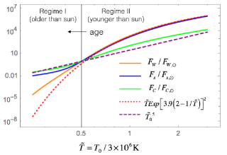
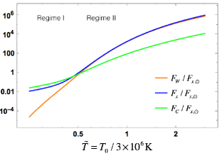
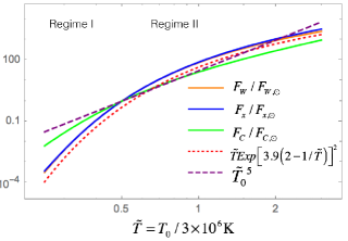
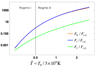
Figure 1: Panel $a$ shows $F_{W1}/F_{W1,\odot}$ (blue); $F_{C}/F_{C,\odot}$ (green); $l_{x}=F_{x}/F_{x,\odot}$ (orange); ${\tilde{T}}^{5}$ (purple dashed); ${\tilde{T}}Exp\left[-3.9\left({1\over{\tilde{T}}}-{3\times 10^{6}{\rm K}\over T_{0,\odot}}\right)\right]^{2}$ (red dotted). The y-axis is in units of the solar value for each quantity. Regimes I and II are defined by their x-ray temperature with respect to the solar average value, namely, ${\tilde{T}}<0.5$ and ${\tilde{T}}>0.5$ respectively for ${\tilde{T}}_{\odot}=0.5$. Panel $b$ shows ${\mathcal{L}}_{X}$, ${\mathcal{L}}_{W}$, and ${\mathcal{L}}_{C}$ all normalized to ${\mathcal{L}}_{X\odot}$ showing that coronal equilibrium for Regime II leads to ${\mathcal{L}}_{X}\simeq{\mathcal{L}}_{W}$.. Panels a and b show that ${\mathcal{L}}_{C}$ is subdominant for most all of regime II but dominant in most of regime I where the wind is correspondingly subdominant. Panels c and d have the same information as panels a and b but for a case in which the last exponent of Eqn. (16) is reduced by a factor of $2$, showing that the power-law fit $l_{x}\sim{\dot{m}}\sim{\tilde{T}}^{5}$ is not a bad approximation to $\dot{m}$ and $l_{x}$ for $0.5\leq{\tilde{T}}\leq 2$. In all panels we have used $\tilde{\Theta}=0.1$ (see text).

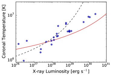
Figure 2: Comparison of coronal equilibrium temperature $T_{0}$ vs. x-ray luminosity from Eq.21 compared to data (Johnstone et al. 2015). The solid and dashed curves respectively correspond to the equilibrium temperatures for solar minimum and maximum, $T_{x,\odot 1}=0.97\times 10^{6}$K and $T_{x,\odot 2}=2.57\times 10^{6}$K (Johnstone et al. 2015). The plot shows that Eq. (21) is consistent with the data.

4.2 X-ray luminosity as function of magnetic field strength

Having established that $l_{x}\simeq{\dot{m}}$ in regime II, we now connect both of these quantities to the source of magnetic energy. Blackman & Thomas (2015) estimated $\mathcal{L}_{X}$ from the dynamo-produced magnetic energy rising up through the convection zone. To accommodate our present result that that 1/2 of source magnetic energy goes into $\mathcal{L}_{X}$, the relevant expression becomes

$$\begin{array}[]{r}\mathcal{L}_{X}\simeq 0.5\mathcal{L}_{mag}\simeq 0.5{B^{2}u_{b}\over 8\pi}\Theta r_{c}^{2}={1\over 3}\left({B^{2}\over 8\pi}\right)^{2}{\Theta r_{c}^{2}\over\rho v},\end{array}$$ (24)

where $B\sim{B}_{\phi}$ and $\Theta/4\pi$ is the solid angle fraction through which the field rises (proportional to, if not equal to $\tilde{\Theta}$ of the previous section), and we have used the expression for $u_{b}$ below Eq. (12). Using Eq. (13) in Eq. (24) then gives

$$\begin{array}[]{r}{\mathcal{L}_{x}\over\mathcal{L}_{*}}\simeq\left({L_{\alpha}\over r_{c}}\right)^{2/3}\left({s^{1/3}\over 1+s{\tilde{R}o}}\right)^{2}\Theta\left({3\pi\over 8}\right)^{1\over 3}\left({q_{\alpha}cos\theta_{s}\over 6}\right)^{2/3},\end{array}$$ (25)

where we have invoked $\mathcal{L}_{*}\simeq 4\pi r_{c}^{2}\rho{v^{3}},$ the luminosity associated with the convective heat flux through the convection zone (Shu, 1992). For the sun ${\tilde{R}o}\sim 2$ and $L_{\alpha}\sim 2r_{c}/5$.

We posit that $\Theta/4\pi\sim a_{spt}$ the areal fraction through which the strongest buoyant fields penetrate, approximately equal to the areal fraction of sunspots. For the sun $a_{spt,\odot}\mathrel{\hbox to0.0pt{\lower 4.0pt\hbox{\hskip 1.0pt$\sim$}\hss}\raise 1.0pt\hbox{$<$}}0.005$ (Solanki & Unruh, 2004). We allow $\Theta$ to depend on $\mathcal{L}_{X}/\mathcal{L}_{*}$ and take $\Theta=\Theta_{\odot}[({\mathcal{L}}_{X}/{\mathcal{L}}_{\odot})/({\mathcal{L}}_{X\odot}/{\mathcal{L}_{\odot}})]^{\lambda}$ (Blackman & Thomas, 2015). For $\lambda=1/3$, this implies that a factor of $10^{3}$ increase in the x-ray to bolometric luminosity ratio would imply $\Theta/4\pi=10a_{set,\odot}<0.1$, making self-consistent our assumption that ${\tilde{\Theta}}\leq 0.1$ above Eq. (19) if $\Theta\sim{\tilde{\Theta}}$. Combining with Eq. (25) we then have for ${\mathcal{L}}_{*}={\mathcal{L}}_{\odot}$

$$l_{x} \equiv {1\over 1.4-0.4t}\left({s\over s_{\odot}}\right)^{2\over 3(1-\lambda)}\left({{1+s_{\odot}{\tilde{R}o}}\over{1+s{\tilde{R}o}}}\right)^{2\over 1-\lambda}$$ (26)

$$= b_{r}^{4\over 1-\lambda},$$

where the factor $(1.4-0.4t)^{-1}$ approximates the increase in sun-like bolometric luminosity with time $t$ in unit of solar age (Gough, 1981), and the latter equality of Eq. (26) follows from Eq. (13) of Blackman & Thomas (2015) who showed that $0\leq\lambda\leq 1/3$ corresponds to $2\leq\zeta\leq 3$ (in Eq 1) in the unsaturated rotator regime. Increasing $\lambda$ increases the saturated $l_{x}$. Eq. (26) implies that $g_{L}(t)=(1.4-0.4t)^{\lambda-1\over 4}$ in Eq. (14).

5 Angular Momentum Evolution

In the previous sections, we have made theoretical progress by coupling the magnetic field strength, x-ray emission and mass-loss. To finally compute the global time-evolution of these quantities we need to know how our mass-loss rates and magnetic field strengths give rise to a torque on the star and spin it down. For simplicity we adopt a simple analytic formalism, although coupling with more detailed MHD simulations should be possible in the future.

Physically, we consider the Parker spherical wind solution to propagate along radial large scale fields out to the Alfvén radius where the toroidal field and radial field start to become comparable in the equatorial plane. We assume that the thermal energy driving the Parker wind is sourced via magnetic dissipation such that magnetic energy need not appear explicitly in the radial momentum equation for the wind. We correspondingly assume that the large scale Poynting flux does not contribute significantly to the wind acceleration. This is reasonable as long as the speed at the sonic point computed from the Parker wins is larger than the Michel velocity (Lamers & Cassinelli, 1999), which is self-consistently satisfied for the full range of our present solutions. We consider the angular momentum loss to be determined by that from the equatorial plane (Weber & Davis, 1967).

5.1 Angular momentum and toroidal field

Over a time scale shorter than the stellar spin-down time, the quasi-steady angular momentum equation of the wind in the equatorial plane reduces to (Weber & Davis, 1967; Lamers & Cassinelli, 1999)

$$\partial_{r}(rU_{\phi})={B_{r}r^{2}\over{\dot{M}}}\partial_{r}(r^{2}B_{\phi}),$$ (27)

where $U_{\phi}(r)$ is the azimuthal wind speed. Volume integrating the constraint that $\nabla\cdot{\bf B}=0$, implies

$$B_{r}=B_{r\odot}(r_{\odot}/r)^{2},$$ (28)

and in combination with Eq. (27) implies the radial constancy of

$$\mathcal{A}=r\left(U_{\phi}-{r^{2}B_{r}B_{\phi}\over{\dot{M}}}\right)=r^{2}_{*}\left(\Omega_{*}-{r_{*}B_{r*}B_{\phi*}\over{\dot{M}}}\right),$$ (29)

where the last equation follows because $\mathcal{A}$ can be computed at any wind radius, including the base.

The radial Alfvén speed is

$$u_{A}\equiv{B_{r}\over\sqrt{4\pi\rho}}$$ (30)

and the Alfvén Mach number

$$M_{A}\equiv U_{r}/u_{A},$$ (31)

where $U_{r}(r_{A})=u_{A}$ defines the Alfvén radius $r_{A}$. The steady-state (on time scales short compared to the spin-down time) induction equation for the electric field $\bf E$ is $\nabla{\times}{\bf E}=0$ and in spherical coordinates for the equatorial plane implies

$$B_{\phi}=(-\Omega_{*}B_{r}+U_{\phi}B_{r})/U_{r},$$ (32)

Using Eqs. (30), (31), (32), and $\dot{M}=4\pi r^{2}\rho U_{r}$ in the first equality of (29) and solving for $U_{\phi}$ gives (e.g. Lamers & Cassinelli (1999))

$$U_{\phi}={\Omega r}\left({\mathcal{A}M_{A}^{2}\over r^{2}\Omega_{*}}-1\over{M_{A}^{2}-1}\right).$$ (33)

so that a finite $U_{\phi}$ at $r=r_{A}$ implies

$$\mathcal{A}=r_{A}^{2}\Omega_{*}.$$ (34)

Plugging Eq. (34) back in to Eq. (29) gives

$${r_{A}\over r_{*}}=\left(1-{r_{*}B_{r*}B_{\phi*}\over\dot{M}\Omega_{*}}\right)^{1/2}.$$ (35)

Eq. (35) depends on $B_{\phi*}$, the only quantity on the right side for which we do not so far have a scaling in terms of $\Omega_{*}$ or present day solar values. We need a separate equation for ${r_{*}\over r_{A}}$ that is independent of $B_{\phi*}$ in order to also obtain independent equations for both $B_{\phi*}$ and $r_{A}/r_{*}$ as a function of the present solar values. To obtain the needed equation we note that Eqs. (28), (30) and (2) imply

$${r_{A}^{2}\over r^{2}_{*}}={B_{r*}\over B_{r,A}}={B_{r*}\over(4\pi\rho(r_{A}))^{1/2}u_{A}}={B_{r*}r_{A}\over{\dot{M}}^{1/2}u_{A}^{1/2}},$$ (36)

or

$${r_{A}\over r_{*}}={B_{r*}r_{*}\over{\dot{M}}^{1/2}u_{A}^{1/2}}={b_{r*}\over{\dot{m}}^{1/2}{\tilde{u}}_{A}^{1/2}}{B_{r\odot}r_{*}\over{\dot{M}}_{\odot}^{1/2}u_{A\odot}^{1/2}},$$ (37)

where ${\tilde{u}}_{A}\equiv{u_{A}\over u_{A\odot}}$ and we have used the definitions of $\dot{m}$ and $b_{r}$ from Eqs. (14) and (21). Rearranging Eq. (35) and using Eq. (37) then gives

$$b_{\phi*} \equiv {B_{\phi*}\over B_{\phi\odot}}$$ (38)

$$= -{{\dot{M}}\Omega_{*}\over r_{*}B_{r*}B_{\phi\odot}}\left[{r_{A}^{2}\over r_{*}^{2}}-1\right]$$

$$= -{{\dot{m}}\omega_{*}\over b_{r*}}{{\dot{M}}_{\odot}\Omega_{\odot}\over r_{*}B_{r\odot}B_{\phi\odot}}\left[{r_{A}^{2}\over r_{*}^{2}}-1\right],$$

where $\omega_{*}\equiv\Omega/\Omega_{\odot}$. The needed expression for $u(r_{A})=u_{A}$ for use in Eq. (37) (and thus in Eq. (38)) can be approximated from the two asymptotic forms Eqs. (6) and (7) taken at $r=r_{A}$. These latter two expressions then normalized to $u_{A,\odot}$ (the value for the present day sun) can then be combined in the form

$${\tilde{u}}_{A}(t)\equiv u_{A}/u_{A\odot}=\sqrt{T\over T_{\odot}}\times$$ (39)

$$\!\!\!\!\!\!\!\!\!\!\!\max\left\{\exp\left[2\left({r_{s\odot}\over r_{A\odot}}\right)\left(1-{T_{\odot}\over T}{r_{A\odot}\over r_{A}}\right)\right];\sqrt{{Ln\left[{T\over T_{\odot}}{r_{A}\over r_{*}}{r_{*}\over r_{s\odot}}\right]\over Ln\left[{r_{A\odot}\over r_{s\odot}}\right]}}\right\}.$$

In practice, the sonic radius is always below the Aflvén radius for our purposes so the latter of the two approximations actually suffices for present purposes.

5.2 Time-evolution of angular velocity

Over time scales $>>r_{s}/U_{r}$, the star will spin-down by angular momentum loss into the wind via the magnetic field. From conservation of angular momentum, the evolution of the stellar angular velocity is then

$${\dot{\Omega}}=-{q\over 0.059Mr_{*}^{2}}{\mathcal{A}{\dot{M}}}=-{{q\dot{M}}\Omega_{*}\over 0.059M}{r_{A}^{2}\over r_{*}^{2}}=-{q\Omega_{*}\over 0.059M}{B_{r}^{2}r^{2}_{*}\over u_{A}},$$ (40)

where ${{\mathcal{I}}_{\odot}\over M_{\odot}r_{\odot}^{2}}=0.059$, ${\mathcal{I}}_{\odot}$ is the moment of inertia of the sun, and the inertial parameter $q>1$ is a numerical factor to reduce this by an amount that depends on internal angular momentum transport and the fraction of the star to which the field is anchored. We have used Eq. (34) and Eq. (37) for the second and third equalities in Eq. (40) respectively. (We note that the form of Eq (40) can also be recovered from Eq. 9 of Matt et al. (2012), by setting our $q=K_{1}^{2}$ therein and taking $f^{2}<<K_{2}^{2}$ and $m=1/2$ in that equation). Scaling to present solar values, Eq. (40) in dimensionless form becomes

$${d\omega_{*}\over d\tau}\equiv-{\omega_{*}}{qb_{r}^{2}\over m{\tilde{u}}_{A}}{B_{r\odot}^{2}\Omega_{\odot}\tau_{\odot}\over M_{\odot}u_{A\odot}},$$ (41)

where $\tau_{\odot}$ is the present day solar age.

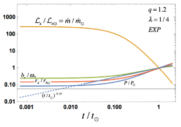
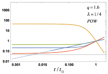
Figure 3: The panels (a,b,c,d) each show plots of $\mathcal{L}_{X}/\mathcal{L}_{\odot}\sim\dot{m}$ (orange), $b_{r}/\omega_{*}$ (green), $r_{A}/r_{A\odot}$ (red), and $P/P_{\odot}$(blue curved) compared with the Skumanich law (blue straight) for different $q$ and $\lambda$. The latter curve has been extended as a dotted line in the region where it is no longer applicable to observations. All panels have same colour code. Panels abc corresponds to solutions were Eqn (21) is used to relate $l_{x}$ and $T$ whereas panel d applies when the last exponent in Eqn (16) is reduced by a factor of $2$ and the power-law approximation $l_{x}\sim{\dot{m}}\sim{\tilde{T}}^{5}$ is used.

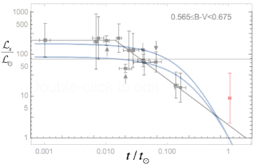
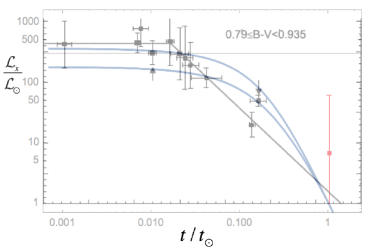
Figure 4: The two panels show plots of ${\mathcal{L}}_{x}/{\mathcal{L}}_{bol}$ vs. time (blue lines) overplayed with plots from Jackson et al. (2012) who fit the black lines to the black data points from open clusters selected by color index range (shown on the plot). The red point is a reference field star not used in their fits. The top and bottom curves of the top panel correspond to $l_{x}$ for $q=1.0$ and $1.1$ and in the bottom panel to $q=1.1$ and $q=1.2$ respectively. Because our solutions are for fixed mass equal to $M_{\odot}$ but the color of stars of given mass can change with age, there is degeneracy a single star would not evolve in a plot for a singe color index range. The solar colour index decreases with age and so we simply took plots from the color index ranges appropriate for the present sun ($B-V=0.69$ early sun ($B-V=0.83$) to show examples of how our solutions mesh with data. All curves use $\lambda=1/3$.

6 Time-Dependent Solutions

Focusing on the time evolution of a star that emerges with the current solar properties at the sun’s age, we assume that the radius, mass, and thermal convection time of the star do not evolve from the early main sequence to the present time. Eqs. (41), (26), (21), and (38), along with (37) and (39) and the present day solar properties then form a complete set of equations that can be solved for the coupled time evolution of $\omega_{*},b_{r},l_{x}\sim{\dot{m}}$, $b_{\phi}$, and $u_{A}$.

6.1 Basic Properties of the Holistic Solutions

The free parameters of the model are essentially $s$, $q$ and $\lambda$ (with the measured solar properties as boundary conditions). We fix the shear parameter $s$ at $s=8.3$ as in Blackman & Thomas (2015) because this value makes the transition from saturated to unsaturated regime at $s{\tilde{R}o}=1$ or $1/s=0.12$ consistent with best fit to observations (Wright et al., 2011). However the transition is smooth and the asymptotic regimes ${\tilde{R}o}>>1$, and ${\tilde{R}o}<<1$ are not so sensitive to it. It depends on the physics of internal differential rotation. We focus instead on $q$ and $\lambda$.

Fig. 3a-c show the time evolution (in units of solar age) of $l_{x}\sim{\dot{m}},1/\omega_{*},r_{A}/r_{A\odot},$ and $b_{r}/\Omega$ normalized to the present solar values for values of the inertial parameter $q$ and $\lambda$ as shown. In our simple model we treat $q$ as a free parameter, but note that physical values require $q>1$ and the solutions are quite sensitive to the specific choice. As $q$ is increased, the lower effective momentum of inertia leads to a faster spin-down and thus the early time $l_{x}$ is higher than for lower $q$ to evolve to the same solar values at the sun’s age. The physically reasonable range of $1\leq q\leq 2$ works best as we discuss below with respect to Fig 3. In reality, $q$ is likely a function of time and would evolve if the internal rotational coupling of core and envelope evolves. We have assumed that $q$ is a constant for simplicity. Fig 3d shows the same information as the previous panels but for a case associated with Figs. 1c & d in which the exponent in Eqn (16) is reduced by a factor of 2.

The plots of Fig. 3 also show the modified Skumanich law (Mamajek, 2014) $1/\Omega=t^{0.55}$ which is known to fit the data well in the unsaturated regime, and can be compared with our dynamical solution. The Skumanich law does not apply to stars much younger than $5\times 10^{7}$yr (Gallet & Bouvier, 2013) but we show its extension there as well, highlighting the fact that our solutions give longer periods at earlier times, perhaps consistent with the ”slow rotator” cases of Gallet & Bouvier (2013). The physics of our model is insufficient for stars with dynamically influential disks, which means inapplicable for ages below $~{}5\times 10^{6}$yr. In general, as $q$ is increased above unity for fixed $\lambda$ the concavity of our solutions compared to the Skumanich law increases at late times and the intersection between the two curves shifts to small times.

Finally, we note that the purple curves of Fig 3. show that $b_{r}/\omega_{*}$ remains within an order of unity solar-like star for our solutions over for at least 3 orders of magnitude in $\tau$ and remains more constant than the blue curves over both the full time range. This results because for the unsaturated regime ( ${\tilde{R}o}>>0.13)$, $B\propto\Omega^{1/2}$ from Eqn. (13) This is in general agreement with the Vidotto et al. (2014) result mentioned in Sec. 1, that the field and angular velocity scale similarly with age.

6.2 Example Comparisons of $l_{x}$ vs. Age with data

Fig 4. shows the $l_{x}$ solutions plotted in same form as Fig. 3 for two values of $q$ in each panel overlayed with data plots of (Jackson, Davis & Wheatley, 2012) for luminosity and age binned by $B-V$ colour index. The figure illustrates of how the solutions can connect to the data and what is possible for further work. Even though colour might be intended to select a mass range (Pizzolato et al., 2003), the evolution of colour with age implies that a single star of fixed mass would not be pinpointed in age using a fixed colour index. In the figure, we compare our fixed mass ($=M_{\odot}$) solutions for for the parameters indicated with two photometric classes. The two classes chosen correspond to the color range associated with the present sun ($B-V=0.69$) and the color range corresponding to the early sun ($B-V=0.83$) In the two panels we show solutions for $q=1.1$ (top) and $q=1.2$ bottom, for the two $B-V$ photometric bins. More detailed modeling which includes solutions for a range of masses and color variations for a given is desired to match theory with data from stellar populations.

Fig 4 shows that the general trends of ${\mathcal{L}}_{X}/{\mathcal{L}}_{bol}$ are broadly captured by our model for reasonable ranges of $q$. However, if $q$ is fixed such that the solution fits the saturated early time regime of $l_{x}$, then the curves tend to overshoot in the unsaturated late-time regime. Similarly lowering $q$ to capture the late time regime of the population then undershoots $l_{x}$ in the saturated regime. A better model could include $dq/dt<0$ so that more of the star is coupled to its angular momentum loss as the star ages. In addition, more detailed spin-down torque modeling that produces a different power of $B_{r}$ in Eq. (40) (e.g. Matt et al. (2015)) can modify the turnover locus and curve shape. The next subsection shows that small variations in the average equilibrium temperature for solar-like stars can also affect the shape of $l_{x}$.

There is some degeneracy between increasing $\lambda$ instead of increasing $q$. The former implies a stronger dependence of $l_{x}$ on $\Theta$ (as discussed at the end of Sec 2.), and thus a stronger dependence of $l_{x}$ on rotation and time in the unsaturated rotation regime. Eq. (26) shows that $l_{x}\propto{\tilde{R}o}^{2\over 1-\lambda}$ and observations (Wright et al., 2011) then require $0\leq\lambda\leq 1/3$. Blackman & Thomas (2015) showed that $\lambda=1/3$ seems to match the shape of the overall averaged $l_{x}({\tilde{R}o})$ curve averaged over stars of different masses and ages compared to $\lambda=0$. The higher value of $\lambda$ raises $l_{x}$ in the saturated regime, and steepens it in the unsaturated regime. However for a single star such as the sun, the saturated $l_{x}$ could be lower than the average over a potpourri of late-type stars. More observational constraints on $\Theta$ are needed. The generic effect of changing $\lambda$ is captured in Fig. (3)ab.

6.3 Effect of varying $T_{x\odot}$: prediction of increased spread in $l_{x}$ with stellar youth:

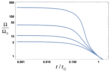
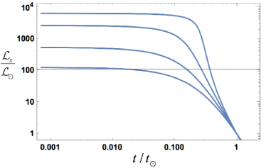
Figure 5: Our solutions for $\omega_{*}$ (panel a) and $l_{x}$ (panel b) predict a broader spread in these quantities at early times compared to late times if we make small changes in the coronal equilibrium temperature normalization for the sun at the current age. For all curves, $\lambda=1/3$, $q=1.2$, but from bottom to top in each panel we have used respectively ${\tilde{T}}_{0,\odot}={1\over 1.6},{1\over 2.0},{1\over 2.2},{1\over 2.4}$. The choice ${\tilde{T}}_{0,\odot}=1/2$ corresponds to $T_{x,\odot}=1.5\times 10^{6}$K and is that which was used previously in Section 4.

One other important implication of our calculations is the prediction that the spread in $\omega$ and $l_{x}$ should increase with decreasing age for a given stellar mass if we allow small changes to the coronal equilibrium temperature at the solar age. This is shown in Fig 5 and agrees with the trends reported in Gallet & Bouvier (2013) The bottom and top curves in each panel of Fig 5 correspond to the extremes ${\tilde{T}}_{0\odot}={1\over 1.6}$ and ${\tilde{T}}_{0\odot}={1\over 2.4}$ respectively. These extremes differ by less than a factor of 2, and are smaller than the reported variation in the Sun’s corona temperature (e.g. Johnstone et al., 2015).

The sensitive dependence of $\omega_{*}$ and $l_{x}$ to ${\tilde{T}}_{0\odot}$ at early times can be traced to the fact that in Eq. (21), the exponent is such that $l_{x}$ depletes more rapidly toward $l_{x}\sim 1$ for smaller $T_{0\odot}$. Then when coupled to the time dependence, $l_{x}$ increases with $\omega_{*}$ in the unsaturated regime, both of these two quantites have larger maxima in the saturated regime at early times to arrive at the solar values at the sun’s age.

Note also that in Eq. 41, the ratio of $b_{r}^{2}(t)/u_{A}(t)$ is less sensitive to $\omega_{*}(t)$ in the unsaturated regime than is $\omega_{*}(t)^{-1/2}$. Thus $\omega_{*}(t)$ evolves more sharply with the ideal Skumanich law but may still produce an ”apparent” correspondence (see Fig 3) if error bars on rotation periods are with a factor of 2 (highlighting the need for more data). From Eqs. (14) and (26), we see that $l_{x}\propto\omega_{*}^{2\over 1-\lambda}\sim\omega_{*}^{3}$ for $\lambda=1/3$ in the unsaturated regime so that the time evolution of $l_{x}$ is more sensitive to $\omega_{*}$ than $\omega_{*}$ itself, explaining why the spread from the top curve to the bottom curve is larger for luminosity than for $\omega_{*}$

7 Conclusion

To solve for the coupled main sequence stellar evolution of x-ray luminosity, rotation, mass loss rate, and mean magnetic field strength, we have constructed a simple model combining an isothermal Parker wind with sourcing of the needed thermal energy by dynamo generated magnetic fields. The dynamo produced fields are estimated from a modern saturation paradigm based on magnetic helicity evolution and a physically motivated replacement of the convection time in the dynamo coefficients by the shear time for fast rotators. The latter had been previously used in an effort to explain the $l_{x}(Ro)$ behaviour of late-type stars but without the time evolution. The division of the magnetic sourcing into radiation vs. wind is determined by the consequences of assuming energy balance between heating, cooling and mass loss in the corona on time scales short compared to the the spin down. We find that ${\mathcal{L}}_{X}\sim{\mathcal{L}}_{W}$ for the appropriate range of coronal temperatures, masses and radii of early-type stars.

The time dependent solutions we obtain exhibit broad-brush agreement with observational trends. This includes time evolution of x-ray luminosities, magnetic field, and rotation period, and the approximate scaling of mass loss rate with x-ray luminosity. We have limited ourselves to a minimalist holistic time-dependent model as a framework for more detailed models which seems justified, given the previous lack of unification of the aforementioned pieces in single theory and the need for more observational data.

We have primarily focused the time evolution of stellar properties of stars younger than the present sun up to the present day solar values assuming that over the course of the main sequence evolution, the mass and radius are fixed. The same approach for stars of other initial masses and radii normalized to any currently measured fidiucial values would be of interest for future work. Then a population of curves for a range of stars could be generated and averaged properties across stars could be determined. We have shown that a population of solar-type stars whose solar-age coronal equilibrium temperature deviates by less than a factor of two, would produce a broad spread of x-ray luminosities and rotation periods in youth, converging to a narrow range in old age, seemingly consistent with observations (Gallet & Bouvier, 2013).

For stars older than the sun, our model suggests that conductive losses are relatively more important than wind losses than for younger stars (compare regimes I and II of Fig. 1b). This would in turn imply a reduction in angular momentum loss, possibly helping to explain the flattening in the observed period-age relation for old stars (van Saders et al., 2016). Exploring ”regime I” further, and the implications for angular momentum loss are topics for future work.

More detailed extensions of our framework could include deviations from spherical symmetry for the wind solution, more explicit modeling of closed and open fraction of field lines, more detailed models of mass loss (e.g. Suzuki et al., 2013) and spin-down torques (e.g. Matt et al., 2015); inclusion of magnetic contributions to the wind radial momentum equation for fast rotators, a more detailed time dependent dynamo solution, and time dependent modeling of convection and internal stellar structure. The latter may help predict/constrain the free parameter $\lambda$, which may also be extractable empirically now from Kepler data (McQuillan, Mazeh & Aigrain, 2014). Understanding the mechanisms and dynamics of angular momentum coupling and decoupling between core and envelope may also particularly important (Gallet & Bouvier, 2013; Amard et al., 2016). Further extensions to include disk-star interactions might be further desirable to extend the framework to pre-main sequence evolution that would predict the ”initial” conditions for the post-disk main sequence evolution.

With each additional complexity also comes additional caution that the ingredients that add to the complexity may themselves not be well understood. For example, how dynamos work in stars, where in the star the field is actually amplified and anchored, and how the interior dynamo and anisotropic convection evolve with time and connect to the coronal field remain matters of active research, even for steady state conditions. In this sense, there is value both in minimalist approaches as well as detailed modeling.

References

- Amard et al. (2016) Amard L., Palacios A., Charbonnel C., Gallet F., Bouvier J., 2016, A&A, 587, A105
- Aschwanden (2004) Aschwanden M. J., 2004, Physics of the Solar Corona. An Introduction. Praxis Publishing Ltd; Chichester, UK
- Athay (1990) Athay R. G., 1990, ApJ, 362, 364
- Baliunas et al. (1998) Baliunas S. L., Donahue R. A., Soon W., Henry G. W., 1998, in Astronomical Society of the Pacific Conference Series, Vol. 154, Cool Stars, Stellar Systems, and the Sun, Donahue R. A., Bookbinder J. A., eds., p. 153
- Barker, Dempsey & Lithwick (2014) Barker A. J., Dempsey A. M., Lithwick Y., 2014, ApJ, 791, 13
- Blackman (2015) Blackman E. G., 2015, Sp Sci. Rev., 188, 59
- Blackman & Field (2002) Blackman E. G., Field G. B., 2002, Physical Review Letters, 89, 265007
- Blackman & Thomas (2015) Blackman E. G., Thomas J. H., 2015, MNRAS, 446, L51
- Brandenburg & Subramanian (2005) Brandenburg A., Subramanian K., 2005, Phys. Reports, 417, 1
- Christensen, Holzwarth & Reiners (2009) Christensen U. R., Holzwarth V., Reiners A., 2009, Nature, 457, 167
- Cox (2000) Cox A. N., 2000, Allen’s astrophysical quantities. New York: AIP and Springer
- Cranmer (2012) Cranmer S. R., 2012, Sp Sci. Rev., 172, 145
- Cranmer & Saar (2011) Cranmer S. R., Saar S. H., 2011, ApJ, 741, 54
- Durney & Robinson (1982) Durney B. R., Robinson R. D., 1982, ApJ, 253, 290
- Epstein & Pinsonneault (2014) Epstein C. R., Pinsonneault M. H., 2014, ApJ, 780, 159
- Gallet & Bouvier (2013) Gallet F., Bouvier J., 2013, A&A, 556, A36
- Gilliland et al. (2010) Gilliland R. L. et al., 2010, PASP, 122, 131
- Gough (1981) Gough D. O., 1981, Solar Physics, 74, 21
- Hearn (1975) Hearn A. G., 1975, Astron. & Astrophys., 40, 355
- Holzwarth & Jardine (2007) Holzwarth V., Jardine M., 2007, A&A, 463, 11
- Jackson, Davis & Wheatley (2012) Jackson A. P., Davis T. A., Wheatley P. J., 2012, MNRAS, 422, 2024
- Johnstone et al. (2015) Johnstone C. P., Güdel M., Brott I., Lüftinger T., 2015, A&A, 577, A28
- Kippenhahn, Weigert & Weiss (2012) Kippenhahn R., Weigert A., Weiss A., 2012, Stellar Structure and Evolution. Springer
- Krause & Raedler (1980) Krause F., Raedler K. H., 1980, Mean-field magnetohydrodynamics and dynamo theory. Pergamon Press; New York
- Lamers & Cassinelli (1999) Lamers H. J. G. L. M., Cassinelli J. P., 1999, Introduction to Stellar Winds. Cambridge Univ. Press
- Mamajek (2014) Mamajek E. E., 2014, Figshare, http://dx.doi.org/10.6084/m9.figshare.1051826
- Mamajek & Hillenbrand (2008) Mamajek E. E., Hillenbrand L. A., 2008, ApJ, 687, 1264
- Matt & Pudritz (2008) Matt S., Pudritz R. E., 2008, ApJ, 678, 1109
- Matt et al. (2015) Matt S. P., Brun A. S., Baraffe I., Bouvier J., Chabrier G., 2015, ApJL, 799, L23
- Matt et al. (2012) Matt S. P., MacGregor K. B., Pinsonneault M. H., Greene T. P., 2012, ApJL, 754, L26
- McQuillan, Mazeh & Aigrain (2014) McQuillan A., Mazeh T., Aigrain S., 2014, ApJS, 211, 24
- Micela et al. (1985) Micela G., Sciortino S., Serio S., Vaiana G. S., Bookbinder J., Golub L., Harnden, Jr. F. R., Rosner R., 1985, ApJ, 292, 172
- Mitra et al. (2014) Mitra D., Brandenburg A., Kleeorin N., Rogachevskii I., 2014, MNRAS, 445, 761
- Moffatt (1978) Moffatt H. K., 1978, Magnetic field generation in electrically conducting fluids. Cambridge Univ. Press
- Montesinos et al. (2001) Montesinos B., Thomas J. H., Ventura P., Mazzitelli I., 2001, MNRAS, 326, 877
- Morgenthaler et al. (2011) Morgenthaler A., Petit P., Morin J., Aurière M., Dintrans B., Konstantinova-Antova R., Marsden S., 2011, Astronomische Nachrichten, 332, 866
- Noyes et al. (1984) Noyes R. W., Hartmann L. W., Baliunas S. L., Duncan D. K., Vaughan A. H., 1984, ApJ, 279, 763
- Owen & Adams (2014) Owen J. E., Adams F. C., 2014, MNRAS, 444, 3761
- Owen & Wu (2013) Owen J. E., Wu Y., 2013, ApJ, 775, 105
- Pallavicini et al. (1981) Pallavicini R., Golub L., Rosner R., Vaiana G. S., Ayres T., Linsky J. L., 1981, ApJ, 248, 279
- Parker (1958) Parker E. N., 1958, ApJ, 128, 664
- Parker (1979) Parker E. N., 1979, Cosmical magnetic fields: Their origin and their activity. Oxford Univ. Press
- Pipin (2015) Pipin V. V., 2015, MNRAS, 451, 1528
- Pizzolato et al. (2003) Pizzolato N., Maggio A., Micela G., Sciortino S., Ventura P., 2003, A&A, 397, 147
- Pneuman & Kopp (1971) Pneuman G. W., Kopp R. A., 1971, Solar Physics, 18, 258
- Pouquet, Frisch & Leorat (1976) Pouquet A., Frisch U., Leorat J., 1976, Journal of Fluid Mechanics, 77, 321
- Randich (2000) Randich S., 2000, in Astronomical Society of the Pacific Conference Series, Vol. 198, Stellar Clusters and Associations: Convection, Rotation, and Dynamos, Pallavicini R., Micela G., Sciortino S., eds., p. 401
- Reiners & Mohanty (2012) Reiners A., Mohanty S., 2012, ApJ, 746, 43
- Reiners, Schüssler & Passegger (2014) Reiners A., Schüssler M., Passegger V. M., 2014, ApJ, 794, 144
- Schrijver & Zwaan (2000) Schrijver C. J., Zwaan C., 2000, Solar and Stellar Magnetic Activity. Cambridge Univ. Press
- Shu (1992) Shu F. H., 1992, The physics of astrophysics. Volume II: Gas dynamics. University Science Books
- Shukurov et al. (2006) Shukurov A., Sokoloff D., Subramanian K., Brandenburg A., 2006, A&A, 448, L33
- Skumanich (1972) Skumanich A., 1972, ApJ, 171, 565
- Solanki & Unruh (2004) Solanki S. K., Unruh Y. C., 2004, MNRAS, 348, 307
- Subramanian & Brandenburg (2006) Subramanian K., Brandenburg A., 2006, ApJL, 648, L71
- Suzuki et al. (2013) Suzuki T. K., Imada S., Kataoka R., Kato Y., Matsumoto T., Miyahara H., Tsuneta S., 2013, PASJ, 65, 98
- Tarduno, Blackman & Mamajek (2014) Tarduno J. A., Blackman E. G., Mamajek E. E., 2014, Physics of the Earth and Planetary Interiors, 233, 68
- Tobias et al. (2001) Tobias S. M., Brummell N. H., Clune T. L., Toomre J., 2001, ApJ, 549, 1183
- van Saders et al. (2016) van Saders J. L., Ceillier T., Metcalfe T. S., Silva Aguirre V., Pinsonneault M. H., García R. A., Mathur S., Davies G. R., 2016, Nature, 529, 181
- van Saders & Pinsonneault (2013) van Saders J. L., Pinsonneault M. H., 2013, ApJ, 776, 67
- Vidotto et al. (2016) Vidotto A. A. et al., 2016, MNRAS, 455, L52
- Vidotto et al. (2012) Vidotto A. A., Fares R., Jardine M., Donati J.-F., Opher M., Moutou C., Catala C., Gombosi T. I., 2012, MNRAS, 423, 3285
- Vidotto et al. (2014) Vidotto A. A. et al., 2014, MNRAS, 441, 2361
- Vilhu (1984) Vilhu O., 1984, A&A, 133, 117
- Weber & Davis (1967) Weber E. J., Davis, Jr. L., 1967, ApJ, 148, 217
- Weber, Fan & Miesch (2013) Weber M. A., Fan Y., Miesch M. S., 2013, Solar Physics, 287, 239
- Wood et al. (2014) Wood B. E., Müller H.-R., Redfield S., Edelman E., 2014, ApJL, 781, L33
- Wood et al. (2005) Wood B. E., Müller H.-R., Zank G. P., Linsky J. L., Redfield S., 2005, ApJL, 628, L143
- Wright et al. (2011) Wright N. J., Drake J. J., Mamajek E. E., Henry G. W., 2011, ApJ, 743, 48