Quantum modularity and complex Chern-Simons theory

Abstract.

The Quantum Modularity Conjecture of Zagier predicts the existence of a formal power series with arithmetically interesting coefficients that appears in the asymptotics of the Kashaev invariant at each root of unity. Our goal is to construct a power series from a Neumann-Zagier datum (i.e., an ideal triangulation of the knot complement and a geometric solution to the gluing equations) and a complex root of unity $\zeta$. We prove that the coefficients of our series lie in the trace field of the knot, adjoined a complex root of unity. We conjecture that our series are those that appear in the Quantum Modularity Conjecture and confirm that they match the numerical asymptotics of the Kashaev invariant (at various roots of unity) computed by Zagier and the first author. Our construction is motivated by the analysis of singular limits in Chern-Simons theory with gauge group $SL(2,\mathbb{C})$ at fixed level $k$, where $\zeta^{k}=1$.

1. Introduction

1.1. Quantum modular forms

Quantum modular forms are fascinating objects introduced by Zagier [Zag10]. In the simplest formulation, a quantum modular form is a complex valued function $f$ on the set of complex roots of unity that comes equipped with a suitable formal power series expansion $\phi_{\zeta}(\hbar)\in\mathbb{C}[\![\hbar]\!]$ at each complex root of unity $\zeta$. Usually $f$ is given explicitly. On the other hand, the power series $\phi_{\zeta}$, although uniquely determined by $f$, are not easy to obtain.

One of the most interesting examples of quantum modular forms is conjectured to be the logarithm of the Kashaev invariant of a knot. This is Zagier’s Quantum Modularity Conjecture [Zag10]. Evidence for this conjecture includes ample numerical computations performed by Zagier and the first author [GZ] as well as a proof in the case of the $4_{1}$ knot [GZ].

Our goal is to construct an explicit formula for the power series that appear in the Quantum Modularity Conjecture of a knot. We highlight some features of our results.

(a) The formulas for our series $\phi_{\gamma,\zeta}(\hbar)$ use as input a complex root of unity $\zeta$ and Neumann-Zagier datum $\gamma$, i.e., an ideal triangulation of a knot complement and a geometric solution to the gluing equations. Such a datum is readily available from SnapPy.

(b) Our series have arithmetically interesting coefficients; see Theorems 2.2 and 2.6.

(c) Our series lead to exact computations that match the numerically computed asymptotics of the Kashaev invariant at various roots of unity. The details of our computations are given in Section 5.

(d) Our construction is motivated by the analysis of singular limits in complex Chern-Simons theory, with gauge group $SL(2,\mathbb{C})$. Complex Chern-Simons theory depends on two coupling constants or levels $(k,\sigma)\in(\mathbb{Z},\mathbb{C})$ [Wit91], and the series $\phi_{\gamma,\zeta}(\hbar)$ at $\zeta=e^{2\pi i/k}$ is obtained by sending $\sigma\to k$ (while keeping $k$ fixed). We describe this limit in greater detail in Section 4, after introducing the definition of $\phi_{\gamma,\zeta}(\hbar)$ and proving its number-theoretic properties in Sections 2-3.

1.2. Zagier’s Quantum Modularity Conjecture

The Kashaev invariant of a knot $K$ is a sequence of complex numbers $\langle K\rangle_{N}$ indexed by a positive integer $N$ [Kas95]. Murakami-Murakami [MM01] identified the Kashaev invariant with an evaluation of the colored Jones polynomial $J_{K,N}(q)\in\mathbb{Z}[q^{\pm 1}]$ colored by the $N$-dimensional irreducible representation of $\mathfrak{sl}_{2}$:

$$\langle K\rangle_{N}=J_{K,N}(e^{\frac{2\pi i}{N}})\,.$$

Identifying the set of complex roots of unity with $\mathbb{Q}/\mathbb{Z}$, the Kashaev invariant can be extended to a translation-invariant function on $\mathbb{Q}$ by

(1) $$J^{0}_{K}:\mathbb{Q}\longrightarrow\mathbb{C},\qquad\alpha\mapsto J^{0}_{K}(\alpha)=J_{K,\mathrm{den}(\alpha)}(e^{2\pi i\alpha})$$

where $\mathrm{den}(a/c)=c$ when $c>0$ and $a,c$ are coprime. Obviously, we have $J^{0}_{K}(\alpha)=J^{0}_{K}(\alpha+1)$ for $\alpha\in\mathbb{Q}$.

The Quantum Modularity Conjecture [Zag10] predicts for each complex root of unity $\zeta$ the existence of a formal power series $\phi_{K,\zeta}(\hbar)\in\mathbb{C}[\![\hbar]\!]$ with the following property. Choose any $\begin{pmatrix}a&b\\ c&d\end{pmatrix}\in\mathrm{SL}(2,\mathbb{Z})$ with $c>0$ such that $\zeta=\exp(\frac{2\pi ia}{c})$. Let $X\to\infty$ in a fixed coset of $\mathbb{Q}/\mathbb{Z}$, and set $\hbar=2\pi i/(cX+d)$. Then there is an asymptotic expansion

(2) $$J^{0}_{K}\left(\frac{aX+b}{cX+d}\right)\sim J^{0}_{K}(X)\big{(}\tfrac{2\pi i}{\hbar}\big{)}^{3/2}e^{V/(c\hbar)}\phi_{K,\zeta}(\hbar)$$

where $V$ is the complex volume of $K$. Furthermore, the coefficients of $\phi_{K,\zeta}(\hbar)$ are conjectured to be algebraic integers of the following form:

• The coefficients of $\phi^{+}_{K,\zeta}(\hbar)=\phi_{K,\zeta}(\hbar)/\phi_{K,\zeta}(0)$ should be elements of the field $F_{K}(\zeta)$, where $F_{K}$ is the trace field of $K$.

• The constant term (under some mild assumptions on $F_{K}(\zeta)$) should factor as follows:

  (3) $$\phi_{K,k}(0)=\phi_{K,1}(0)\sqrt[k]{\varepsilon_{K}}\beta_{K,k}$$

  where $\phi_{K,1}(0)^{2}\in F_{K}(\zeta)$, $\varepsilon_{K}$ is a unit (i.e., an algebraic integer of norm $\pm 1$) in $F_{K}(\zeta)$ that depends only on the element of the Bloch group of $K$ (and $\zeta$), and $\beta_{K,k}\in F_{K}(\zeta)$.

The above unit is studied in [CGZ]. For a detailed discussion of the Quantum Modularity Conjecture, we refer the reader to [Zag10] and also [GZ] where a proof for the case of the $4_{1}$ knot (the simplest hyperbolic knot) is given.

The Quantum Modularity Conjecture includes the Volume Conjecture of Kashaev  [Kas95] and its refinement to all orders of $1/N$ conjectured by Gukov [Guk05] and by the second author [Gar08]. Indeed, when $\left(\begin{smallmatrix}a&b\\ c&d\end{smallmatrix}\right)=\left(\begin{smallmatrix}0&-1\\ 1&0\end{smallmatrix}\right)$ and $X=N\in\mathbb{N}$, we obtain that

(4) $$\overline{\langle K\rangle_{N}}=J^{0}_{K}\left(-\frac{1}{N}\right)\sim N^{3/2}e^{NV/(2\pi i)}\phi_{K,1}\left(\frac{2\pi i}{N}\right)\,.$$

The second author and Zagier numerically computed the Kashaev invariant and its asymptotics, exposing several coefficients of the series $\phi_{K,\zeta}(\hbar)$ for many knots, and giving numerical confirmation of the Modularity Conjecture. The results are summarized in [GZ].

A definition of the power series $\phi_{K,\zeta}(\hbar)$ in the Quantum Modularity Conjecture was missing, though. Motivated by this problem, in an earlier publication  [DG13a] (inspired by [DGLZ09]) the authors assigned to a Neumann-Zagier datum $\gamma$ (i.e., to an ideal triangulation of the knot complement, a geometric solution to the gluing equations and a flattening) a power series $\phi_{\gamma,1}(\hbar)$ and conjectured that it coincides with the series $\phi_{K,1}(\hbar)$. One advantage of the series $\phi_{\gamma,1}(\hbar)$ is the exact computation of its coefficients using standard SnapPy methods [CDW], together with finite sums of Feynman diagrams. In all cases we matched those coefficients with the numerically computed values of [GZ]. In [DG13a], it was shown that the constant term of $\phi_{\gamma,1}(\hbar)$ is a topological invariant, but to date the full topological invariance of $\phi_{\gamma,1}(\hbar)$ is unknown.

Finally, we ought to point out a close connection between our series $\phi_{\gamma,\zeta}(\hbar)$ and

• The radial asymptotics of Nahm sums at complex roots of unity. This connection was observed at $\zeta=1$ during conversations of the second author and Zagier in Bonn in the spring of 2012.

• The evaluations of one-dimensional state-integrals at rational points [GK13, GK14].

• The formula for an algebraic unit attached to an element of the Bloch group of a number field and a complex root of unity, appearing in (3) [CGZ].

These connections are not a coincidence; rather, they close a circle of ideas motivated by several years of work on asymptotics of hypergeometric sums, quantum invariants, and their geometry and physics.

2. The definition of $\phi_{\gamma,\zeta}$

2.1. Ideal triangulations and Neumann-Zagier data

Ideal triangulations were introduced by Thurston as an efficient way to describe (algebraically, or numerically) 3-dimensional hyperbolic manifolds. For a leisure introduction, the reader may consult Thurston’s original notes [Thu77], the exposition of Neumann–Zagier [NZ85] and Weeks [Wee05] and the documentation of SnapPy [CDW]. The shape of a 3-dimensional hyperbolic tetrahedra is a complex number $z\in\mathbb{C}\setminus\{0,1\}$. Letting $z^{\prime}=(1-z)^{-1}$ and $z^{\prime\prime}=1-z^{-1}$, the edges of an oriented ideal tetrahedron of shape $z$ can be assigned complex numbers according to Figure 1.

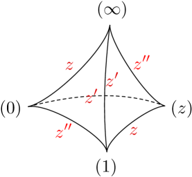
Figure 1. An ideal tetrahedron with a shape assignement.

Let $M$ be an oriented hyperbolic manifold with one cusp (for instance a hyperbolic knot complement) and $\mathcal{T}$ an ideal triangulation of $M$ containing $N$ tetrahedra. In [DG13a] the authors introduced a Neumann-Zagier datum of $\mathcal{T}$. The latter is a tuple $\gamma=(\mathbf{A},\mathbf{B},\nu,z,f,f^{\prime\prime})$ that consists of:

• Two matrices $\mathbf{A},\mathbf{B}\in\mathrm{GL}(N,\mathbb{Z})$ and a vector $\nu\in\mathbb{Z}^{N}$ encoding the coefficients of Thurston’s gluing equations for the triangulation ($N-1$ independent equations imposing trivial holonomy around edges, and one equation imposing parabolic holonomy around the cusp).

• An $N$-tuple $z=(z_{1},...,z_{N})\in\mathbb{C}\backslash\{0,1\}$ of shape parameters, with each $z_{i}$ parametrizing the shape of the $i$-th tetrahedron, satisfying the gluing equations in the form $z^{\mathbf{A}}z^{\prime\prime}{}^{\mathbf{B}}=(-1)^{\nu}$, i.e.

  (5) $$\prod_{i}z_{i}^{A_{ji}}(1-z_{i}^{-1})^{B_{ji}}=(-1)^{\nu_{j}}\quad\text{for all}\quad j=1,\ldots,N\,.$$

• Two $N$-tuples $f,f^{\prime\prime}\in\mathbb{Z}^{N}$ satisfying

  (6) $$\mathbf{A}f+\mathbf{B}f^{\prime\prime}=\nu\,.$$

  These provide a combinatorial flattening in the sense of [Neu92]. The integers $f,f^{\prime\prime}$, and $f^{\prime}=1-f-f^{\prime\prime}$ also label edges of tetrahedra, with the property that the sum around any edge of the triangulation is $2$.

The Neumann-Zagier datum depends not just on the triangulation $\mathcal{T}$ but also on which edges of each tetrahedron are labelled by the distinguished shape parameter $z_{i}$; this $3^{N}$-fold choice has been called a choice of “quad” or “gauge.”.

Neumann and Zagier [NZ85] proved that $(\mathbf{A}\;\mathbf{B})$ forms the top half of a symplectic matrix, i.e. that $\mathbf{A}\mathbf{B}^{T}$ is symmetric and $(\mathbf{A}\;\mathbf{B})$ has full rank. It follows that if $\mathbf{B}$ is invertible, then $\mathbf{B}^{-1}\mathbf{A}$ is symmetric. We will call a Neumann-Zagier datum $\mathbb{Z}$-nondegeretate if $\mathbf{B}$ is invertible over the integers.

Fix a positive integer $k$. If $\gamma$ is a Neumann-Zagier datum, let

(7) $$\zeta=e^{\frac{2\pi i}{k}}\,,\qquad\theta_{i}=z_{i}^{1/k}\,,$$

where $\theta_{i}$ are chosen so that $\theta_{i}^{k}=z_{i}$. This defines number fields $F=\mathbb{Q}(z_{1},...,z_{N})$, $F_{k}=F(\zeta)$, and $F_{G,k}=F_{k}(\theta_{1},...,\theta_{N})$, such that

(8) $$F\subset F_{k}\subset F_{G,k}\,.$$

Observe that $F_{G,k}/F_{k}$ is the abelian Galois (Kummer) extension with group $G=(\mathbb{Z}/k\mathbb{Z})^{N}=\langle\sigma_{1},\dots,\sigma_{N}\rangle$ where

(9) $$\sigma_{j}(\theta_{i})=\zeta^{-\delta_{i,j}}\theta_{i}$$

where $\delta_{i,j}$ is Kronecker’s delta function. For the basic properties of Kummer theory, see [Lan02, Sec.VI.8].

Below, we will construct a series $\phi_{\gamma,\zeta}(\hbar)$ for the $k$-th root of unity $\zeta=\exp(2\pi i/k)$. Then, after proving in Theorems 2.2 and 2.6 that the coefficients in this series belong to $F_{k}$, the series $\phi_{\gamma,\zeta^{p}}(\hbar)$ for any other $k$-th root of unity $\zeta^{p}=\exp(2\pi ip/k)$ can be obtained from $\phi_{\gamma,\zeta}(\hbar)$ by a Galois automorphism.

2.2. The $1$-loop invariant at level $k$

Fix a $\mathbb{Z}$-non-degenerate Neumann-Zagier datum $\gamma$ and a positive integer $k$. We use the notation of the previous section. For $m\in(\mathbb{Z}/k\mathbb{Z})^{N}$, we define

(10) $$a_{m}(\theta)=e^{-i\pi\,m\cdot\mathbf{B}^{-1}\mathbf{A}m}\zeta^{\frac{1}{2}\big{[}m\cdot\mathbf{B}^{-1}\mathbf{A}m+m\cdot\mathbf{B}^{-1}\nu\big{]}}\prod_{i=1}^{N}\frac{\theta_{i}^{-(\mathbf{B}^{-1}\mathbf{A}m)_{i}}}{(\zeta\theta_{i}^{-1};\zeta)_{m_{i}}}\,.$$

We also recall the cyclic quantum dilogarithm defined by

(11) $$D_{k}(x)=\prod_{s=1}^{k-1}(1-\zeta^{s}x)^{s}\qquad D^{*}_{k}(x)=\prod_{s=1}^{k-1}(1-\zeta^{-s}x)^{s}\,.$$

This function appears in [KMS93, Eqn.C.3] and [Kas99, Eqn.2.30].

Definition 2.1.

With the above assumptions, the level $k$ 1-loop invariant of $\gamma$ is

(12) $$\tau_{\gamma,k}:=\frac{1}{k^{N/2}\sqrt{\det(\mathbf{A}\Delta_{z}^{\prime\prime}+\mathbf{B}\Delta_{z}^{-1})z^{f^{\prime\prime}/k}z^{\prime\prime-f/k}}}\prod_{i=1}^{N}D_{k}^{*}(\theta_{i}^{-1})^{1/k}\sum_{m\in(\mathbb{Z}/k\mathbb{Z})^{N}}a_{m}(\theta)\,,$$

where $\Delta_{z}=\text{diag}(z_{1},...,z_{N})$ and $\Delta_{z^{\prime\prime}}=\text{diag}(z_{1}^{\prime\prime},...,z_{N}^{\prime\prime})$ are diagonal matrices.

Note that $\tau_{\gamma,k}$ depends on the Neumann-Zagier datum $\gamma$, the $k$-th root of unity $\zeta$ but also on the choice of $k$-th roots $\theta_{i}$ of $z_{i}$. The next theorem implies that $\tau_{\gamma,k}^{2k}$ depends only on $\gamma$ and $\zeta$, and therefore that $\tau_{\gamma,k}$ is well defined modulo multiplication by a $2k$-th root of unity. The proof (given in Section 3) follows from results of Zagier and the second author [GZ] via a a comparison of an arithmetic to a geometric mean over the Galois group of $F_{G,k}/F_{k}$, reminiscent of Hilbert’s theorem 90.

Theorem 2.2.

We have $\tau_{\gamma,k}^{2k}\in F_{k}$.

Remark 2.3.

It is easy to see that $\tau_{k}^{2k}/\tau_{1}^{2k}$ is an $S$-unit of the ring of integers of $F_{k}$ where $S=\langle z,1-z\rangle\subset F_{K}^{*}$. For an illustration, see Section 6.

Remark 2.4.

After replacing $\zeta$ by $\zeta^{-1}$, We can give an alternative formula for the $1$-loop invariant at level $k$ as follows:

(13) $$\tau_{\gamma,k}:=\frac{1}{k^{N/2}\sqrt{\det(\mathbf{-}A\Delta_{z}^{\prime\prime}-\mathbf{B}\Delta_{z}^{-1})z^{f^{\prime\prime}/k}z^{\prime\prime-f/k}}}\prod_{i=1}^{N}\frac{z_{i}^{\frac{k-1}{2k}}(z_{i}^{\prime\prime})^{\frac{k-1}{k}}}{D_{k}(\zeta^{-1}\theta_{i})^{1/k}}\sum_{m\in(\mathbb{Z}/k\mathbb{Z})^{N}}b_{m}(\theta)\,,$$

where

(14) $$b_{m}(\theta)=e^{i\pi\,L\cdot m}\zeta^{-\frac{1}{2}\big{[}m^{T}Qm+L\cdot m\big{]}}\prod_{i=1}^{N}\frac{\theta_{i}^{Q_{i}\cdot m}}{(\zeta^{-1}\theta_{i};\zeta^{-1})_{m_{i}}}\,$$

and

(15) $$L=-\mathbf{B}^{-1}\nu+(1,\dots,1)^{T},\qquad Q=I-\mathbf{B}^{-1}\mathbf{A}\,.$$

2.3. The $n$-loop invariants at level $k$ for $n\geq 2$

The definition of the higher-loop invariants $S_{\gamma,n,k}$ is motivated by perturbation theory of the state-integral model for complex Chern-Simons theory, reviewed briefly in Section 4. In this section we define the higher-loop invariants using formal Gaussian integration, and in the next section we give a Feynman diagram formulation of the higher-loop invariants.

Fix a $\mathbb{Z}$-non-degenerate Neumann-Zagier datum $\gamma$ and a positive integer $k$. We will use the notation of the previous section. If $f:(\mathbb{Z}/k\mathbb{Z})^{N}\longrightarrow\mathbb{C}$, we define

(16) $$\mathrm{Av}(f)=\frac{\sum_{m\in(\mathbb{Z}/k\mathbb{Z})^{N}}a_{m}(\theta)f(m)}{\sum_{m\in(\mathbb{Z}/k\mathbb{Z})^{N}}a_{m}(\theta)}\,,$$

assuming that the denominator is nonzero. Consider the symmetric matrix

(17) $$\mathcal{H}=\frac{1}{k}(-\mathbf{B}^{-1}\mathbf{A}+\Delta_{z^{\prime}})\,,$$

where $\Delta_{z^{\prime}}=\text{diag}(z_{1}^{\prime},...,z_{N}^{\prime})$. Assuming that $\mathcal{H}$ is invertible, a formal power series $f_{\hbar}(x)\in\mathbb{Q}(z)[\![x,\hbar^{\frac{1}{2}}]\!]$ has a formal Gaussian integration, given by

(18) $$\langle f_{\hbar}(x)\rangle=\frac{\int dx\,e^{-\frac{1}{2}x^{T}\mathcal{H}\,x}f_{\hbar}(x)}{\int dx\,e^{-\frac{1}{2}x^{T}\mathcal{H}\,x}}\,.$$

This integration, which is a standard tool of perturbation theory in physics, and may be found in numerous texts (e.g. [BIZ80]) is defined by expanding $f_{\hbar}(x)$ as a series in $x$, and then formally integrating each monomial, using the quadratic form $\mathcal{H}^{-1}$ to contract $x$-indices pairwise.

The building block of each tetrahedron is the power series

(19) $$\psi_{\hbar}(x,\theta,m)=\exp\left(\sum_{n=1}^{\infty}\sum_{j=0}^{\infty}\frac{\hbar^{n-1}(-1)^{j}}{n!j!k^{j}}\sum_{s=1}^{k}B_{n}\left(\frac{s}{k}\right){\rm Li}_{2-n-j}(\zeta^{m+s}\theta^{-1})x^{j}\right)$$

For an ideal triangulation $\mathcal{T}$ with $N$ tetrahedra, a natural number $k$, and $m\in(\mathbb{Z}/k\mathbb{Z})^{N}$, we define

(20) $$f_{\mathcal{T},\hbar}(x;\theta,m)=\exp\bigg{(}-\frac{\hbar^{\frac{1}{2}}}{2k}x^{T}\mathbf{B}^{-1}\nu+\frac{\hbar}{8k}f^{T}\mathbf{B}^{-1}\nu\bigg{)}\prod_{i=1}^{N}\psi_{\hbar}(x_{i},\theta_{i},m_{i})$$

Definition 2.5.

We define

(21) $$\phi^{+}_{\gamma,\zeta}(\hbar)=\mathrm{Av}(\langle f_{\mathcal{T},\hbar}(x;\theta,m)\rangle)\in 1+\hbar\mathbb{C}[\![\hbar]\!]\,.$$

Thus, we can write

(22) $$\phi^{+}_{\gamma,\zeta}(\hbar)=\exp\left(\sum_{n=1}^{\infty}S_{\gamma,n+1,k}\hbar^{n}\right)\,.$$

We call $S_{\gamma,n,k}$ the level $k$, $n$-loop invariant of $\gamma$. We finally define

(23) $$\phi_{\gamma,\zeta}(\hbar)=\tau_{\gamma,\zeta}\phi^{+}_{\gamma,\zeta}(\hbar)\,.$$

Theorem 2.6.

The coefficients of the power series $\phi^{+}_{\gamma,\zeta}(\hbar)$ are in $F_{k}$.

In particular, the series $\phi^{+}_{\gamma,\zeta}(\hbar)$ depends on $\gamma$, the $k$-th root of unity $\zeta$, but it is independent of the choice of $k$-th roots $\theta_{i}$ of $z_{i}$. The above theorem is not trivial since $a_{m}(\theta)$ is an element of the larger field $F_{G,k}$, whereas the coefficients of the above average are claimed to be in the field $F_{k}$. For the proof, see Section 3.

Remark 2.7.

Theorems 2.2 and 2.6 remain valid if $\zeta$ denotes a fixed primitive $k$-th root of unity instead of $\zeta=e^{2\pi i/k}$. Probably a better notation is $S_{\gamma,n,\zeta}$ rather than $S_{\gamma,n,k}$ which is valid for all primitive $k$-roots of unity $\zeta$.

2.4. Feynman diagrams for the $n$-loop invariant

In this section we give a Feynman diagram formulation of the higher-loop invariants. A Feynman diagram $\mathbf{D}$ is a finite graph possibly with loops and multiple edges. To every edge in a Feynman diagram we associate the symmetric $N\times N$ propagator matrix

(24) $$\Pi=\hbar k(-\mathbf{B}^{-1}\mathbf{A}+\Delta_{z^{\prime}})^{-1}\,,$$

and to a vertex with valence $j$ we associate the vertex factor $\Gamma^{(j)}$, which is a tensor of rank $j$ whose only nonzero entries $\Gamma_{i}^{(j)}:=\Gamma_{ii...i}^{(j)}\in F_{G,k}(\!(\hbar)\!)$ lie on the diagonal, and are functions of $m\in(\mathbb{Z}/k\mathbb{Z})^{N}$ and $\theta$,

(25) $$\begin{array}[]{rl}\Gamma^{(0)}&=\displaystyle\frac{\hbar}{8k}f\mathbf{B}^{-1}\nu+\sum_{n=2}^{\infty}\frac{\hbar^{n-1}}{n!}\sum_{s=1}^{k}B_{n}\big{(}\tfrac{s}{k}\big{)}\sum_{i=1}^{N}{\rm Li}_{2-n}(\zeta^{m_{i}+s}\theta_{i}^{-1})\\[2.84544pt] \Gamma_{i}^{(1)}&=\displaystyle-\frac{1}{2k}(\mathbf{B}^{-1}\nu)_{i}-\sum_{n=1}^{\infty}\frac{\hbar^{n-1}}{k\,n!}\sum_{s=1}^{k}B_{n}\big{(}\tfrac{s}{k}\big{)}{\rm Li}_{1-n}(\zeta^{m_{i}+s}\theta_{i}^{-1})\\[2.84544pt] \Gamma_{i}^{(2)}&=\displaystyle\sum_{n=1}^{\infty}\frac{\hbar^{n-1}}{k^{2}\,n!}\sum_{s=1}^{k}B_{n}\big{(}\tfrac{s}{k}\big{)}{\rm Li}_{-n}(\zeta^{m_{i}+s}\theta_{i}^{-1})\\[2.84544pt] \Gamma_{i}^{(j)}&=\displaystyle\sum_{n=0}^{\infty}\frac{(-1)^{j}\hbar^{n-1}}{k^{j}\,n!}\sum_{s=1}^{k}B_{n}\big{(}\tfrac{s}{k}\big{)}{\rm Li}_{2-n-j}(\zeta^{m_{i}+s}\theta_{i}^{-1})\qquad(j\geq 3)\,,\end{array}$$

where $B_{n}(x)$ are the Bernoulli polynomials, defined by $te^{xt}/(e^{t}-1)=\sum_{n\geq 0}B_{n}(x)t^{n}/n!$ and $F_{G,k}(\!(\hbar)\!)$ denotes the ring of formal Leurent series in $\hbar$ with coefficients in $F_{G,k}$.

Note that each $\Gamma_{i}^{(j)}$ only depends on $m,\,\theta$ through the combination $\zeta^{m_{i}}\theta_{i}^{-1}$. Moreover, all the $l$-polylogarithms appearing here involve non-positive $l$, hence are rational functions. The evaluation $[\mathbf{D}]_{m}$ of a diagram is obtained by contracting propagator and vertex indices, and multiplying by a standard symmetry factor $1/|\sigma(\mathbf{D})|$, where $\sigma(\mathbf{D})$ is the diagram’s symmetry group,

(26) $$[\mathbf{D}]_{m}=\frac{1}{|\sigma(\mathbf{D})|}\sum_{\text{coincident indices}}\;\;\prod_{\text{edges $e$}}\Pi(e)\prod_{\text{vertices $v$}}\Gamma(v)\,.$$

For example, the diagram in the center of the top row of Figure 2 has an evaluation $[\mathbf{D}]_{m}=\frac{1}{8}\sum_{i,i^{\prime}=1}^{N}\Pi_{ii}\Gamma^{(3)}_{i}\Pi_{ii^{\prime}}\Gamma^{(3)}_{i^{\prime}}\Pi_{i^{\prime}i^{\prime}}$. To the trivial diagram $\bullet$ that consists of one vertex and no edges we associate the vacuum energy $[\bullet]_{m}=\Gamma^{(0)}$. The next Lemma follows from evaluating the formal Gaussian integral (21) in terms of Feynman diagrams; see [BIZ80].

Lemma 2.8.

For a $\mathbb{Z}$-non-degenerate Neumann-Zagier datum $\gamma$, we have

(27) $$\phi^{+}_{\gamma,\zeta}(\hbar)=\mathrm{Av}\bigg{[}\exp\bigg{(}\sum_{\text{connected $\mathbf{D}$}}[\mathbf{D}]_{m}\bigg{)}\bigg{]}\,\in 1+\hbar\,\mathbb{C}[\![\hbar]\!]\,,$$

where the sum is over all connected diagrams $\mathbf{D}$, including the empty diagram.

Using the above Lemma and Equation (22), it follows that in order to compute $S_{\gamma,n}$ for $n\geq 2$, it suffices to consider the finite set of Feynman diagrams with

(28) $$\text{\#(1-vertices) + \#(2-vertices) + \#(loops)}\leq n\,,$$

and to truncate the formal power series in each of the vertex factors to finite order in $\hbar$. In the next two sections, we give axplicit formulas for the 2 and 3-loop invariants.

2.5. The $2$-loop invariant in detail

The six diagrams that contribute to $S_{\gamma,2}$ are shown in Figure 2, together with their symmetry factors. Their evaluation gives the following formula for $S_{\gamma,2,k}$:

(29) $$S_{\gamma,2,k} =\mathrm{Av}\left(\mathrm{coeff}\left[\Gamma^{(0)}+\frac{1}{8}\Gamma^{(4)}_{i}(\Pi_{ii})^{2}+\frac{1}{8}\Pi_{ii}\Gamma^{(3)}_{i}\Pi_{ij}\Gamma^{(3)}_{j}\Pi_{jj}+\frac{1}{12}\Gamma^{(3)}_{i}(\Pi_{ij})^{3}\Gamma^{(3)}_{j}\right.\right.$$

$$\hskip 72.26999pt\left.\left.+\frac{1}{2}\Gamma^{(1)}_{i}\Pi_{ij}\Gamma^{(3)}_{j}\Pi_{jj}+\frac{1}{2}\Gamma^{(2)}_{i}\Pi_{ii}+\frac{1}{2}\Gamma^{(1)}_{i}\Pi_{ij}\Gamma^{(1)}_{j},\;\hbar\right]\right)\,,$$

where the dependence of vertex factors on $m$ is suppressed; all the indices $i$ and $j$ are implicitly summed from $1$ to $N$; and $\mathrm{coeff}[f(\hbar),\,\hbar^{k}]$ denotes the coefficient of $\hbar^{k}$ in a power series $f(\hbar)$.

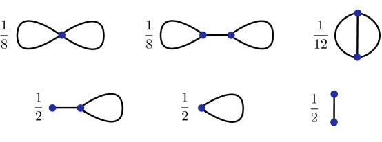
Figure 2. Diagrams contributing to $S_{\gamma,2}$ with symmetry factors. The top row of diagrams have exactly two loops, while the bottom row have fewer loops and additional $1$-vertices and $2$-vertices.

Concretely, the 2-loop contribution from the vacuum energy is

$$\Gamma^{(0)}=\frac{1}{8k}f\mathbf{B}^{-1}\nu-\frac{1}{2}\sum_{s=1}^{k}(\frac{s^{2}}{k^{2}}-\frac{s}{k}+\frac{1}{6})\sum_{i=1}^{N}(1-\zeta^{-m_{i}-s}\theta_{i})^{-1}\,.$$

The four other vertices contribute only at leading order; abbreviating $\tilde{\theta}_{i}=\zeta^{-m_{i}-s}\theta_{i}$ and $\tilde{\theta}_{i}^{\prime}=(1-\zeta^{-m_{i}-s}\theta_{i})^{-1}$, they are

$$\Gamma^{(1)}_{i}=-\frac{1}{2k}(\mathbf{B}^{-1}\nu)_{i}+\frac{1}{k}\sum_{s=1}^{k}\Big{(}\frac{s}{k}-\frac{1}{2}\Big{)}\tilde{\theta}_{i}^{\prime}\,,$$

$$\Gamma^{(2)}_{i}=\frac{1}{k^{2}}\sum_{s=1}^{k}\Big{(}\frac{s}{k}-\frac{1}{2}\Big{)}\tilde{\theta}_{i}\tilde{\theta}_{i}^{\prime}{}^{2}\,,\qquad\Gamma^{(3)}_{i}=-\frac{\tilde{\theta}_{i}\tilde{\theta}_{i}^{\prime 2}}{k\hbar}\,,\qquad\Gamma^{(4)}_{i}=-\frac{\tilde{\theta}_{i}(1+\tilde{\theta}_{i})\tilde{\theta}_{i}^{\prime}{}^{3}}{k\hbar}\,.$$

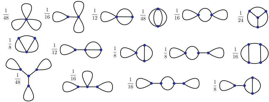
Figure 3. Diagrams with three loops contributing to $S_{3}$.

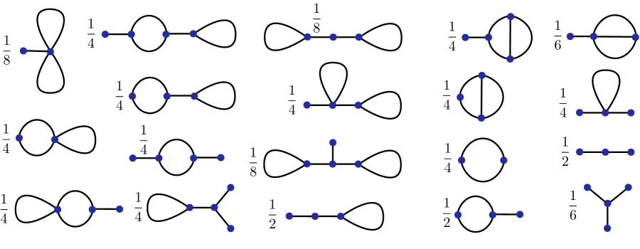
Figure 4. Diagrams with $1$-vertices and $2$-vertices contributing to $S_{3}$.

2.6. The $3$-loop invariant

For the next invariant $S_{\gamma,3,k}$, all the diagrams of Figure 2 contribute, collecting the coefficient of $\hbar^{2}$ of their evaluation. In addition, there are $34$ new diagrams that satisfy the inequality (28); they are shown in Figures 3 and 4. Calculations indicate that the 3-loop invariant $S_{\gamma,3,k}$ is well defined, and invariant under 2-3 moves. The invariants $\tau_{\gamma,k},S_{\gamma,2,k},S_{\gamma,3,k}$ have been programmed in Mathematica as well as in python and take as input a Neumann-Zagier datum readily available from SnapPy [CDW].

The number of diagrams that contribute to the $n$-loop invariant is given in Table 1. For large $n$, we expect that $n!^{2}C^{n}$ diagrams contribute to the $n$-loop invariant. It would be nice to find a more efficient computation.

$n$	$2$	$3$	$4$	$5$	$6$
$g_{n}$	$6$	$40$	$331$	$3700$	$53758$

Table 1. The number $g_{n}$ of graphs that contribute to the $n$-loop invariant for $n=2,\dots,6$.

2.7. Matching with the numerical asymptotics of the Kashaev invariant

Numerical asymptotics of the Kashaev invariant were obtained by Zagier and the second author in [GZ] for several knots, summarized in Table 2. Our $n$-loop invariants at level $k$, presented in Section 5, agree with the numerical computations of [GZ]. This is a strong consistency test for all computational methods.

Knot	Level	Loops
$4_{1}$	$\leq 7$	$\leq 5$
$5_{2}$	$\leq 5$	$\leq 4$
$(-2,3,7)$	$\leq 5$	$\leq 4$
$(-2,3,-3)$	$\leq 3$	$\leq 5$
$(-2,3,9)$	$\leq 3$	$\leq 5$
$6_{1}$	$\leq 3$	$\leq 3$

Table 2. Numerical asymptotics of the Kashaev invariant from [GZ].

2.8. Topological invariance

We conjectured in the introduction that $\phi_{\gamma,\zeta}(\hbar)$ is actually a topological invariant — depending only on a knot $K$ and the root of unity $\zeta$, rather than on a full Neumann-Zagier datum — and thus $\phi_{\gamma,\zeta}(\hbar)=\phi_{K,\zeta}(\hbar)$ is the series that appears in the right hand side of the Quantum Modularity Conjecture. We can now make this a bit more precise.

We begin with the following experimental observations:

• For all 502 hyperbolic knots with at most 8 ideal tetrahedra in the CensusKnots, their default SnapPy triangulations are $\mathbb{Z}$-nondegenerate, in the sense that there is a gauge (for a definition, see Section 2.1) for which $|\!\det\,\mathbf{B}|=1$.

• The default and the canonical SnapPy triangulation of the $5_{2}$ and $6_{1}$ knots have several gauges for which $|\!\det\,\mathbf{B}|=1$. For each of the above knot we have checked that $(\tau_{\gamma,k})^{12k}$ is independent of the above gauges, and that $S_{\gamma,2,k}$ is independent up to addition of $\mathbb{Z}/{24k}$, and that $S_{\gamma,3,k}$ is independent. These are slightly better than the general ambiguities that appear in the nonperturbative level-$k$ state-integral (see Section 4), which motivated the definitions above. Moreover, (local) triangulation-invariance of the level-$k$ state integral suggests that $S_{\gamma,n,k}$ should be independent of triangulation and $\gamma$ for all $n$.

We are therefore led to conjecture

Conjecture 2.9.

For any knot $K$, there exists a triangulation with a non-degenerate Neumann-Zagier datum $\gamma$. The series $\phi_{\gamma,\zeta}(\hbar)$ is independent of the choice of triangulation and $\gamma$, up to multiplication by $\zeta^{\frac{1}{12}}$ and $e^{\hbar/24k}$. Modulo these ambiguities, $\phi_{\gamma,\zeta}(\hbar)=\phi_{K,\zeta}(\hbar)$ equals the series on the right hand side of the Quantum Modularity Conjecture.

Note that if $F_{k}$ does not contain a primitive third root of unity (for example, if $F$ is sufficiently generic and $3\nmid k$) then topological invariance of $(\tau_{k})^{12k}$ together with Theorem 2.2 implies topological invariance of $(\tau_{k})^{4k}$.

3. Proofs

3.1. Proof of Theorem 2.6

First, we need to prove that the summation in Equation (12) is well-defined over the set $(\mathbb{Z}/k\mathbb{Z})^{N}$. This was observed in [GZ] and uses the fact that $\theta^{k}$ is a solution to the Neumann-Zagier equations.

Lemma 3.1.

[GZ] The summation in Equation (12) is $k$-periodic.

Proof.

We need to show that

$$a_{m+ke_{j}}(\theta)=a_{m}(\theta)\,.$$

This follows from the definition of $a_{m}(\theta)$ given in Equation (10), the fact that $z$ is a solution to the Neumann-Zagier equations, and Lemma 3.3 for the cyclic dilogarithm. ∎

To prove Theorem 2.6, recall the Galois extension $F_{G,k}/F_{k}$, and the element $a_{m}(\theta)$ of $F_{G,k}$. Let $\sigma_{j}$ denote the $j$-th generator of the Galois group from Equation (9), and let

(30) $$\epsilon_{j}(\theta)=a_{e_{j}}(\theta)^{-1}\,.$$

The next lemma was observed in [GZ].

Lemma 3.2.

[GZ] For all $m$ we have:

(31) $$\frac{a_{m}(\sigma_{j}\theta)}{a_{m+e_{j}}(\theta)}=\epsilon_{j}(\theta)\,.$$

Proof.

It suffices to show that the left hand side of the above equation is independent of $m$, since the right hand side is the value at $m=0$. To prove this claim, we compute

$$\frac{a_{m}(\sigma_{j}\theta)}{a_{m+e_{j}}(\theta)} =\frac{e^{\pm\pi i\mathbf{B}^{-1}\nu\cdot m}}{e^{\pm\pi i\mathbf{B}^{-1}\nu\cdot(m+e_{j})}}\cdot\frac{\zeta^{\frac{1}{2}\left(m^{T}\mathbf{B}^{-1}\mathbf{A}m\pm\mathbf{B}^{-1}\nu\cdot m\right)}}{\zeta^{\frac{1}{2}\left((m+e_{j})^{T}\mathbf{B}^{-1}\mathbf{A}(m+e_{j})\pm\mathbf{B}^{-1}\nu\cdot(m+e_{j})\right)}}\cdot$$

$$\quad\prod_{i=1}^{N}\frac{(\sigma_{j}\theta_{i})^{-(\mathbf{B}^{-1}\mathbf{A}m)_{i}}}{\theta_{i}^{-(\mathbf{B}^{-1}\mathbf{A}(m+e_{j}))_{i}}}\cdot\prod_{i=1}^{N}\frac{(\zeta\theta_{i}^{-1};\zeta)_{m_{i}+\delta_{i,j}}}{(\zeta\sigma_{j}\theta_{i}^{-1};\zeta)_{m_{i}}}\,.$$

We focus on the $m$-dependent part of each of the 4 fractions. Obviously,

$$\frac{e^{\pm\pi i\mathbf{B}^{-1}\nu\cdot m}}{e^{\pm\pi i\mathbf{B}^{-1}\nu\cdot(m+e_{j})}}=\left(\text{term independent of $m$}\right)\,.$$

Next,

$$\frac{\zeta^{\frac{1}{2}\left(m^{T}\mathbf{B}^{-1}\mathbf{A}m\pm\mathbf{B}^{-1}\nu\cdot m\right)}}{\zeta^{\frac{1}{2}\left((m+e_{j})^{T}\mathbf{B}^{-1}\mathbf{A}(m+e_{j})\pm\mathbf{B}^{-1}\nu\cdot(m+e_{j})\right)}}=\zeta^{-(\mathbf{B}^{-1}\mathbf{A}m)_{j}}\times\left(\text{term independent of $m$}\right).$$

Splitting the product of the third fraction to the case when $j\neq i$ and the case when $j=i$ implies that

$$\prod_{i=1}^{N}\frac{(\sigma_{j}\theta_{i})^{-(\mathbf{B}^{-1}\mathbf{A}m)_{i}}}{\theta_{i}^{-(\mathbf{B}^{-1}\mathbf{A}(m+e_{j}))_{i}}}=\zeta^{(\mathbf{B}^{-1}\mathbf{A}m)_{j}}\times\left(\text{term independent of $m$}\right)\,.$$

Using the identity

$$\frac{(\zeta\theta_{j}^{-1};\zeta)_{m_{j}+1}}{(\zeta^{2}\theta_{j}^{-1};\zeta)_{m_{j}}}=1-\zeta\theta_{j}^{-1}\,,$$

and splitting the product of the fourth fraction to the case when $j\neq i$ and the case when $j=i$ implies that

$$\frac{(\zeta\theta_{i}^{-1};\zeta)_{m_{i}+\delta_{i,j}}}{(\zeta\sigma_{j}\theta_{i}^{-1};\zeta)_{m_{i}}}=\left(\text{term independent of $m$}\right)\,.$$

This completes the proof of the lemma. ∎

Using the fact that the sum is $m$-periodic it follows that

(32) $$\sigma_{j}\left(\sum_{m\in(\mathbb{Z}/k\mathbb{Z})^{N}}a_{m}(\theta)\right)=e_{j}(\theta)\sum_{m\in(\mathbb{Z}/k\mathbb{Z})^{N}}a_{m}(\theta)\,.$$

Suppose that $f(m,\theta)$ is a rational function of $\theta$ with the property that

(33) $$f(m,\sigma_{j}\theta)=f(m+e_{j},\theta)$$

for all $j=1,\dots,N$ and all $m$. Then, it follows that for all $m$ we have

$$a_{m}(\sigma_{j}\theta)f(m,\sigma_{j}\theta)=\epsilon_{j}(\theta)a_{m+e_{j}}(\theta)f(m+e_{j},\theta)\,.$$

Summing up, we obtain that

(34) $$\sigma_{j}\left(\sum_{m\in(\mathbb{Z}/k\mathbb{Z})^{N}}a_{m}(\theta)f(m,\theta)\right)=\epsilon_{j}(\theta)\sum_{m\in(\mathbb{Z}/k\mathbb{Z})^{N}}a_{m}(\theta)f(m,\theta)\,.$$

Equations (32) and (34) and the fact that $F_{G,k}/F_{k}$ is a Galois extension imply that if $f$ satisfies Equation (33), then $\mathrm{Av}(f(-,\theta))\in F_{k}$.

Now observe that the vertex weights of the Feynman diagrams are $\mathbb{Q}(\zeta)$-linear combinations of values of the polylogarithm ${\rm Li}_{l}(\zeta^{m_{i}+s}\theta_{i}^{-1})$ for $l<0$. Since the polylogarithm is a rational function, and $\zeta^{m_{i}}\theta_{i}^{-1}$ satisfies Equation (33) for all $i$ and $j$, Theorem 2.6 follows. ∎

3.2. Some identities of the cyclic dilogarithm

Lemma 3.3.

We have:

(35a) $$D_{k}(\zeta x) =D_{k}(x)\frac{(1-x)^{k}}{1-x^{k}}$$

(35b) $$D^{*}_{k}(\zeta^{-1}x) =D^{*}_{k}(x)\frac{(1-x)^{k}}{1-x^{k}}$$

(35c) $$D_{k}^{*}(x) =\frac{(1-x^{k})^{k-1}}{D_{k}(\zeta x)}$$

(35d) $$D_{k}(x) =e^{\frac{2\pi i}{3}(k^{2}-1)}x^{\frac{k(k-1)}{2}}D^{*}_{k}(1/x)$$

Proof.

Parts (a) and (b) are straightforward. For (35c), use

$$D^{*}_{k}(x)=\prod_{s=1}^{k-1}(1-\zeta^{-s}x)^{s}=\prod_{s=1}^{k-1}(1-\zeta^{s-k}x)^{k-s}=\frac{\left(\prod_{s=1}^{k-1}(1-\zeta^{s}x)\right)^{k}}{\prod_{s=1}^{k-1}(1-\zeta^{s}x)^{s}}=\left(\frac{1-x^{k}}{1-x}\right)^{k}\frac{1}{D_{k}(x)}$$

and then apply (35a). For (35d), use

$$D_{k}(x)=\prod_{s=1}^{k-1}(1-\zeta^{s}x)^{s}=\prod_{s=1}^{k-1}(-\zeta x)^{s}(1-\zeta^{-s}x^{-1})^{s}=e^{\frac{2\pi i}{3}(k^{2}-1)}x^{\frac{k(k-1)}{2}}D^{*}_{k}(1/x)\,.$$

∎

3.3. Proof of Theorem 2.2

Let us define

$$S(\theta) =\sum_{m\in(\mathbb{Z}/k\mathbb{Z})^{N}}a_{m}(\theta)$$

$$P(\theta) =\prod_{i=1}^{N}D_{k}^{*}(\theta_{i}^{-1})^{1/k}\,.$$

To begin with, we have $S(\theta),P^{k}(\theta)\in F_{G,k}$. If $\sigma_{j}$ is the $j$-th generator of the Galois group of $F_{G,k}/F_{k}$ then Equation (32) implies that

$$\sigma_{j}S(\theta)=\epsilon_{j}(\theta)S(\theta)\,.$$

We claim that

(36) $$\sigma_{j}P^{k}(\theta)=\epsilon_{j}(\theta)^{-k}P^{k}(\theta)\,.$$

Combined, they show that $S^{k}(\theta)P^{k}(\theta)\in F_{k}$ which implies Theorem 2.2. To prove Equation (36), we separate the product when $i\neq j$ and when $i=j$ as follows:

$$\frac{\sigma_{j}P^{k}(\theta)}{P^{k}(\theta)} =\left(\prod_{i=1,i\neq j}^{N}\frac{D_{k}^{*}(\sigma_{j}\theta_{i}^{-1})}{D_{k}^{*}(\theta_{i}^{-1})}\right)\cdot\frac{D_{k}^{*}(\sigma_{j}\theta_{j}^{-1})}{D_{k}^{*}(\theta_{j}^{-1})}$$

$$=\frac{D_{k}^{*}(\zeta\theta_{j}^{-1})}{D_{k}^{*}(\theta_{j}^{-1})}$$

$$=\frac{1-z^{-1}_{j}}{(1-\zeta\theta_{j}^{-1})^{k}}\qquad\text{by Equation~{}\eqref{eq.cd2}}\,.$$

On the other hand, $\theta^{k}=z$ satisfies the Neumann-Zagier equations

$$z^{\mathbf{A}}z^{\prime\prime\mathbf{B}}=(-1)^{\nu}$$

Using the fact that $B$ is unimodular, we can write the above equations in the form

$$z^{\prime\prime}=(-1)^{\mathbf{B}^{-1}\nu}z^{-\mathbf{B}^{-1}\mathbf{A}}\,.$$

In other words, for all $j=1,\dots,N$ we have

$$1-z_{j}^{-1}=\prod_{i=1}^{N}z_{i}^{-(\mathbf{B}^{-1}\mathbf{A}e_{j})_{i}}\,.$$

Combining with the above, and the definition of $\epsilon_{j}(\theta)$, concludes the proof of Equation (36). ∎

4. Complex Chern-Simons theory

In this section we review in brief some of the physics of complex Chern-Simons theory, discuss the limits related to the Quantum Modularity Conjecture, and explain how to derive the definition of the series $\phi_{\gamma,\zeta}$ from Section 2.

4.1. Basic structure

Chern-Simons theory with complex gauge group $G_{\mathbb{C}}$ (where $G$ is a compact Lie group) was initially studied by Witten in [Wit89, Wit91]. It is a topological quantum field theory in three-dimensions, whose action is a sum of holomorphic and antiholomorphic copies of the usual Chern-Simons action

(37) $$S(\mathcal{A},\overline{\mathcal{A}})=\frac{t}{8\pi}\,I_{CS}(\mathcal{A})+\frac{\tilde{t}}{8\pi}\,I_{CS}(\overline{\mathcal{A}})\,,$$

where $\mathcal{A}$ is a connection on a $G_{\mathbb{C}}$ bundle over a 3-manifold $M$, and $I_{CS}(\mathcal{A})=\int_{M}(\mathcal{A}d\mathcal{A}+\frac{2}{3}\mathcal{A}^{3})$ (with additional boundary terms if $M$ is not closed). In order for the path-integral measure $\exp(-iS)$ to be invariant under all gauge transformations of $\mathcal{A}$, the levels $t,\tilde{t}$ must obey the quantization condition

(38) $$k:=\tfrac{1}{2}(t+\tilde{t})\in\mathbb{Z}\,.$$

Additionally, the theory is unitary for $\sigma:=\frac{1}{2}(t-\tilde{t})\in i\mathbb{R}$, and less obviously so for $\sigma\in\mathbb{R}$. We will not require unitarity in the following, however.

The classical solutions of Chern-Simons theory are flat $G_{\mathbb{C}}$ connections. Indeed, in the limit $t,\tilde{t}\to\infty$, which corresponds to infinitely weak coupling, the partition function $\mathcal{Z}(t,\tilde{t})=\int D\mathcal{A}\,D\overline{\mathcal{A}}\,e^{-iS}$ is dominated by flat connections

(39) $$\mathcal{Z}(t,\tilde{t}) \sim\sum_{\text{flat $\mathcal{A}^{*}$}}\tau(\mathcal{A}^{*})\exp\bigg{[}\frac{t}{8\pi i}I_{CS}(\mathcal{A}^{*})+\delta(\mathcal{A}^{*})\log t+\sum_{n=2}^{\infty}\bigg{(}\frac{8\pi i}{t}\bigg{)}^{n-1}S_{n}(\mathcal{A}^{*})\bigg{]}$$

$$\hskip 57.81621pt\times\tau(\overline{\mathcal{A}}^{*})\exp\bigg{[}\frac{\tilde{t}}{8\pi i}I_{CS}(\overline{\mathcal{A}}^{*})+\delta(\overline{\mathcal{A}^{*}})\log t+\sum_{n=2}^{\infty}\bigg{(}\frac{8\pi i}{\tilde{t}}\bigg{)}^{n-1}S_{n}(\overline{\mathcal{A}}^{*})\bigg{]}$$

where $\tau(\mathcal{A})^{-2}$ is a Ray-Singer torsion twisted by the flat connection $\mathcal{A}$ and the $S_{n}$ are “higher-loop” topological invariants. For $G_{\mathbb{C}}=SL(2,\mathbb{C})$ and $\mathcal{A}^{*}$ the hyperbolic flat connection, such an asymptotic expansion at weak coupling played a central role in the generalized Volume Conjecture [Guk05].

4.2. A singular limit

At present we are interested in a very different limit in complex Chern-Simons theory, namely $(t,\tilde{t})\to(2k,0)$, or equivalently $\sigma\to k$ with $k\in\mathbb{Z}$ held fixed. This is a singular limit rather than a weak coupling limit. We propose

Conjecture 4.1.

In the limit $(t,\tilde{t})\to(2k,0)$, the partition function of complex Chern-Simons theory has an asymptotic expansion

(40) $$\mathcal{Z}\sim\sum_{\text{flat $\mathcal{A}^{*}$}}\tau_{k}(\mathcal{A}^{*})\exp\bigg{[}\frac{1}{k\hbar}I_{CS}(\mathcal{A}^{*})+\delta(\mathcal{A}^{*})\log(k\hbar)+\sum_{n=2}^{\infty}\hbar^{n-1}S_{n,k}(\mathcal{A}^{*})\bigg{]}\,,$$

where $\hbar=2\pi i\,\tilde{t}/t=2\pi i(\frac{k-\sigma}{k+\sigma})$ and $I_{CS}$ is the holomorphic classical Chern-Simons action. Moreover, if $M=S^{3}\backslash K$ is a hyperbolic knot complement, $G_{\mathbb{C}}=SL(2,\mathbb{C})$, and $\mathcal{A}^{*}$ is the hyperbolic flat connection on $M$, then $\delta(\mathcal{A}^{*})=-\frac{3}{2}$ and the series in the Quantum Modularity Conjecture (2) at $\zeta=e^{2\pi i\alpha}=e^{2\pi i/k}$ is

(41) $$\phi_{K,\zeta}(\hbar)=\tau_{k}(\mathcal{A}^{*})\exp\bigg{[}\sum_{n=2}^{\infty}\hbar^{n-1}S_{n,k}(\mathcal{A}^{*})\bigg{]}\,.$$

Note that, by definition, $I_{CS}(\mathcal{A}^{*})$ already equals the complex hyperbolic volume $V$, so the exponential term $\exp(\frac{1}{k\hbar}V)$ already matches on the right hand side of Equations (40) and (2).

The existence of the expansion (40) is physically far from obvious. One explanation for (40) comes from the so-called 3d-3d correspondence [TY11, DGG14]. An extension of the original correspondence relates Chern-Simons theory at level $k$ on $M$ to the supersymmetric partition function of an associated 3d $\mathcal{N}=2$ theory $T[M]$ on a lens space $L(k,1)\simeq S^{3}/\mathbb{Z}_{k}$ [CJ13, Dim14]. The lens space is a $\mathbb{Z}_{k}$ orbifold of a sphere, whose geometry has been ellipsoidally deformed such that the ratio of minimum to maximum radii is $b=\sqrt{\tilde{t}/t}=\sqrt{\frac{k-\sigma}{k+\sigma}}$. It is well known that as $b\to 0$ the partition function of $T[M]$ on a sphere $L(1,1)\simeq S^{3}$ has an expansion of the form (40), whose leading exponential term is $\frac{1}{\hbar}I_{CS}(\mathcal{A}^{*})$, see [DG13b, TY11, DGG14]. One then expects the $L(k,1)$ partition function to have a similar expansion as $b\to 0$, with leading term $\frac{1}{k\hbar}I_{CS}(\mathcal{A}^{*})$, just as in (40).

There are also some preliminary hints that the existence and structure of (40) may be explained using electric-magnetic duality in four-dimensional Yang-Mills theory, with Chern-Simons theory on its boundary along the lines of [Wit11b, Wit11a]. Indeed, the electric-magnetic duality group $SL(2,\mathbb{Z})$ can relate a singular limit such as $(t,\tilde{t})\to(2k,0)$ to a more standard weak-coupling limit. Electric-magnetic duality has been linked to modular phenomena in the past [VW94], and it is tempting to believe that it could provide a physical basis for Quantum Modularity as well. We aim to explore this further in the future.

4.3. State integrals

Complex Chern-Simons theory has not yet been made mathematically rigorous as a full TQFT, in contrast to Chern-Simons theory with a compact gauge group [Wit89] and the Reshetikhin-Turaev construction [RT91]. Nevertheless, there exist state-integral models, based on ideal triangulations, that provide a definition of complex Chern-Simons partition functions for a certain class of 3-manifolds [Dim14, AK14a]. These state-integral models generalize earlier work [Hik07, DGLZ09, Dim13, AK14b, AK13] that computed Chern-Simons partition functions at level $k=1$.

In the present paper, we use the asymptotic expansion of these state integrals in the limit $(t,\tilde{t})\to(2k,0)$ to motivate the definition of the power series $\phi_{\gamma,\zeta}(\hbar)$ given in Section 2.

Before we discuss the state-integral $\mathcal{Z}_{\gamma}$ associated to a Neumann-Zagier datum $\gamma$ of an ideal triangulation, it is worth mentioning that convergence of the state-integral requires certain positivity assumptions, which are satisfied when the ideal triangulation supports a strict angle structure. This is discussed at length in [AK14a, Dim14]. In the rest of this section, we will assume that the background ideal triangulation admits such a structure. Although positivity is required for the convergence of the state-integral, the formula that we will obtain for its asymptotic expansion makes sense without any positivity assumptions.

It was shown in [Dim13, DG13a] that a Neumann-Zagier datum $\gamma=(\mathbf{A},\mathbf{B},\nu,z,f,f^{\prime\prime})$ with non-degenerate matrix $\mathbf{B}$ leads to a state-integral partition function for $\mathrm{SL}(2,\mathbb{C})$ Chern-Simons at level $k=1$, given by

(42) $$\mathcal{Z}_{\gamma} =\frac{1}{\sqrt{\det\mathbf{B}}}(i)^{f\mathbf{B}^{-1}\nu}e^{\frac{1}{k}(\frac{\hbar}{8}-\frac{\pi^{2}}{8\hbar})f\mathbf{B}^{-1}\nu}\int\frac{d^{N}Z}{(-2\pi i\hbar)^{\frac{N}{2}}}e^{-\frac{1}{2k}(1+\frac{2\pi i}{\hbar})Z\mathbf{B}^{-1}\nu+\frac{1}{2k\hbar}Z\mathbf{B}^{-1}\mathbf{A}Z}\prod_{i=1}^{N}\mathcal{Z}_{\hbar}[\Delta](Z_{i})\,,$$

where the integral runs over some mid-dimensional contour in the space $\mathbb{C}^{N}$ parametrized by $Z=(Z_{1},...,Z_{N})$, and $\mathcal{Z}_{\hbar}[\Delta](Z_{i})$ is a quantum dilogarithm function associated to every tetrahedron, given for $\Re(\hbar)<0$ by

(43) $$\mathcal{Z}_{\hbar}[\Delta](Z_{i})=\prod_{r=0}^{\infty}\frac{1-e^{(r+1)\hbar-Z_{i}}}{1-e^{r\frac{4\pi^{2}}{\hbar})-\frac{2\pi i}{\hbar}Z_{i}}}=\frac{(e^{Z_{i}+\hbar},e^{\hbar})_{\infty}}{(e^{\frac{2\pi i}{\hbar}Z_{i}},e^{\frac{4\pi^{2}}{\hbar}})_{\infty}}\,.$$

This function has an asymptotic expansion as $\hbar\to 0$,

(44) $$\mathcal{Z}_{\hbar}[\Delta](Z_{i}) \sim(e^{Z+\hbar},e^{\hbar})_{\infty}\sim\exp\sum_{n=0}^{\infty}\frac{\hbar^{n-1}}{n!}B_{n}(1){\rm Li}_{2-n}(e^{-Z})$$

$$\hskip 21.68121pt=\frac{1}{\hbar}{\rm Li}_{2}(e^{-Z})+\frac{1}{2}{\rm Li}_{1}(e^{-Z})+\frac{\hbar}{12}{\rm Li}_{0}(e^{-Z})+\ldots\,.$$

Using ${\rm Li}_{2}(e^{-(Z^{*}+\delta Z)})={\rm Li}_{2}(e^{-Z^{*}})+\log(1-e^{-Z^{*}})\delta Z+...$, it follows that at leading order in $\hbar$, the integrand of (42) has critical points at

(45) $$\mathbf{A}Z^{*}+\mathbf{B}\log(1-e^{-Z^{*}})=i\pi\nu\,,$$

which are a logarithmic version of the gluing equations. In particular, if $\gamma$ is a positive Neumann-Zagier datum, then the equations are satisfied by $Z^{*}_{i}=\log(z_{i})$ for all $i=1,\dots,N$. By performing formal Gaussian integration around this “geometric” critical point, order by order in the formal parameter $\hbar$, we obtained in [DG13a] a diagrammatic formula for the series $\phi_{K,1}(\hbar)$.

The actual contour of integration appropriate for (42) and its level-$k$ generalization has been carefully described in [AK14b, Dim14, AK14a]. We emphasize, however, that in order to perform a formal perturbative expansion around a given critical point, a choice of contour is irrelevant.

The level-$k$ generalization of the state integral, as developed in [Dim14], reads

$$\mathcal{Z}_{\gamma}^{(k)} =\frac{1}{k^{N}\sqrt{\det\mathbf{B}}}\zeta^{\frac{1}{4}f\mathbf{B}^{-1}\nu}e^{\frac{1}{k}(\frac{\hbar}{8}-\frac{\pi^{2}}{8\hbar})f\mathbf{B}^{-1}\nu}$$

(46) $$\times\sum_{m\in(\mathbb{Z}/k\mathbb{Z})^{N}}\int\frac{d^{N}Z}{(-2\pi i\hbar)^{\frac{N}{2}}}(-\zeta^{\frac{1}{2}})^{m\mathbf{B}^{-1}\mathbf{A}m}e^{-\frac{1}{2k}(1+\frac{2\pi i}{\hbar})Z\mathbf{B}^{-1}\nu+\frac{1}{2k\hbar}Z\mathbf{B}^{-1}\mathbf{A}Z}\prod_{i=1}^{N}\mathcal{Z}_{\hbar}^{(k)}[\Delta](Z_{i},m_{i})\,,$$

where $\zeta=e^{\frac{2\pi i}{k}}$ as usual, and $(-\zeta^{\frac{1}{2}})^{C}$ is understood as $e^{(\frac{i\pi}{k}-i\pi)C}$ for any $C$; and

(47) $$\mathcal{Z}_{\hbar}^{(k)}[\Delta](Z_{i},m_{i})=\frac{\big{(}\zeta^{m_{i}+1}e^{\frac{\hbar}{k}-\frac{Z_{i}}{k}};\zeta e^{\frac{\hbar}{k}}\big{)}_{\infty}}{\big{(}\zeta^{-m_{i}}e^{-\frac{2\pi i}{k\hbar}{Z_{i}}};\zeta^{-1}e^{\frac{4\pi^{2}}{k\hbar}}\big{)}_{\infty}}\;=\prod_{\mbox{$0\leq s,t<k\atop s-t\,\equiv\,m_{i}\,(\text{mod}\,k)$}}\mathcal{Z}_{\hbar}[\Delta]\Big{(}\frac{Z_{i}}{k}+\hbar\frac{s}{k}+2\pi i\frac{t}{k}\Big{)}\,.$$

Recall some well-known facts about the asymptotic expansion of the quantum dilogarithm that can be found, for instance, in [Zag07, Sec. II.D].

Lemma 4.2.

We have:

$$\log\,(qx;q)_{\infty}=-\sum_{n=1}^{\infty}\frac{q^{n}x^{n}}{n(1-q^{n})}\sim\sum_{n=0}^{\infty}\hbar^{n-1}\frac{(-1)^{n}B_{n}}{n!}{\rm Li}_{2-n}(x)$$

when $q=e^{\hbar}$ and $\hbar\rightarrow 0$, where $B_{n}$ is the $n$-th Bernoulli number and ${\rm Li}_{n}(x)=\sum_{k=1}^{\infty}x^{k}/n^{k}$ is the $n$-th polylogarithm. Since $x\partial_{x}{\rm Li}_{2-n}(x)={\rm Li}_{2-n-1}(x)$, it follows that

$$\log\,(e^{\hbar}e^{-(u+w)};e^{\hbar})_{\infty}\sim\exp\left(\sum_{n,k=0}^{\infty}\hbar^{n-1}\frac{(-1)^{n+k}B_{n}}{n!k!}{\rm Li}_{2-n-k}(e^{-u})w^{k}\right)$$

The asymptotic expansion of $\mathcal{Z}_{\hbar}^{(k)}$ follows from its product representation,

$$\mathcal{Z}_{\hbar}^{(k)}[\Delta](Z_{i},m_{i}) \sim\prod_{s=0}^{k-1}(\zeta^{m_{i}-s}e^{(1-\frac{s}{k})\hbar-\frac{1}{k}Z_{i}};e^{\hbar})_{\infty}$$

(48) $$\sim\exp\sum_{n=0}^{\infty}\sum_{s=1}^{k}\frac{\hbar^{n-1}}{n!}B_{n}\big{(}\tfrac{s}{k}\big{)}{\rm Li}_{2-n}(\zeta^{m_{i}+s}e^{-Z_{i}/k})$$

$$=\exp\bigg{[}\frac{1}{k\,\hbar}{\rm Li}_{2}(e^{-Z_{i}})-\sum_{s=1}^{k}\Big{(}\frac{1}{2}-\frac{s}{k}\Big{)}{\rm Li}_{1}(\zeta^{m_{i}+s}e^{-Z_{i}/k})+\ldots\bigg{]}\,$$

(where we have substituted $s$ by $k-s$ in the second sum). Notably, the leading asymptotic $\frac{1}{k}{\rm Li}_{2}(e^{-Z_{i}})$ is independent of $m_{i}$. Indeed, this remains true for the entire integrand in (46).

The critical points $Z^{*}$ of the integrand at order $\hbar^{-1}$ simply satisfy the standard gluing equation (45). Let us assume that the Neumann-Zagier has all $z_{i}$ strictly in the upper half-plane and focus on the geometric critical point $Z^{*}=\log(z)$. The value of the integrand at the critical point, at order $\hbar^{-1}$, then becomes (after some manipulation)

(49) $$\exp\frac{1}{k\,\hbar}\bigg{[}-\frac{1}{2}(Z^{*}-i\pi f)\cdot((Z^{*})^{\prime\prime}+i\pi f^{\prime\prime})+\sum_{i=1}^{N}{\rm Li}_{2}(e^{-Z_{i}^{*}})\bigg{]}\,,$$

where $(Z^{*})^{\prime\prime}=\log(1-e^{-Z^{*}})=\log z^{\prime\prime}$. The quantity (49) appears to agree with the complex hyperbolic volume of a manifold $M$ with Neumann-Zagier datum $\gamma$, modulo $\pi^{2}/6$ [DG13a], though knowing this is unnecessary for obtaining the series $\phi_{\gamma,\zeta}$. On the other hand, it is crucial for our computation that the value at the leading-order saddle point is independent of $m$ — so all terms in the sum over $m$ contribute equally to the higher-order asymptotics.

By using (4.3), or (better) the double series expansion around the critical point $Z^{*}$,

(50) $$\mathcal{Z}_{\hbar}^{(k)}[\Delta](Z_{i}^{*}+\delta Z_{i},m_{i})\sim\exp\sum_{n=0}^{\infty}\sum_{j=0}^{\infty}\frac{\hbar^{n-1}(-\delta Z_{i})^{j}}{k^{j}\,n!j!}\sum_{s=1}^{k}B_{n}\big{(}\tfrac{s}{k}\big{)}{\rm Li}_{2-n-j}(\zeta^{m_{i}+s}e^{-Z_{i}^{*}/k})\,$$

a saddle-point approximation or formal Gaussian integration of (46) leads immediately to the definition of $\phi_{\gamma,\zeta}(\hbar)$ in Section 2. Indeed, in the finite-dimensional Feynman calculus, the propagator $\Pi$ is the inverse of the Hessian matrix, appearing at order $\hbar^{-1}$ in the exponent of (46) as $\frac{1}{k}\delta Z\cdot(-\mathbf{B}^{-1}\mathbf{A}+\Delta_{(z^{*})^{\prime}})\cdot\delta Z$; while each vertex factor $\Gamma_{i}^{(j)}$ is the coefficient of $(\delta Z_{i})^{j}$ in the exponent of (46).

4.4. Derivation of the torsion

To illustrate how the formal Gaussian integration works, let us derive the $k$-twisted torsion or “1-loop invariant” $\tau_{\gamma,k}$ of (12), starting from (46). Let us set $\zeta=e^{\frac{2\pi i}{k}}$ and $\theta_{i}=z_{i}^{1/k}=e^{Z_{i}^{*}/k}$ as usual, and work at fixed $m\in(\mathbb{Z}/k\mathbb{Z})^{N}$ to start.

There are two contributions to the torsion. First there is the integrand itself, evaluated at $Z=Z^{*}$, keeping only terms of order $\hbar^{0}$ in the exponent:

(51) $$\frac{\zeta^{\frac{1}{4}f\mathbf{B}^{-1}\nu}}{k^{N}(-2\pi i\hbar)^{\frac{N}{2}}\sqrt{\det\mathbf{B}}}\times(-\zeta^{\frac{1}{2}})^{m\mathbf{B}^{-1}\mathbf{A}m}e^{-\frac{1}{2k}Z^{*}\mathbf{B}^{-1}\nu}\prod_{i=1}^{N}\prod_{s=1}^{k}(1-\zeta^{m_{i}+s}e^{-Z_{i}^{*}/k})^{\frac{1}{2}-\frac{s}{k}}\,,$$

where we have used that ${\rm Li}_{1}(x)=-\log(1-x)$. Second, there is the determinant of the Hessian, coming from the leading-order Gaussian integration,

(52) $$\big{[}\det\tfrac{1}{2\pi k\hbar}(-\mathbf{B}^{-1}\mathbf{A}+\Delta_{z})\big{]}^{-\frac{1}{2}}\,.$$

Combining these terms, using $\mathbf{A}f+\mathbf{B}f^{\prime\prime}=\nu$ and $\mathbf{A}Z^{*}+\mathbf{B}(Z^{*})^{\prime\prime}=i\pi\nu$ to rewrite $Z^{*}\mathbf{B}^{-1}\nu$ as $Z^{*}\cdot f^{\prime\prime}-(Z^{*})^{\prime\prime}\cdot f+i\pi f\mathbf{B}^{-1}\nu$, and observing that $\prod_{i=1}^{N}\prod_{s=1}^{k}(1-\zeta^{m_{i}+s}e^{-Z_{i}^{*}/k})^{\frac{1}{2}}=\prod_{i=1}^{N}(1-e^{-Z_{i}^{*}})^{\frac{1}{2}}=(\det\Delta_{z^{\prime\prime}})^{\frac{1}{2}}$, we arrive at

(53) $$\tau_{\gamma,k}=\frac{1}{(ik)^{\frac{N}{2}}\sqrt{\det(\mathbf{A}\Delta_{z}^{\prime\prime}+\mathbf{B}\Delta_{z^{\prime}}^{-1})z^{f^{\prime\prime}/k}z^{\prime\prime}{}^{f/k}}}(-\zeta^{\frac{1}{2}})^{m\mathbf{B}^{-1}\mathbf{A}m}\prod_{i=1}^{N}\prod_{s=0}^{k-1}(1-\zeta^{m_{i}-s}\theta_{i}^{-1})^{s/k}\,.$$

The product may be manipulated further using

$$\prod_{s=0}^{k-1}(1-\zeta^{m_{i}-s}\theta_{i}^{-1})^{\frac{s}{k}}=\prod_{s=-m_{i}}^{k-1-m_{i}}(1-\zeta^{-s}\theta_{i}^{-1})^{\frac{s+m_{i}}{k}}$$

$$\hskip 57.81621pt=z_{i}^{\prime\prime}{}^{\frac{m_{i}}{k}}\prod_{s=k-m_{i}}^{k-1}(1-\zeta^{-s}\theta_{i}^{-1})^{\frac{s}{k}-1}\prod_{s=0}^{k+m_{i}}(1-\zeta^{-s}\theta_{i}^{-1})^{\frac{s}{k}}=z_{i}^{\prime\prime}{}^{\frac{m_{i}}{k}}D_{k}^{*}(\theta_{i}^{-1})^{\frac{1}{k}}(\zeta\theta_{i}^{-1};\zeta)_{m_{i}}^{-1}\,.$$

Finally, setting $\prod_{i}z_{i}^{\prime\prime}{}^{\frac{m_{i}}{k}}=\exp[\frac{1}{k}(Z^{*})^{\prime\prime}\cdot m]=\exp[\frac{i\pi}{k}m\mathbf{B}^{-1}\nu-\frac{1}{k}m\mathbf{B}^{-1}\mathbf{A}Z]=\zeta^{\frac{1}{2}m\mathbf{B}^{-1}\nu}\theta^{-\mathbf{B}^{-1}\mathbf{A}m}$, and summing the whole expression over $m\in(\mathbb{Z}/k\mathbb{Z})^{N}$, we recover (12).

4.5. Ambiguities

The state integral (46) has an intrinsic multiplicative ambiguity [Dim14, Eqn. 5.8]. Namely, it is only defined modulo multiplication by factors (at worst) of the form

(54) $$\big{(}e^{\tfrac{\pi^{2}}{6k\hbar}}\big{)}^{a_{1}}\big{(}\zeta^{\frac{1}{24}}\big{)}^{a_{2}}\big{(}e^{\tfrac{\hbar}{24k}}\big{)}^{a_{3}}\,,\qquad a_{1},a_{2},a_{3}\in\mathbb{Z}\,.$$

The second and third factors affect $\tau_{k}$ and $S_{2,k}$, respectively, in the asymptotic expansion. Higher-order terms in the expansion are unaffected. These ambiguities in the state integral are consistent with those discovered experimentally for $\phi_{\gamma,\zeta}$, as discussed in Section 2.8.

5. Computations

5.1. How the data was computed

We use the Rolfsen notation for knots [Rol90]. SnapPy computes the Neumann-Zagier matrices of default ideal triangulations of the knots below, as well as their exact shapes and trace fields (computed for instance from the Ptolemy module of SnapPy) [GGZ15, CDW].

Given a Neumann-Zagier datum, the 2 and 3-loop invariants at level $k$ are algebraic numbers, elements of the field $F_{K,k}=F_{K}(\zeta_{k})$, where $F_{K}$ is the trace field of $K$ and $\zeta_{k}=e^{\frac{2\pi i}{k}}$. However, these numbers are obtained by sums of algebraic numbers in a much larger number field. Moreover, the 1-loop invariant at level $k$ already contains a $k$-th root of elements of $F_{K,k}$. This makes exact computations impractical. To produce the interesting factorization of Equation (3), and keeping in mind the ambiguities of Section 4.5 we proceed as follows. We know that $x_{k,\ell}=\tau^{k}_{k}/(\tau^{k}_{1}\zeta_{24k}^{\ell})\in F_{K,k}$ for some natural number $\ell$. Given this, we compute the numerical value $x^{\mathrm{num}}_{k,\ell}$ of $x_{k,\ell}$ (for several values of $\ell$) and find a value of $\ell$ for which there is an element $x^{\mathrm{exact}}_{k,\ell}$ of $F_{K,k}$ which is reasonably close to our element. We accomplish this by the LLL algorithm [LLL82]. The Quantum Modularity Conjecture asserts that the exact element of $F_{K,k}$ should to have the form:

(55) $$x^{\mathrm{exact}}_{k,\ell}=\varepsilon_{K,k}\beta_{K,k}^{k}$$

for $\varepsilon_{K,k}\in\mathcal{O}_{F_{K}(\zeta_{k})}^{\times}$ (an algebraic unit) and $\beta_{K,k}\in F_{K}(\zeta_{k})^{\times}$. To find $\epsilon_{K,k}$ and $\beta_{K,k}$, factor the fractional ideal

(56) $$x^{\mathrm{exact}}_{k,\ell}\mathcal{O}_{F_{K}(\zeta_{k})}=\mathfrak{p}_{1}^{e_{1}}\dots\mathfrak{p}_{r}^{e_{r}}$$

into a product of prime ideals $\mathfrak{p}_{i}$, $i=1,\dots,r$. If all ramification exponents $e_{i}$ are divisible by $k$, and if the prime ideals are principal $\mathfrak{p}_{i}=(\wp_{i})$ for $\wp_{i}\in F_{K,k}^{\times}$ (the latter happens when the ideal class group of $F_{K,k}$ is trivial), then we define

$$\beta_{K,k}=\prod_{i=1}^{r}\wp_{i}^{\frac{e_{i}}{k}}\in F_{K,k}^{\times},\qquad\varepsilon_{K,k}=x^{\mathrm{exact}}_{k,\ell}/\beta_{K,k}^{k}\,.$$

It follows that $\varepsilon_{K,k}$ is a unit, and that (55) holds. This gives us strong confidence that $x^{\mathrm{exact}}_{k,\ell}$ is the correct element, and that the computation is correct.

In practice, we have used a Mathematica program to compute $x^{\mathrm{num}}_{k,\ell}$ and $x^{\mathrm{exact}}_{k,\ell}$, and a Sage program (that uses internally pari-gp) to compute the ideal factorization (56).

5.2. A sample computation

Let us illustrate our method of computation in detail with one example, the $5_{2}$ knot with $k=7$. $5_{2}$ is a hyperbolic knot with trace field $F_{5_{2}}=\mathbb{Q}(\alpha)$ where $\alpha=0.8774\dots-0.7448\dots i$ is a root of

$$x^{3}-x^{2}+1=0\,.$$

$F_{5_{2}}$ is of type $[1,1]$ with discriminant $-23$. With the notation of the previous section, and with $\ell=6$, we can numerically compute (with 500 digits of accuracy)

$$x^{\mathrm{num}}_{7,6}=-235162149.63362564574\dots-40898882.99885002594\dots i$$

Fitting with LLL guesses the element of $F_{7}=F(\zeta_{7})$

$$x^{\mathrm{exact}}_{7,6} =-42626237-31168064\alpha+54414583\alpha^{2}+(3905252-48974302\alpha+103510169\alpha^{2})\zeta_{7}+$$

$$(91608760-23650188\alpha+97210659\alpha^{2})\zeta_{7}^{2}+(158817619+22023535\alpha+44886912\alpha^{2})\zeta_{7}^{3}-$$

$$(-149267670-54779388\alpha+17355247\alpha^{2})\zeta_{7}^{4}-(-80916790-45810663\alpha+37182537\alpha^{2})\zeta_{7}^{5}$$

How can we trust this answer? We can compute the norm $N(x^{\mathrm{exact}}_{7,6})$ of $x^{\mathrm{exact}}_{7,6}$ (that is, the product of all Galois conjugates) and find out that:

$$N(x^{\mathrm{exact}}_{7,6})=43^{14}\cdot 6007111235971721^{7}\,.$$

It is encouraging that the above norm is the seventh power of an integer. But even better is the fact that we can factor the ideal generated by the above element as follows:

$$(x^{\mathrm{exact}}_{7,6})=(\wp_{43})^{14}\cdot(\wp_{6007111235971721})^{7}$$

where

$$\wp_{43} =(\alpha-1)\zeta_{7}^{5}+\alpha\zeta_{7}^{2}+\alpha$$

$$\wp_{6007111235971721} =(4\alpha^{2}+6\alpha-7)\zeta_{7}^{5}+(5\alpha^{2}+4\alpha-3)\zeta_{7}^{4}+(8\alpha^{2}+\alpha-8)\zeta_{7}^{3}+$$

$$\quad\,\,(3\alpha^{2}+5\alpha-6)\zeta_{7}^{2}+(2\alpha^{2}+\alpha-5)\zeta_{7}+6\alpha^{2}-2\alpha-2$$

are primes of norm $43$ and $6007111235971721$ (a prime number), respectively. If we define $\beta_{7}=\wp_{43}^{2}\cdot\wp_{6007111235971721}\in F_{7}$ and $\varepsilon_{7}=x^{\mathrm{exact}}_{7,6}/\beta_{7}^{7}$ it follows that

$$x^{\mathrm{exact}}_{7,6}=\varepsilon_{7}\beta_{7}^{7}$$

where $\varepsilon_{7}\in F_{7}^{\times}$ is a unit, given explicitly by the rather long expression:

$$\varepsilon_{7} =(318981244103\alpha^{2}+40488788528803\alpha+30382313828818)\zeta_{7}^{5}+$$

$$\quad\,\,(-52797766935255\alpha^{2}+38212176617858\alpha+58931813581928)\zeta_{7}^{4}+$$

$$\quad\,\,(-29477571352182\alpha^{2}-1263424293533\alpha+15843777055057)\zeta_{7}^{3}+$$

$$\quad\,\,(13260713424737\alpha^{2}+18581482784028\alpha+6470257562608)\zeta_{7}^{2}+$$

$$\quad\,\,(-29079808246903\alpha^{2}+49225269181062\alpha+53729902713340)\zeta_{7}-$$

$$\quad\,\,52974788170701\alpha^{2}+15742594165404\alpha+42070901450997\,.$$

This is an answer that we can trust. There is an additional invariance property of the above unit under the Galois group of $\mathbb{Q}(\zeta_{7})/\mathbb{Q}$, discussed in detail in [CGZ].

6. Data

6.1. The $4_{1}$ knot

The $4_{1}$ knot is the simplest hyperbolic knot with volume $2.0298\dots$ with $2$ ideal tetrahedra and trace field $F_{4_{1}}=\mathbb{Q}(\alpha)=\mathbb{Q}(\sqrt{-3})$ where $\alpha=e^{2\pi i/6}$ is a root of

$$x^{2}-x+1=0\,.$$

$F_{4_{1}}$ is of type $[0,1]$ with discriminant $-3$.

The default SnapPy triangulation of $4_{1}$ generates several Neumann-Zagier data. Most are $\mathbb{Z}$-nondegenerate; for example

(57) $$\gamma\,:\quad\mathbf{A}=\begin{pmatrix}-2&1\\ -1&1\end{pmatrix}\,,\;\;\mathbf{B}=\begin{pmatrix}-1&2\\ -1&1\end{pmatrix}\,,\;\;\nu=(0,0)\,,\;\;z=(\alpha,\alpha)\,,\;\;f=(0,1)\,,\;\;f^{\prime\prime}=(1,0)\,$$

is $\mathbb{Z}$-nondegenerate. The 1-loop invariant at $k=1$ and its norm is given by

(58) $$\begin{array}[]{|c|l|l|}\hline\cr\text{knot}&\tau_{1}^{-2}&N(\tau_{1}^{-2})\\ \hline\cr 4_{1}&2\alpha-1&3\\ \hline\cr\end{array}$$

The norm of the 1-loop of $4_{1}$ at level $k$ is given in (59).

(59) $$\begin{array}[]{|c|l|}\hline\cr k&N(\tau_{k}/\tau_{1})\qquad\text{for $4_{1}$}\\ \hline\cr 1&1\\ \hline\cr 2&3\\ \hline\cr 4&11^{2}\\ \hline\cr 5&3^{4}\cdot 29^{2}\\ \hline\cr 7&39733^{2}\\ \hline\cr 8&3^{4}\cdot 383^{2}\\ \hline\cr 10&19289^{2}\\ \hline\cr 11&3^{10}\cdot 463^{2}\cdot 128237^{2}\\ \hline\cr 13&13339^{2}\cdot 13963^{2}\cdot 130027^{2}\\ \hline\cr 14&3^{6}\cdot 419^{2}\cdot 4451^{2}\\ \hline\cr 16&97^{2}\cdot 418140719^{2}\\ \hline\cr 17&3^{16}\cdot 170239^{2}\cdot 377615549357^{2}\\ \hline\cr 19&571^{2}\cdot 2851^{2}\cdot 27513329^{2}\cdot 83702994059^{2}\\ \hline\cr 20&3^{8}\cdot 59^{2}\cdot 975911939^{2}\\ \hline\cr 22&131^{2}\cdot 14783^{2}\cdot 39667^{2}\cdot 92927^{2}\\ \hline\cr\end{array}$$

In the above table, we avoided the (degenerate) case when $k$ is divisible by $3$, since in those cases the trace field contains the third roots of unity. Notice that the above norms are squares of integers. This exceptional integrality may be a consequence of the fact that $4_{1}$ is amphicheiral.

Next, we give some sample computations of the factorization (3). In this and the next sections, more data has been computed (even for non-prime levels $k$), but only a sample will be presented here. Throughout this section, $\wp_{n}$ will denote a prime in $\mathcal{O}_{F_{k}}$ of norm $n$, a prime power.

For $k=2$ we have

$$\varepsilon_{2} =\alpha$$

$$\beta_{2} =\wp_{3}$$

$$\wp_{3} =2\alpha-1$$

For $k=4$ and $\zeta=\zeta_{4}$ we have

$$\varepsilon_{4} =(-2\alpha+1)\zeta-2$$

$$\beta_{4} =\wp_{11^{2}}$$

$$\wp_{11^{2}} =(-4\alpha+2)\zeta+1$$

For $k=5$ and $\zeta=\zeta_{5}$ we have

$$\varepsilon_{5} =(4\alpha-5)\zeta^{3}+(8\alpha-5)\zeta^{2}+7\alpha\zeta+2\alpha+3$$

$$\beta_{5} =\wp_{3^{3}}\cdot\wp_{29^{2}}$$

$$\wp_{3^{3}} =2\alpha-1$$

$$\wp_{29^{2}} =-2\zeta^{3}+(-\alpha-1)\zeta^{2}-\alpha\zeta+\alpha-2$$

For $k=7$ and $\zeta=\zeta_{7}$ we have

$$\varepsilon_{7} =(60\alpha+115)\zeta^{5}+(239\alpha+90)\zeta^{4}+(390\alpha-61)\zeta^{3}+(415\alpha-240)\zeta^{2}+$$

$$\quad\,\,(300\alpha-300)\zeta+114\alpha-186$$

$$\beta_{7} =\wp_{39733,1}\cdot\wp_{39733,2}$$

$$\wp_{39733,1} =\alpha\zeta^{5}+(\alpha-2)\zeta^{4}+(2\alpha-1)\zeta^{3}+(\alpha-2)\zeta^{2}+(2\alpha-1)\zeta+2\alpha-2$$

$$\wp_{39733,2} =\alpha\zeta^{5}-\zeta^{4}+\alpha\zeta^{3}-\zeta^{2}+(2\alpha-1)\zeta+2\alpha-2$$

For $k=8$ and $\zeta=\zeta_{8}$ we have

$$\varepsilon_{8} =(-12\alpha+36)\zeta^{3}+(17\alpha+17)\zeta^{2}+(36\alpha-12)\zeta+34\alpha-34$$

$$\beta_{8} =\wp_{3^{2},1}\cdot\wp_{3^{2},2}\cdot\wp_{383^{2}}$$

$$\wp_{3^{2},1} =\zeta^{3}-\zeta^{2}-\alpha+1$$

$$\wp_{3^{2},2} =-\zeta^{3}+\alpha\zeta+1$$

$$\wp_{383^{2}} =(-2\alpha+2)\zeta^{3}+(3\alpha-1)\zeta^{2}+(\alpha+1)\zeta-\alpha+3$$

For $k=10$ and $\zeta=\zeta_{10}$ we have

$$\varepsilon_{10} =(-3\alpha+7)\zeta^{3}+(6\alpha-4)\zeta^{2}+(\alpha+1)\zeta+9\alpha-10$$

$$\beta_{10} =\wp_{19289^{2}}$$

$$\wp_{19289^{2}} =(2\alpha-5)\zeta^{3}+(3\alpha+3)\zeta^{2}+(-\alpha+6)\zeta+9\alpha+2$$

For $k=11$ and $\zeta=\zeta_{11}$ we have

$$\varepsilon_{11} =(-353875255116707\alpha+117872583555117)\zeta^{9}+$$

$$\quad\,\,(-688446384174845\alpha+401155759804328)\zeta^{8}+$$

$$\quad\,\,(-897492189704312\alpha+759910737126284)\zeta^{7}+$$

$$\quad\,\,(-914641448990872\alpha+1080237360407592)\zeta^{6}+$$

$$\quad\,\,(-734446808203694\alpha+1260432001194770)\zeta^{5}+$$

$$\quad\,\,(-414120184922386\alpha+1243282741908210)\zeta^{4}+$$

$$\quad\,\,(-55365207600430\alpha+1034236936378743)\zeta^{3}+$$

$$\quad\,\,(227917968648781\alpha+699665807320605)\zeta^{2}+$$

$$\quad\,\,(345790552203898\alpha+345790552203898)\zeta+$$

$$\quad\,\,260826355539896\alpha+84964196664002$$

$$\beta_{11} =\wp_{3^{5},1}\cdot\wp_{3^{5},2}\cdot\wp_{463,1}\cdot\wp_{463,2}\cdot\wp_{128237^{2}}$$

$$\wp_{3^{5},1} =(\alpha-1)\zeta^{8}+(\alpha-1)\zeta^{7}+(\alpha-1)\zeta^{6}+(\alpha-1)\zeta^{5}-\zeta^{4}+(\alpha-1)\zeta^{2}+(\alpha-1)\zeta-1$$

$$\wp_{3^{5},2} =-\zeta^{8}-\alpha\zeta^{5}-\zeta^{4}+(\alpha-1)\zeta^{3}-\zeta+\alpha-1$$

$$\wp_{463,1} =(\alpha-1)\zeta^{9}+\alpha\zeta^{8}+\zeta^{7}-\zeta^{6}+(\alpha-1)\zeta^{5}+\alpha\zeta^{4}+(\alpha-1)\zeta^{2}+\alpha\zeta$$

$$\wp_{463,2} =\alpha\zeta^{8}+\zeta^{7}+\alpha\zeta^{5}+\zeta^{4}+(-\alpha+1)\zeta^{3}+(\alpha-1)\zeta^{2}+\alpha\zeta+1$$

$$\wp_{128237^{2}} =2\alpha\zeta^{9}+2\alpha\zeta^{8}+\zeta^{6}+(-2\alpha+1)\zeta^{5}+(-\alpha-1)\zeta+\alpha-1$$

Some 2 and 3-loop invariants are shown next.

$$\begin{array}[]{|c|l|}\hline\cr k&S_{2,k}\qquad\text{for $4_{1}$}\\ \hline\cr 1&(-10+11\alpha)/108\\ \hline\cr 2&(-25+41\alpha)/216\\ \hline\cr 3&(-20+37\alpha)/108\\ \hline\cr 4&(-977+1855\alpha)/4752+(5\zeta)/44\\ \hline\cr 5&(-14482+37559\alpha)/78300+(11\zeta)/87-(2(-133+11\alpha)\zeta^{2})/2175+((31-22\alpha)\zeta^{3})/2175\\ \hline\cr\end{array}$$

$$\begin{array}[]{|c|l|}\hline\cr k&S_{3,k}\qquad\text{for $4_{1}$}\\ \hline\cr 1&-1/54\\ \hline\cr 2&-19/216\\ \hline\cr 3&-401/1944\\ \hline\cr 4&-17783/52272+347(-1+2\alpha)\zeta/23232\\ \hline\cr 5&(-1569081+48037\alpha)/2838375+48037(-1+2\alpha)\zeta/2838375+\\ &(-64041+64472\alpha)\zeta^{2}/1892250+(-94781-1268\alpha)\zeta^{3}/5676750\\ \hline\cr\end{array}$$

6.2. The $5_{2}$ knot and its partner, the $(-2,3,7)$ pretzel knot

The $5_{2}$ knot is a hyperbolic knot with volume $2.8281\dots$ with $3$ ideal tetrahedra and trace field $F_{5_{2}}=\mathbb{Q}(\alpha)$ where $\alpha=0.8774\dots-0.7448\dots i$ is a root of

$$x^{3}-x^{2}+1=0$$

$F_{5_{2}}$ is of type $[1,1]$ with discriminant $-23$.

The (mirror image of) the $(-2,3,7)$ pretzel knot is a hyperbolic knot same volume and trace field as the $5_{2}$ knot. In fact, the complements of the two knots can be obtained from the same triple of ideal tetrahedra with two different face pairing rules. So, we will use $\alpha$ and $F$ as in Section 6.2. The 1-loop invariant at $k=1$ and its norm is given by

(60) $$\begin{array}[]{|c|l|l|}\hline\cr\text{knot}&\tau_{1}^{-2}&N(\tau_{1}^{-2})\\ \hline\cr 5_{2}&3\alpha-2&-23\\ \hline\cr(-2,3,7)&-6\alpha^{2}+10\alpha-4&-2^{3}\cdot 23\\ \hline\cr\end{array}$$

The norm of the 1-loop of the $5_{2}$ and $(-2,3,7)$ pretzel knots at level $k$ is given in (61) and (62) respectively.

(61) $$\begin{array}[]{|c|l|}\hline\cr k&N(\tau_{k}/\tau_{1})\qquad\text{for $5_{2}$}\\ \hline\cr 1&1\\ \hline\cr 2&11\\ \hline\cr 3&7^{2}\cdot 43\\ \hline\cr 4&21377\\ \hline\cr 5&9491\cdot 1227271\\ \hline\cr 6&709\cdot 2689\\ \hline\cr 7&43^{2}\cdot 6007111235971721\\ \hline\cr 8&17\cdot 113\cdot 7537\cdot 30133993\\ \hline\cr 9&2083098097\cdot 85444190599483\\ \hline\cr 10&1811\cdot 4391\cdot 68626575961\\ \hline\cr 11&363424007\cdot 793250477933\cdot 3103695493140688356241\\ \hline\cr 12&420361\cdot 5976193\cdot 119577001\\ \hline\cr 13&3^{3}\cdot 35023\cdot 17090197144904885763873428788615162336954707155761\\ \hline\cr 14&397951\cdot 4686537997\cdot 36383829926671291\\ \hline\cr 15&61\cdot 271\cdot 5728621\cdot 5533526674625134504126790661929671\\ \hline\cr 16&7^{2}\cdot 17\cdot 6709259559659307953\cdot 10201336785134943810833\\ \hline\cr 17&37251471121483\cdot 478394043550588093915627\cdot\\ &680530260143787862026942663543619843463116564673\\ \hline\cr 18&4519\cdot 8815472623\cdot 178770985453\cdot 2913137889913\\ \hline\cr 19&12772437704449\cdot 3508919046521483041\cdot 498973019420515924143242422019287\cdot\\ &10714512841561797401872096224519192623\\ \hline\cr 20&281\cdot 3821\cdot 3989122481\cdot 3748225906180094225903982496437822401\\ \hline\cr 21&2^{6}\cdot 7^{2}\cdot 211\cdot 337\cdot 913753\cdot 2082346663352803\cdot\\ &17854362817614367334282334028504194189424575574129\\ \hline\cr 22&11\cdot 6029\cdot 54583\cdot 7275369969656838010303\cdot 8746524744220626866965904589334067\\ \hline\cr\end{array}$$

(62) $$\begin{array}[]{|c|l|}\hline\cr k&N(\tau_{k}/\tau_{1})\qquad\text{for $(-2,3,7)$ pretzel}\\ \hline\cr 1&1\\ \hline\cr 2&2\cdot\sqrt{2}\\ \hline\cr 3&373\\ \hline\cr 4&2^{3}\cdot 373\\ \hline\cr 5&7121\cdot 7951\\ \hline\cr 6&2^{3}\cdot 7\cdot 7537\\ \hline\cr 7&38543\cdot 215990584223\\ \hline\cr 8&2^{6}\cdot 47389590553\\ \hline\cr 9&19^{2}\cdot 109\cdot 357859\cdot 3981077803\\ \hline\cr 10&2^{6}\cdot 11^{2}\cdot 971^{2}\cdot 1091\cdot 1151\\ \hline\cr 11&727\cdot 2272057394576817291015189643460557\\ \hline\cr 12&2^{6}\cdot 20467677759464113\\ \hline\cr 13&937\cdot 6761\cdot 160967\cdot 23955361\cdot 635301473\cdot 57335784304171782943\\ \hline\cr 14&2^{9}\cdot 1163\cdot 89392529932786422898277\\ \hline\cr 15&33137687439067819192706277002439756570331\\ \hline\cr 16&2^{12}\cdot 7^{4}\cdot 17\cdot 5963163273069615265031366100433\\ \hline\cr 17&137\cdot 82399986307\cdot 3263165781611\cdot\\ &39270783190888798960324268124076297625100114717631\\ \hline\cr 18&2^{9}\cdot 19\cdot 776332747\cdot 464491149268013810443\\ \hline\cr 19&97553069\cdot 451234687\cdot 4511912067991298785435699217959\cdot\\ &10780714359892164395007021907819650272965937\\ \hline\cr 20&2^{12}\cdot 101\cdot 181^{2}\cdot 58661\cdot 1310381\cdot 311721147290512745903667881\\ \hline\cr 21&2^{6}\cdot 5839\cdot 295429\cdot 10289973200263\cdot 168245809559535775760775546501360397248599028829\\ \hline\cr 22&2^{15}\cdot 8532271651199678660022917719747178676450107088703587421\\ \hline\cr\end{array}$$

Next, we give some sample computations of the factorization (3).

For $k=2$ we have for $5_{2}$

$$\varepsilon_{2} =-\alpha^{2}+\alpha$$

$$\beta_{3} =\wp_{11}$$

$$\wp_{11} =\alpha^{2}+\alpha-2$$

and for $(-2,3,7)$, respectively:

$$\varepsilon_{2} =\alpha+1$$

$$\beta_{2} =\wp_{2^{3}}^{1/2}$$

$$\wp_{2^{3}} =2$$

For $k=3$ and $\zeta=\zeta_{3}$ we have for $5_{2}$

$$\varepsilon_{3} =(-4\alpha^{2}+2\alpha+4)\zeta-4\alpha^{2}-\alpha+1$$

$$\beta_{3} =\wp_{7}^{2}\cdot\wp_{43}$$

$$\wp_{7} =(-\alpha^{2}+1)\zeta-\alpha^{2}+\alpha$$

$$\wp_{43} =2\zeta+\alpha+1$$

and for $(-2,3,7)$, respectively:

$$\varepsilon_{3} =-\alpha^{2}+1$$

$$\beta_{3} =\wp_{373}$$

$$\wp_{373} =(-2\alpha^{2}+2\alpha)\zeta-2\alpha^{2}+\alpha+2$$

For $k=4$ and $\zeta=\zeta_{4}$ we have for $5_{2}$

$$\varepsilon_{4} =-2\alpha\zeta-2\alpha^{2}+\alpha+1$$

$$\beta_{4} =\wp_{21377}$$

$$\wp_{21377} =(4\alpha^{2}-2\alpha+1)\zeta-4\alpha^{2}+2\alpha+2$$

and for $(-2,3,7)$, respectively:

$$\varepsilon_{4} =(2\alpha+2)\zeta+3\alpha^{2}-2$$

$$\beta_{4} =\wp_{2^{3}}\cdot\wp_{373}$$

$$\wp_{2^{3}} =-\zeta+1$$

$$\wp_{373} =(-\alpha^{2}-2\alpha+1)\zeta+\alpha^{2}-\alpha$$

For $k=5$ and $\zeta=\zeta_{5}$ we have for $5_{2}$

$$\varepsilon_{5} =(-\alpha^{2}+3\alpha)\zeta^{3}+(-2\alpha^{2}+\alpha)\zeta^{2}+(2\alpha^{2}-\alpha)\zeta-\alpha^{2}+2\alpha+1$$

$$\beta_{5} =\wp_{9491}\cdot\wp_{1227271}$$

$$\wp_{9491} =(-\alpha^{2}+2)\zeta^{3}+(-\alpha^{2}+\alpha+1)\zeta^{2}+\alpha$$

$$\wp_{1227271} =(2\alpha^{2}+1)\zeta^{3}-\zeta^{2}+(-\alpha^{2}+\alpha)\zeta+1$$

and for $(-2,3,7)$, respectively:

$$\varepsilon_{5} =(-5\alpha-4)\zeta^{3}+(10\alpha^{2}-10\alpha-3)\zeta^{2}+(20\alpha^{2}-10\alpha-2)\zeta+12\alpha^{2}-5\alpha$$

$$\beta_{5} =\wp_{7121}\cdot\wp_{7951}$$

$$\wp_{7121} =(-\alpha^{2}+\alpha-1)\zeta^{3}+(-\alpha^{2}+\alpha-1)\zeta^{2}-\zeta+2\alpha-1$$

$$\wp_{7951} =(\alpha^{2}-\alpha+1)\zeta^{3}+(\alpha+1)\zeta^{2}+(\alpha^{2}-1)\zeta+\alpha^{2}+1$$

For $k=6$ and $\zeta=\zeta_{6}$ we have for $5_{2}$

$$\varepsilon_{6} =(-24\alpha^{2}-12\alpha+4)\zeta-6\alpha^{2}+24\alpha+21$$

$$\beta_{6} =\wp_{709}\cdot\wp_{2689}$$

$$\wp_{709} =(\alpha+1)\zeta-2\alpha^{2}-2$$

$$\wp_{2689} =(\alpha^{2}+2\alpha-3)\zeta-3\alpha^{2}+\alpha+3$$

and for $(-2,3,7)$, respectively:

$$\varepsilon_{6} =(\alpha^{2}-1)\zeta-\alpha^{2}+1$$

$$\beta_{6} =\wp_{2^{6}}^{1/2}\cdot\wp_{7}\cdot\wp_{7357}$$

$$\wp_{2^{6}} =2$$

$$\wp_{7} =(-\alpha^{2}+\alpha+1)\zeta-1$$

$$\wp_{7357} =(-2\alpha^{2}-3\alpha+3)\zeta+2\alpha^{2}+1$$

For $k=7$ and $\zeta=\zeta_{7}$ we have for $5_{2}$

$$\varepsilon_{7} =(318981244103\alpha^{2}+40488788528803\alpha+30382313828818)\zeta^{5}+$$

$$\quad\,\,(-52797766935255\alpha^{2}+38212176617858\alpha+58931813581928)\zeta^{4}+$$

$$\quad\,\,(-29477571352182\alpha^{2}-1263424293533\alpha+15843777055057)\zeta^{3}+$$

$$\quad\,\,(13260713424737\alpha^{2}+18581482784028\alpha+6470257562608)\zeta^{2}+$$

$$\quad\,\,(-29079808246903\alpha^{2}+49225269181062\alpha+53729902713340)\zeta-$$

$$\quad\,\,52974788170701\alpha^{2}+15742594165404\alpha+42070901450997$$

$$\beta_{7} =\wp_{43}^{2}\cdot\wp_{6007111235971721}$$

$$\wp_{43} =(\alpha-1)\zeta^{5}+\alpha\zeta^{2}+\alpha$$

$$\wp_{6007111235971721} =(4\alpha^{2}+6\alpha-7)\zeta^{5}+(5\alpha^{2}+4\alpha-3)\zeta^{4}+(8\alpha^{2}+\alpha-8)\zeta^{3}+$$

$$\quad\,\,(3\alpha^{2}+5\alpha-6)\zeta^{2}+(2\alpha^{2}+\alpha-5)\zeta+6\alpha^{2}-2\alpha-2$$

and for $(-2,3,7)$, respectively:

$$\varepsilon_{7} =(349\alpha^{2}+119\alpha-176)\zeta^{5}+(439\alpha^{2}-196\alpha-450)\zeta^{4}+(60\alpha^{2}-189\alpha-143)\zeta^{3}+$$

$$\quad\,\,(185\alpha^{2}+42\alpha+52)\zeta^{2}+(555\alpha^{2}-154\alpha-278)\zeta+279\alpha^{2}-324\alpha-305$$

$$\beta_{7} =\wp_{38543}\cdot\wp_{215990584223}$$

$$\wp_{38543} =(-\alpha^{2}-\alpha+1)\zeta^{5}+(-\alpha^{2}+1)\zeta^{4}+(-\alpha^{2}-\alpha+1)\zeta^{3}+(-2\alpha+1)\zeta^{2}-\alpha\zeta-\alpha$$

$$\wp_{215990584223} =(-3\alpha^{2}-1)\zeta^{5}+(-5\alpha-3)\zeta^{4}+(2\alpha^{2}-3\alpha-3)\zeta^{3}+$$

$$\quad\,\,(-\alpha^{2}-1)\zeta^{2}+(-3\alpha^{2}-3\alpha+1)\zeta-3\alpha-3$$

For $k=8$ and $\zeta=\zeta_{8}$ we have for $5_{2}$

$$\varepsilon_{8} =(-41580\alpha^{2}+32068\alpha+49052)\zeta^{3}+(-4418\alpha^{2}+43620\alpha+32476)\zeta^{2}+$$

$$\quad\,\,(35332\alpha^{2}+29620\alpha-3124)\zeta+54385\alpha^{2}-1731\alpha-36894$$

$$\beta_{8} =\wp_{17}\cdot\wp_{113}\cdot\wp_{7537}\cdot\wp_{30133993}$$

$$\wp_{17} =\zeta-\alpha^{2}$$

$$\wp_{113} =(\alpha^{2}-\alpha)\zeta^{2}-\zeta+1$$

$$\wp_{7537} =(\alpha-1)\zeta^{3}+(-\alpha^{2}+\alpha)\zeta^{2}+\alpha^{2}\zeta+\alpha$$

$$\wp_{30133993} =(\alpha-1)\zeta^{3}+(-2\alpha^{2}+2\alpha-2)\zeta^{2}+(2\alpha^{2}+2\alpha-1)\zeta$$

and for $(-2,3,7)$, respectively:

$$\varepsilon_{8} =(-245132\alpha^{2}+447868\alpha-364300)\zeta^{3}+(-888194\alpha^{2}+1592676\alpha-1214108)\zeta^{2}+$$

$$\quad\,\,(-1010964\alpha^{2}+1804516\alpha-1352708)\zeta-541525\alpha^{2}+959295\alpha-698910$$

$$\beta_{8} =\wp_{2^{3}}^{2}\cdot\wp_{47389590553}$$

$$\wp_{2^{3}} =\zeta^{3}+1$$

$$\wp_{47389590553} =(-5\alpha^{2}+5\alpha)\zeta^{3}+(4\alpha^{2}-\alpha)\zeta^{2}+(4\alpha^{2}+2\alpha-3)\zeta+\alpha^{2}$$

For $k=9$ and $\zeta=\zeta_{9}$ we have for $5_{2}$

$$\varepsilon_{9} =(-4941\alpha^{2}-5373\alpha)\zeta^{5}+(-12105\alpha^{2}+5373\alpha)\zeta^{4}+(-13605\alpha^{2}+13605\alpha)\zeta^{3}+$$

$$\quad\,\,(-13680\alpha^{2}+10098\alpha)\zeta^{2}+(-11889\alpha^{2}+15471\alpha)\zeta-4535\alpha^{2}+13605\alpha$$

$$\beta_{9} =\wp_{2083098097}\cdot\wp_{85444190599483}$$

$$\wp_{2083098097} =2\alpha^{2}\zeta^{5}+(\alpha^{2}+2)\zeta^{4}+\alpha\zeta^{3}+(\alpha^{2}-1)\zeta^{2}+\alpha^{2}+1$$

$$\wp_{85444190599483} =(3\alpha^{2}-5\alpha+1)\zeta^{5}-\alpha\zeta^{4}+(-2\alpha^{2}-3\alpha+1)\zeta^{3}+(2\alpha^{2}-4\alpha+1)\zeta^{2}+2\alpha^{2}\zeta-4\alpha-1$$

and for $(-2,3,7)$, respectively:

$$\varepsilon_{9} =(331893396\alpha^{2}+165165777\alpha-64446273)\zeta^{5}+$$

$$\quad\,\,(76625316\alpha^{2}+307221984\alpha+188250822)\zeta^{4}+$$

$$\quad\,\,(-214496600\alpha^{2}+305525612\alpha+352863266)\zeta^{3}+$$

$$\quad\,\,(-73359774\alpha^{2}+326036187\alpha+287920791)\zeta^{2}+$$

$$\quad\,\,(-329761962\alpha^{2}+248164137\alpha+375245217)\zeta-$$

$$\quad\,\,431864865\alpha^{2}+54173331\alpha+286988238$$

$$\beta_{9} =\wp_{19^{2}}\cdot\wp_{109}\cdot\wp_{357859}\cdot\wp_{3981077803}$$

$$\wp_{19^{2}} =(-3\alpha^{2}+2)\zeta^{5}+(-2\alpha-2)\zeta^{4}+(3\alpha^{2}-\alpha-3)\zeta^{3}+$$

$$\quad\,\,(-2\alpha^{2}+2\alpha+3)\zeta^{2}+(-3\alpha^{2}+1)\zeta+\alpha^{2}-3\alpha-2$$

$$\wp_{109} =-\alpha^{2}\zeta^{4}-\alpha^{2}\zeta-\alpha^{2}+\alpha$$

$$\wp_{357859} =(-\alpha^{2}+2\alpha)\zeta^{5}+(\alpha^{2}-\alpha-1)\zeta^{4}+(-\alpha^{2}+\alpha+1)\zeta^{3}+$$

$$\quad\,\,(-\alpha^{2}+\alpha)\zeta^{2}+(\alpha^{2}-\alpha-1)\zeta-\alpha^{2}+2$$

$$\wp_{3981077803} =\zeta^{5}+(-2\alpha+2)\zeta^{4}+(\alpha^{2}-\alpha+2)\zeta^{3}+\zeta^{2}+(-\alpha+2)\zeta-\alpha-1$$

For $k=10$ and $\zeta=\zeta_{10}$ we have for $5_{2}$

$$\varepsilon_{10} =(-3824672997\alpha^{2}-3325045215\alpha-330502768)\zeta^{3}+$$

$$\quad\,\,(-2263297486\alpha^{2}+2676462965\alpha+3310113266)\zeta^{2}+$$

$$\quad\,\,(-3762572681\alpha^{2}-400845875\alpha+1841500561)\zeta+$$

$$\quad\,\,100480422\alpha^{2}+4731453922\alpha+3514375210$$

$$\beta_{10} =\wp_{1811}\cdot\wp_{4391}\cdot\wp_{68626575961}$$

$$\wp_{1811} =(\alpha^{2}-\alpha)\zeta^{3}+\alpha^{2}+1$$

$$\wp_{4391} =(-\alpha^{2}+\alpha-1)\zeta^{3}+\zeta^{2}-\alpha^{2}\zeta-\alpha$$

$$\wp_{68626575961} =(-2\alpha^{2}+\alpha+10)\zeta^{3}+(-\alpha^{2}-3\alpha-7)\zeta^{2}+(-\alpha^{2}+2\alpha+5)\zeta+\alpha^{2}-3\alpha-5$$

and for $(-2,3,7)$, respectively:

$$\varepsilon_{10} =(2069226\alpha^{2}-1143696\alpha-2044373)\zeta^{3}+(308318\alpha^{2}+1037807\alpha+609316)\zeta^{2}+$$

$$\quad\,\,(1469403\alpha^{2}-65443\alpha-886914)\zeta-970534\alpha^{2}+1744650\alpha+1872808$$

$$\beta_{10} =\wp_{2^{12}}^{1/2}\cdot\wp_{11^{2}}\cdot\wp_{971^{2}}\cdot\wp_{1091}\cdot\wp_{1151}$$

$$\wp_{2^{6}} =2$$

$$\wp_{11^{2}} =(-\alpha^{2}+\alpha)\zeta^{3}+(-\alpha^{2}+1)\zeta+\alpha^{2}$$

$$\wp_{971^{2}} =\alpha\zeta^{3}+(\alpha^{2}+2)\zeta^{2}+(\alpha^{2}-1)\zeta-\alpha^{2}+\alpha-1$$

$$\wp_{1091} =-\alpha\zeta^{3}+\alpha\zeta-\alpha^{2}+\alpha$$

$$\wp_{1151} =(\alpha^{2}+\alpha-1)\zeta^{2}+(-\alpha^{2}+1)\zeta+\alpha-1$$

Some 2 and 3-loop invariants for $5_{2}$ and $(-2,3,7)$ pretzel knots are shown next.

$$\begin{array}[]{|c|l|}\hline\cr k&S_{2,k}\qquad\text{for $5_{2}$}\\ \hline\cr 1&(245-242\alpha-33\alpha^{2})/2116\\ \hline\cr 2&(6295-10303\alpha-1314\alpha^{2})/46552\\ \hline\cr 3&(1763029-3730884\alpha-616974\alpha^{2})/11464488+(727+40\alpha-52\alpha^{2})\zeta/6923\\ \hline\cr 4&(198755261-468329838\alpha-88322976\alpha^{2})/1085609568-\\ &(-144841-3059\alpha+3724\alpha^{2})\zeta/1966684\\ \hline\cr 5&(1252389600136849-2036921357788788\alpha-291646682299854\alpha^{2})/3697084423961400+\\ &3(109837198792-4170485943\alpha+4920447944\alpha^{2})\zeta/1339523342015+\\ &3(392592030863-20752850276\alpha+41177718597\alpha^{2})\zeta^{2}/6697616710075+\\ &3(-57107525462-19759788121\alpha+42866787232\alpha^{2})\zeta^{3}/6697616710075\\ \hline\cr\end{array}$$

$$\begin{array}[]{|c|l|}\hline\cr k&S_{3,k}\qquad\text{for $5_{2}$}\\ \hline\cr 1&3(18-155\alpha+155\alpha^{2})/24334\\ \hline\cr 2&3(-70769-255956\alpha+319945\alpha^{2})/11777656\\ \hline\cr 3&(-1863760571-9092540536\alpha+10659951670\alpha^{2})/59526487818+\\ &(581674213-725755840\alpha-213728162\alpha^{2})\zeta/29763243909\\ \hline\cr 4&3(-1447363406795-7699225522158\alpha+9371835787629\alpha^{2})/88960456984688-\\ &3(-6173681325057+7935320251722\alpha+1607053670497\alpha^{2})\zeta)/355841827938752\\ \hline\cr 5&3(-10989752660217610311084459-59081913982949711575555062\alpha+\\ &69563350243075727956792969\alpha^{2})/412694240274697972779851750-\\ &3(-4209383365964471973165111+5860219093140674277853192\alpha+\\ &586631030165980383508791\alpha^{2})\zeta/206347120137348986389925875+\\ &9(359260923564919009455273-2046639621559644326769101\alpha+\\ &171017223371634425264447\alpha^{2})\zeta^{2}/412694240274697972779851750+\\ &3(-6713426920522807160021312+3867227919717696039743014\alpha+\\ &2476626379634791382781767\alpha^{2})\zeta^{3}/412694240274697972779851750\\ \hline\cr\end{array}$$

$$\begin{array}[]{|c|l|}\hline\cr k&S_{2,k}\qquad\text{for $(-2,3,7)$ pretzel}\\ \hline\cr 1&(-73-1524\alpha-879\alpha^{2})/25392\\ \hline\cr 2&(5213-6774\alpha+726\alpha^{2})/25392\\ \hline\cr 3&(6428435-7198212\alpha-1601715\alpha^{2})/28413648+(10598-6375\alpha+3506\alpha^{2})\zeta/51474\\ \hline\cr 4&(1772576-2698227\alpha-1231152\alpha^{2})/9471216+(11085-4012\alpha+1543\alpha^{2})\zeta/34316\\ \hline\cr 5&(22745305769203-23958770711676\alpha+1292918125467\alpha^{2})/35941786270800+\\ &(4515992099-1436127126\alpha+641928216\alpha^{2})\zeta/13022386330+\\ &(30141870223-17414407586\alpha+9676608447\alpha^{2})\zeta^{2}/65111931650+\\ &(14370066463-15291381996\alpha+9801845647\alpha^{2})\zeta^{3}/65111931650\\ \hline\cr\end{array}$$

$$\begin{array}[]{|c|l|}\hline\cr k&S_{3,k}\qquad\text{for $(-2,3,7)$ pretzel}\\ \hline\cr 1&(2099-2099\alpha+6874\alpha^{2})/778688\\ \hline\cr 2&(-10438+8532\alpha-177\alpha^{2})/389344\\ \hline\cr 3&(19141449113-148532821745\alpha+206516117210\alpha^{2})/2925128234304+\\ \hline\cr&(7427517757-10156808752\alpha-14120983571\alpha^{2})\zeta/731282058576\\ \hline\cr 4&(181162947-969125569\alpha+2031947518\alpha^{2})/13542260344+\\ \hline\cr&(2348859343-5533235364\alpha+628243915\alpha^{2})\zeta/108338082752\\ \hline\cr 5&(-26527900336733230761869+1135819865279935909813\alpha+\\ &35348426895458618612714\alpha^{2})/312031884139098398776000+\\ &(4131462185677760934998-5937844115855778532936\alpha-\\ &327921124596643988013\alpha^{2})\zeta/78007971034774599694000+\\ &(-3615963624053978498519+2059165800970040528333\alpha-\\ &6722732999448794955676\alpha^{2})\zeta^{2}/78007971034774599694000+\\ &(-7145964286998284204683+6060423272846646989631\alpha\\ &-5019314438337630298992\alpha^{2})\zeta^{3}/78007971034774599694000\\ \hline\cr\end{array}$$

6.3. The $6_{1}$ knot

The $6_{1}$ knot is a hyperbolic knot with volume $3.1639\dots$ with $4$ ideal tetrahedra and trace field $F_{6_{1}}=\mathbb{Q}(\alpha)$ where $\alpha=1.5041\dots-1.2268\dots i$ is a root of

$$x^{4}-2x^{3}+x^{2}+3x+1=0$$

$F_{6_{1}}$ is of type $[0,2]$ with discriminant $257$, a prime. We chose to give the data for this knot because the Bloch group of its trace field is a finitely generated abelian group of rank $2$. The 1-loop invariant at $k=1$ and its norm is given by

(63) $$\begin{array}[]{|c|l|l|}\hline\cr\text{knot}&\tau_{1}^{-2}&N(\tau_{1}^{-2})\\ \hline\cr 6_{1}&7\alpha^{3}-17\alpha^{2}+17\alpha+12&257\\ \hline\cr\end{array}$$

The norm of the 1-loop of $6_{1}$ at level $k$ is given in (64).

(64) $$\begin{array}[]{|c|l|}\hline\cr k&N(\tau_{k}/\tau_{1})\qquad\text{for $6_{1}$}\\ \hline\cr 1&1\\ \hline\cr 2&29\\ \hline\cr 3&79\cdot 373\\ \hline\cr 4&487057\\ \hline\cr 5&401\cdot 8120801581\\ \hline\cr 6&4969\cdot 33601\\ \hline\cr 7&2^{3}\cdot 19013\cdot 3957451\cdot 33546226214089\\ \hline\cr 8&732209\cdot 85423522285273\\ \hline\cr 9&2^{1}2\cdot 19^{2}\cdot 199^{2}\cdot 541\cdot 12313999\cdot 39491789023\\ \hline\cr 10&100981\cdot 317733001\cdot 36502384021\\ \hline\cr 11&291418667\cdot 3515449621583206989038092387793289595509816623\\ \hline\cr 12&157\cdot 15086917\cdot 479105929\cdot 3349280377\\ \hline\cr 13&79\cdot 117777271\cdot 5870910773677\cdot 644682638171983561196398860905544937015222089370889\\ \hline\cr 14&2^{3}\cdot 1405219181759\cdot 57474686640618078167230081699\\ \hline\cr 15&31^{2}\cdot 2379691\cdot 63360261033352141\cdot 1042507380808009331327711940605725261\\ \hline\cr 16&196053041\cdot 21917758321\cdot 2943442798173814595177658255884613139633\\ \hline\cr 18&2^{6}\cdot 19^{2}\cdot 4678492152497445991171\cdot 1135119536120342889490177\\ \hline\cr 20&32261\cdot 500083848464103577816221055593641\cdot 200729720160049090343996502563952161\\ \hline\cr 21&1009\cdot 538727231341573\cdot\\ &69679537903457255216788492238561211259581901781788919921647100909271764443148059688148169\\ \hline\cr 22&23\cdot 1304249\cdot 17520427\cdot 35064943\cdot 662517155967701\cdot 13980312643423978437421727\cdot 653195100488320873699349233\\ \hline\cr\end{array}$$

For $k=2$ we have

$$\varepsilon_{2} =-\alpha^{3}+2\alpha^{2}-\alpha-3$$

$$\beta_{2} =\wp_{29}$$

$$\wp_{29} =-4\alpha^{3}+10\alpha^{2}-8\alpha-7$$

For $k=3$ and $\zeta=\zeta_{3}$ we have

$$\varepsilon_{3} =(-4\alpha^{3}+10\alpha^{2}-9\alpha-8)\zeta-3\alpha^{3}+7\alpha^{2}-5\alpha-8$$

$$\beta_{3} =\wp_{79}\cdot\wp_{373}$$

$$\wp_{79} =(\alpha^{3}-2\alpha^{2}+\alpha+2)\zeta+3\alpha^{3}-7\alpha^{2}+5\alpha+6$$

$$\wp_{373} =(-2\alpha^{3}+5\alpha^{2}-5\alpha-3)\zeta-3\alpha^{3}+7\alpha^{2}-7\alpha-4$$

For $k=4$ and $\zeta=\zeta_{4}$ we have

$$\varepsilon_{4} =(\alpha^{3}-3\alpha^{2}+3\alpha)\zeta+4\alpha^{3}-10\alpha^{2}+8\alpha+10$$

$$\beta_{4} =\wp_{487057}$$

$$\wp_{487057} =(2\alpha^{3}-4\alpha^{2}+2\alpha+4)\zeta+\alpha^{3}-\alpha^{2}+3\alpha-2$$

For $k=5$ and $\zeta=\zeta_{5}$ we have

$$\varepsilon_{5} =(-2\alpha^{2}+6\alpha+24)\zeta^{3}+(-20\alpha^{3}+56\alpha^{2}-38\alpha-12)\zeta^{2}+$$

$$\quad\,\,(-40\alpha^{3}+114\alpha^{2}-92\alpha-68)\zeta-18\alpha^{3}+56\alpha^{2}-49\alpha-40$$

$$\beta_{5} =\wp_{401}\cdot\wp_{8120801581}$$

$$\wp_{401} =(-\alpha^{3}+2\alpha^{2}-\alpha-2)\zeta^{3}+\zeta^{2}+(\alpha^{3}-3\alpha^{2}+3\alpha+2)\zeta$$

$$\wp_{8120801581} =(\alpha+3)\zeta^{3}+(-5\alpha^{3}+11\alpha^{2}-9\alpha-5)\zeta^{2}+(-2\alpha^{3}+3\alpha^{2}-3\alpha-1)\zeta-\alpha^{2}+4$$

For $k=6$ and $\zeta=\zeta_{6}$ we have

$$\varepsilon_{6} =(3\alpha^{3}-8\alpha^{2}+7\alpha+5)\zeta-3\alpha^{3}+7\alpha^{2}-5\alpha-6$$

$$\beta_{6} =\wp_{4969}\cdot\wp_{33601}$$

$$\wp_{4969} =(3\alpha^{3}-7\alpha^{2}+8\alpha+4)\zeta+1$$

$$\wp_{33601} =(4\alpha^{3}-10\alpha^{2}+8\alpha+5)\zeta+\alpha^{3}-3\alpha^{2}+4\alpha+2$$

Some 2 and 3-loop invariants are shown next.

$$\begin{array}[]{|c|l|}\hline\cr k&S_{2,k}\qquad\text{for $6_{1}$}\\ \hline\cr 1&(-178515-946382\alpha+924836\alpha^{2}-371920\alpha^{3})/1585176\\ \hline\cr 2&(-27011582-51129989\alpha+48845639\alpha^{2}-19497370\alpha^{3})/45970104\\ \hline\cr 3&(-82893368809-117384982993\alpha+115430695442\alpha^{2}-47280180216\alpha^{3})/70065571788+\\ &(1706191-1154600\alpha+2708170\alpha^{2}-1385605\alpha^{3})\zeta/22719057\\ \hline\cr 4&(1/3088284268128)(-4950930619209-7026286049126\alpha+7165813225694\alpha^{2}-\\ &2954092842556\alpha^{3})+((84879497-121998463\alpha+149562867\alpha^{2}-\\ &55782966\alpha^{3})\zeta)/500694596\\ \hline\cr 5&-103464360336910543873-188649056185634232247\alpha+173804121553360109686\alpha^{2}-\\ &66971292202517629952\alpha^{3})/64525410081903320700+(2813833153341350-\\ &62305691106986\alpha-557364703389415\alpha^{2}+377823446091675\alpha^{3})\zeta/4184527242665585+\\ &(13304890388975226+6297147216121499\alpha-10590487560881967\alpha^{2}+\\ &4980152420171024\alpha^{3})\zeta^{2}/20922636213327925+(4532417943052961+6683187696077234\alpha-\\ &9628594457667602\alpha^{2}+4438295075710969\alpha^{3})\zeta^{3}/20922636213327925\\ \hline\cr\end{array}$$

$$\begin{array}[]{|c|l|}\hline\cr k&S_{3,k}\qquad\text{for $6_{1}$}\\ \hline\cr 1&(-2772972-2244430\alpha+2833463\alpha^{2}-1140832\alpha^{3})/33949186\\ \hline\cr 2&(-32774690022-17111505319\alpha+26321905652\alpha^{2}-10527251164\alpha^{3})/114205061704\\ \hline\cr 3&(-1598504997001206261-909085206892628307\alpha+1322686345008572948\alpha^{2}-\\ &540917115639525443\alpha^{3})/2387735578783745874+(-340987970089137309-\\ &593382515118577161\alpha+540555632185247860\alpha^{2}-\\ &224218760661580090\alpha^{3})\zeta/2387735578783745874\\ \hline\cr 4&(-76552043703957527182-43852642902836424033\alpha+62680976630422417186\alpha^{2}-\\ &25715623922859379240\alpha^{3})/64428635165146026512-3(40174169918962174465+\\ &74704051006678295591\alpha-69345923760309927344\alpha^{2}+\\ &27498092656227102870\alpha^{3})\zeta/257714540660584106048\\ \hline\cr 5&(-83535030268880547833711035882206548-57630500922078935770505946948391332\alpha+\\ &79407230942955753160123180497661371\alpha^{2}-\\ &30884930225756906416238335746759432\alpha^{3})/45001389388648840291462688518018250+\\ &(-16829652415100927830509785657370971-36833773286121610403780003873363084\alpha+\\ &34528306662808298407142994334953867\alpha^{2}-\\ &13138908536274467739177531307979864\alpha^{3})\zeta/45001389388648840291462688518018250+\\ &(1887348067005309217790728173337463+8201430020783561588938132296311242\alpha-\\ &5410900283083316911728968138281266\alpha^{2}+2484658725916747927696004662854207\alpha^{3})\zeta^{2}/\\ &45001389388648840291462688518018250+(14884459939384051281789536921780086+\\ &35638731679608054276763036584609939\alpha-30236970444383524674457588584916012\alpha^{2}+\\ &12454010292496128569264912949291219\alpha^{3})\zeta^{3}/45001389388648840291462688518018250\\ \hline\cr\end{array}$$

6.4. The $(-2,3,-3)$ and the $(-2,3,9)$ partner pretzel knots

The $(-2,3,9)$ and the mirror of the $(-2,3,-3)$ pretzel knots (the latter is also known as the $8_{20}$ knot) are partners. They can both be assembled from the same set of ideal tetrahedra. It follows that they have equal volume $4.1249\dots$ and equal elements of the Bloch group. They also have equal trace fields $F_{(-2,3,-3)}=F_{(-2,3,9)}=\mathbb{Q}(\alpha)$ where $\alpha=0.4425\dots-0.4544\dots i$ is a root of

$$x^{5}-x^{4}+x^{3}+2x^{2}-2x+1=0$$

This field is of type $[1,2]$ with discriminant $2^{3}\cdot 733$. The 1-loop invariant at $k=1$ and its norm is given by

(65) $$\begin{array}[]{|c|l|l|}\hline\cr\text{knot}&\tau_{1}^{-2}&N(\tau_{1}^{-2})\\ \hline\cr(-2,3,-3)&-10\alpha^{4}+8\alpha^{3}-7\alpha^{2}-22\alpha+13&-2^{4}\cdot 733\\ \hline\cr(-2,3,9)&-4\alpha^{4}+10\alpha^{3}-10\alpha^{2}+2\alpha+14&-2^{7}\cdot 733\\ \hline\cr\end{array}$$

The norm of the 1-loop of the $(-2,3,-3)$ and $(-2,3,9)$ pretzel knots at level $k$ is given in (66) and (67) respectively.

(66) $$\begin{array}[]{|c|l|}\hline\cr k&N(\tau_{k}/\tau_{1})\qquad\text{for $(-2,3,-3)$ pretzel}\\ \hline\cr 1&1\\ \hline\cr 2&9\cdot\sqrt{2}\\ \hline\cr 3&86677\\ \hline\cr 4&2^{2}\cdot 389\cdot 829\\ \hline\cr 5&251\cdot 3701\cdot 5641\cdot 9573881\\ \hline\cr 6&2\cdot 3^{2}\cdot 73\cdot 1675763533\\ \hline\cr 7&21059216779259\cdot 15637926099144015661\\ \hline\cr 8&2^{8}\cdot 1677121\cdot 2821611376969577\\ \hline\cr 9&37\cdot 288361\cdot 16887730311458362485922054098785491\\ \hline\cr 10&2^{2}\cdot 6451\cdot 765151\cdot 2036899317566108665824611\\ \hline\cr 11&572683\cdot 15481222769\cdot 123058773843133908627743611\cdot 40590314050385646643724337053081\\ \hline\cr 12&2^{4}\cdot 7^{2}\cdot 11701\cdot 570178703041\cdot 76017401206533083977\\ \hline\cr 13&3^{3}\cdot 3121\cdot 8581\cdot\\ &5208780692011162885806751823435154606807560938151916182486066554111775765097437387670769\\ \hline\cr 14&2^{3}\cdot 29\cdot 883\cdot 95890797076684070930617\cdot 196704656196706336391779227757264369\\ \hline\cr 15&2731\cdot 84871\cdot 517081\cdot 73175750117941351\cdot 2791635002919906087031\cdot 49318837138663878429931849195141\\ \hline\cr 16&2^{16}\cdot 337\cdot 54673\cdot 55181281\cdot 16869371249354588848817\cdot 2300418425808890616155725510116534231121\\ \hline\cr\end{array}$$

(67) $$\begin{array}[]{|c|l|}\hline\cr k&N(\tau_{k}/\tau_{1})\qquad\text{for $(-2,3,9)$ pretzel}\\ \hline\cr 1&1\\ \hline\cr 2&2^{2}\\ \hline\cr 3&18217\\ \hline\cr 4&2^{5}\cdot 3^{2}\cdot 29\cdot 101\\ \hline\cr 5&31\cdot 28541\cdot 1731399041\\ \hline\cr 6&2^{4}\cdot 31\cdot 11059\cdot 171043\\ \hline\cr 7&43\cdot 197^{2}\cdot 218454864083787040860053\\ \hline\cr 8&2^{1}4\cdot 241\cdot 3361\cdot 1003193\cdot 15946313\\ \hline\cr 9&17594311532167603\cdot 50545284538200619535209\\ \hline\cr 10&2^{8}\cdot 31^{3}\cdot 101\cdot 74098513175515361398321\\ \hline\cr 11&23^{2}\cdot 1917210263\cdot 869440556615693617955386097\cdot 3945088199088552145275994613\\ \hline\cr 12&2^{1}0\cdot 3^{2}\cdot 61\cdot 73\cdot 229\cdot 483950196831635581064375269\\ \hline\cr 13&394369\cdot 1817999\cdot 910838088184909\cdot\\ &1305464531078495668738541122232633072902748130522596602480377557\\ \hline\cr 14&2^{1}2\cdot 23031231430410673\cdot 6254905477428365514627650788018899766459\\ \hline\cr 15&61\cdot 96331\cdot 4470070545691\cdot 144159618930221245901711143825031366430385501494972724861589731\\ \hline\cr 16&2^{2}8\cdot 7^{2}\cdot 764993\cdot 13057776577\cdot 3859919412481173535559894253284600362010320636824481\\ \hline\cr\end{array}$$

Next, we give some sample computations of the factorization (3).

For $k=2$ we have for $(-2,3,-3)$

$$\varepsilon_{2} =\alpha^{3}$$

$$\beta_{3} =\wp_{2}^{1/2}\cdot\wp_{3^{2}}$$

$$\wp_{2} =-\alpha^{4}+\alpha^{3}-\alpha^{2}-2\alpha+1$$

$$\wp_{3^{2}} =\alpha^{3}+\alpha+1$$

and for $(-2,3,9)$, respectively:

$$\varepsilon_{2} =\alpha^{4}-\alpha^{2}+\alpha$$

$$\beta_{2} =\wp_{2^{3}}^{1/2}\cdot\wp_{2}^{1/2}$$

$$\wp_{2^{3}} =\alpha^{4}-\alpha^{3}+3\alpha-2$$

$$\wp_{2} =-\alpha^{4}+\alpha^{3}-\alpha^{2}-2\alpha+1$$

For $k=3$ and $\zeta=\zeta_{3}$ we have for $(-2,3,-3)$

$$\varepsilon_{3} =(\alpha^{4}+\alpha^{2}+2\alpha+1)\zeta+\alpha^{4}+3\alpha-1$$

$$\beta_{3} =\wp_{86677}$$

$$\wp_{86677} =(3\alpha^{4}-\alpha^{3}+8\alpha-1)\zeta+\alpha^{4}+3\alpha$$

and for $(-2,3,9)$, respectively:

$$\varepsilon_{3} =(\alpha^{4}+\alpha^{2}+3\alpha)\zeta+\alpha^{4}-\alpha^{3}+\alpha^{2}+2\alpha-3$$

$$\beta_{3} =\wp_{18217}$$

$$\wp_{18217} =(\alpha^{2}+\alpha+2)\zeta+\alpha^{2}+2$$

For $k=4$ and $\zeta=\zeta_{4}$ we have for $(-2,3,-3)$

$$\varepsilon_{4} =(97/2\alpha^{4}-36\alpha^{3}+55/2\alpha^{2}+211/2\alpha-151/2)\zeta-$$

$$\quad\,\,37/2\alpha^{4}-13\alpha^{3}-15/2\alpha^{2}-107/2\alpha-75/2$$

$$\beta_{4} =\wp_{2}^{2}\cdot\wp_{389}\cdot\wp_{829}$$

$$\wp_{2} =(-1/2\alpha^{4}-1/2\alpha^{2}-1/2\alpha+1/2)\zeta-1/2\alpha^{4}-1/2\alpha^{2}-3/2\alpha+1/2$$

$$\wp_{389} =(-\alpha^{4}+\alpha^{3}-3\alpha+2)\zeta-\alpha^{4}+\alpha^{3}-\alpha^{2}-3\alpha+2$$

$$\wp_{829} =(-3/2\alpha^{4}+\alpha^{3}-3/2\alpha^{2}-7/2\alpha+3/2)\zeta-1/2\alpha^{4}+1/2\alpha^{2}-3/2\alpha+3/2$$

and for $(-2,3,9)$, respectively:

$$\varepsilon_{4} =(-43/2\alpha^{4}+40\alpha^{3}-105/2\alpha^{2}+29/2\alpha+31/2)\zeta+$$

$$\quad\,\,5/2\alpha^{4}+22\alpha^{3}-73/2\alpha^{2}+127/2\alpha-35/2$$

$$\beta_{4} =\wp_{2^{3}}\cdot\wp_{2}^{2}\cdot\wp_{3^{2}}\cdot\wp_{29}\cdot\wp_{101}$$

$$\wp_{2^{3}} =(-1/2\alpha^{4}-1/2\alpha^{2}-3/2\alpha+1/2)\zeta+1/2\alpha^{4}+1/2\alpha^{2}+3/2\alpha-1/2$$

$$\wp_{2} =(-1/2\alpha^{4}-1/2\alpha^{2}-1/2\alpha+1/2)\zeta-1/2\alpha^{4}-1/2\alpha^{2}-3/2\alpha+1/2$$

$$\wp_{3^{2}} =(-1/2\alpha^{4}-1/2\alpha^{2}-3/2\alpha-1/2)\zeta-1/2\alpha^{4}-1/2\alpha^{2}-1/2\alpha+1/2$$

$$\wp_{29} =(\alpha^{4}+\alpha^{2}+2\alpha)\zeta-\alpha$$

$$\wp_{101} =(\alpha^{4}-\alpha^{3}+2\alpha-2)\zeta+\alpha^{4}-\alpha^{3}+\alpha^{2}+2\alpha-2$$

For $k=5$ and $\zeta=\zeta_{5}$ we have for $(-2,3,-3)$

$$\varepsilon_{5} =(6\alpha^{4}+5\alpha^{3}+2\alpha^{2}-2\alpha-9)\zeta^{3}+(-13\alpha^{4}+30\alpha^{3}+9\alpha^{2}-49\alpha+7)\zeta^{2}+$$

$$\quad\,\,(-32\alpha^{4}+30\alpha^{3}+11\alpha^{2}-66\alpha+23)\zeta-31\alpha^{4}+19\alpha^{3}+10\alpha^{2}-48\alpha+25$$

$$\beta_{5} =\wp_{251}\cdot\wp_{3701}\cdot\wp_{5641}\cdot\wp_{9573881}$$

$$\wp_{251} =(\alpha^{4}-\alpha^{3}+\alpha^{2}+2\alpha-1)\zeta^{2}+\alpha\zeta$$

$$\wp_{3701} =(-\alpha^{4}-2\alpha)\zeta^{3}+(\alpha^{4}-\alpha^{3}+\alpha^{2}+2\alpha-2)\zeta^{2}+\alpha$$

$$\wp_{5641} =(\alpha^{3}+\alpha+1)\zeta^{3}+(\alpha^{4}+3\alpha-1)\zeta^{2}+(\alpha^{4}+3\alpha-1)\zeta+\alpha^{4}+3\alpha-1$$

$$\wp_{9573881} =\zeta^{3}+(\alpha^{3}+2)\zeta^{2}+(-\alpha^{4}+\alpha^{3}-2\alpha)\zeta-\alpha^{4}+\alpha^{3}-2\alpha+2$$

and for $(-2,3,9)$, respectively:

$$\varepsilon_{5} =(222\alpha^{4}-1294\alpha^{3}-585\alpha^{2}+990\alpha-662)\zeta^{3}+$$

$$\quad\,\,(1179\alpha^{4}-1708\alpha^{3}-1460\alpha^{2}+1910\alpha-994)\zeta^{2}+$$

$$\quad\,\,(1551\alpha^{4}-677\alpha^{3}-1420\alpha^{2}+1495\alpha-541)\zeta+$$

$$\quad\,\,819\alpha^{4}+379\alpha^{3}-515\alpha^{2}+312\alpha+74$$

$$\beta_{5} =\wp_{31}\cdot\wp_{28541}\cdot\wp_{1731399041}$$

$$\wp_{31} =(-\alpha^{4}+\alpha^{3}-\alpha^{2}-2\alpha+2)\zeta^{3}+(-\alpha^{4}+\alpha^{3}-\alpha^{2}-2\alpha+2)\zeta^{2}+$$

$$\quad\,\,(-\alpha^{4}+\alpha^{3}-\alpha^{2}-2\alpha+1)\zeta-\alpha^{4}+\alpha^{3}-\alpha^{2}-2\alpha+2$$

$$\wp_{28541} =(\alpha^{4}-\alpha^{3}+\alpha^{2}+\alpha-2)\zeta^{3}+(\alpha^{4}+2\alpha)\zeta+2\alpha^{4}-\alpha^{3}+\alpha^{2}+5\alpha-2$$

$$\wp_{1731399041} =-\alpha^{2}\zeta^{3}+(2\alpha^{4}-\alpha^{2}+3\alpha)\zeta^{2}+(3\alpha^{4}+\alpha^{3}-\alpha^{2}+4\alpha)\zeta+3\alpha^{3}-\alpha^{2}-\alpha+3$$

For $k=6$ and $\zeta=\zeta_{6})$ we have for $(-2,3,-3)$

$$\varepsilon_{6} =(20\alpha^{4}-2\alpha^{3}+29\alpha^{2}+21\alpha+35)\zeta-71\alpha^{4}+89\alpha^{3}-144\alpha^{2}-9\alpha+5$$

$$\beta_{6} =\wp_{2^{2}}^{1/2}\cdot\wp_{3^{2}}\cdot\wp_{73}\cdot\wp_{1675763533}$$

$$\wp_{2^{2}} =(-\alpha^{4}+\alpha^{3}-\alpha^{2}-2\alpha+1)\zeta$$

$$\wp_{3^{2}} =\zeta+\alpha^{4}-\alpha^{3}+2\alpha-2$$

$$\wp_{73} =(\alpha^{4}-\alpha^{3}+2\alpha-1)\zeta+\alpha^{4}+2\alpha-1$$

$$\wp_{1675763533} =(-5\alpha^{4}+\alpha^{3}+2\alpha^{2}-10\alpha+3)\zeta+5\alpha^{4}+\alpha^{3}+\alpha^{2}+14\alpha+2$$

and for $(-2,3,9)$, respectively:

$$\varepsilon_{6} =(-30\alpha^{4}+4\alpha^{3}+27\alpha^{2}-21\alpha+5)\zeta+11\alpha^{4}+34\alpha^{3}+\alpha^{2}-17\alpha+14$$

$$\beta_{6} =\wp_{2^{6}}^{1/2}\cdot\wp_{2^{2}}^{1/2}\cdot\wp_{31}\cdot\wp_{11059}\cdot\wp_{171043}$$

$$\wp_{2^{6}} =(\alpha^{4}-\alpha^{3}+3\alpha-2)\zeta-\alpha^{4}+\alpha^{3}-3\alpha+2$$

$$\wp_{2^{2}} =(-\alpha^{4}+\alpha^{3}-\alpha^{2}-2\alpha+1)\zeta$$

$$\wp_{31} =(\alpha+1)\zeta-\alpha$$

$$\wp_{11059} =(-\alpha+2)\zeta+\alpha^{3}-\alpha^{2}+1$$

$$\wp_{171043} =(-2\alpha^{4}+2\alpha^{3}-2\alpha^{2}-3\alpha+2)\zeta+5\alpha^{4}-4\alpha^{3}+3\alpha^{2}+9\alpha-6$$

6.5. The $9_{12}$ knot

The $9_{12}$ knot has volume $8.3664\dots$ with $10$ ideal tetrahedra and trace field $F_{9_{1}2}=\mathbb{Q}(\alpha)$ where $\alpha=-0.06265158\dots+i\,1.24990458\dots$ is a root of

$$x^{17}-8x^{16}+32x^{15}-89x^{14}+195x^{13}-353x^{12}+542x^{11}-719x^{10}+834x^{9}$$

$$\qquad-851x^{8}+764x^{7}-605x^{6}+421x^{5}-253x^{4}+130x^{3}-55x^{2}+18x-3=0$$

$F_{9_{12}}$ is of type $[1,8]$ with discriminant $3\cdot 298171\cdot 5210119\cdot 156953399$. We chose this final example because of the complexity of the ideal triangulation, and the complexity of its trace field. The 1-loop invariant at $k=1$ and its norm is given by

(68) $$\begin{array}[]{|c|l|l|}\hline\cr\text{knot}&\tau_{1}^{-2}&N(\tau_{1}^{-2})\\ \hline\cr 9_{12}&59\alpha^{16}+40\alpha^{15}-14\alpha^{14}+12\alpha^{13}-164\alpha^{12}-82\alpha^{11}+&3\cdot 298171\cdot 5210119\cdot\\ &107\alpha^{10}-186\alpha^{9}-55\alpha^{8}+356\alpha^{7}-387\alpha^{6}-410\alpha^{5}+&156953399\\ &342\alpha^{4}+207\alpha^{3}-117\alpha^{2}-68\alpha-13&\\ \hline\cr\end{array}$$

The norm of the 1-loop of $9_{12}$ at level $k$ is given in (69).

(69) $$\begin{array}[]{|c|l|}\hline\cr k&N(\tau_{k}/\tau_{1})\\ \hline\cr 1&1\\ \hline\cr 2&175013\cdot 139320586381\\ \hline\cr 3&2^{6}\cdot 3\cdot 317089\cdot 618610957\cdot 16597704247\cdot 17781027987117308670607579\\ \hline\cr 4&89^{2}\cdot 193\cdot 113664060425758850100362844843557553491441831726215669353830969\\ \hline\cr\end{array}$$

For $k=2$ and $\zeta=e(1/2)$ we have

$$\varepsilon_{2} =4\alpha^{16}-2\alpha^{13}-8\alpha^{12}-2\alpha^{11}+8\alpha^{10}-13\alpha^{9}+4\alpha^{8}+16\alpha^{7}-24\alpha^{6}-20\alpha^{5}+$$

$$\quad\,\,28\alpha^{4}+12\alpha^{3}-16\alpha^{2}-4\alpha+4$$

$$\beta_{2} =\wp_{175013}\cdot\wp_{139320586381}$$

$$\wp_{175013} =-9\alpha^{16}+12\alpha^{15}-2\alpha^{14}+5\alpha^{13}+15\alpha^{12}-23\alpha^{11}-17\alpha^{10}+50\alpha^{9}-57\alpha^{8}-$$

$$\quad\,\,8\alpha^{7}+98\alpha^{6}-49\alpha^{5}-82\alpha^{4}+52\alpha^{3}+34\alpha^{2}-17\alpha-8$$

$$\wp_{139320586381} =26\alpha^{16}-5\alpha^{15}-4\alpha^{14}-11\alpha^{13}-53\alpha^{12}+2\alpha^{11}+61\alpha^{10}-97\alpha^{9}+42\alpha^{8}+$$

$$\quad\,\,110\alpha^{7}-193\alpha^{6}-94\alpha^{5}+225\alpha^{4}+45\alpha^{3}-124\alpha^{2}-12\alpha+32$$

References

- [AK13] Jørgen Ellegaard Andersen and Rinat Kashaev, A new formulation of the Teichmüller TQFT, 2013, arXiv:1305.4291, Preprint.
- [AK14a] by same author, Complex Quantum Chern-Simons, 2014, arXiv:1409.1208, Preprint.
- [AK14b] by same author, A TQFT from Quantum Teichmüller Theory, Comm. Math. Phys. 330 (2014), no. 3, 887–934.
- [BIZ80] David Bessis, Claude Itzykson, and Jean-Bernard Zuber, Quantum field theory techniques in graphical enumeration, Adv. in Appl. Math. 1 (1980), no. 2, 109–157.
- [CDW] Marc Culler, Nathan M. Dunfield, and Jeffery R. Weeks, SnapPy, http://www.math.uic.edu/t3m/SnapPy.
- [CGZ] Frank Calegari, Stavros Garoufalidis, and Don Zagier, Explicit Chern classes, the quantum Dilogarithm, and the Bloch group, Preprint 2015.
- [CJ13] Clay Cordova and Daniel L. Jafferis, Complex Chern-Simons from M5-branes on the Squashed Three-Sphere, 2013, 1305.2891, Preprint.
- [DG13a] Tudor Dimofte and Stavros Garoufalidis, The quantum content of the gluing equations, Geom. Topol. 17 (2013), no. 3, 1253–1315.
- [DG13b] Tudor Dimofte and Sergei Gukov, Chern-Simons theory and S-duality, J. High Energy Phys. (2013), no. 5, 109, front matter+65.
- [DGG14] Tudor Dimofte, Davide Gaiotto, and Sergei Gukov, Gauge theories labelled by three-manifolds, Comm. Math. Phys. 325 (2014), no. 2, 367–419.
- [DGLZ09] Tudor Dimofte, Sergei Gukov, Jonatan Lenells, and Don Zagier, Exact results for perturbative Chern-Simons theory with complex gauge group, Commun. Number Theory Phys. 3 (2009), no. 2, 363–443.
- [Dim13] Tudor Dimofte, Quantum Riemann surfaces in Chern-Simons theory, Adv. Theor. Math. Phys. 17 (2013), no. 3, 479–599.
- [Dim14] by same author, Complex Chern-Simons theory at level via the 3d-3d correspondence, 2014, arXiv:1409.0857, Preprint.
- [Gar08] Stavros Garoufalidis, Chern-Simons theory, analytic continuation and arithmetic, Acta Math. Vietnam. 33 (2008), no. 3, 335–362.
- [GGZ15] Stavros Garoufalidis, Matthias Goerner, and Christian K. Zickert, The Ptolemy field of 3-manifold representations, Algebr. Geom. Topol. 15 (2015), no. 1, 371–397.
- [GK13] Stavros Garoufalidis and Rinat Kashaev, The -dilogarithm, its state-integrals and their -series, Math. Res. Lett. (2013), arXiv:1304.2705.
- [GK14] by same author, Evaluation of state integrals at rational points, Math. Res. Lett. (2014), arXiv:1411.6062.
- [Guk05] Sergei Gukov, Three-dimensional quantum gravity, Chern-Simons theory, and the A-polynomial, Comm. Math. Phys. 255 (2005), no. 3, 577–627.
- [GZ] Stavros Garoufalidis and Don Zagier, Asymptotics of quantum knot invariants, Preprint 2013.
- [Hik07] Kazuhiro Hikami, Generalized volume conjecture and the -polynomials: the Neumann-Zagier potential function as a classical limit of the partition function, J. Geom. Phys. 57 (2007), no. 9, 1895–1940.
- [Kas95] Rinat M. Kashaev, A link invariant from quantum dilogarithm, Modern Phys. Lett. A 10 (1995), no. 19, 1409–1418.
- [Kas99] by same author, Quantum hyperbolic invariants of knots, Discrete integrable geometry and physics (Vienna, 1996), Oxford Lecture Ser. Math. Appl., vol. 16, Oxford Univ. Press, New York, 1999, pp. 343–359.
- [KMS93] Rinat M. Kashaev, Vladimir V. Mangazeev, and Yu. G. Stroganov, Star-square and tetrahedron equations in the Baxter-Bazhanov model, Internat. J. Modern Phys. A 8 (1993), no. 8, 1399–1409.
- [Lan02] Serge Lang, Algebra, third ed., Graduate Texts in Mathematics, vol. 211, Springer-Verlag, New York, 2002.
- [LLL82] A. K. Lenstra, H. W. Lenstra, Jr., and L. Lovász, Factoring polynomials with rational coefficients, Math. Ann. 261 (1982), no. 4, 515–534.
- [MM01] Hitoshi Murakami and Jun Murakami, The colored Jones polynomials and the simplicial volume of a knot, Acta Math. 186 (2001), no. 1, 85–104.
- [Neu92] Walter D. Neumann, Combinatorics of triangulations and the Chern-Simons invariant for hyperbolic -manifolds, Topology ’90 (Columbus, OH, 1990), Ohio State Univ. Math. Res. Inst. Publ., vol. 1, de Gruyter, Berlin, 1992, pp. 243–271.
- [NZ85] Walter D. Neumann and Don Zagier, Volumes of hyperbolic three-manifolds, Topology 24 (1985), no. 3, 307–332.
- [Rol90] Dale Rolfsen, Knots and links, Mathematics Lecture Series, vol. 7, Publish or Perish Inc., Houston, TX, 1990, Corrected reprint of the 1976 original.
- [RT91] Nikolai Reshetikhin and Vladimir G. Turaev, Invariants of -manifolds via link polynomials and quantum groups, Invent. Math. 103 (1991), no. 3, 547–597.
- [Thu77] William Thurston, The geometry and topology of 3-manifolds, Universitext, Springer-Verlag, Berlin, 1977, Lecture notes, Princeton.
- [TY11] Yuji Terashima and Masahito Yamazaki, Chern-Simons, Liouville, and gauge theory on duality walls, JHEP 1108 (2011), 135, 1103.5748v1.
- [VW94] Cumrun Vafa and Edward Witten, A strong coupling test of -duality, Nuclear Phys. B 431 (1994), no. 1-2, 3–77.
- [Wee05] Jeff Weeks, Computation of hyperbolic structures in knot theory, Handbook of knot theory, Elsevier B. V., Amsterdam, 2005, pp. 461–480.
- [Wit89] Edward Witten, Quantum field theory and the Jones polynomial, Comm. Math. Phys. 121 (1989), no. 3, 351–399.
- [Wit91] by same author, Quantization of Chern-Simons gauge theory with complex gauge group, Comm. Math. Phys. 137 (1991), no. 1, 29–66.
- [Wit11a] by same author, Fivebranes and Knots, 2011, arXiv:1101.3216.
- [Wit11b] by same author, A new look at the path integral of quantum mechanics, Surveys in differential geometry. Volume XV. Perspectives in mathematics and physics, Surv. Differ. Geom., vol. 15, Int. Press, Somerville, MA, 2011, pp. 345–419.
- [Wit89] by same author, -dimensional gravity as an exactly soluble system, Nuclear Phys. B 311 (1988/89), no. 1, 46–78.
- [Zag07] Don Zagier, The dilogarithm function, Frontiers in number theory, physics, and geometry. II, Springer, Berlin, 2007, pp. 3–65.
- [Zag10] by same author, Quantum modular forms, Quanta of maths, Clay Math. Proc., vol. 11, Amer. Math. Soc., Providence, RI, 2010, pp. 659–675.