Rescue of endemic states in interconnected networks with adaptive coupling

Abstract

We study the Susceptible-Infected-Susceptible model of epidemic spreading on two layers of networks interconnected by adaptive links, which are rewired at random to avoid contacts between infected and susceptible nodes at the interlayer. We find that the rewiring reduces the effective connectivity for the transmission of the disease between layers, and may even totally decouple the networks. Weak endemic states, in which the epidemics spreads only if the two layers are interconnected, show a transition from the endemic to the healthy phase when the rewiring overcomes a threshold value that depends on the infection rate, the strength of the coupling and the mean connectivity of the networks. In the strong endemic scenario, in which the epidemics is able to spread on each separate network, the prevalence in each layer decreases when increasing the rewiring, arriving to single network values only in the limit of infinitely fast rewiring. We also find that finite-size effects are amplified by the rewiring, as there is a finite probability that the epidemics stays confined in only one network during its lifetime.

I Introduction

Most biological and sociotecnological systems in nature are not isolated, but they are formed by a set of complex networks which interact following intricate patterns. These systems can be represented in terms of a multilayer network DeDomenico et al. (2013); Kivela et al. (2014) with interconnected layers, in which each network layer describes a different type of connectivity, process, or population. The function of these structures, like sustaining diffusion processes, is characterized by emerging features which are not observed in single-layered systems Domenico et al. (2015); Diakonova et al. (2015a). In particular, epidemics propagating on two interconnected networks show a direct dependence on the patterns of interconnection between the layers. Previous work on the Susceptible-Infected-Susceptible (SIS) model Saumell-Mendiola et al. (2012) showed that interconnected systems can support an endemic state even if each isolated network is not able to do so, and that internetwork correlations boost the propagation on the two-network system. In a related work Dickison et al. (2012) the authors found a mixed phase in the Susceptible-Infected-Recovered (SIR) dynamics –besides the endemic and the healthy phase observed in isolated networks–, in which the epidemics spreads in one network only. The SIR and SIS dynamics on multiplexes was also explored in some recent papers Buono C. and L. (2014); Granell et al. (2014); Sanz et al. (2014).

These and many other works on multilayered systems considered static links inside and between layers, since contacts between individuals are assumed to be constant over time. However, it is known that the frequency and duration of face-to-face contacts are quite heterogeneous, and follow non-trivial patterns Barrat et al. (2004). Past studies in single networks incorporated different mechanisms of time varying topology and network adaptation Holme and Saramaki (2013). A prominent example of time dependent networks are coevolving networks, in which the state of each node is influenced by, and simultaneously shapes, the local network structure Zimmermann et al. (2001, 2004); Gross and Blasius (2008); Gross and Sayama (2009); Vazquez (2013). This coupling of the dynamics on the network with the dynamics of the network leads to a rich variety of different long term behavior of the system. Simple contact processes like the SIS model Gross et al. (2006), the voter model Vazquez et al. (2008); Diakonova et al. (2015b) or the Axelrod model Vazquez et al. (2007) on coevolving networks give rise to new phenomena, not seen in static networks, such as self-organization towards critical behavior, the formation of complex topologies and network fragmentation transitions. Recently, coevolution in mutilayared networks has considered the dynamics of links inside each layer or intralayer links Shai and Dobson (2013); Diakonova et al. (2014), but little attention has been paid to the coevolution of links between layers (interlayer links).

In this paper, we study the SIS model of epidemic spreading on interconnected networks with dynamic connections between layers. Links connecting susceptible and infected individuals at the interlayer are rewired and reconnected to a random pair of susceptible individuals. In this way the dynamics of interlayer links is coupled to the dynamical evolution of the states of the nodes. A related work Shai and Dobson (2013) considered this adaptive mechanism, but only at the level of intra-network connections, keeping interconnections static. We find that the network adaptation process associated with the rewiring of interlayer links can dramatically reduce the spreading of the disease within and between layers. We consider two different scenarios. In weak endemic states, when the epidemics spreads only if the two layers are interconnected, we find a critical rewiring rate beyond which the system remains in the healthy phase. For strong endemic states, in which the epidemics is able to spread on each separate network, we find that rewiring is specially effective in preventing spreading on finite systems. This is so because the link adaptation amplifies finite-size effects, leading to a finite probability that the epidemics stays confined in only one layer during its lifetime.

The paper is organized as follows. In section II, we introduce the model and describe the multilayer topology and the dynamics. In section III, we develop the mathematical framework to study the dynamical properties of the system under two different scenarios, weak endemic states in section IV and strong endemic states in section V. Also, in section V we study the likelihood of transmission between layers in finite systems. We summarize our results and give conclusions in section VI.

II Model description

We study a system of two coupled networks or layers, connected by adaptive interconnections. To build the topology of the system we start from two Erdös-Renyi networks A and B which, for the sake of simplicity, have the same number of nodes $N_{A}=N_{B}=N$ and average degrees $\langle k_{A}\rangle=\langle k_{B}\rangle=\langle k\rangle$. Then, these networks are interconnected with links placed at random between nodes in A and B, whose number remains constant over time, so that the total number of links in the system is conserved. The number of inter-links $q\langle k\rangle N/2$ is proportional to the number of intra-links $\langle k\rangle N/2$ inside each network, where the factor $q\geq 0$ is a measure of the intensity of the coupling, so that for $q=0$ the networks are totally decoupled. As a result, nodes in each network have an average number $\langle k\rangle$ of intranetworks connections and an average number $\langle k_{AB}\rangle=q\langle k\rangle/2$ of internetworks connections.

An SIS epidemics spreads on top of the coupled system, thus each node can be in one of two possible states, either susceptible (state $S$) or infected (state $I$). Each infected node transmits the disease to its susceptible neighbors at some infection rate $\lambda$ ($\lambda_{A}$ and $\lambda_{B}$ inside each layer, and $\lambda_{AB}$ ($\lambda_{BA}$) from nodes in layer A (B) to nodes in layer B (A)), and recovers becoming susceptible again at rate $\mu$, that without loss of generality we take as $\mu=1$. Intralayer links in A and B are fixed in time, but interlayer connections between A and B are allowed to adapt over time. That is, every interconnection between an infected node in network A (B) and a susceptible node in B (A) is randomly rewired at rate a $\omega$. To implement the rewiring, the selected Infected-Susceptible ($IS$) interlink is removed and a new Susceptible-Susceptible ($SS$) interlink is created in its place, in which the susceptible nodes are chosen at random in different layers. In the continuous time version of the model, at every infinitesimal time step $dt$ the processes of infection, recovery and rewiring happen with probabilities $\lambda dt$, $dt$ and $\omega dt$, respectively. We use the Gillespie method Gillespie (2001) to simulate the dynamics. At every iteration step of discrete time length $\Delta t=1/R$, one of the three processes is performed with respective probabilities $\lambda/R$, $1/R$ and $\omega/R$, where $R=\lambda+1+w$ is the total rate.

III Mathematical framework

We develop a mathematical approach in the thermodynamic limit of infinitely large systems, based on a mean-field description at the level of pairs of nodes. This approach allows to study the dynamics of the system in terms of the time evolution of the global densities of nodes and links in the different states. We denote by $I_{A}$ and $S_{A}$ the densities of infected and susceptible nodes in network A, respectively, and by $I_{A}S_{A}$, $I_{A}I_{A}$ and $S_{A}S_{A}$ the densities per node of intranetwork links in A connecting an infected and a susceptible node, two infected nodes and two susceptible nodes, respectively. An analogous notation is used for network B. For interconnections, we use the notation $I_{A}S_{B}$ ($S_{A}I_{B}$) to represent the density per node of internetwork links between an infected node in A (B) and susceptible node in B (A), while $I_{A}I_{B}$ and $S_{A}S_{B}$ stand for the densities of interlinks between two infected nodes and two susceptible nodes, respectively. We note that these quantities are symmetric with respect to the subindices A and B.

Given that the number of nodes in each layer is conserved, as well as the number of intra- and interlinks, the following conservation relations hold at any time:

$$1 = I_{A}+S_{A},$$ (1a)

$$1 = I_{B}+S_{B},$$ (1b)

$$\frac{\left<k_{A}\right>}{2} = S_{A}S_{A}+I_{A}I_{A}+S_{A}I_{A},$$ (1c)

$$\frac{\left<k_{B}\right>}{2} = S_{B}S_{B}+I_{B}I_{B}+S_{B}I_{B},$$ (1d)

$$\left<k_{AB}\right> = S_{A}S_{B}+I_{A}S_{B}+S_{A}I_{B}+I_{A}I_{B}.$$ (1e)

In order to obtain a closed system of equations for the evolution of the densities we make use of the pair approximation (see Appendix A), which assumes that the links of different types are homogeneously distributed over the networks, and thus the densities of triplets can be written in terms of the densities of pairs. We obtain

$$\frac{dI_{A}}{dt} = -I_{A}+\lambda_{A}I_{A}S_{A}+\lambda_{BA}S_{A}I_{B},$$ (2a)

$$\frac{dI_{A}S_{A}}{dt} = 2I_{A}I_{A}-(1+\lambda_{A})I_{A}S_{A}-\lambda_{A}\frac{I_{A}S_{A}\cdot I_{A}S_{A}}{S_{A}}$$ (2b)

$$- \lambda_{BA}\frac{I_{A}S_{A}\cdot S_{A}I_{B}}{S_{A}}+2\lambda_{A}\frac{S_{A}S_{A}\cdot I_{A}S_{A}}{S_{A}}$$

$$+ 2\lambda_{BA}\frac{S_{A}S_{A}\cdot S_{A}I_{B}}{S_{A}},$$

$$\frac{dI_{A}I_{A}}{dt} = -2I_{A}I_{A}+\lambda_{A}I_{A}S_{A}+\lambda_{A}\frac{I_{A}S_{A}\cdot I_{A}S_{A}}{S_{A}}$$ (2c)

$$+ \lambda_{BA}\frac{I_{A}S_{A}\cdot S_{A}I_{B}}{S_{A}},$$

$$\frac{dI_{A}S_{B}}{dt} = I_{A}I_{B}-(1+\omega)I_{A}S_{B}-\lambda_{AB}I_{A}S_{B}$$ (2d)

$$+ \lambda_{A}\frac{I_{A}S_{A}\cdot S_{A}S_{B}}{S_{A}}-\lambda_{B}\frac{I_{B}S_{B}\cdot I_{A}S_{B}}{S_{B}}$$

$$- \lambda_{AB}\frac{I_{A}S_{B}\cdot I_{A}S_{B}}{S_{B}}+\lambda_{BA}\frac{S_{A}I_{B}\cdot S_{A}S_{B}}{S_{A}},$$

$$\frac{dS_{A}I_{B}}{dt} = I_{A}I_{B}-(1+\omega)S_{A}I_{B}-\lambda_{BA}S_{A}I_{B}$$ (2e)

$$+ \lambda_{B}\frac{S_{A}S_{B}\cdot I_{B}S_{B}}{S_{B}}-\lambda_{A}\frac{I_{A}S_{A}\cdot S_{A}I_{B}}{S_{A}}$$

$$- \lambda_{BA}\frac{S_{A}I_{B}\cdot S_{A}I_{B}}{S_{A}}+\lambda_{AB}\frac{I_{A}S_{B}\cdot S_{A}S_{B}}{S_{B}},$$

$$\frac{dI_{A}I_{B}}{dt} = -2I_{A}I_{B}+\lambda_{AB}I_{A}S_{B}+\lambda_{BA}S_{A}I_{B}$$ (2f)

$$+ \lambda_{A}\frac{I_{A}S_{A}\cdot S_{A}I_{B}}{S_{A}}+\lambda_{B}\frac{I_{B}S_{B}\cdot I_{A}S_{B}}{S_{B}}$$

$$+ \lambda_{AB}\frac{I_{A}S_{B}\cdot I_{A}S_{B}}{S_{B}}+\lambda_{BA}\frac{S_{A}I_{B}\cdot S_{A}I_{B}}{S_{A}}.$$

The pair approximation works reasonably well for networks with homogeneous degree distributions and low degree correlations, such as Erdös-Rényi (ER) or degree-regular random graphs, but may not be accurate enough for non-homogeneous or correlated toplogies, like scale-free networks. Even for ER networks, quantitative disagreements between the simulations and the analytical solution may arise in some regimes due to dynamic correlations not captured by the approximation, as it happens when the system is close to the healthy absorbing state Demirel et al. (2014).

The set of non-linear coupled ordinary differential Eqs. (2) together with the conservation laws Eqs. (1) form a closed set of equations for the system’s dynamics. This mathematical framework is suitable to study macroscopic quantities, such as the prevalence of the epidemics (stationary density of infected nodes $I_{A}$ and $I_{B}$) in each layer. We are particularly interested in the effects of the rewiring on the prevalence, thus we focus on the dependence of $I_{A}$ and $I_{B}$ on the rewiring rate $\omega$. We shall see that the behavior of the coupled system at the stationary state differs qualitatively depending on whether the global endemic state is weak or strong, with strong endemic states having the capacity to propagate on each network separately, while weak endemic states are unable to do so Saumell-Mendiola et al. (2012). We recall that strong endemic states are supported by infectivity levels above the critical value $\lambda_{c}$ in each single layer, while weak endemic states appear whenever the infectivity is below the single epidemic threshold $\lambda_{c}$, but above the epidemic threshold $\lambda_{c,q}$ of the interconnected system, which depends on the coupling $q$. In single random uncorrelated networks the critical threshold is typically given by the expression $\lambda_{c}=\left<k\right>/\left<k^{2}\right>$ Pastor-Satorras and Vespignani (2001), and it can be better approximated by $\lambda_{c}=\left<k\right>/\left<k(k-1)\right>$ Saumell-Mendiola et al. (2012), which corrects in part the effect of dynamical correlations. In ER networks $\left<k^{2}\right>=\left<k\right>^{2}+\left<k\right>$, and thus the single-layer threshold is reduced to the simple expression Luo et al. (2014)

$$\lambda_{c}=\frac{1}{\left<k\right>}.$$ (3)

IV Weak endemic states

As we mentioned above, the existence of endemic states in the coupled system of two layers is possible even when infection rates are below the critical rate $\lambda_{c}$ of a single layer, as was shown in Saumell-Mendiola et al. (2012). It turns out that the infection in each layer is reinforced by its partner layer through the interconnections, and thus the entire system lowers its epidemic threshold to a new value $\lambda_{c,q}<\lambda_{c}$, associated to the interconnectivity $q$. Therefore, endemic sates are also observed for infection rates in the region $\lambda_{c,q}\leq\lambda\leq\lambda_{c}$. In this section we focus on the $\lambda<\lambda_{c}$ case, and analyze separately the case scenarios of static and dynamic interconnections.

IV.1 Static interlayer links

For the sake of simplicity, we consider the symmetric case $\lambda_{A}=\lambda_{B}=\lambda_{AB}=\lambda_{BA}=\lambda<\lambda_{c}$. According to the general heterogeneous mean-field approach in Saumell-Mendiola et al. (2012), the epidemics can propagate on a system of two identical networks whenever the dynamical and topological characteristic parameters fulfill the condition

$$\alpha>(1-\Lambda)(1-\Omega).$$ (4)

Here $\Lambda=\lambda\left<k^{2}\right>/\left<k\right>$ is the maximum eigenvalue of the characteristic matrix of each single network, which determines the condition for the existence of an endemic state whenever $\Lambda>1$. We next particularize for the case of ER networks. Taking into account the partial correction for the effect of dynamical correlations Saumell-Mendiola et al. (2012), the maximum eigenvalue for an isolated ER network is $\Lambda=\lambda\left<k(k-1)\right>/\left<k\right>=\lambda\left<k\right>$. The factor $\Omega=\lambda\left<k^{2}_{AB}\right>/\left<k_{AB}\right>$ is the counterpart for the bipartite network of interconnections, whose first and second degree moments are $\left<k_{AB}\right>$ and $\left<k_{AB}^{2}\right>=\left<k_{AB}\right>\left(\left<k_{AB}\right>+1\right)$ and hence $\Omega=\lambda\left(\left<k_{AB}\right>+1\right)$. Finally, the factor $\alpha$ given by $\lambda^{2}\left<k\cdot k_{AB}\right>^{2}/\left<k\right>\left<k_{AB}\right>$ can be approximated as $\alpha\simeq\lambda^{2}\left<k\right>\left<k_{AB}\right>$. Plugging the values for $\Lambda$, $\Omega$ and $\alpha$ into Eq. (4) we arrive to the condition

$$(\lambda-\lambda_{c,q,+})(\lambda-\lambda_{c,q,-})<0,$$ (5)

with

$$\lambda_{c,q,\pm}=\frac{1+(1+\frac{q}{2})\left<k\right>\pm\sqrt{\left[1+(1+\frac{q}{2})\left<k\right>\right]^{2}-4\left<k\right>}}{2\left<k\right>}.$$

(6)

Infection rates in the range $\lambda_{c,q,-}<\lambda<\min(\lambda_{c,q,+},\lambda_{c})$ fulfill the condition Eq. (5), and thus they are able to spread the epidemics on the coupled system, even if $\lambda$ is below the single network threshold $\lambda_{c}=1/\left<k\right>$. Even though Eq. (6) gives a good estimation of the infection threshold, a more precise expression for $\lambda_{c,q}$ can be obtained using the homogeneous pair approximation of section III [from Eqs. (1) and (2)]. The limit for $\omega=0$ of the general result reported in section IV.2 is

$$\lambda_{c,q}=\frac{1}{(1+q/2)\left<k\right>},$$ (7)

which reduces to Eq. (3) in the absence of coupling $q=0$. This result correspond to the value of the critical infection rate for a single layer ER network with average degree $\left<k\right>+\left<k_{AB}\right>=(1+q/2)\left<k\right>$. Critical infection rates from Eq. (6) and Eq. (7) turn out to be numerically very similar [see Fig. (1)].

Figure 1: Critical infection rate $\lambda_{c,q}^{\omega}$ of a system of two interconnected networks of average degree $\left<k\right>=4$ vs the coupling factor $q$. Solid lines represent the expression Eq. (15) for different values of the rewiring rate $\omega=\infty,16,4,1$ and $0$ (from top to bottom), while the dashed line is the approximation from Eq. (6) for $\omega=0$

.

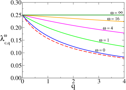
IV.2 Adaptive interlayer links

Next, we study the behavior of the system when interconnections are rewired at a given rate $\omega$ to avoid contacts between infected and susceptible nodes at the interlayer.

Figure 2: Disease prevalence $I_{A}=I_{B}$ in a symmetric two-network system as a function of the rewiring rate $\omega$. Each network has average degree $\left<k\right>=4$. Circles are the results from the numerical integration of Eqs. (2), while lines are the analytical approximation Eq. (28). (a) For infection rate $\lambda=0.23$ and values of the coupling $q=0.7,0.6,0.5,0.4,0.3$ and $0.2$ (from top to bottom). (b) For $q=0.5$ and values of the infection rate $\lambda=0.26,0.25,0.24,0.23,0.22$ and $0.21$ (top to bottom).

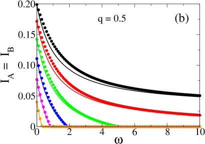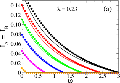
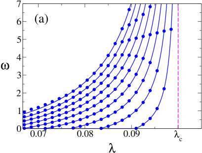
In Fig. 2 we show the prevalence $I_{A}=I_{B}$ in networks A and B for a symmetric system with $\left<k\right>=4$, as predicted by the analytic Eqs. (2) (solid circles). We show as well the approximate analytic solution of Eqs. (2) (solid lines) that we derive in Appendix B. We observe that the prevalence decreases as the rewiring increases, and vanishes at a finite value $\omega_{c,q}^{\lambda}$ when $\lambda<\lambda_{c}=1/\left<k\right>=0.25$. That is, there is a continuous transition from an endemic to a healthy phase when the rewiring overcomes a critical value $\omega_{c,q}^{\lambda}$, which depends on the coupling $q$ and the infection rate $\lambda<0.25$. In Fig. 3(a) we plot the critical rewiring rate vs the infectivity $\lambda$ for various values of $q$ and $\left<k\right>=10$, obtained from the numerical integration of Eqs. (2) (dots). As we can see, $\omega_{c,q}^{\lambda}$ is larger for larger values of $q$ and $\lambda$, and diverges as $\lambda$ approaches $\lambda_{c}=1/\left<k\right>=0.1$. This divergence means that for strong endemic states ($\lambda>0.1$) there is no finite rewiring able to stop the spreading. In the next section, we explore this phenomenon in more detail.

Figure 3: (a) Critical rewiring rate $\omega_{c,q}^{\lambda}$ vs infectivity $\lambda$ for a symmetric two-network system with average degree $\left<k\right>=10$, obtained from Eqs. (2) (dots) and from Eq. (12) (solid lines), for values of the coupling $q=0.2,0.4,0.6,0.8,1.0,1.2,1.4,1.6$ and $1.8$ (from left to right). (b) Healthy-endemic phase diagram for two coupled ER networks of $N=10^{4}$ nodes each, average degree $\left<k\right>=10$, and coupling $q=1.0$. One-layer and two-layer critical infection rates are $\lambda_{c}=0.1$ and $\lambda_{c,q}=0.067$, respectively. Filled circles are results from simulations, while the solid line is the analytical solution Eq. (12) of the system of Eqs. (2).

We now derive an analytical expression for the dependence of the critical rewiring with the infectivity $\lambda$ and the average connectivities $\left<k\right>$ and $q$. To that end, we use the system of Eqs. (2) to study the stability of the healthy phase under a small perturbation that consists on infecting a small fraction of nodes in both layers. For simplicity, we consider the symmetric case scenario in which both perturbations are the same, so that initially $I_{A}=I_{B}\ll 1$. Because of the symmetries of the system and initial conditions, the prevalence in both networks must be the same, thus $I_{B}S_{B}=I_{A}S_{A}$, $I_{B}I_{B}=I_{A}I_{A}$ and $S_{A}I_{B}=I_{A}S_{B}$. This reduces Eqs. (2) to a system of five equations with five unknown densities: $I_{A},I_{A}S_{A},I_{A}I_{A},I_{A}S_{B}$ and $I_{A}I_{B}$. Given that these densities depend on the number of infected nodes and $I_{A}\ll 1$, they are also very small initially. Then, we linearize the equations around the fixed point $S_{A}=S_{B}=1,S_{A}S_{A}=S_{B}S_{B}=\langle k\rangle/2,S_{A}S_{B}=\langle k_{AB}\rangle=q\langle k\rangle/2$, by neglecting terms of order $2$ or higher in the five densities. We obtain a reduced system which can be written in matrix representation as

$$\frac{d{\bf I}}{dt}={\bf AI},$$ (8)

where

$${\bf A}\equiv\left(\begin{array}[]{ccccc}-1&\lambda&0&\lambda&0\\ 0&\lambda\langle k\rangle-\lambda-1&2&\lambda\langle k\rangle&0\\ 0&\lambda&-2&0&0\\ 0&\lambda\langle k\rangle&0&\frac{q}{2}\lambda\langle k\rangle-\lambda-1-w&1\\ 0&0&0&2\lambda&-2\end{array}\right),$$

and

$${\bf I}\equiv\left(\begin{array}[]{ccccc}I_{A}&I_{A}S_{A}&I_{A}I_{A}&I_{A}S_{B}&I_{A}I_{B}\end{array}\right).$$

At the critical point, the determinant of $\bf A$ must be zero, from where

$$\left(\lambda\langle k\rangle-1\right)\left[q\lambda\langle k\rangle-2(1+w)\right]-q\lambda^{2}\langle k\rangle^{2}=0.$$ (11)

Finally, solving for $\omega$ we obtain the critical rewiring rate

$$\omega_{c,q}^{\lambda}=\frac{(1+q/2)\lambda\langle k\rangle-1}{1-\lambda\langle k\rangle}.$$ (12)

All real parts of the eigenvalues of the Jacobian matrix ${\bf A}$ must be strictly negative for the healthy state solution ${\bf I=0}$ to be stable. Then, a sufficient condition for the instability is the existence of a positive real part of one of the five eigenvalues. This happens in two regions $R_{1}$ and $R_{2}$ of the $\omega-\lambda$ phase space that fulfill the conditions

$$\lambda>\lambda_{c}~{}~{} ~{}~{}\omega\geq 0~{}~{}\mbox{(region $R_{1}$)}$$ and (13)

or

$$\lambda_{c,q}<\lambda<\lambda_{c}~{}~{} ~{}~{}0<\omega<\omega_{c,q}^{\lambda}~{}~{}\mbox{(region $R_{2}$).~{}~{}~{}~{}~{}}$$ and (14)

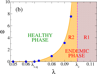
Regions $R_{1}$ and $R_{2}$ make up the endemic phase [see Fig. 3(b)]. According to Eq. (13), when $\lambda$ is above the epidemic threshold of the single network $\lambda_{c}$ the epidemics propagates on the coupled system, independently of the value of the rewiring. This is in agreement with the fact that in region $R_{1}$ the critical rewiring $\omega_{c,q}^{\lambda}$ from Eq. (12) is negative for any value of the parameter’s topology. Since $\omega$ is meaningful only for positive values there is no critical rewiring able to stop the propagation of the epidemics. At the single layer threshold $\lambda_{c}$ the critical rate $\omega_{c,q}^{\lambda}$ diverges, and it is above the region $R_{2}$ that for finite values of $\omega>\omega_{c,q}^{\lambda}$ the two-network system becomes effectively decoupled, and the epidemics cannot propagate. Thus, a high enough rewiring rate can induce an effective rescue of weak endemic states.

In Fig. 3(a) we plot $\omega_{c,q}^{\lambda}$ vs $\lambda$ from Eq. (12) (solid lines). The agreement with the integration of Eqs. (2) (dots) is perfect. Figure 3(b) shows the comparison with simulations of the SIS dynamics on two ER networks with $N=10^{4}$ nodes, average degree $\left<k\right>=10$, and $q=1.0$ for the coupling. To estimate the critical rewiring we performed spreading experiments. They consist on running the dynamics from an initial configuration with a few infected neighboring nodes in layers A and B, and calculating the survival probability $S(t)$ of the run for various values of $\lambda$, i e., the probability that a given run did not reach the healthy state up to time $t$. This probability shows an algebraic decay $S\sim t^{-1}$ at the critical point. We observe that the critical rewiring rate obtained from the simulations (filled circles) coincides with the one predicted by the system of Eqs. (2) (solid line), with a divergence at $1/\left<k\right>=0.1$.

From the eigenvalue Eq. (11), we can also obtain the critical infection rate as a function of $w$

$$\lambda_{c,q}^{w}=\frac{1}{\left(1+q_{w}/2\right)\langle k\rangle},$$ (15)

where

$$q_{w}\equiv\frac{q}{1+w},$$ (16)

which can be interpreted as an effective coupling when the rewiring is present. This is so because Eq. (15) has the same structural form as the expression Eq. (7) for the critical infection rate in a static two-layer network with coupling $q_{w}$. This result indicates that for a fixed interconnectivity $q$, the critical infection rate grows with $\omega$ from $\lambda_{c,q}$ (for $\omega=0$) to $\lambda_{c}$ (for $\omega\to\infty$) [see Fig. (1)]. As we see, the effect of rewiring is then to reduce the coupling between the two layers for the transmission of the disease, even though the “structural coupling” $q$ is not affected by $w$. Therefore, we can think the two-layered system with dynamic interconnections rewired at rate $w$ as a system with static interconnections but with an effective reduced coupling $q_{w}$. An important consequence of Eq. (16) is the fact that $q_{w}\to 0$ in the infinitely fast rewiring limit $w\to\infty$, and thus the endemic phase region $R_{2}$ disappears. This confirms our intuitive idea that when the rewiring is extremely large there are no $IS$ links at the interface and, therefore, layers are effectively decoupled and behave like isolated networks.

V Strong endemic states

We explore in this section how the rewiring affects the epidemics when infection rates are above the single layer threshold $\lambda_{c}$. In this case, the endemic state can be sustained in each network separately, but we shall see that when the layers are interconnected the prevalence depends on the coupling $q$ and the rewiring rate $\omega$. We first make the analysis using the rate equations, which corresponds to the behavior on infinite large systems. Then, we study the case of finite systems, where new phenomenology appears due to the extinction of the epidemics by finite size fluctuations.

V.1 Thermodynamic limit

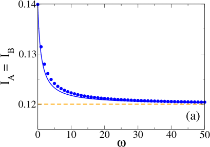
In Fig. 4 we show the prevalence levels $I_{A}$ and $I_{B}$ as a function of the rewiring rate $\omega$, obtained from the numerical integration of equations (2), using $\left<k\right>=10$ and $\left<k_{AB}\right>=0.25$. Fig. 4(a) corresponds to infection rates $\lambda_{A}=\lambda_{B}=\lambda_{AB}=\lambda_{BA}=\lambda=0.115$ above the epidemic threshold $\lambda_{c}=1/\left<k\right>=0.1$, thus each separate network is in the endemic state. As expected, $I_{A}$ and $I_{B}$ reach the same stationary value. We observe that the prevalence decreases monotonically as $\omega$ increases, and approaches the prevalence in the isolated networks (dashed horizontal line) as $\omega$ becomes very large. This behavior is reminiscent of what we found in the last section, that is, both networks become effectively decoupled as $\omega$ goes to infinity, leading to stationary values $I_{A}$ and $I_{B}$ corresponding to single isolated networks. This phenomenon can also be captured from Eqs. (2), by considering the limiting case $\omega\to\infty$. In this limit, the dominant term on the right hand side of Eq. (2d) is $-\omega I_{A}S_{B}$, which gives the exponential time decay $I_{A}S_{B}(t)=(I_{A}S_{B})_{0}\,e^{-\omega t}$, with $(I_{A}S_{B})_{0}$ the initial density of $I_{A}S_{B}$ pairs. That is, the stationary density of $I_{A}S_{B}$ pairs is zero. Following the same argument we obtain from Eq. (2e) that the stationary density of $S_{A}I_{B}$ pairs is also zero. Then, using these two stationary values in Eq. (2f) we get that $I_{A}I_{B}$ is zero as well, due to the combined effects of recovery and rewiring. Finally, from the conservation relation Eq. (1e) we can see that $S_{A}S_{B}=\left<k_{AB}\right>$. In other words, in the infinite rewiring limit the system quickly evolves to a stationary state characterized by the absence of interlinks connecting infected nodes, and thus all interlinks are between susceptible neighbors only. As the disease is only transmitted through infected nodes, there is no possible spreading between networks, which behave effectively as independent on the spreading on its partner network. The complete decoupling leads to a set of three equations corresponding to the evolution of the epidemics on a single network, by setting $I_{A}S_{B}=S_{A}I_{B}=I_{A}I_{B}=0$ in Eqs. (23a), (23) and (23c), whose stationary solution $I_{A}$ is the dashed line in Fig. 4(a).

Figure 4: Prevalence $I_{A}$ and $I_{B}$ in networks A and B, respectively, as a function of the rewiring rate $\omega$. In both graphs we used $\left<k\right>=10$ and $q=0.5$. (a) The infectivities are $\lambda_{A}=\lambda_{B}=\lambda_{AB}=\lambda_{BA}=\lambda=0.115$ above the single layer critical rate $\lambda_{c}=0.1$. The dashed line corresponds to the prevalence in network A or B when isolated. (b) The infectivities are $\lambda_{A}=\lambda_{AB}=0.115$ and $\lambda_{B}=\lambda_{BA}=0.085$, above and below $\lambda_{c}$, respectively. The prevalence in layer B (lower line) is zero when it is isolated, while the prevalence in layer A (upper line) approaches its single layer value $0.12$. Inset: ratio between prevalence in networks A and B as a function of $\omega$.

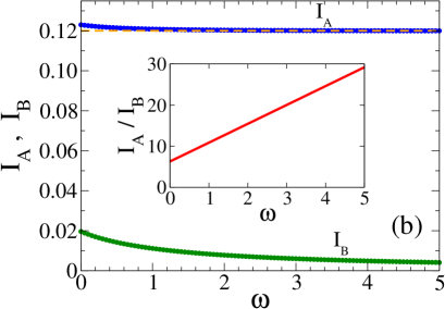As was shown in Saumell-Mendiola et al. (2012), it is not possible to find a mixed phase in the coupled static system, that is, a phase that consists on an endemic state in one layer and a healthy state in the other layer. This is so because when the disease is able to propagate on one layer, then it always propagates on the entire system. This phenomenon is also observed even if the interlinks are rewired, as we see in Fig. 4(b), where we show results from Eq. (2) with infection rates $\lambda_{A}=\lambda_{AB}=0.115>\lambda_{c}=0.1$ and $\lambda_{B}=\lambda_{BA}=0.085<\lambda_{c}=0.1$. Under these asymmetric conditions, the disease is able to spread in layer A but it dies off in layer B, when the networks are disconnected. Again, finite rewiring rates reduce the prevalence in each layer but cannot induce a complete breaking of the coupling, which only happens in the $\omega\to\infty$ limit.

V.2 Finite size effects

In the previous sections we studied the prevalence of the disease in both networks under different scenarios, and how this prevalence is affected by the rewiring of internetwork links, as compared to the case of static interconnections. The analysis was done by means of a system of equations for the densities of nodes and pairs, which is a good mean-field description of the disease dynamics in infinite large networks, where finite size fluctuations are neglected. This allows to study various phenomena that are independent on the system size for large enough networks, such as the transition between the endemic and healthy phase when $\lambda$ and $\omega$ are varied. These equations predict that the disease in the endemic phase last for infinite long times. However, in finite networks, fluctuations in the density of infected nodes in a given realization eventually drive the system to an absorbing configuration, where all nodes are susceptible. This brings new interesting phenomena that are intrinsic of finite systems, and that we explore in this section.

Figure 5: Time evolution of the density of infected nodes $I_{A}$ and $I_{B}$ in networks A and B, respectively, in two distinct realizations of the dynamics (a) and (b), on two coupled ER networks of $N=10^{3}$ nodes each, coupling $q=0.005$ and interlink rewiring $\omega=50$ and $\lambda_{A}=\lambda_{AB}=\lambda_{B}=\lambda_{BA}=\lambda=0.115>\lambda_{c}=0.1$. In realization (a) there is an outbreak in both layers, while in realization (b) the outbreak occurs only in layer A.

We are interested in studying whether the rewiring is able to stop the spreading of the disease from network A to network B, when fluctuations are taken into account. As we showed in section IV.2, the rewiring reduces the effective connectivity between both networks and, as a consequence, it can bring the system from the endemic to the healthy phase when it overcomes a critical rewiring $\omega_{c,q}^{\lambda}$. As explained in section V.1, this is only possible when the infection rates of both networks $\lambda_{A}$ and $\lambda_{B}$ are below the critical infection rate of an isolated network $\lambda_{c}$, otherwise the disease spreads over both networks, independently on the initial condition and the rewiring rate. In other words, when either $\lambda_{A}>\lambda_{c}$ or $\lambda_{B}>\lambda_{c}$, if the disease spreads on A then it spreads on B with probability equal to unity. Only in the $\omega\to\infty$ limit spreading is stopped, because networks are effectively disconnected.

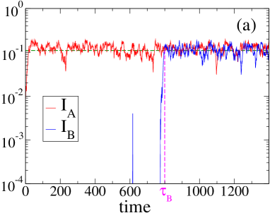
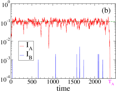
However, we shall see that this scenario is no longer valid in finite networks, where in a single realization of the dynamics with finite $\omega$ (including $\omega=0$), the spreading can take place in one network only. Indeed, Figs. 5(a) and (b) show two distinct realizations with the same parameters and initial condition, but with very different outcomes. Initially, only one random node in network A and its neighbors are infected. We investigate whether this initial small focus of infection propagates through network A, and is able to invade network B. In Fig. 5(a), the disease in network A quickly spreads until it reaches a stationary state in which $I_{A}$ fluctuates around a given value $I^{s}\simeq 0.11$ (horizontal dashed line). We refer to this state where a large fraction of the population gets infected as an outbreak. In network B the outbreak happens at a much longer time $\tau_{B}\simeq 750$, but eventually the disease spreads on both networks, as it happens in infinite systems. However, in fig. 5(b) there is also a quick outbreak in network A but the outbreak in network B never happens, because $I_{A}$ becomes zero by a large fluctuation at time $T_{A}$, driving the entire system to a halt. That is, the epidemics on A goes extinct before the disease can spread on network B. We observe that in various occasions a small fraction of nodes in network B -probably those with connections to network A- get infected, rising $I_{B}$ to values larger than zero that quickly die out, producing a “spike-like” pattern in $I_{B}$. Nevertheless, it seems that $I_{B}$ never reaches a level that is large enough to initiate a cascade of infections that leads to an outbreak.

In the next section we study the statistics of outbreak times $\tau_{B}$ and their associated probabilities. We shall see that the rewiring amplifies finite size effects, inducing a delay in the outbreak of network B that increases with $\omega$, so that the outbreak may remain confined in network A for arbitrary long times. We also show that the there is a finite probability that the disease does not spread on network B.

V.2.1 Outbreak probabilities and times

We ran MC simulations of the dynamics on two coupled ER networks with $N$ nodes each, mean degrees $\langle k\rangle=10$, coupling $q=0.005$ and infection rates $\lambda_{A}=\lambda_{AB}=\lambda_{B}=\lambda_{BA}=\lambda=0.115$. Because $\lambda$ is above the critical value $\lambda_{c}=0.1$, typically an initial seed in network A spreads over a large fraction of the system. When an outbreak happens in A, then the disease can pass to network B through interlinks, and may cause an outbreak in B as well. As we mentioned earlier this is not always the case, because sometimes single infected nodes are not able to initiate an avalanche of massive infections and the disease dies out. We want to estimate the probability $P_{B|A}$ that there is an outbreak in network B given that there was an outbreak in network A. This conditional probability measures the fraction of times that finite size effects amplified by rewiring are not able to stop the “transmission” of an outbreak from A to B. To calculate the outbreak statistics in B conditioned to outbreaks in A, we start the runs from a situation where there is already an outbreak in A, by randomly infecting a fraction $I_{A}=0.12$ of nodes in A, above the prevalence level $I^{s}=0.11$. Starting from a seed in A is not computationally efficient because there is a chance that the disease out in A before an outbreak occurs and, therefore, an outbreak in B neither takes place.

Figure 6: Probability $P_{B|A}$ of an outbreak in layer B after an outbreak happened in layer A of a coupled two-layer system, as a function of the interlink rewiring rate $\omega$. Each layer is an ER network with mean degree $\left<k\right>=10$. The coupling is $q=0.005$ and the infection rates are $\lambda=0.115$. Symbols represent MC simulation results for different system sizes: $N=250$ (squares), $N=500$ (diamonds) and $N=1000$ (circles). Solid lines are the analytic approximations from Eq. (19), while the dashed line is the approximation Eq. (17) using the values $\mu=6.49\times 10^{-5}$ and $\beta=0.0328/(1+\omega)$ calculated in Appendices C and D, respectively.

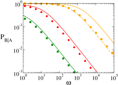In Fig. 6 we plot the outbreak probability in network B, $P_{B|A}$, as a function of the rewiring rate $\omega$, obtained from MC simulations for various system sizes (solid symbols). We observe that $P_{B|A}$ decays very slowly when $\omega$ increases, from a value $P_{B|A}(\omega=0)$ that approaches $1$ as $N$ becomes large ($P_{B|A}(\omega=0)=0.881$ and $0.998$ for $N=500$ and $1000$, respectively). That is, for a static or very slowly varying internetwork connectivity, once the disease spreads on A then it also spreads on B with high probability. But as $\omega$ increases, $I_{A}S_{B}$ links last for shorter times, decreasing the probability of infection of B-nodes and the subsequent outbreak in network B. For $\omega>5\times 10^{4}$ and $N=1000$, the outbreak in B is very unlikely (smaller than $1\%$) , meaning that in most realizations the spreading on B does not happen. Therefore, the rewiring in finite networks proves to be very efficient in preventing the transmisibility between networks. In the next section we show that $P_{B|A}$ decays as $\omega^{-1}$ for $\omega\gg 1$ (solid lines in Fig. 6), thus $P_{B|A}$ becomes zero only in the infinite large rewiring limit $\omega\to\infty$.

Figure 7: Mean outbreak times $\left<\tau_{A}\right>$ (open symbols) and $\left<\tau_{B}\right>$ (filled symbols) in networks A and B, respectively, vs the rewiring rate $\omega$, for a two-layer system with the same parameters and system sizes as in Fig. 6. Solid curves are the analytic approximations from Eq. (20), while the dashed curve is the approximation Eq. (18) with the values $\mu=6.49\times 10^{-5}$ and $\beta=0.0328/(1+\omega)$ calculated in Appendices C and D, respectively. Horizontal dashed lines correspond to numerical results of the mean extinction times in network A.

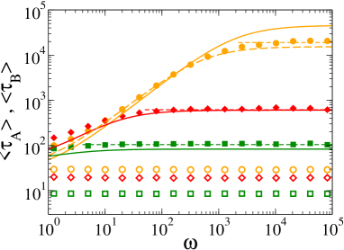In Fig. 7 we show mean outbreak times $\langle\tau_{A}\rangle$ and $\langle\tau_{B}\rangle$ in networks A and B, respectively, over many independent realizations as a function of $\omega$. The mean time $\langle\tau_{A}\rangle$ ($\langle\tau_{B}\rangle$) is an average only over realizations in which network A (network B) undergoes an outbreak. Outbreak times in A were calculated using a seed in A as initial condition. We observe in Fig. 7 that $\langle\tau_{A}\rangle$ is very short and independent on $\omega$, while $\langle\tau_{B}\rangle$ increases monotonically with $\omega$ and reaches a constant value as $\omega\to\infty$. The saturation level $\langle T_{A}\rangle$ corresponds to the mean extinction time in network A when isolated (see Eq. (32) in Appendix C for the scaling of $\langle T_{A}\rangle$ with the model’s parameters). This result is a direct consequence of the fact that the outbreak in B is limited by the extinction in A. Actually, in the very large rewiring limit $\omega\gg 1$ outbreaks in B are very unlikely, but when a B-outbreak does take place it usually happens just before the extinction in network A, so that $\tau_{B}\lesssim T_{A}$ in each realization, and therefore $\langle\tau_{B}\rangle\lesssim\langle T_{A}\rangle$.

In the next section we develop an approach based on a reduced model specially designed to account for the stochastic dynamics of the coupled system of two networks, which allows to obtain analytic expressions for the outbreak probabilities and times.

V.2.2 Three-state symbolic model

In order to gain an insight about the statistics of outbreak times and their probabilities we need to consider the fluctuations associated with the system size. One way to incorporate the stochastic dynamics is to derive a system of equations as the one in section III, but with some additional noise terms corresponding to finite-size fluctuations. This procedure is in general very tedious and hard to carry out because of the large number of processes and equations involved and, besides, only numerical solutions can be obtained. That is why we develop here a much simpler approach, based on a synthetic model specially useful to investigate the outbreak probabilities and times. The approach consists on viewing the system and its dynamics at a coarse-grained level. We represent each network as a simple unit (node), and the state of each network as a binary variable, which is a symbolic representation of the two possible prevalence levels: outbreak when the density of infected nodes $I$ fluctuates around $I^{s}$ (active state), and no-outbreak when $I$ is zero or close to zero (inactive state). This approach is an oversimplification of the complex dynamics of the system, but is able to reproduce rather well the collective properties of extinction and outbreak processes.

Figure 8: Schematic representation of the synthetic model. A red node represents an active network, while a green node denotes an inactive network. $\mu$ and $\beta$ are the effective transition rates between the three possible states of the two-network system.

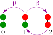In Fig. 8 we show the possible states of the two-node system and their associated transitions. Red and green nodes represent, respectively, active and inactive networks. States 0, 1 and 2 denote the situations in which both networks are inactive, only one network is active, and both networks are active, respectively. These states represent the total activity of the system, so that the two cases A-active/B-inactive and A-inactive/B-active are grouped into a single state 1. An active node becomes inactive at rate $\mu$, and activates its neighboring node at rate $\beta$. The dynamics of this synthetic model is analogous to the one of the SIS model, but with macroscopic transition rates $\mu$ and $\beta$ that are effective rates that depend on the model’s parameters: the network size $N$, the infection rate $\lambda$, the mean connectivity $\langle k\rangle$, the interconnectivity $q$, and the rewiring rate $\omega$. This model tries to capture the time evolution of the outbreak/extinction behavior of the coupled system of two networks. For instance, if at a given time network A is active and network B is inactive (state $1$), we assume that network A triggers an outbreak in network B at constant rate $\beta$ ($1\to 2$ transition), as in Fig. 5(a), and that the disease in network A dies out at constant rate $\mu$ ($1\to 0$ transition), as in Fig. 5(b).

Within this reduced model, the dynamics of transitions between states follows a multiple Poisson process with rates $\mu$ and $\beta$. Therefore, the outbreak probability in network B given an outbreak in A can be estimated as

$$P_{B|A}\simeq P_{12}=\frac{\beta}{\mu+\beta},$$ (17)

and the mean outbreak time in network B as

$$\left<\tau_{B}\right>\simeq\left<\tau_{12}\right>=\frac{1}{\mu+\beta}.$$ (18)

Here $\left<\tau_{12}\right>$ is the mean time of the $1\to 2$ transition normalized by $P_{12}$, that is, over those realizations that made the transition to the outbreak. To check the validity of Eqs. (17) and (18) we run MC simulations to calculate the rates $\mu$ and $\beta$ for networks of size $N=10^{3}$ (see Appendices C and D for details). Dashed lines in Figs. 6 and 7 correspond to Eqs. (17) and (18) using the numerical values of $\mu$ and $\beta$. We observe that the agreement is good, showing that the symbolic model describes quite well the stochastic macroscopic dynamics of the system.

In Appendices C and D we also develop an analytical approach to obtain approximate expressions for $\mu$ [Eq. (33)] and $\beta$ [Eq. (46)]. Plugging Eqs. (33) and (46) into Eqs. (17) and (18) we obtain the following expressions for the outbreak in $B$,

$$P_{B|A} \simeq \left[1+\frac{\mathcal{A}\,e^{-\mathcal{B}N}\,(1+\omega)}{\sqrt{N}\,q}\right]^{-1},$$ (19)

$$\left<\tau_{B}\right> \simeq \left[\mathcal{C}\,\sqrt{N}\,e^{-\mathcal{B}N}+\frac{\mathcal{D}\,q\,N}{1+\omega}\right]^{-1},$$ (20)

where $\mathcal{A=C/D}$, and the coefficients $\mathcal{B,C}$ and $\mathcal{D}$ are given in Eqs. (34), (35) and (D) of the Appendices. Solid curves in Figs. 6 and 7 correspond to Eqs. (19) and (20). Even though we observe a discrepancy with the numerical values (symbols) that increases with the system size, Eqs. (19) and (20) correctly capture the qualitative behavior of $P_{B|A}$ and $\left<\tau_{B}\right>$ with the model’s parameters.

Figure 9: Outbreak probability in network B vs system size $N$ for four different values of the rewiring rate $\omega=1.25$ (circles), $\omega=40$ (squares), $\omega=1280$ (diamonds) and $\omega=40960$ (down triangles). Solid curves are the analytic approximations from Eq. (19).

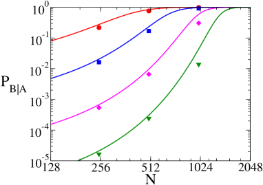
We observe from Eq. (19) and Fig. 6 that for finite and large $N$, $P_{B|A}\lesssim 1$ in a static network $\omega=0$, but it rapidly decreases with the rewiring as $(1+\omega)^{-1}$. Also, $P_{B|A}\to 1$ in the thermodynamic limit, for all finite $\omega$ (see Fig. 9). This is in agreement with the mentioned fact that for infinite large systems in the strong endemic state, an outbreak in A always implies an outbreak in B. In this case, as layer A stays for ever in the endemic state, even if the transmission rate to layer B is reduced to very small values by decreasing $q$ or increasing $\omega$, the disease always ends up invading and breaking up on B. Therefore, we conclude that the rewiring has no effect on the outbreak probability for infinite large networks, but as long as the networks are finite, its effect is amplified as $N$ decreases. From Eq. (20) and Fig. 7 we see that for $\omega\to 0$ mean outbreak times in both networks are similar, while in the opposite limit $\omega\to\infty$, the mean outbreak time in layer B $\left<\tau_{B}\right>$ approaches $1/\mu$, which is similar to the mean extinction time in network A $\left<T_{A}\right>$ (horizontal dashed lines).

VI Summary and Conclusions

We studied a model for disease spreading on two layers of networks coupled through dynamic interconnections. Links connecting infected nodes in different layers are rewired at rate $\omega$ to avoid interlayer contacts between infected and susceptible nodes, so that the interconnecting network coevolves dynamically with the dynamics of the states of the nodes in the two layers. We developed an analytical approach based on the pair approximation to explore the system’s dynamics. This approach reveals that the effect of the rewiring is to reduce the effective coupling between the two layers for the disease transmission, even though the structural coupling is not affected by $\omega$. We find two different mechanisms by which rewiring can stop the propagation of the disease, effectively rescuing endemic states of the global statically interconnected network. Each of these mechanisms is efficient in one of the two scenarios considered of weak or strong endemic states.

In weak endemic states in which the infection rate is below the epidemic threshold of a single layer, the two-layer system with dynamic interconnections can be thought as a system with static interconnections, but with an effective coupling that monotonically decreases with $\omega$. In this case, a high enough rewiring can reduce to zero the disease prevalence found with a static interconnection of layers. This is described in statistical terms by a transition from the endemic to the healthy phase as $\omega$ overcomes a given threshold, which increases with the coupling and the networks’ connectivity.

In strong endemic states in which the infection rate is above the epidemic threshold of a single layer, we studied spreading between layers, starting from a seed of infected nodes in one layer and spreading to the second layer. For a finite size system there is a probability that the infection dies out in the first layer before propagating to the second layer. This probability is practically negligible for a static interconnection, but finite size effects are amplified by interlink rewiring, leading to a finite probability that the epidemics does not propagate to the second layer. The complementary probability that the disease spreads from the infected layer to the susceptible layer in a finite system decreases monotonically with $\omega$, and approaches zero as $\omega\to\infty$.

In summary, our results show that the adaptive rewiring of interlayer links is an effective strategy to control spreading across communities of individuals, either by the existence of a critical rewiring rate that effectively decouples the two communities, or by the amplification of finite size effects that prevent propagation of the disease from one community to the other.

Appendix A Pair approximation approach

The time evolution of the model can be approximately described by the following set of ODEs for nodes and links, which account for state correlations between nearest-neighbors in the networks (first-order correlations):

$$\frac{dI_{A}}{dt} = -I_{A}+\lambda_{A}I_{A}S_{A}+\lambda_{BA}S_{A}I_{B},$$ (21a)

$$\frac{dI_{A}S_{A}}{dt} = 2I_{A}I_{A}-(1+\lambda_{A})I_{A}S_{A}-2\lambda_{A}I_{A}S_{A}I_{A}$$

$$- \lambda_{BA}I_{A}S_{A}I_{B}+\lambda_{A}S_{A}S_{A}I_{A}+\lambda_{BA}S_{A}S_{A}I_{B},$$

$$\frac{dI_{A}I_{A}}{dt} = -2I_{A}I_{A}+\lambda_{A}I_{A}S_{A}+2\lambda_{A}I_{A}S_{A}I_{A}$$ (21c)

$$+ \lambda_{BA}I_{A}S_{A}I_{B},$$

$$\frac{dI_{A}S_{B}}{dt} = I_{A}I_{B}-(1+\omega)I_{A}S_{B}-\lambda_{AB}I_{A}S_{B}$$ (21d)

$$+ \lambda_{A}I_{A}S_{A}S_{B}-\lambda_{B}I_{A}S_{B}I_{B}-2\lambda_{AB}I_{A}S_{B}I_{A}$$

$$+ \lambda_{BA}I_{B}S_{A}S_{B},$$

$$\frac{dS_{A}I_{B}}{dt} = I_{A}I_{B}-(1+\omega)S_{A}I_{B}-\lambda_{BA}S_{A}I_{B}$$ (21e)

$$+ \lambda_{B}S_{A}S_{B}I_{B}-\lambda_{A}I_{A}S_{A}I_{B}-2\lambda_{BA}I_{B}S_{A}I_{B}$$

$$+ \lambda_{AB}S_{A}S_{B}I_{A},$$

$$\frac{dI_{A}I_{B}}{dt} = -2I_{A}I_{B}+\lambda_{AB}I_{A}S_{B}+\lambda_{BA}S_{A}I_{B}$$ (21f)

$$+ \lambda_{A}I_{A}S_{A}I_{B}+\lambda_{B}I_{A}S_{B}I_{B}+2\lambda_{AB}I_{A}S_{B}I_{A}$$

$$+ 2\lambda_{BA}I_{B}S_{A}I_{B}.$$

We have omitted here the rate equations for $I_{B}$, $I_{B}S_{B}$ and $I_{B}I_{B}$ because they have the same form as the equations for $I_{A}$, $I_{A}S_{A}$ and $I_{A}I_{A}$, respectively, after interchanging sub-indices $A$ and $B$. Also, densities $S_{A}$, $S_{B}$, $S_{A}S_{A}$, $S_{B}S_{B}$ and $S_{A}S_{B}$ can be obtained from the conservation relations Eq. (1). We note that the system of equations (21) expresses the evolution of the densities that contain at least one infected node. We shall see that this is particularly convenient when we analyze the stability of the healthy phase.

As we can see, the rate equations for pairs depend on the densities of triplets, for which we use a notation analogous to the ones used for nodes and links. For instance, $I_{A}S_{B}I_{A}$ represents the density per node of triples consisting of an infected node in A connected to a susceptible node in B that is in turn connected to another infected node in A. To close the system of equations  (21) we make use of the pair approximation, which assumes that the links of different types are homogeneously distributed over the networks. This allows to decompose triples in terms of nodes and pairs (see for instance Keeling (1999); Gross et al. (2006); Demirel et al. (2014); Shai and Dobson (2013)), closing the system at the level of pairs. The triplets of Eq. (21) can be expressed as

$$I_{A}S_{A}I_{A} = \frac{I_{A}S_{A}\cdot I_{A}S_{A}}{2S_{A}}\,;~{}~{}I_{A}S_{A}I_{B}=\frac{I_{A}S_{A}\cdot S_{A}I_{B}}{S_{A}},$$

$$I_{A}S_{B}I_{A} = \frac{I_{A}S_{B}\cdot I_{A}S_{B}}{2S_{B}}\,;~{}~{}~{}I_{A}S_{B}I_{B}=\frac{I_{A}S_{B}\cdot I_{B}S_{B}}{S_{B}},$$

$$I_{A}S_{A}S_{A} = \frac{2I_{A}S_{A}\cdot S_{A}S_{A}}{S_{A}}\,;~{}~{}I_{A}S_{A}S_{B}=\frac{I_{A}S_{A}\cdot S_{A}S_{B}}{S_{A}},$$

$$I_{A}S_{B}S_{A} = \frac{I_{A}S_{B}\cdot S_{A}S_{B}}{S_{B}}\,;~{}~{}~{}I_{A}S_{B}S_{B}=\frac{2I_{A}S_{B}\cdot S_{B}S_{B}}{S_{B}}.$$

Replacing the approximate expressions for the triplets from Eq. (A) into the Eqs. (21), we arrive to the system of Eqs. (2) of the main text.

Appendix B Prevalence in a symmetric two-layer system

In this section we derive an analytic expression for the stationary density of infected nodes in a two-layer system with symmetric conditions. For the sake of simplicity, we first analyze the case of a single islolated, and then adapt the results for the case of two coupled networks.

Applying the pair approximation developed in Appendix A for the case of a single network, for instance network A, we can describe the evolution of the system by the set of equations

$$\frac{dI_{A}}{dt} = -I_{A}+\lambda I_{A}S_{A},$$ (23a)

$$\frac{dI_{A}S_{A}}{dt} = 2I_{A}I_{A}-(1+\lambda)I_{A}S_{A}-\lambda\frac{(I_{A}S_{A})^{2}}{S_{A}}~{}~{}~{}~{}~{}~{}$$

$$+ 2\lambda\frac{S_{A}S_{A}\cdot I_{A}S_{A}}{S_{A}},$$

$$\frac{dI_{A}I_{A}}{dt} = -2I_{A}I_{A}+\lambda I_{A}S_{A}+\lambda\frac{(I_{A}S_{A})^{2}}{S_{A}},$$ (23c)

together with the conservation relations

$$1 = I_{A}+S_{A},$$ (24a)

$$\frac{\left<k\right>}{2} = S_{A}S_{A}+I_{A}I_{A}+I_{A}S_{A},$$ (24b)

where $I_{A}$, $I_{A}S_{A}$ and $I_{A}I_{A}$ are, respectively, the densities of $I_{A}$ nodes, $I_{A}S_{A}$ links and $I_{A}I_{A}$ links. Notice that these equations can be derived from Eqs. (2) by setting $\lambda_{BA}=0$ (A isolated from B). To find the stationary density of infected nodes $I_{A}^{s}$ from Eqs. (23), we set the derivatives to zero and express the stationary densities of links $[S_{A}S_{A}]^{s}$ and $[I_{A}S_{A}]^{s}$ and $[I_{A}I_{A}]^{s}$ in terms of $I_{A}^{s}$, using the relation Eq. (24a). We obtain

$$\left[S_{A}S_{A}\right]^{s} = \frac{1-I_{A}^{s}}{2\lambda}$$

$$\left[I_{A}S_{A}\right]^{s} = \frac{I_{A}^{s}}{\lambda}$$

$$\left[I_{A}I_{A}\right]^{s} = \frac{I_{A}^{s}}{2}\left[1+\frac{I_{A}^{s}}{\lambda(1-I_{A}^{s})}\right].$$

Finally, plugging these expressions into Eq. (24b) we arrive to the following quadratic equation for $I_{A}^{s}$

$$\lambda(I_{A}^{s})^{2}-\lambda(1+\left<k\right>)I_{A}^{s}+\lambda\left<k\right>-1=0.$$ (25)

Only the solution of Eq. (25) corresponding to the negative branch has a physical meaning, which reads

$$I_{A}^{s}=\frac{1+\lambda_{c}}{2\lambda_{c}}-\sqrt{\left(\frac{1-\lambda_{c}}{2\lambda_{c}}\right)^{2}+\frac{1}{\lambda}},$$ (26)

where $\lambda_{c}=\left<k\right>^{-1}$ is the critical infection rate of the network.

In the symmetric and homogeneous case scenario of two identical coupled networks A and B, with mean degree $\left<k\right>$, infection rates $\lambda_{A}=\lambda_{AB}=\lambda_{BA}=\lambda_{B}=\lambda$ and coupling $q$, the static two-network system can be treated as a single network with mean degree $\left<k\right>+\left<k_{AB}\right>=(1+q/2)\left<k\right>$ and infection rate $\lambda$. Therefore, using Eq. (26), the stationary density of infected nodes in the symmetric two-layer system is

$$I^{s}_{A,q}=\frac{1+\lambda_{c,q}}{2\lambda_{c,q}}-\sqrt{\left(\frac{1-\lambda_{c,q}}{2\lambda_{c,q}}\right)^{2}+\frac{1}{\lambda}},$$ (27)

where $\lambda_{c,q}=[(1+\frac{q}{2})\left<k\right>]^{-1}$ is the critical infection rate of the static coupled system. For a dynamic system with interlink rewiring $\omega$, we showed in section IV.2 that the coupling becomes $q_{\omega}=q/(1+\omega)$, and thus we expect the stationary density of infected nodes to behave as

$$I^{s}_{A,q,\omega}=\frac{1+\lambda_{c,q}^{\omega}}{2\lambda_{c,q}^{\omega}}-\sqrt{\left(\frac{1-\lambda_{c,q}^{\omega}}{2\lambda_{c,q}^{\omega}}\right)^{2}+\frac{1}{\lambda}},$$ (28)

with $\lambda_{c,q}^{\omega}=[(1+\frac{q_{\omega}}{2})\left<k\right>]^{-1}$ the infection threshold. Equation (28) agrees reasonably well with the numerical integration of the system of Eqs. (2) for the two-network system [see Figs. 2 and 4(a)]. The agreement is very good for $\omega$ close to $\omega_{c,q}^{\lambda}$, because the ansatz relation Eq. (16) that we used for the effective coupling is only exact at the transition point (as we derived in section IV.2), that is, when $I_{A}=I_{B}=0$. The agreement is also perfect for $\omega=0$, because the solution Eq. (27) is exact, while discrepancies arise between between $\omega=0$ and $\omega_{c,q}^{\lambda}$

Appendix C Calculation of the extinction rate $\mu$

To calculate the effective rate $\mu$ at which the epidemics extinguishes on a single isolated network, we run MC simulations on an ER network of $N=10^{3}$ nodes, mean degree $\left<k\right>=10$ and infection rate $\lambda=0.115$, starting from an initial density $I(0)=0.11$ of infected nodes that corresponds to the stationary active state. Then, we calculate the survival probability $S(t)$, that is, the probability that the epidemics is not extincted up to time $t$. Working with survival probabilities rather than first-passage probabilities is better because fluctuations are smaller. Within the synthetic model, where we assume a constant decay rate from the active to the inactive state, we expect an exponential decay of the form $e^{-\mu t}$ for the survival probability. In simulations, this decay is observed after a very short initial transient $\hat{t}\simeq 50$, during which $S$ is nearly constant. Thus, we can approximate the shape of $S$ as

$$S(t)\simeq\left\{\begin{array}[]{ll}1&\mbox{for}~{}~{}t\leq\hat{t}\\ e^{-\mu(t-\hat{t})}&\mbox{for}~{}~{}t>\hat{t}.\end{array}\right.$$ (31)

The slope of the $S$ vs $t$ curve on a linear-log plot gives $\mu\simeq 6.49\times 10^{-5}$ (dashed curve in Fig. 10).

An analytical expression for the upper bound of the average life time $\left<T\right>$ of the SIS model on an arbitrary network was given by Van Mieghem in Van Mieghem (2013). It reads,

$$\left<T\right>\simeq\frac{\frac{\lambda}{\lambda_{c}}\,\sqrt{2\pi}\,\exp\Big{\{}\left[\ln\left(\frac{\lambda}{\lambda_{c}}\right)+\frac{\lambda_{c}}{\lambda}-1\right]N\Big{\}}}{\left(\frac{\lambda}{\lambda_{c}}-1\right)^{2}\sqrt{N}},$$ (32)

where $N$ is the network size and $\lambda_{c}$ is the epidemic threshold. Plugging the expression $\lambda_{c}=1/\left<k\right>$ for an ER network on Eq. (32), and given that $\mu\simeq 1/\left<T\right>$, we arrive to the following expression for a lower bound of the extinction rate

$$\mu \simeq \mathcal{C}\,\sqrt{N}\,e^{-\mathcal{B}N},$$ (33)

with

$$\mathcal{B} \equiv \ln\left(\lambda\left<k\right>\right)+\frac{1}{\lambda\left<k\right>}-1~{}~{}~{}~{}\mbox{and}$$ (34)

$$\mathcal{C} \equiv \frac{\left(\lambda\left<k\right>-1\right)^{2}}{\lambda\left<k\right>\sqrt{2\pi}}.$$ (35)

For $N=10^{3}$, $\left<k\right>=10$ and $\lambda=0.115$ we get $\mu\simeq 2.2\times 10^{-5}$, which is approximately $1/3$ of the numerical value $\mu\simeq 6.49\times 10^{-5}$ obtained from simulations. The reason for this discrepancy is because we expect the numerical value of $\mu$ to be larger than the lower bound given by Eq. (33). Even though Eq. (33) is not precise, it captures the right qualitative behavior of $\mu$ with $\lambda$, $\left<k\right>$ and $N$. Indeed, we notice that the coupling between the layers has no effect on $\mu$, as it is independent of $q$ and $\omega$. This is because we assume that the extinction in layer A is not affected by layer B, as long as B is in the inactive state (see Fig. 8). We also observe that $\mu\to 0$ as $N\to\infty$, in agreement with the fact that for $\lambda>\lambda_{c}$ an infinite large system never decays to the healthy state. That is, once there is an outbreak in layer A, the transition back to the healthy state is only possible in finite systems.

Appendix D Calculation of the outbreak rate $\beta$

To obtain the outbreak rate $\beta$ we run MC simulations on two interconnected ER networks A and B, of $N=10^{3}$ nodes each, mean degree $\left<k\right>=10$, $\lambda=0.115$ and coupling $q=0.005$, starting from a density $I_{A}(0)=0.11$ and $I_{B}(0)=0$ of infected nodes in A and B, respectively. We stop the simulation when either $I_{A}$ becomes zero ($1\to 0$ transition) or $I_{B}$ overcomes the value $I^{s}=0.11$ by the first time ($1\to 2$ transition). This corresponds to having the system initially in state $1$, with A active and B inactive (see Fig. 8), and calculating the first-passage statistics to either state $0$ or $2$. Given that $\beta$ is a measure of the likelihood that the disease is transmitted from A to B, we expect $\beta$ to decrease as the rewiring rate $\omega$ increases. Therefore, we run simulations for several values of $\omega$ to study this dependence. To obtain the transition rates, it proves useful to work with the persistence probability in state $1$, $S_{1}(t)$, i e., the probability that the system did not leave state $1$ up to time $t$. Given that the total outgoing rate from state $1$ is $\mu+\beta$, we expect the persistence probability to behave as

$$S_{1}(t)\simeq e^{-(\mu+\beta)t}.$$ (36)

Figure 10: Persistence probability in state $1$ $S_{1}$ vs time, for two coupled networks of $N=10^{3}$ nodes each, mean degree $\left<k\right>=10$, coupling $q=0.005$ and infection rate $\lambda=1$. Each solid curve corresponds to a different value of the rewiring rate $\omega=1280,640,320,160,80,40,20,10$ and $0$ (from top to bottom). The dashed curve at the top corresponds to the survival probability $S$ of a single network. We note that the slope $\alpha$ of $S_{1}$ approaches the slope $\mu$ of $S$ as $\omega$ increases.

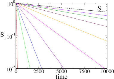
As it happens for the single-network survival probability $S(t)$, we found from MC simulations that $S_{1}(t)$ is nearly constant up to a time $\hat{t}\simeq 50$, and then decays exponentially fast to zero (see Fig. 10):

$$S_{1}(t)\simeq\left\{\begin{array}[]{ll}1&\mbox{for}~{}~{}t\leq\hat{t}\\ e^{-\alpha(t-\hat{t})}&\mbox{for}~{}~{}t>\hat{t},\end{array}\right.$$ (39)

where the exponent $\alpha$ depends on the rewiring rate $\omega$. Again, it seems that after a time $\hat{t}$ the dynamics of the two-network system behaves, at a coarse-grained level, as the one of a three-state system with effective transition rates. We observe in Fig. 10 that $S_{1}$ approaches $S$ as $\omega$ increases. This is consistent with the fact that at very large rewiring rates network A decouples from network B. Thus, A behaves as a single network, independent from B and, therefore, the only possible process is the extinction from the initial active state in A.

Comparing Eqs. (36) and (39) we obtain the relation

$$\alpha=\mu+\beta.$$ (40)

Figure 11: Outbreak transition rate $\beta$ vs rewiring rate $\omega$. Solid circles were calculated from the slopes $\alpha$ of the persistent probability $S_{1}$ of Fig. 10, using the formula $\beta=\alpha-\mu$, with the extinction rate $\mu=6.49\times 10^{-5}$. The solid line corresponds to the fitting function $c/(1+\omega)$, where $c=0.0328$ is the best fitting parameter.

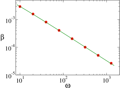
In Fig. 11 we plot $\beta=\alpha-\mu$ vs $\omega$, using the measured values of $\alpha$ from Fig. 10 and the value $\mu=6.49\times 10^{-5}$ calculated in Appendix C. The data is well fitted by the function $\beta(w)=c/(1+\omega)$, with $c=0.0328$. This means that $\beta$ vanishes as $\omega$ goes to infinity, showing that the outbreak transition $1\to 2$ is strictly zero only in the $\omega\to\infty$ limit.

We now obtain an analytical expression for $\beta$. Starting from an initial condition consisting of an outbreak in network A and no infected nodes in network B (state 1), we assume that a node in B gets infected (“infection seed”) at a rate $\Lambda$, and that this seed grows generating an outbreak with probability $S_{\infty}$. Therefore, $\beta$ is estimated as

$$\beta=\Lambda\,S_{\infty}.$$ (41)

That is, every mean time interval $1/\Lambda$ a seed is planted in B, which grows and becomes an outbreak with probability $S_{\infty}$, and thus the outbreak probability per time is as in Eq. (41). Here

$$S_{\infty}\equiv\lim_{t\to\infty}S(t),$$

where $S(t)$ is the survival probability in a spreading experiment, i e., the probabilility that a run starting from a seed survives up to time $t$. Based on a rigorous proof for spreading models with absorbing states Durrett (1988), we expect the ultimate survival probability to be equivalent to the density of nodes in the stationary state,

$$S_{\infty}=I^{s}.$$ (42)

Besides, the total infection rate from A to B, $\Lambda$, should be proportional to the total number of interlinks of type $I_{A}S_{B}$ and the infection rate per link $\lambda$, that is

$$\Lambda=\lambda NI_{A}S_{B}.$$ (43)

Here $I_{A}S_{B}$ is the stationary density of links connecting an infected node in A and a susceptible node in B, which is estimated as $I_{A}S_{B}=I_{A}^{s}\left<k_{AB}\right>=I_{A}^{s}\,q\left<k\right>/2(1+\omega)$, given that all nodes in B are susceptible. We have also used the effective coupling $q_{\omega}=q/(1+\omega)$ for a dynamic network, which accounts for the reduction of the number of interlayer links between infected and susceptible nodes when the rewiring is switched on. Plugging this expression for $I_{A}S_{B}$ into Eq. (43) we obtain

$$\Lambda=\frac{\lambda\,q\left<k\right>NI_{A}^{s}}{2(1+\omega)}.$$ (44)

Finally, replacing the expressions for $S_{\infty}$ and $\Lambda$ from Eqs. (42) and (44) into Eq. (41) leads to

$$\beta=\frac{\lambda\,q\left<k\right>N(I_{A}^{s})^{2}}{2(1+\omega)}.$$ (45)

Using the values of the model’s simulations $N=10^{3}$, $\left<k\right>=10$, $\lambda=0.115$ and $I_{A}^{s}=0.11$ in Eq. (45) we get $\beta=c/(1+\omega)$, with $c\simeq 0.0348$, which is comparable to the best fitting parameter $0.0328$ of Fig. 11 (about $6\%$ difference). This shows that Eq. (45) is a good approximation for $\beta$, for the parameters used in the simulation.

To complete the analytic expression for $\beta$ in terms of the model’s parameters, we insert into Eq. (45) the analytical expression Eq. (26) for $I_{A}^{s}$ obtained in section B, and replace back $\lambda_{c}$ by $\left<k\right>^{-1}$. We finally arrive to

$$\beta\simeq\frac{\mathcal{D}\,q\,N}{1+\omega},$$ (46)

with

$$\mathcal{D}\equiv\frac{\lambda\,\left<k\right>}{2}\left(\frac{1+\left<k\right>^{2}}{2}+\frac{1}{\lambda}-\frac{1+\left<k\right>}{2}\sqrt{\left(1-\left<k\right>\right)^{2}+\frac{4}{\lambda}}\right).$$

From Eq. (46) we see that $\beta$ increases linearly with $q$ and $N$. This happens because $\beta$ is proportional to the total number of infections from nodes in A to nodes in B through interlayer links, which are proportional to $q$ and $N$. In particular, A has no effect on B ($\beta=0$) when $q=0$. We also observe that $\beta$ decreases monotonically with $\omega$, showing that the rewiring reduces the transmission rate of the disease from A to B.

References

- DeDomenico et al. (2013) M. DeDomenico, A. Sole-Ribalta, E. Cozzo, M. Kivela, Y. Moreno, M. A. Porter, S. Gomez, and A. Arenas, Physical Review X 3, 041022 (2013).
- Kivela et al. (2014) M. Kivela, A. Arenas, M. Barthelemy, J. Gleeson, Y. Moreno, and M. A. Porter, Journal of Complex Networks 2, 203 (2014).
- Domenico et al. (2015) M. D. Domenico, V. Nicosia, A. Arenas, and V. Latora, Nature Communications 6 (2015).
- Diakonova et al. (2015a) M. Diakonova, V. Nicosia, V. Latora, and M. San Miguel, arXiv:1507.08940 (2015a).
- Saumell-Mendiola et al. (2012) A. Saumell-Mendiola, M. A. Serrano, and M. Boguñá, Phys Rev E 86, 026106 (2012).
- Dickison et al. (2012) M. Dickison, S. Havlin, and H. E. Stanley, Phys Rev E 85, 066109 (2012).
- Buono C. and L. (2014) M. P. Buono C., Alvarez-Zuzek L. and B. L., PLoS ONE 9, e92200 (2014).
- Granell et al. (2014) C. Granell, S. Gómez, and A. Arenas, Phys Rev E 90, 012808 (2014).
- Sanz et al. (2014) J. Sanz, C.-Y. Xia, S. Meloni, and Y. Moreno, Physical Review X 4, 041005 (2014).
- Barrat et al. (2004) A. Barrat, M. Barthelemy, R. Pastor-Satorras, and A. Vespignani, Proc. Natl. Acad. Sci. USA 101 (11), 3747 (2004), eprint cond-mat/0311416v1.
- Holme and Saramaki (2013) P. Holme and J. Saramaki, Temporal Networks (Springer, 2013).
- Zimmermann et al. (2001) M. G. Zimmermann, V. M. Eguiluz, and M. San Miguel, Economics with Heterogeneous Interacting Agents, vol. 503 (Springer Berlin, 2001).
- Zimmermann et al. (2004) M. G. Zimmermann, V. M. Eguiluz, and M. San Miguel, Physical Review E 69, 065102 (2004).
- Gross and Blasius (2008) T. Gross and B. Blasius, Journal of the Royal Society Interface 5, 259 (2008).
- Gross and Sayama (2009) T. Gross and H. Sayama, Adptive Networks: Theory, Models and Applications (Springer Verlag, New York, 2009).
- Vazquez (2013) F. Vazquez, Opinion dynamics on coevolving networks, vol. 2 (Springer New York, 2013).
- Gross et al. (2006) T. Gross, C. J. D. D’Lima, and B. Blasius, Phys Rev Lett 96, 208701 (2006).
- Vazquez et al. (2008) F. Vazquez, V. M. Eguiluz, and M. S. Miguel, Phys. Rev. Lett. 100, 108702 (2008).
- Diakonova et al. (2015b) M. Diakonova, V. M. Eguíluz, and M. San Miguel, Physical Review E 92, 032803 (2015b).
- Vazquez et al. (2007) F. Vazquez, J. C. González-Avella, V. M. Eguíluz, and M. San Miguel, Physical Review E 76, 046120 (2007).
- Shai and Dobson (2013) S. Shai and S. Dobson, Phys Rev E 87, 042812 (2013).
- Diakonova et al. (2014) M. Diakonova, V. M. Eguiluz, and M. San Miguel, Physical Review E 89, 0652818 (2014).
- Gillespie (2001) D. Gillespie, Journal of Chemical Physics 115, 1716 (2001).
- Demirel et al. (2014) G. Demirel, F. Vazquez, G. Böhme, and T. Gross, Physica D 267, 68 (2014).
- Pastor-Satorras and Vespignani (2001) R. Pastor-Satorras and A. Vespignani, Phys. Rev. Lett. 86, 3200 (2001).
- Luo et al. (2014) X.-F. Luo, X. Zhang, G.-Q. Sun, and Z. Jin, Physica A 410, 144 (2014).
- Keeling (1999) M. J. Keeling, Proc. Roy. Soc. Lond. B 266, 859 (1999).
- Van Mieghem (2013) P. Van Mieghem, arXiv:1310.3980 (2013).
- Durrett (1988) R. Durrett, Lecture Notes on Particle Systems and Percolation (Wadsworth & Brooks/Cole, Pacific Grove, CA, 1988).