Geometric analysis of pathways dynamics: application to versatility of TGF-$\beta$ receptors

Abstract

We propose a new geometric approach to describe the qualitative dynamics of chemical reactions networks. By this method we identify metastable regimes, defined as low dimensional regions of the phase space close to which the dynamics is much slower compared to the rest of the phase space. Given the network topology and the orders of magnitude of kinetic parameters, the number of such metastable regimes is finite. The dynamics of the network can be described as a sequence of jumps from one metastable regime to another. We show that a geometrically computed connectivity graph restricts the set of possible jumps. We also provide finite state machine (Markov chain) models for such dynamic changes. Applied to signal transduction models, our approach unravels dynamical and functional capacities of signaling pathways, as well as parameters responsible for specificity of the pathway response. In particular, for a model of TGF$\beta$ signalling, we find that the ratio of TGFBR1 to TGFBR2 concentrations can be used to discriminate between metastable regimes. Using expression data from the NCI60 panel of human tumor cell lines, we show that aggressive and non-aggressive tumour cell lines function in different metastable regimes and can be distinguished by measuring the relative concentrations of receptors of the two types.

Keywords: tropical Geometry, cancer systems biology, finite state automaton, metastability.

1 Introduction

Networks of biochemical reactions are used in computational biology as models of signaling, metabolism, and gene regulation. For various applications it is important to understand how the dynamics of these models depend on internal parameters, initial data and environment variables. Traditionally, the dynamics of biochemical networks is studied in the framework of chemical kinetics that can be either deterministic (ordinary differential equations) or stochastic (continuous time Markov processes). In order to cope with qualitative data, boolean or multi-valued networks are used instead of continuous models. Large network models have as major inconvenience the difficulty to analyse and classify their possible dynamic behaviors. For instance, the number of states of multi-valued networks with $m$ levels (boolean networks correspond to $m=2$) is $m^{n}$, which generates exponential complexity of the phase space exploration.

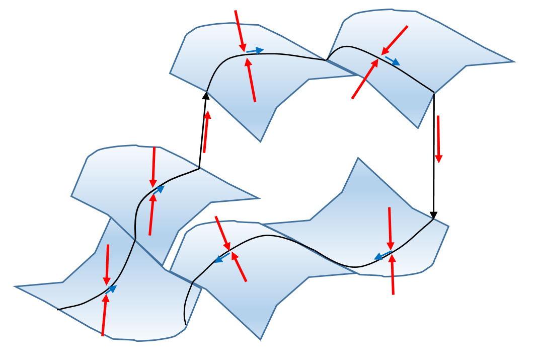
In this paper we propose a new method for model analysis that uses coarse grained descriptions of continuous dynamics as discrete automata defined on finite states. These states will not be obtained by discretization of network variables, but by discretization of collective modes describing possible coordinated activity of several variables. For large networks with ordinary differential equations dynamics and multiple timescales it is reasonable to consider the following property: a typical trajectory consists in a succession of qualitatively different slow segments separated by faster transitions. The slow segments, generally called metastable states or regimes, can be of several types such as attractive invariant manifolds [9], Milnor attractors [25] or saddle connections [24]. The notion of metastability generalizes the notion of attractor. Like in the case of attractors, distant parts of the system can have have coordinated activity for metastability. This coordination can be abstractly represented by the proximity to a lower dimension hypersurface in the phase space. A system remains in the proximity of an attractor after entering its basin of attraction, but can leave a metastable regime after a more or less long time. As illustrated in Fig.1 several such transitions can happen successively. This phenomenon, called itinerancy received particular attention in neuroscience [37]. We believe that similar phenomena occur in molecular biology for chemical reaction networks. A simple example sustaining this picture is the set of bifurcations of metastable states guiding the orderly progression of the cell cycle [20]. In such models, biological distinct stages such as interphase and mitosis correspond to relatively slow segments of the dynamics and are separated by fast transitions. During these stages, several biochemical variables have coordinated activity.

We will use tropical geometry methods to compute metastable dynamic regimes of chemical reaction networks with polynomial or rational kinetic laws. Tropical methods [14, 16], also known as idempotent or max-plus algebras due their name to the fact that one of the pioneer of the field, Imre Simon, was Brazilian. These methods found numerous applications to computer science [34], physics [14], railway traffic [2], and statistics [22]. Recently we have applied these methods to model order reduction [20, 21, 26, 30]. In these works we have used tropical methods to rank monomial terms into rate vectors according to their orders of magnitude and to identify lowest order, dominant terms. When there is only one dominant term or when the dominant terms have all the same sign, the dynamics is fast and the system tends rapidly towards a region in phase space where at least two dominant terms of opposite signs are equilibrated. We have called the latter situation tropical equilibration. In this paper, we use tropical equilibrations to identify metastable dynamic regimes of chemical reaction networks. We show that tropical equilibrations can be grouped into branches and describe the qualitative network dynamics as a sequence of transitions from one branch to another. The complexity of the qualitative dynamics depends on the number of branches. Therefore, we would like to know how this number depends on the number of chemical species. Although there are theoretical results suggesting that the number of branches should be small, these results are valid in the average in the probabilistic space of all the models. In order to test this property numerically we will compute the branches for a large collection of models of the Biomodels database.

The structure of the paper is as follows. In the second section we introduce the branches of tropical equilibrations and discuss briefly how they can be calculated. In the third section we apply the computation of branches to models in the Biomodels database. In the forth section we propose an algorithm to learn Markov state models defined on branches of tropical equilibrations. In the fifth section we apply the method to a model of TGF$\beta$ signaling and show how the analysis can be used to interpret biological data.

Figure 1: Abstract representation of metastability as itinerant trajectory in a patchy phase space landscape. Dominant vector fields (red arrows) confine the trajectory to low dimensional patches on which act weak uncompensated vector fields (blue arrows). A typical trajectory contains slow segments within patches where dominant vector fields cancel, and transitions between patches in the fast direction of uncancelled dominant vector fields. Continuous (but non smooth) connections are also possible, corresponding to role reversal between dominant and dominated vector fields. The term crazy-quilt was coined to describe such a patchy landscape [6].

2 Tropical equilibrations of chemical reactions networks with polynomial rate functions

In this section we introduce the main concepts relating geometry and dynamics.

We consider chemical reaction networks described by mass action kinetics

$$\frac{\mathrm{d}x_{i}}{\mathrm{d}t}=\sum_{j}k_{j}S_{ij}x^{\alpha_{j}},\,1\leq i\leq n,$$ (1)

where $k_{j}>0$ are kinetic constants, $x_{i}$ are variable concentrations, $S_{ij}\in{\mathbb{Z}}$ are the integer entries of the stoichiometric matrix, $\alpha_{j}=(\alpha_{1}^{j},\ldots,\alpha_{n}^{j})$ are multi-indices, and $x^{\alpha_{j}}=x_{1}^{\alpha_{1}^{j}}\ldots x_{n}^{\alpha_{n}^{j}}$, where $\alpha_{i}^{j}$ are positive integers.

For our reasonings, we can replace the exact values of parameters by their orders of magnitude. Usually, orders of magnitude are approximations of the parameters by integer powers of ten and serve for rough comparisons. Our definition of orders of magnitude is based on the equation $k_{j}=\bar{k}_{j}\varepsilon^{\gamma_{j}}$, where $\epsilon$ is a small positive number. The exponents $\gamma_{j}$ are considered to be integer or rational. For instance, the approximation

$$\gamma_{j}=\text{round}(\log(k_{j})/\log(\varepsilon)),$$ (2)

produces integer exponents, whereas $\gamma_{j}=\text{round}(d\log(k_{j})/\log(\varepsilon))/d$ produces rational exponents, where round stands for the closest integer (with half-integers rounded to even numbers) and $d$ is a strictly positive integer. When $\epsilon=1/10$, our definition provides the usual decimal orders.

Kinetic parameters are fixed. In contrast, species orders vary in time and have to be computed. To this aim, the species concentrations are first represented by orders of magnitude defined as

$$a_{j}=\log(x_{j})/\log(\varepsilon).$$ (3)

Because $\log(\varepsilon)<0$, Eq.(3) means that species orders and concentrations are anti-correlated (large orders mean small concentrations and vice versa).

Then, network dynamics is described by a rescaled ODE system

$$\frac{\mathrm{d}\bar{x}_{i}}{\mathrm{d}t}=\sum_{j}\varepsilon^{\mu_{j}(a)-a_{i}}\bar{k}_{j}S_{ij}{\bar{x}}^{\alpha_{j}},$$ (4)

where

$$\mu_{j}(a)=\gamma_{j}+\langle a,\alpha_{j}\rangle,$$ (5)

and $\langle,\rangle$ stands for the dot product.

The r.h.s. of each equation in (4) is a sum of multivariate monomials in the concentrations. The orders $\mu_{j}$ indicate how large are these monomials, in absolute value. A monomial of order $\mu_{j}$ dominates another monomial of order $\mu_{j^{\prime}}$ if $\mu_{j}<\mu_{j^{\prime}}$.

To set these ideas down let us use a simple chemical network example, the Michaelis-Menten kinetics:

$$S+E\underset{k_{-1}}{\overset{k_{1}}{\rightleftharpoons}}ES\overset{k_{2}}{\rightarrow}P+E,$$

where $S,ES,E,P$ represent the substrate, the enzyme-substrate complex, the enzyme and the product, respectively.

After using the two conservation laws $E+ES=e_{0}$ and $S+ES+P=s_{0}$, we find

$$\begin{split}\dot{x}_{1}&=-k_{1}x_{1}(e_{0}-x_{2})+k_{-1}x_{2},\\ \dot{x}_{2}&=k_{1}x_{1}(e_{0}-x_{2})-(k_{-1}+k_{2})x_{2}.\end{split}$$ (6)

where $x_{1}$, $x_{2}$ are the concentrations of $S$ and $ES$ respectively.

Orders of variables and parameters are as follows $x_{i}=\bar{x}_{i}\epsilon^{a_{i}}$, $1\leq i\leq 2$, $k_{1}=\bar{k}_{1}\epsilon^{\gamma_{1}}$, $k_{-1}=\bar{k}_{-1}\epsilon^{\gamma_{-1}}$, $e_{0}=\bar{e}_{0}\epsilon^{\gamma_{e}}$.

The tropical equilibration problem consists in the equality of the orders of at least two monomials one positive and another negative in the differential equations of each species. This condition allows us to compute the concentration orders defined by (3). More precisely, we want to find a vector $a$ such that

$$\min_{j,S_{ij}>0}(\gamma_{j}+\langle a,\alpha_{j}\rangle)=\min_{j,S_{ij}<0}(\gamma_{j}+\langle a,\alpha_{j}\rangle)$$ (7)

The equation(7) is related to the notion of tropical hypersurface. A tropical hypersurface is the set of vectors $a\in{\mathbb{R}}^{n}$ such that the minimun $\min_{j,S_{ij}\neq 0}(\gamma_{j}+\langle a,\alpha_{j}\rangle)$ is attained for at least two different indices $j$ (with no sign conditions). Tropical prevarieties are finite intersections of tropical hypersurfaces. Therefore, our tropical equilibrations are subsets of tropical prevarieties [16]. The sign condition in (7) was imposed because species concentrations are real positive numbers. Compensation of a sum of positive monomials is not possible for real values of the variables.

The system (7) can be seen as a system of equations in min-plus algebra (also known as tropical semiring), where multiplication $\otimes$ is the real numbers addition $x\otimes y=x+y$ and the addition $\oplus$ is the minimum operation $x\oplus y=\min(x,y)$. In order to find the solutions of such system we can explore combinatorially trees of solutions resulting from various choices of minimal terms and write down inequations for each situation. Because a set of inequations define a polyhedron, the set of tropical equilibration solutions forms a polyhedron in ${\mathbb{R}}^{n}$. As a matter of fact, computing tropical equilibrations from the orders of magnitude of the model parameters is a NP-complete problem [36] and brute force calculation by exploration of combinatorics has exponential complexity. However, methods based on the Newton polytope [31] or constraint logic programming [35] exploit the sparseness and redundancy of the system and reduce the combinatorics and the time to compute tropical solutions.

The tropical equilibration equations for the Michaelis-Menten example are obtained by equating minimal orders of positive monomials with minimal orders of negative monomials in (6):

$$\gamma_{1}+\gamma_{e}+a_{1} =\min(\gamma_{1}+a_{1},\gamma_{-1})+a_{2},$$ (8)

$$\gamma_{1}+\gamma_{e}+a_{1} =\min(\gamma_{1}+a_{1},\min(\gamma_{-1},\gamma_{2}))+a_{2}.$$ (9)

Species timescales. The timescale of a variable $x_{i}$ is given by $\frac{1}{x_{i}}\frac{\mathrm{d}x_{i}}{\mathrm{d}t}=\frac{1}{\bar{x}_{i}}\frac{\mathrm{d}\bar{x}_{i}}{\mathrm{d}t}$ whose order is

$${\nu_{i}=\min\{\mu_{j}|S_{ij}\neq 0\}-a_{i}}.$$ (10)

The order $\nu_{i}$ indicates how fast is the variable $x_{i}$ (if $\nu_{i^{\prime}}<\nu_{i}$ then $x_{i^{\prime}}$ is faster than $x_{i}$) .

Partial tropical equilibrations. It is useful to extend the tropical equilibration problem to partial equilibrations, that means solving (7) only for a subset of species. This is justified by the fact that slow species do not need to be equilibrated. In order to have a self-consistent calculation we compute the species timescales by (10). A partial equilibration is consistent if $\nu_{i}<\nu$ for all non-equilibrated species $i$. $\nu>0$ is an arbitrarily chosen threshold indicating the timescale of interest.

Tropical equilibrations, slow invariant manifolds and metastable dynamic regimes. In dissipative systems, fast variables relax rapidly to some low dimensional attractive manifold called invariant manifold [9] that carries the slow mode dynamics. A projection of dynamic equations onto this manifold provides the reduced dynamics [15]. This simple picture can be complexified to cope with hierarchies of invariant manifolds and with phenomena such as transverse instability, excitability and itineracy. Firstly, the relaxation towards an attractor can have several stages, each with its own invariant manifold. During relaxation towards the attractor, invariant manifolds are usually embedded one into another (there is a decrease of dimensionality) [3]. Secondly, invariant manifolds can lose local stability, which allow the trajectories to perform large phase space excursions before returning in a different place on the same invariant manifold or on a different one [10]. We showed elsewhere that tropical equilibrations can be used to approximate invariant manifolds for systems of polynomial differential equations [20, 21, 26]. Indeed, tropical equilibration are defined by the cancelling out of dominant forces acting on the system. The remaining weak non-compensated forces ensure the slow dynamics on the invariant manifold. Tropical equilibrations are thus different from steady states, in that there is a slow dynamics. In this paper we will use them as proxies for metastable dynamic regimes.

More precisely, let us assume that species timescales (defined by Eq.(10)) satisfy the relation $\nu_{1}\leq\nu_{2}\leq\ldots\leq\nu_{n}$ and that not all the timescales are the same, i.e. there is $m<n$ such that $\nu_{m+1}-\nu_{m}>0$. Then, two groups of variables have separated timescales. The variables $X_{r}=(x_{1},x_{2},\ldots,x_{m})$ are fast (change significantly on timescales of order of magnitude $\varepsilon^{-\nu_{m}}$ or shorter. The remaining variables $X_{s}=(x_{m+1},x_{m+2},\ldots,x_{n})$ are much slower (have little variation on timescales of order of magnitude $\varepsilon^{-\nu_{m}}$). The metastable regime means that fast variables have reached quasi-steady state values on a low dimensional hypersurface of the phase space.

Branches of tropical equilibrations and connectivity graph. For each equation $i$, let us define

$$M_{i}(a)=\underset{j}{\operatorname*{\arg\!\min}}(\mu_{j}(a),S_{ij}>0)=\underset{j}{\operatorname*{\arg\!\min}}(\mu_{j}(a),S_{ij}<0),$$ (11)

in other words $M_{i}$ denotes the set of monomials having the same minimal order $\mu_{i}$. We call tropically truncated system the system obtained by pruning the system (4), i.e. by keeping only the dominating monomials.

$$\frac{\mathrm{d}\bar{x}_{i}}{\mathrm{d}t}=\varepsilon^{\mu_{i}-a_{i}}(\sum_{j\in M_{i}(a)}\bar{k}_{j}\nu_{ji}{\bar{x}}^{\alpha_{j}}),$$ (12)

The tropical truncated system is uniquely determined by the index sets $M_{i}(a)$, therefore by the tropical equilibration $a$. Reciprocally, two tropical equilibrations can have the same index sets $M_{i}(a)$ and truncated systems. We say that two tropical equilibrations $a_{1}$, $a_{2}$ are equivalent iff $M_{i}(a_{1})=M_{i}(a_{2}),\text{for all }i$. Equivalence classes of tropical equilibrations are called branches. A branch $B$ with an index set $M_{i}$ is minimal if $M^{\prime}_{i}\subset M_{i}$ for all $i$ where $M^{\prime}_{i}$ is the index set $B^{\prime}$ implies $B^{\prime}=B$ or $B^{\prime}=\emptyset$. Closures of equilibration branches are defined by a finite set of linear inequalities, which means that they are polyhedral complexes. Minimal branches correspond to maximal dimension faces of the polyhedral complex. The incidence relations between the maximal dimension faces ($n-1$ dimensional faces, where $n$ is the number of variables) of the polyhedral complex define the connectivity graph. More precisely, minimal branches are the vertices of this graph. Two minimal branches are connected if the corresponding faces of the polyhedral complex share a $n-2$ dimensional face. In terms of index sets, two minimal branches with index sets $M$ and $M^{\prime}$ are connected if there is an index set $M^{\prime\prime}$ such that $M^{\prime}_{i}\subset M^{\prime\prime}_{i}$ and $M_{i}\subset M^{\prime\prime}_{i}$ for all $i$.

Returning to the Michaelis-Menten example let us analyse the quasi-equilibrium situation [17, 32, 33, 7, 8] when the reaction constant $k_{-1}$ is much faster than the reaction constant $k_{2}$. In terms of orders, this condition reads $\gamma_{-1}<\gamma_{2}$. In this case, the two tropical equilibration equations (8), (9) are identical, because $\min(\gamma_{-1},\gamma_{2})=\gamma_{-1}$. Let $\gamma_{m}=\gamma_{-1}-\gamma_{1}$ denote the order of the parameter $K_{m}=k_{-1}/k_{1}$. There are two branches of solutions of (8), namely $a_{2}=\gamma_{e},a_{1}\leq\gamma_{m}$ and $a_{2}=a_{1}+\gamma_{e}-\gamma_{m},a_{1}\geq\gamma_{m}$ corresponding to $\min(\gamma_{1}+a_{1},\gamma_{-1})=\gamma_{1}+a_{1}$ and to $\min(\gamma_{1}+a_{1},\gamma_{-1})=\gamma_{-1}$, respectively. Using the relation between orders and concentrations we identify the first branch of solutions with the saturation regime $x_{2}\approx e_{0}$ (the free enzyme is negligible) and $x_{1}>>K_{m}$ (the substrate has large concentration) and the second branch with the linear regime $x_{2}<<e_{0}$ (the concentration of the attached enzyme is negligible) and $x_{1}<<K_{m}$ (the substrate has low concentration).

The fast truncated system (obtained after removing all dominated monomials from (6)) reads

$$\begin{split}\dot{x}_{1}&=-k_{1}x_{1}e_{0}+k_{-1}x_{2},\\ \dot{x}_{2}&=k_{1}x_{1}e_{0}-k_{-1}x_{2},\end{split}$$ (13)

for the linear regime branch and

$$\begin{split}\dot{x}_{1}&=-k_{1}x_{1}(e_{0}-x_{2}),\\ \dot{x}_{2}&=k_{1}x_{1}(e_{0}-x_{2}),\end{split}$$ (14)

for the saturated regime branch.

3 Benchmarking on Biomodels database

3.1 Data source

For benchmarking, we selected $34$ models from the r25 version of Biomodels database [12] with polynomial vector field.

3.2 Computation of minimal branches

The model files are parsed and the polynomial vector fields are extracted. Thereafter, the conservation laws (that are the sum of the variables whose total concentration is invariant) are computed. The vector field along with the conservation laws are the input to the tropical geometry based algorithm in [29] to compute the minimal branches. It should be noted here that due to the conservation laws the number of equations may exceed the number of chemical species.

According to the Eq.(7) and to the geometric interpretation of tropical equilibrations from Sect.2 the tropical solutions are either isolated points or bounded or unbounded polyhedra. Changing the parameter $\varepsilon$ is just a way to approximate the position of these points and polyhedra by lattices or in other words by integer coefficients vectors. Finding the value of $\varepsilon$ that provides the best approximation is a complicated problem in Diophantine approximation. For that reason, we preferred an experimental approach consisting in choosing several values of $\varepsilon$ and checking the robustness of the results.

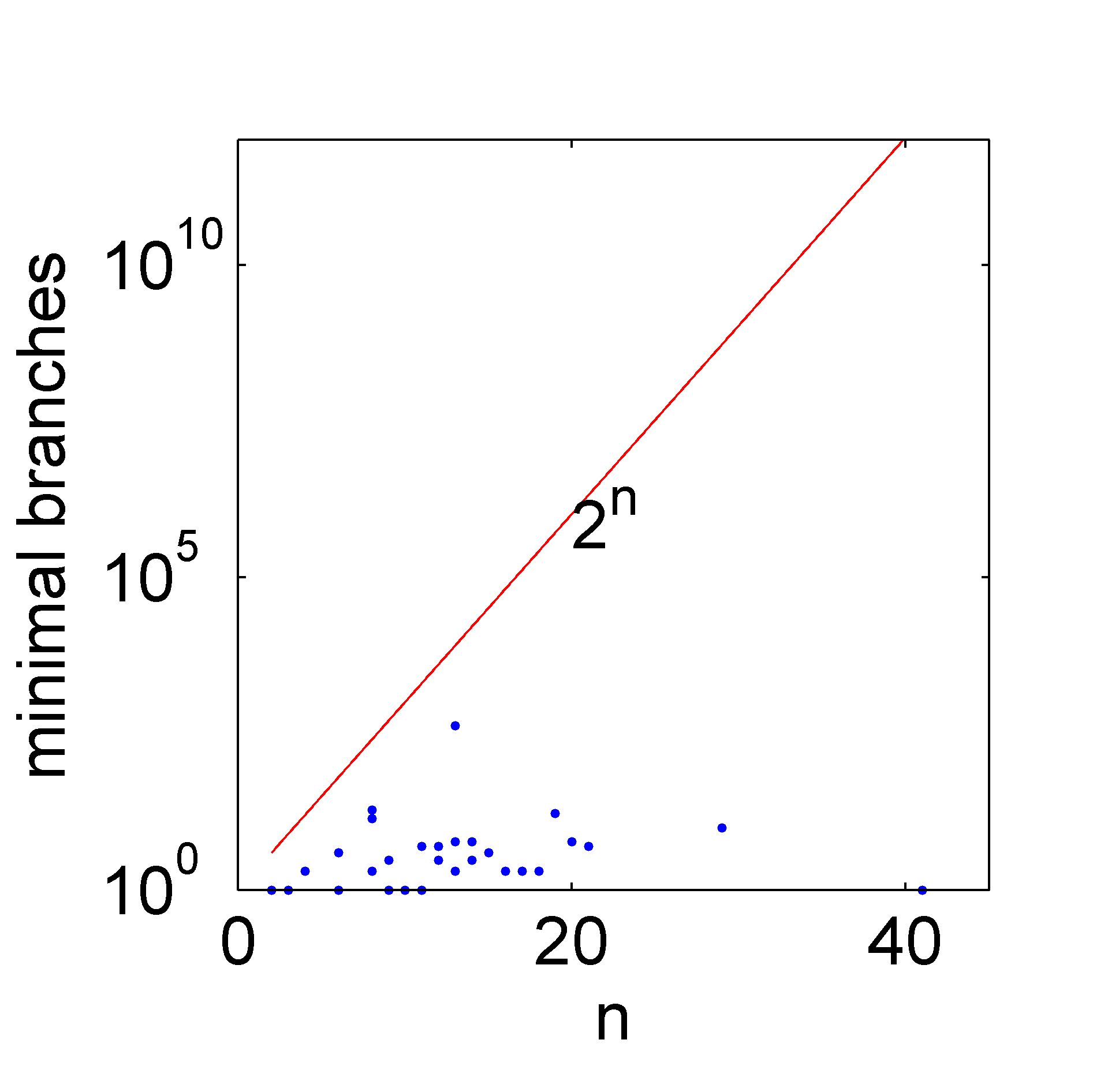
A summary of the analysis is presented in Table 1 with four different choices for $\varepsilon$ values (we wanted to have orders of magnitude close to decimal ones and to avoid commensurability between different values of $\varepsilon$; the choice $1/5$, $1/7$, $1/9$, $1/23$ seemed good enough for this purpose). In addition, in Fig. 2 we plot the number of minimal branches versus the number of equations in the model. As can be noticed, this number is much lower than the number of states of a boolean network with the same number of variables, which illustrates the advantage of our coarse graining with respect to boolean or multi-value networks.

Table 1: Summary of analysis on Biomodels database. The benchmarked models have a number of variables from 3 to 41. Model BIOMD0000000289 has tropical branches at $\varepsilon$ values $1/5$, $1/7$, $1/9$ but none at $1/23$. Model BIOMD0000000108 has no branches at all values of $\varepsilon$ considered for benchmarking.

$\varepsilon$ value	Total models considered	Models without tropical branches	Models with tropical branches	Average running time (in secs)	Average number of minimal branches
1/5	34	1	33	299.24	3.24
1/7	34	1	33	243.69	3
1/9	34	1	33	309.39	3.75
1/23	34	2	32	3178.21	3.84

Figure 2: Semi-log plot of the minimal branches versus the number of equations in the models from Biomodels for $\varepsilon=1/5$. Comparison with a binary network number of states $2^{n}$ suggests sub-exponential scaling.

4 Learning a finite state machine from a nonlinear biochemical network

In order to coarse grain the continuous model onto a finite-state automaton, we first need a way to map the phase space of the continuous model to a finite set of branches. First, we compute the branches of tropical solutions as subsets of the euclidian space ${\mathbb{R}}^{n}$ where $n$ is the number of variables. We are using the algorithm based on constraint solving introduced in [35] to obtain all rational tropical equilibration solutions $a=(a_{1},a_{2},\ldots,a_{n})$ within a box $|a_{i}|<b$, $b>0$ and with denominators smaller than a fixed value $d$, $a_{i}=p_{i}/q$, $p_{i},q$ are positive integers, $q<d$. The output of the algorithm is a matrix containing all the tropical equilibrations within the defined bounds. A post-processing treatment is applied to this output consisting in computing truncated systems, index sets, and minimal branches. Tropical equilibrations minimal branches are stored as matrices $A_{1},A_{2},\ldots,A_{b}$, whose lines are tropical solutions within the same branch. Here $b$ is the number of minimal branches.

Our method computes numerical approximations of the tropical prevariety. Given a value of $\epsilon$, this approximation is better when the denominator bound $d$ is high. At fixed $d$, the dependence of the precision on $\epsilon$ follows more intricate rules dictated by Diophantine approximations. For this reason, we systematically test that the number $b$ and the truncated systems corresponding to minimal branches are robust when changing the value of $\epsilon$.

Trajectories $x(t)=(x_{1}(t),\ldots,x_{n}(t))$ of the smooth dynamical system are generated with different initial conditions, chosen uniformly and satisfying the conservation laws, if any. For each time $t$, we compute the Euclidian distance $d_{i}(t)=\min_{y\in A_{i}}\left\lVert y-log_{\varepsilon}(x(t))\right\rVert,$ where $\left\lVert*\right\rVert$ denotes the Euclidean norm and $\log_{\varepsilon}(x)=(\log x_{1}/\log(\varepsilon),\ldots,\log x_{n}/\log(\varepsilon))$. This distance classifies all points of the trajectory as belonging to a tropical minimal branch. The result is a symbolic trajectory $s_{1},s_{2},\ldots$ where the symbols $s_{i}$ belong to the set of minimal branches. In order to include the possibility of transition regions we include an unique symbol $t$ to represent the situations when the minimal distance is larger than a fixed threshold. We also store the residence times $\tau_{1},\tau_{2},\ldots$ that represent the time spent in each of the state.

The stochastic automaton is learned as a homogenous, finite states, continuous time Markov process, defined by the lifetime (mean sojourn time) of each state $T_{i}$, $1\leq i\leq b$ and by the transition probabilities $p_{i,j}$ from a state $i$ to another state $j$. We use the following estimators for the lifetimes and for the transition probabilities:

$$T_{i} = (\sum_{n}\tau_{n}\mathonebb{1}_{s_{n}=i})/(\sum_{n}\mathonebb{1}_{s_{n}=i})$$ (15)

$$p_{i,j} = (\sum_{n}\mathonebb{1}_{s_{n}=i,s_{n+1}=j})/(\sum_{n}\mathonebb{1}_{s_{n}=i}),\,i\neq j$$ (16)

5 Application to TGF-$\beta$ signalling

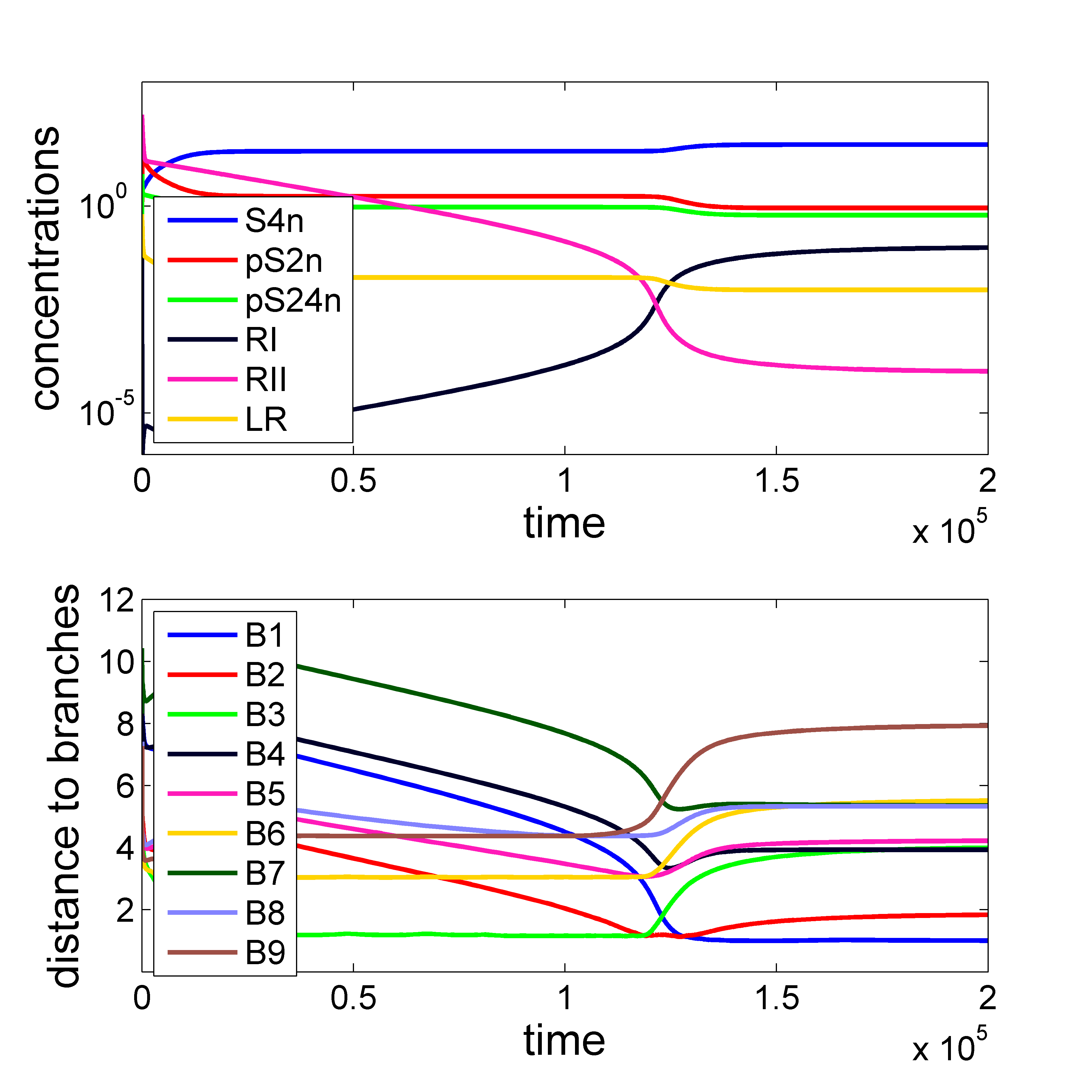
As a case study we consider a nonlinear model of dynamic regulation of Transforming Growth Factor beta TGF-$\beta$ signalling pathway that we have recently described in [1]. TGF-$\beta$ signalling occurs through association with a heteromeric complex of two types of transmembrane serine/threonine kinases, the type I (TGFBR1) and type II (TGFBR2) receptors. TGF-$\beta$ binding to TGFBR2 induces recruitment and phosphorylation of TGFBR1, which in turn transmits the signal through phosphorylation of Smad2 transcription factor. Once phosphorylated, the Smad2 hetero-dimerizes with Smad4 and the complexes then migrate to the nucleus, where they regulate the transcription of TGF-$\beta$-target genes. In that context, the Transcriptional Intermediary Factor 1, TIF1-$\gamma$ have been shown to function either as a transcriptional repressor or as an alternative transcription factor that promote TGF-$\beta$ signaling. The apparent controversial effect of TIF1-$\gamma$ on regulation of the Smad-dependent TGF-$\beta$ signalling was solved by a model integrating a ternary complex associating TIF1-$\gamma$ with Smad2 and Smad4 complexes. This model has a dynamics defined by $n=18$ polynomial differential equations and $25$ biochemical reactions. The computation of the tropical equilibrations for this model shows that there are 9 minimal branches of full equilibrations (in these tropical solutions all variables are equilibrated). The connectivity graph of these branches and the learned finite-state automaton are shown in Figure 3.

c)	d)

Figure 3: TGF$\beta$ model. a) Connectivity graph of tropical minimal branches; b) finite state automaton; c) a single trajectory of the system (starting from initial data chosen randomly close to the branch $B_{3}$) is represented by plotting the concentration of different species vs. time (upper sub-figure); the distances to different branches of solutions vs. time (lower sub-figure) shows that the sequence of branches for this trajectory is $B_{3}$, $B_{2}$, $B_{1}$ (all points of the trajectory are close to one of these three branches and significantly more distant to the other branches). d) The different branches of solutions are defined by allowed concentrations of different variables, represented here by orders of magnitudes $a_{i}$; the opposite concentration orders $-a_{i}$ are proportional to the logarithms of concentrations $-a_{i}\sim\log(x_{i})$. The most used branches are $B_{1}$, $B_{2}$, $B_{3}$ are shown in projection onto sets of three variables. The variables RI, RII, LR are plasma membrane receptors and ligand-receptor complex (signaling input layers), whereas pS2n, S4n, pS24n are nuclear transcription factors and complexes (effectors). The structure of tropical branches shows that composition of input layers is more flexible (varies on planar domains that are disjoint for different branches) than the concentrations of effectors (vary on linear intervals that overlap for different branches).

The transition probabilities of the automaton are coarse grained properties of the statistical ensemble of trajectories for different initial conditions. Given a state and a minimal branch close to it, it will depend on the actual trajectory to which other branch the system will be close to next. However, when initial data and the full trajectory are not known, the automaton will provide estimates of where we go next and with which probability. For the example studied and for nominal parameter values, the branch B1 is a globally attractive sink: starting from anywhere, the automaton will reach B1 with probability one. This branch contains the unique stable steady state of the initial model. This calculation illustrates the basic properties of minimal branches of equilibrations. Trajectories of the dynamical system can be decomposed into segments that remain close to minimal branches. Furthermore, all the observed transitions between branches are contained in the connectivity graph resulting from the polyhedral complex of the tropical equilibration branches. The connectivity graph can be thus used to constrain the possible transitions. A change of parameter values can have several consequences: change the connectivity graph, change of the probabilities of transitions and change of the attractor position.

In order to understand the significance of the minimal branches and their relation with dynamic and physiologic properties of the network we have performed an analytic study of the tropical equilibration solutions. We show in the following that the most important cause of the multiplicity of branches is the dynamics of the TGFBR1 and TGFBR2 receptors whose internalization and trafficking regulates TGF-$\beta$ signalling [13]. These two receptors belong to a ligand-receptor module of 6 variables and 12 reactions that is decoupled from the rest of the network. More precisely, the ligand-receptor module activates the SMAD transcription factors but receives no feed-back (see Figure 4) and can be studied independently from the rest of the variables. This module has been used with little variation in many models of TGF-$\beta$ signalling [38, 40, 4].

Full model

Reduced model

Figure 4: Graphic representation of the ligand-receptor module of the TGF-$\beta$ full model. A reduced model was found (see Appendix 2) that has the same tropical solutions as the full model and is used to simplify the calculation of the branches of tropical equilibrations. The different variables mean: $x_{12}:\,\text{RI}$ (TGBR1), $x_{13}:\,\text{RII}$ (TGFBR2), $x_{14}:\,\text{LR}$ (ligand-receptor complex), $x_{15}:\,\text{RIe}$ (TGFBR1 in endosome), $x_{16}:\,\text{RIIe}$ (TGFBR2 in endosome), $x_{11}:\,\text{LRe}$ (LR in endosome).

We show in the appendix 2 that the tropical equilibration of the ligand-receptor module form a two dimensional polyhedron conveniently parametrized by the concentration orders $a_{12}$ and $a_{13}$ of the receptors TGFBR1 and TGFBR2 respectively. The branches can be calculated analytically (Eqs.(24),(28)). For the nominal values of the model parameters one of these branches is empty and the three remaining branches correspond to $B_{1}$, $B_{2}$ and $B_{3}$. The two other triplets of branches $(B_{4},B_{5},B_{6})$ and $(B_{7},B_{8},B_{9})$ correspond to the same mutual relations of variables in the ligand-receptor module. They are distinguished by the values of the remaining variables (the transcription factors module). Our computation of the automaton showed that the branches $B_{i},\,i\in[4,9]$ are practically inaccessible from states in branches $B_{i},\,\,i\in[1,3]$, therefore we will not discuss them here.

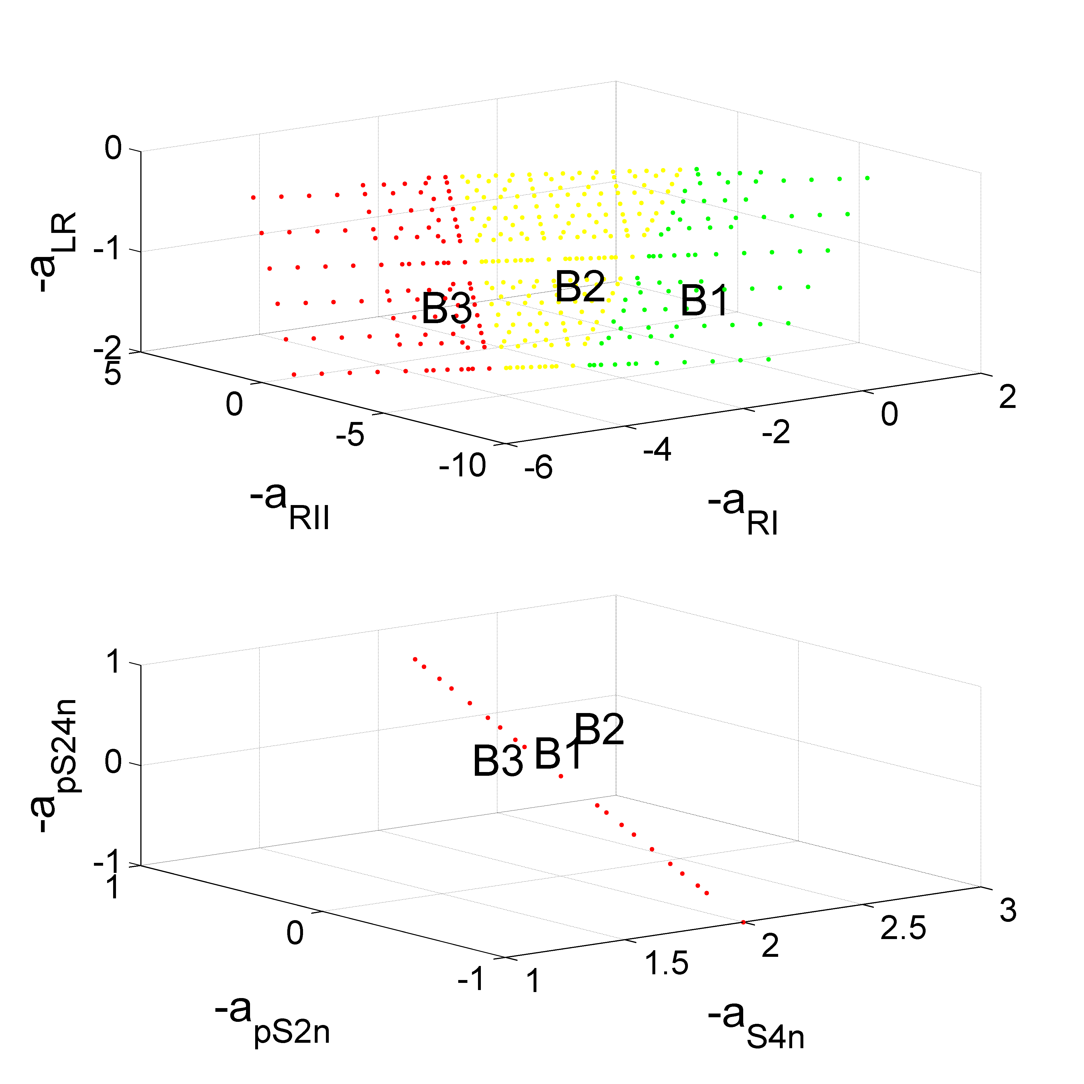
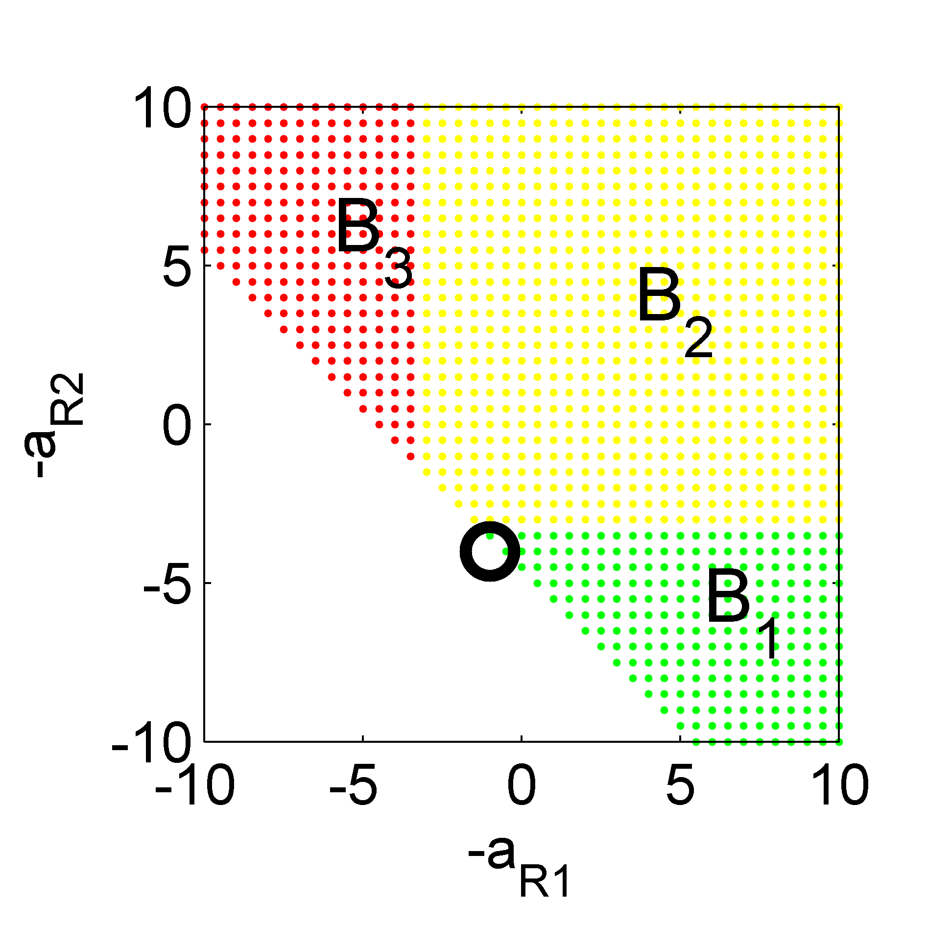
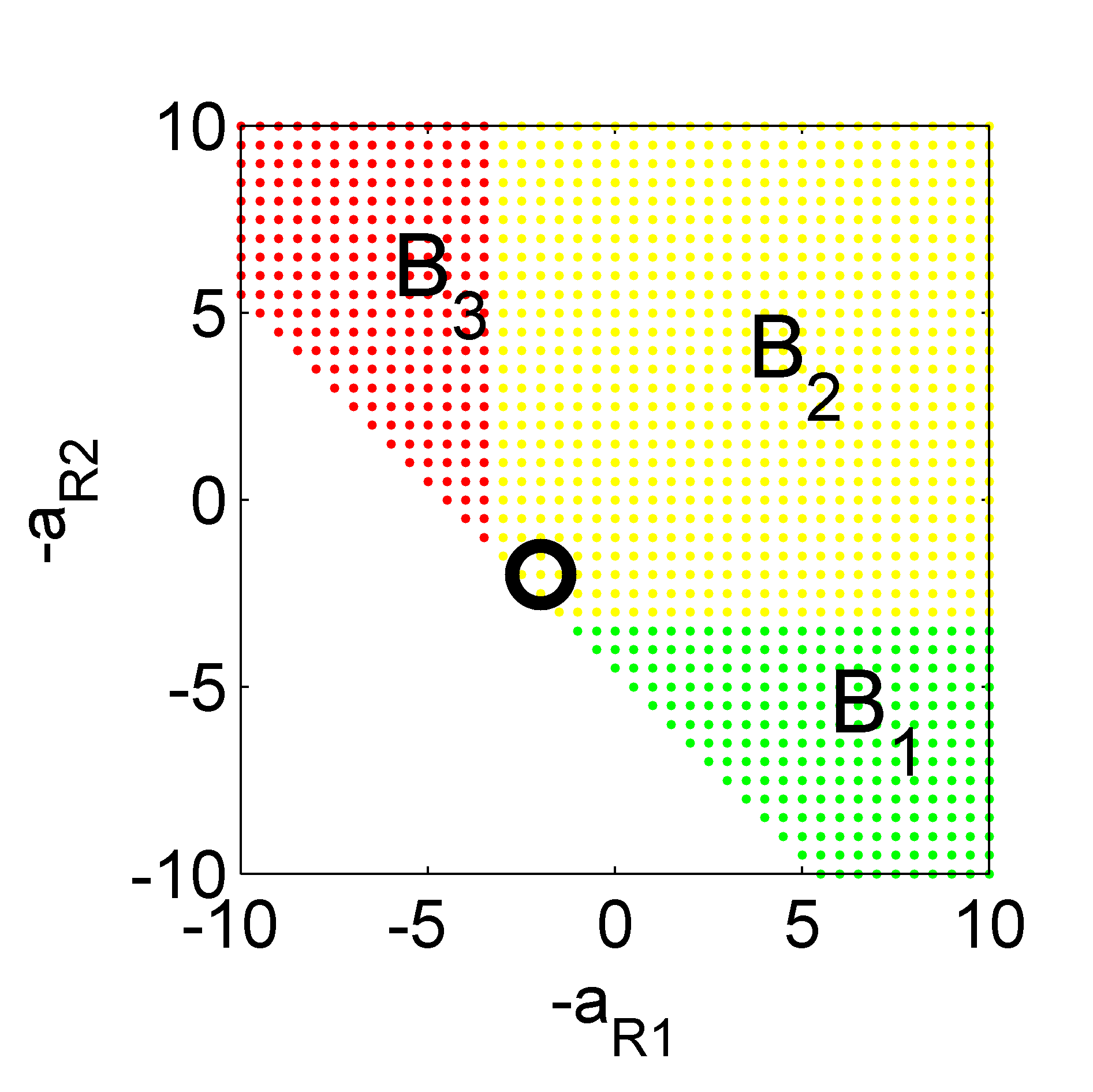
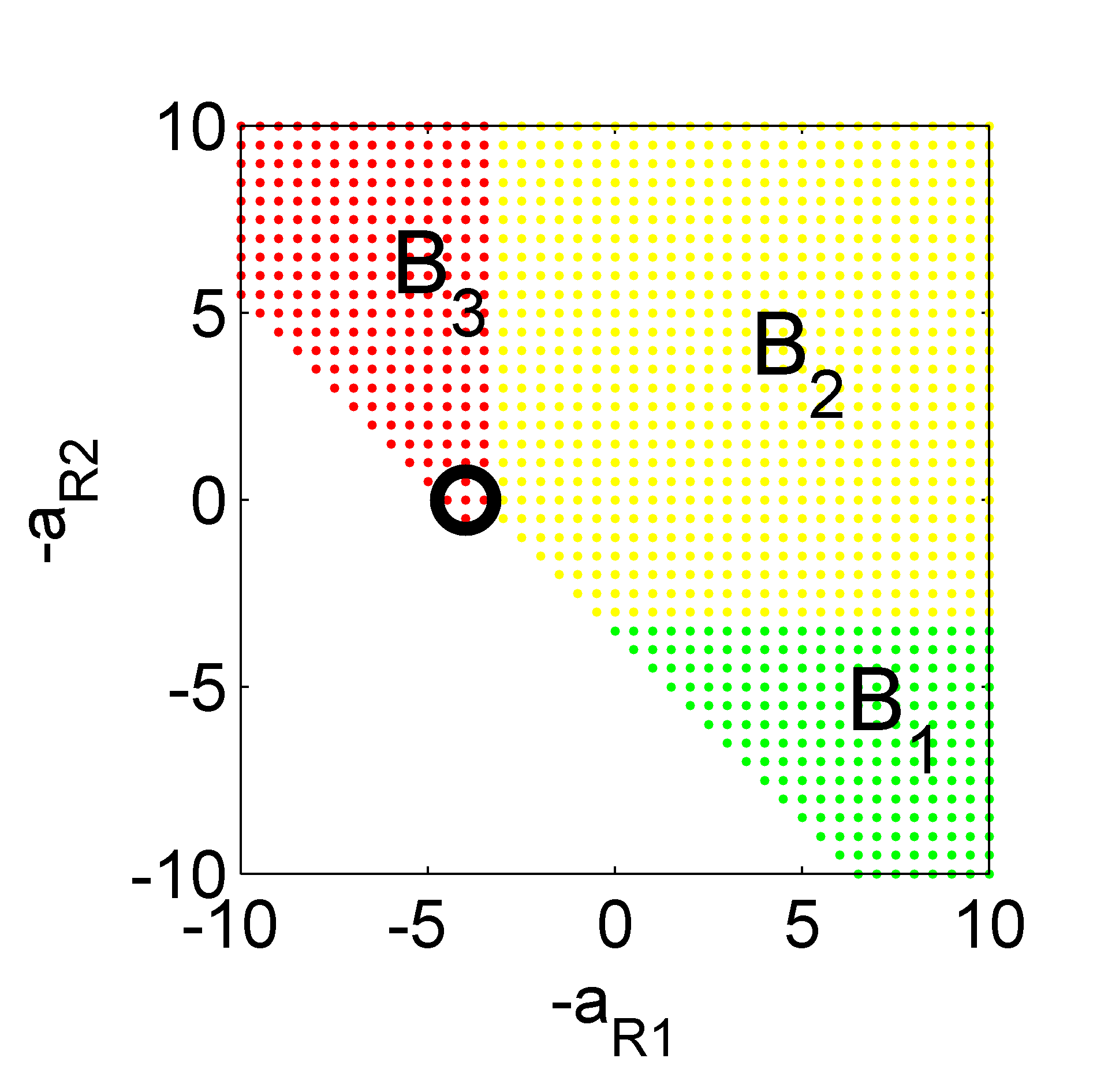
We have used symbolic computation to determine the steady states of the ligand-receptor module. This module has an unique steady state corresponding to concentrations orders that can be placed inside the polyhedron of tropical solutions using the Eq.(3). The minimal branch containing the steady state is a sink of the coarse grained dynamics. The polyhedron of tropical solutions, its decomposition into minimal branches, and the position of the steady states inside it, depend on model parameters. Among model parameters two are important: $k_{18}$ and $k_{19}$ representing the production rate of the protein receptors TGFBR1 and TGFBR2, respectively. Consequently, these two parameters are correlated to gene expression and account for possible variability in mRNA levels of the two types of receptors. Figure 5 shows the tropical equilibration branches of the ligand-receptor modules for various parameters $k_{19}$ corresponding to various TGFBR2 expression levels. For the nominal parameters used in the model, the branch $B1$ is an attractor (the coarse-grained dynamics shows that the probability to leave this state is negligible), and the branches $B2$ and $B3$ are only metastable. This means that starting in the branch $B2$ or $B3$ the receptor module will reach the branch $B1$ after a certain time and will remain there. However, over-expression of TGFBR2 modelled by changing the parameter $k_{19}$ and illustrated in the Figure 5a-c can tilt the balance in favor of large concentrations of receptor of type 2 corresponding to branches $B2$, $B3$ of tropical solutions in the model. Interestingly, this change occurs by a displacement of the position of the steady state from $B1$ to $B2$ and $B3$ and not by a change of the concentration values allowed for these branches.

a)	b)
c)	d)

Figure 5: Tropical equilibrations of the ligand-receptor modules for various values of TGFBR2 (R2) gene expression are represented in projection in the plane $(a_{R1},a_{R2})$ (a point in this plane provides the orders of concentrations of the protein receptors) (a,b, and c) and comparison with proteomics data from [5] (d). Branches of tropical equilibrations are calculated for a) nominal value $k_{19}$ (TGFBR2 expression) (this is the same as Fig.4d in projection onto the plane $(a_{R1},a_{R2})$), b) $\times 2$ TGFBR2 overexpression , and c) $\times 10$ TGFBR2 overexpression. The circle represents the position of the stable steady state and the branch containing is an attractor of the finite-state automaton. d) Proteomic data from NCI-60 cancer cell lines. Aggressive lines cover concentration domains corresponding to branches 3 and 2, whereas non-aggressive lines correspond to low expression of TGFBR2 in branch 1.

While Vilar et al [38] have speculated that the ligand-receptor module is responsible for the versatility of the response of the TGF-$\beta$ pathway, no experimental evidence support this hypothesis. Here, we now demonstrate that there are correlations between dynamical specificity characterized by membership to a particular branch of equilibration and cell phenotype. We illustrate such a comparison for the NCI-60 panel of cancer cell lines, a well established tool for tumour comparison and drug screening provided by the National Cancer Institute. Based on microarray analysis, these cell lines were found to cluster into two classes: epithelium-like (non-aggressive) and mesenchymal-like (aggressive) cell lines [27].

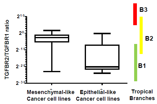
Using the global proteome analysis of this NCI-60 panel [5] we extracted the protein expression levels of TGFBR1 and TGFBR2 and showed that mesenchymal-like (aggressive) cell lines can be distinguished from epithelial-like (non-aggressive) cell lines by the increased level of TGFBR2 (Fig 5d.

The proteome data was compared to membership to tropical branches. According to Eq.(3) there is a linear relation between opposite concentration orders $-a_{i}$ and logarithms of concentrations, $-a_{i}\approx b\log(x_{i}),\,i=1,\ldots,n$ ($b=-1/\log(\varepsilon)>0$). We used opposite concentration orders $-a_{i}$ instead of $a_{i}$ because they change in the same direction as the concentrations (small opposite orders mean small concentrations and large opposite orders mean large concentrations). Therefore, in Fig 5a-c the relation $TGFBR1=TGFBR2$ is verified on the bissector of the first quadrant, whereas $TGFBR2>TGFBR1$ and $TGFBR2<TGFBR1$ are valid above and below the bissector, respectively. When compared the proteome results with the membership to a particular branch of equilibration, we found that the distribution of concentration orders in branches place non-aggressive cancer cell lines in a range covered by branch 1, whereas the aggressive cancer cell lines are placed in a range covered by branches 2 and 3 (Fig 5d. Indeed, the ratio $TGFBR2/TGFBR1$ is small for the branch $B_{1}$ and in non-aggressive cancer cell lines, and is much larger for $B_{2},B_{3}$ and in aggressive cell lines.

Furthermore, we validated the association of up-regulation of TGFBR2 with mesenchymal-like appearance in an independent dataset of 51 breast cancer cell lines [19]. As we have recently described [28], comparative analyses between Basal B cell lines with mesenchymal-like phenotype and Basal A and Luminal cell lines with epithelial morphology permitted to identify more than 600 differentially expressed genes that include TGFBR2. Gene expression data were now extracted for TGFBR1 and TGFBR2 and we showed that TGFBR2 gene expression is significantly induced in mesenchymal-like cell lines while TGFBR1 did not vary (Supplementary Figure 1). In accordance with our observation, Parker et al. [23] have previously reported the association of low TGFBR2 expression with a lower aggressive tumour phenotype.

In the present work, our tropical approach has identified TGFBR2 concentration as a discriminant parameter for defining metastable regimes. The importance of such up-regulation of TGFBR2 in aggressive cancer cell lines might be related to its implication in Smad-independent signaling that includes PI3K-Akt, JNK, p38MAPK and Rho-like GTPases and which highly contribute to epithelial-mesenchymal transition [39, 18].

Together these observations suggest that metastable regimes defined by branches of minimal tropical equilibrations are associated with cell phenotypes. The idea of associating tropical minimal branches with clinical phenotype is similar to the idea of cancer attractors [11] where the idea is that cancer cells are trapped in some abnormal attractors.

6 Conclusion

We have presented a method to coarse grain the dynamics of a smooth biochemical reaction network to a discrete symbolic dynamics of a finite state automaton. The coarse graining was obtained using a tropical geometry approach to compute the states. These states correspond to metastable dynamic regimes and to relatively slow segments of the system trajectories. The coarse grained model can be used for studying statistical properties of biochemical networks such as occurrence and stability of temporal patterns, recurrence, periodicity and attainability problems.

Further improvement and evolution is possible for this approach. First, the coarse graining can be performed in a hierarchical way. For the nonlinear example studied in the paper we computed only the full tropical equilibrations that stand for the lowest order in the hierarchy (coarsest model). As discussed in Section 3 we can also consider partial equilibrations when slow variables are not equilibrated and thus refine the automaton. Generally, there are more partial equilibrations than total equilibrations and learning an automaton on the augmented state set will produce refinements. Second, and most importantly, the dynamics within a branch could be also described. As shown elsewhere, reductions of the systems of ordinary equations are valid locally close to tropical equilibrations [20, 21, 26, 30]. Furthermore, the same reduction is valid for all the equilibrations in a branch. This suggests that a hybrid approach, combining reduced ODE dynamics within branch with discrete transitions between branches is feasible. The transitions can be autonomously and deterministically commanded by crossing the boundaries between branches that are perfectly determined by our approach.

The most important result of this paper is the extension of the notion of attractor to metastable regimes of chemical reaction networks and the proposition of a practical recipe to compute metastability. Metastable regimes correspond to low-dimensional hypersurfaces of the phase space, along which the dynamics is relatively slower. Most likely, metastable regimes have biological importance because the network spends most of its time in these states. The itinerancy of the network, described as the possibility of transitions from one metastable regime to another is paramount to the way neural networks compute, retrieve and use information [37] and can have similar role in biochemical networks. Our approach based on tropical geometry provides an algorithmic method to test these ideas further. The extension of this approach i.e. making use of statistical methods to compute the association of the tropical minimal branches with clinical phenotypes based on “-omics” data remains a topic of future research.

Acknowledgements

O.R and A.N are supported by INCa/Plan Cancer grant N^∘ASC14021FSA.

Appendix 1: Description of the TGFb model used in this paper.

The model is described by the following system of differential equations

$$\frac{\mathrm{d}x_{1}}{\mathrm{d}t} = k_{2}x_{2}-k_{1}x_{1}-k_{16}x_{1}x_{11}$$

$$\frac{\mathrm{d}x_{2}}{\mathrm{d}t} = k_{1}x_{1}-k_{2}x_{2}+k_{17}k_{34}x_{6}$$

$$\frac{\mathrm{d}x_{3}}{\mathrm{d}t} = k_{3}x_{4}-k_{3}x_{3}+k_{7}x_{7}+k_{33}k_{37}x_{18}-k_{6}x_{3}x_{5}$$

$$\frac{\mathrm{d}x_{4}}{\mathrm{d}t} = k_{3}x_{3}-k_{3}x_{4}+k_{9}x_{8}-k_{8}x_{4}x_{6}$$

$$\frac{\mathrm{d}x_{5}}{\mathrm{d}t} = k_{5}x_{6}-k_{4}x_{5}+k_{7}x_{7}+2k_{11}x_{9}-2k_{10}x_{5}^{2}-k_{6}x_{3}x_{5}+k_{16}x_{1}x_{11}$$

$$\frac{\mathrm{d}x_{6}}{\mathrm{d}t} = k_{4}x_{5}-k_{5}x_{6}+k_{9}x_{8}+2k_{13}x_{10}-2k_{12}x_{6}^{2}-k_{17}k_{34}x_{6}+k_{31}k_{36}x_{8}-k_{8}x_{4}x_{6}$$

$$\frac{\mathrm{d}x_{7}}{\mathrm{d}t} = k_{6}x_{3}x_{5}-x_{7}(k_{7}+k_{14})$$

$$\frac{\mathrm{d}x_{8}}{\mathrm{d}t} = k_{14}x_{7}-k_{9}x_{8}-k_{31}k_{36}x_{8}+k_{8}x_{4}x_{6}$$

$$\frac{\mathrm{d}x_{9}}{\mathrm{d}t} = k_{10}x_{5}^{2}-x_{9}(k_{11}+k_{15})$$

$$\frac{\mathrm{d}x_{10}}{\mathrm{d}t} = k_{15}x_{9}-k_{13}x_{10}+k_{12}x_{6}^{2}$$

$$\frac{\mathrm{d}x_{11}}{\mathrm{d}t} = k_{23}x_{14}-k_{30}x_{11}$$

$$\frac{\mathrm{d}x_{12}}{\mathrm{d}t} = k_{18}-x_{12}(k_{20}+k_{26})+k_{30}x_{11}+k_{27}x_{15}-k_{22}k_{35}x_{12}x_{13}$$

$$\frac{\mathrm{d}x_{13}}{\mathrm{d}t} = k_{19}-x_{13}(k_{21}+k_{28})+k_{30}x_{11}+k_{29}x_{16}-k_{22}k_{35}x_{12}x_{13}$$

$$\frac{\mathrm{d}x_{14}}{\mathrm{d}t} = k_{22}k_{35}x_{12}x_{13}-x_{14}(k_{23}+k_{24}+k_{25})$$

$$\frac{\mathrm{d}x_{15}}{\mathrm{d}t} = k_{26}x_{12}-k_{27}x_{15}$$

$$\frac{\mathrm{d}x_{16}}{\mathrm{d}t} = k_{28}x_{13}-k_{29}x_{16}$$

$$\frac{\mathrm{d}x_{17}}{\mathrm{d}t} = k_{31}k_{36}x_{8}-k_{32}x_{17}$$

$$\frac{\mathrm{d}x_{18}}{\mathrm{d}t} = k_{32}x_{17}-k_{33}k_{37}x_{18}$$ (17)

These variables are as follows:

• Receptors on plasma membrane: $x_{12}=$ RI (receptor 1), $x_{13}=$ RII (receptor 2), $x_{14}=$ LR (ligand-receptor complex).

• Receptors in the endosome: $x_{11}=$ LRe, $x_{15}=$ RIe, $x_{16}=$ RIIe.

• Transcription factors and complexes in cytosol: $x_{1}=$ S2c, $x_{3}=$ S4c, $x_{5}=$ pS2c, $x_{7}=$ pS24c, $x_{9}=$ pS22c, $x_{18}=$ S4ubc.

• Transcription factors and complexes in the nucleus: $x_{2}=$ S2n, $x_{4}=$ S4n, $x_{6}=$ pS2n, $x_{8}=$ pS24n, $x_{10}=$ pS22n, $x_{17}=$ S4ubn.

Appendix 2: Calculation of tropical equilibration branches for the TGFb model used in this paper.

Tropical equilibration solutions for the variables $x_{11}$,$x_{12}$, $x_{13}$, $x_{14}$, $x_{15}$, $x_{16}$ can be computed independently from the rest of the variables. The ordinary differential equations for these variables form a subsystem that is decoupled (receives no feed-back) from the rest of the equations.

We can reduce the system of 6 tropical equations to a simplified system of 3 tropical equations using the following two general properties.

Property 6.1 (binomial species)

$Y$ is a binomial species if the ordinary differential equation defining its rate of variation contains only one positive monomial term and only one negative monomial term

$$\frac{\mathrm{d}Y}{\mathrm{d}t}=M_{1}(X)Y^{n_{1}}-M_{2}(X)Y^{n_{2}},$$

where $X$ denotes the other variables. We further assume that $n_{1}<n_{2}$. Then, the species $Y$ can be eliminated and the resulting simplified tropical system has the same tropical equilibration solutions as the full system. The simplification is performed by eliminating the equation for $Y$ and replacing everywhere $Y$ by $(M_{1}/M_{2})^{1/(n_{2}-n_{1})}$.

The proof follows from the fact that the tropical equation for the order $a$ of $Y$ is linear in $a$ (there is no min operation) and therefore it has the unique solution $a=\frac{1}{(n_{2}-n_{1})}(\mu_{1}-\mu_{2})$.

Property 6.2 (dominated first order reactions)

If a species $Y$ is consumed by several first order reactions of kinetic constants $k_{1},k_{2},\ldots,k_{r}$ and if $\gamma_{1}\leq\gamma_{2}\leq\ldots\leq\gamma_{p}<\gamma_{p+1}\leq\gamma_{p+2}\leq\ldots\leq\gamma_{r}$, then the reactions $k_{p+1},\ldots,k_{r}$ can be eliminated and the resulting simplified tropical system has the same tropical equilibration solutions as the full system.

The proof follows from the following obvious property of the min operation $\min(\gamma_{1},\ldots,\gamma_{p},\ldots,\gamma_{r})=\min(\gamma_{1},\ldots,\gamma_{p})$.

Using $\gamma_{26}<\gamma_{20}$, $\gamma_{28}<\gamma_{21}$ (a condition satisfied by the nominal model parameters and meaning that internalization is more rapid than degradation for both receptors 1 and 2) and the Properties 6.1,6.2 we can justify the reduction illustrated in Figure 4. Because the reduced model has the same tropical solutions as the full, larger model, it is enough to solve the tropical equilibration problem for the reduced model. This reads

$$\min(\gamma_{18},a_{14}+\gamma_{23},a_{12}+\gamma_{26}) = \min(a_{12}+a_{13}+\gamma_{22}+\gamma_{35},a_{12}+\gamma_{26})$$ (18)

$$\min(\gamma_{19},a_{14}+\gamma_{23},a_{13}+\gamma_{28}) = \min(a_{12}+a_{13}+\gamma_{22}+\gamma_{35},\gamma_{28}+a_{13})$$ (19)

$$\min(\gamma_{24},\gamma_{25},\gamma_{23})+a_{14} = a_{12}+a_{13}+\gamma_{22}+\gamma_{35}$$ (20)

Suppose now that the following condition is true

$$\min(\gamma_{24},\gamma_{25},\gamma_{23})=\gamma_{23}.$$ (21)

This condition is satisfied by the nominal parameters and, like the previous condition, means that receptors have relatively large life-times. Then from (20) we got $a_{14}=a_{12}+a_{13}+\gamma_{22}+\gamma_{35}-\gamma_{23}$ and the equations (18),(19) become

$$\min(\gamma_{18},a_{14}+\gamma_{23},a_{12}+\gamma_{26}) = \min(a_{14}+\gamma_{23},a_{12}+\gamma_{26})$$ (22)

$$\min(\gamma_{19},a_{14}+\gamma_{23},a_{13}+\gamma_{28}) = \min(a_{14}+\gamma_{23},a_{13}+\gamma_{28})$$ (23)

The solutions of (22), (23) can be easily found and form the following polyhedron

$$(\{a_{12}+a_{13}+\gamma_{22}+\gamma_{35}\leq\gamma_{18}\} \cup \{\gamma_{26}+a_{12}\leq\gamma_{18}\})\cap$$

$$(\{a_{12}+a_{13}+\gamma_{22}+\gamma_{35}\leq\gamma_{19}\} \cup \{\gamma_{28}+a_{13}\leq\gamma_{19}\}),$$

$$a_{14} = a_{12}+a_{13}+\gamma_{22}+\gamma_{35}-\gamma_{23}.$$ (24)

The orders of the remaining variables can be found as indicated in Prop.6.1:

$$a_{15} = a_{12}+\gamma_{26}-\gamma_{27},$$ (25)

$$a_{16} = a_{13}+\gamma_{28}-\gamma_{29},$$ (26)

$$a_{11} = a_{12}+a_{13}+\gamma_{22}+\gamma_{35}-\gamma_{30}.$$ (27)

The polyhedron of tropical solutions defined by Eq.(24) can be partitioned into minimal branches (also polyhedra). This can be done by checking which term is dominant in the ordinary differential equations for the variables $x_{12}$, $x_{13}$ and $x_{14}$ (see Eqs.(17)). The result is that there are at most four minimal branches defined by one of the conditions

$$\{a_{12}+\gamma_{26}<a_{12}+a_{13}+\gamma_{22}+\gamma_{35}\}\cap\{a_{13}+\gamma_{28}<a_{12}+a_{13}+\gamma_{22}+\gamma_{35}\}$$

$$\{a_{12}+\gamma_{26}<a_{12}+a_{13}+\gamma_{22}+\gamma_{35}\}\cap\{a_{13}+\gamma_{28}>a_{12}+a_{13}+\gamma_{22}+\gamma_{35}\}$$

$$\{a_{12}+\gamma_{26}>a_{12}+a_{13}+\gamma_{22}+\gamma_{35}\}\cap\{a_{13}+\gamma_{28}<a_{12}+a_{13}+\gamma_{22}+\gamma_{35}\}$$

$$\{a_{12}+\gamma_{26}>a_{12}+a_{13}+\gamma_{22}+\gamma_{35}\}\cap\{a_{13}+\gamma_{28}>a_{12}+a_{13}+\gamma_{22}+\gamma_{35}\}$$ (28)

References

- [1] Geoffroy Andrieux, Laurent Fattet, Michel Le Borgne, Ruth Rimokh, and Nathalie Théret. Dynamic regulation of Tgf-B signaling by Tif1: a computational approach. PloS one, 7(3):e33761, 2012.
- [2] Cheng-Shang Chang. On deterministic traffic regulation and service guarantees: a systematic approach by filtering. IEEE Transactions on Information Theory, 44(3):1097–1110, 1998.
- [3] Eliodoro Chiavazzo and Ilya Karlin. Adaptive simplification of complex multiscale systems. Physical Review E, 83(3):036706, 2011.
- [4] Seung-Wook Chung, Fayth L Miles, Robert A Sikes, Carlton R Cooper, Mary C Farach-Carson, and Babatunde A Ogunnaike. Quantitative modeling and analysis of the transforming growth factor signaling pathway. Biophysical journal, 96(5):1733–1750, 2009.
- [5] Amin Moghaddas Gholami, Hannes Hahne, Zhixiang Wu, Florian Johann Auer, Chen Meng, Mathias Wilhelm, and Bernhard Kuster. Global proteome analysis of the nci-60 cell line panel. Cell reports, 4(3):609–620, 2013.
- [6] A. N. Gorban and O. Radulescu. Dynamic and static limitation in reaction networks, revisited. In David West Guy B. Marin and Gregory S. Yablonsky, editors, Advances in Chemical Engineering – Mathematics in Chemical Kinetics and Engineering, volume 34 of Advances in Chemical Engineering, pages 103–173. Elsevier, 2008.
- [7] Alexander N. Gorban, Ovidiu Radulescu, and Andrei Y. Zinovyev. Asymptotology of chemical reaction networks. Chemical Engineering Science, 65(7):2310–2324, 2010.
- [8] Alexander N Gorban and Muhammad Shahzad. The Michaelis-Menten-Stueckelberg theorem. Entropy, 13(5):966–1019, 2011.
- [9] A.N. Gorban and I.V. Karlin. Invariant manifolds for physical and chemical kinetics, volume 660 of Lect. Notes Phys. Springer, 2005.
- [10] George Haller and Themistoklis Sapsis. Localized instability and attraction along invariant manifolds. SIAM Journal on Applied Dynamical Systems, 9(2):611–633, 2010.
- [11] Huang, Sui and Ernberg, Ingemar and Kauffman, Stuart. Cancer attractors: A systems view of tumors from a gene network dynamics and developmental perspective. Seminars in Cell Developmental Biology , 20(7):869 – 876, 2009.
- [12] Nicolas Le Novere, Benjamin Bornstein, Alexander Broicher, Melanie Courtot, Marco Donizelli, Harish Dharuri, Lu Li, Herbert Sauro, Maria Schilstra, Bruce Shapiro, Jacky L. Snoep, and Michael Hucka. BioModels database: a free, centralized database of curated, published, quantitative kinetic models of biochemical and cellular systems. Nucleic Acids Research, 34(suppl 1):D689–D691, 2006.
- [13] Christine Le Roy and Jeffrey L Wrana. Clathrin-and non-clathrin-mediated endocytic regulation of cell signalling. Nature reviews Molecular cell biology, 6(2):112–126, 2005.
- [14] GL Litvinov. Maslov dequantization, idempotent and tropical mathematics: a brief introduction. Journal of Mathematical Sciences, 140(3):426–444, 2007.
- [15] Ulrich Maas and Stephen B Pope. Simplifying chemical kinetics: intrinsic low-dimensional manifolds in composition space. Combustion and Flame, 88(3):239–264, 1992.
- [16] Diane Maclagan and Bernd Sturmfels. Introduction to tropical geometry, volume 161 of Graduate Studies in Mathematics. American Mathematical Society, RI, 2015.
- [17] Wolfgang Meiske. An approximate solution of the michaelis-menten mechanism for quasi-steady and state quasi-equilibrium. Mathematical Biosciences, 42(1):63–71, 1978.
- [18] Aristidis Moustakas and Carl-Henrik Heldin. Induction of epithelial–mesenchymal transition by transforming growth factor . In Seminars in cancer biology, volume 22, pages 446–454. Elsevier, 2012.
- [19] Richard M Neve, Koei Chin, Jane Fridlyand, Jennifer Yeh, Frederick L Baehner, Tea Fevr, Laura Clark, Nora Bayani, Jean-Philippe Coppe, Frances Tong, et al. A collection of breast cancer cell lines for the study of functionally distinct cancer subtypes. Cancer cell, 10(6):515–527, 2006.
- [20] Vincent Noel, Dima Grigoriev, Sergei Vakulenko, and Ovidiu Radulescu. Tropical geometries and dynamics of biochemical networks application to hybrid cell cycle models. In Jérôme Feret and Andre Levchenko, editors, Proceedings of the 2nd International Workshop on Static Analysis and Systems Biology (SASB 2011), volume 284 of Electronic Notes in Theoretical Computer Science, pages 75–91. Elsevier, 2012.
- [21] Vincent Noel, Dima Grigoriev, Sergei Vakulenko, and Ovidiu Radulescu. Tropicalization and tropical equilibration of chemical reactions. In G Litvinov and S Sergeev, editors, Tropical and Idempotent Mathematics and Applications, volume 616 of Contemporary Mathematics, pages 261–277. American Mathematical Society, 2014.
- [22] L. Pachter and B. Sturmfels. Tropical geometry of statistical models. Proceedings of the National Academy of Sciences of the United States of America, 101(46):16132, 2004.
- [23] Alexander Scott Parker, Christine M Lohse, Kevin Wu, Pamela Kreinest, John A Copland, Tracy Hilton, Michael Wehle, John C Cheville, and Michael Blute. Lower expression levels of the transforming growth factor beta receptor type ii protein are associated with a less aggressive tumor phenotype and improved survival among patients with clear cell renal cell carcinoma. Human pathology, 38(3):453–461, 2007.
- [24] Mikhail I Rabinovich, Valentin S Afraimovich, Christian Bick, and Pablo Varona. Information flow dynamics in the brain. Physics of life reviews, 9(1):51–73, 2012.
- [25] Mikhail I Rabinovich, Pablo Varona, Allen I Selverston, and Henry DI Abarbanel. Dynamical principles in neuroscience. Reviews of modern physics, 78(4):1213, 2006.
- [26] Ovidiu Radulescu, Sergei Vakulenko, and Dima Grigoriev. Model reduction of biochemical reactions networks by tropical analysis methods. Mathematical Model of Natural Phenomena, 10(3):124–138, 2015.
- [27] Douglas T Ross, Uwe Scherf, Michael B Eisen, Charles M Perou, Christian Rees, Paul Spellman, Vishwanath Iyer, Stefanie S Jeffrey, Matt Van de Rijn, Mark Waltham, et al. Systematic variation in gene expression patterns in human cancer cell lines. Nature genetics, 24(3):227–235, 2000.
- [28] Michaël Ruff, Anthony Leyme, Fabienne Le Cann, Dominique Bonnier, Jacques Le Seyec, Franck Chesnel, Laurent Fattet, Ruth Rimokh, Georges Baffet, and Nathalie Théret. The disintegrin and metalloprotease adam12 is associated with tgf--induced epithelial to mesenchymal transition. PloS one, 10(9):e0139179, 2015.
- [29] Satya Swarup Samal, Dima Grigoriev, Holger Fröhlich, and Ovidiu Radulescu. Analysis of reaction network systems using tropical geometry. In Vladimir P. Gerdt, Wolfram Koepf, Werner M. Seiler, and Evgenii V. Vorozhtsov, editors, Computer Algebra in Scientific Computing – 17th International Workshop (CASC 2015), volume 9301 of Lecture Notes in Computer Science, pages 422–437, Aachen, Germany, September 2015. Springer.
- [30] Satya Swarup Samal, Dima Grigoriev, Holger Fröhlich, Andreas Weber, and Ovidiu Radulescu. A geometric method for model reduction of biochemical networks with polynomial rate functions. arXiv preprint arXiv:1510.04716, Bulletin of Mathematical Biology, in press., 2015.
- [31] Satya Swarup Samal, Ovidiu Radulescu, Dima Grigoriev, Holger Fröhlich, and Andreas Weber. A tropical method based on newton polygon approach for algebraic analysis of biochemical reaction networks. In 9th European Conference on Mathematical and Theoretical Biology, 2014.
- [32] Lee A Segel. On the validity of the steady state assumption of enzyme kinetics. Bulletin of Mathematical Biology, 50(6):579–593, 1988.
- [33] Lee A Segel and Marshall Slemrod. The quasi-steady-state assumption: a case study in perturbation. SIAM Review, 31(3):446–477, 1989.
- [34] Imre Simon. Recognizable sets with multiplicities in the tropical semiring. In Mathematical Foundations of Computer Science 1988, pages 107–120. Springer, 1988.
- [35] Sylvain Soliman, François Fages, and Ovidiu Radulescu. A constraint solving approach to model reduction by tropical equilibration. Algorithms for Molecular Biology, 9(1):24, 2014.
- [36] Thorsten Theobald. On the frontiers of polynomial computations in tropical geometry. Journal of Symbolic Computation, 41(12):1360–1375, 2006.
- [37] Ichiro Tsuda. Chaotic itinerancy as a dynamical basis of hermeneutics in brain and mind. World Futures: Journal of General Evolution, 32(2-3):167–184, 1991.
- [38] JM Vilar, Ronald Jansen, and Chris Sander. Signal processing in the tgf-beta superfamily ligand-receptor network. PLoS Comput Biol, 2(1):e3, 2006.
- [39] Ying E Zhang. Non-smad pathways in tgf- signaling. Cell research, 19(1):128–139, 2009.
- [40] Zhike Zi and Edda Klipp. Constraint-based modeling and kinetic analysis of the smad dependent tgf-beta signaling pathway. PLoS One, 2(9):e936–e936, 2007.