TIF-UNIMI-2015-18

We derive a general resummation formula for transverse-momentum distributions of hard processes at the leading logarithmic level in the high-energy limit, to all orders in the strong coupling. Our result is based on a suitable generalization of high-energy factorization theorems, whereby all-order resummation is reduced to the determination of the Born-level process but with incoming off-shell gluons. We validate our formula by applying it to Higgs production in gluon fusion in the infinite top mass limit. We check our result up to next-to-leading order by comparison to the high energy limit of the exact expression and to next-to-next-to leading order by comparison to NNLL transverse momentum (Sudakov) resummation, and we predict the high-energy behaviour at next³-to-leading order. We also show that the structure of the result in the small transverse momentum limit agrees to all orders with general constraints from Sudakov resummation.

1 High-energy factorization

High-energy resummation allows the computations of contributions to hard QCD processes, to all orders in the strong coupling $\alpha_{s}$, which are enhanced by powers of logs of the ratio $1/x$ of the center-of-mass energy $s$ to the scale of the hard process $Q^{2}$: $x\equiv Q^{2}/s$. Like other resummation methods (such as Sudakov resummation) its value is not only in enabling accurate phenomenology in kinematic regions in which the resummed terms are large (i.e., in this case, when $\alpha_{s}\ln\frac{1}{x}\sim 1$), but also in providing information on yet unknown higher order corrections. An interesting case in point is the determination of the cross-section for Higgs in gluon fusion, where high-energy resummation provided the first information on the dependence of the cross-section on the top mass beyond next-to-leading order, and the only available information at N³LO and beyond Marzani:2008az ; Harlander:2009my .

High-energy resummation is based on factorization properties Catani:1990xk ; Catani:1990eg which have been known for a long time for total cross-sections, and, originally applied to the photo- and electro-production of heavy quarks, have been subsequently also derived for deep-inelastic scattering Catani:1994sq , heavy quark hadro-production Ball:2001pq , Higgs production, both without Hautmann:2002tu and with top mass dependence Marzani:2008az , Drell-Yan production Marzani:2008uh , and prompt-photon production Diana:2009xv . More recently, in Ref. Caola:2010kv , high-energy factorization was also derived for rapidity distributions, and applied there to Higgs production in gluon fusion, both in the infinite-top mass limit, and with full top mass dependence.

It is the purpose of this paper to extend these factorization results, and the ensuing resummation methodology, to transverse momentum distributions. This is an especially interesting generalization of the high-energy resummation methodology both for reasons of principle, and in view of specific phenomenological applications.

Standard high-energy factorization reduces the problem of computing the cross-section to all orders in the high-energy limit to the determination of a Born cross-section with incoming off-shell gluons. Hence, for instance, Higgs production in gluon fusion is determined to all-orders in the high-energy limit at the leading log level by the knowledge of the cross-section for leading-order Higgs production in gluon fusion through a quark loop, but with the two incoming gluons off-shell. The all-order resummed result is obtainedby combining this off-shell cross-section with the information contained in the anomalous dimension which resums to leading log accuracy the effect of radiation from incoming legs. The main insight on which our results are based is that putting the incoming gluons off-shell is also sufficient to determine the all-order transverse momentum dependence in the high-energy limit, even when the leading-order process with on-shell partons has trivial kinematics and no transverse momentum dependence, such as in the case of Higgs in gluon fusion.

A relevant phenomenological application of our result is the determination of the transverse momentum distribution for Higgs production in gluon fusion with full dependence on the top mass. This is an important observable because the dependence of the Higgs couplings on the top mass is a sensitive probe of the standard model, and possible physics beyond it. However, this dependence is small for the total cross-section Dittmaier:2011ti , and only sizable for the transverse momentum distribution Baur:1989cm . The latter, however, is only known at leading nontrivial order (while it is known up to NNLO in the limit in which the top mass goes to infinity Boughezal:2015dra ). Use of our methods will allow for a simple determination of the top mass dependence of the Higgs momentum distribution to all orders, albeit in the high-energy limit: this will be done in a companion paper.

The plan of this paper is the following: after a brief summary of the standard high energy resummation for inclusive cross section in Sect. 2, we present in Sect. 3 the general resummed formula for transverse momentum distributions, for hadro-, lepto- and photo-production. In Sect. 4 we then apply our formalism to Higgs production: we determine the all-order resummed result for the transverse momentum distribution in the infinite top mass limit, we expand it out up to N³LO, and we check explicitly that up to NLO it agrees with known results. A check on our result at NNLO can be obtained comparing to NNLL transverse momentum resummation, which also contrains its general structure: the relation between high-energy and transverse momentum resummation is discussed in Sect. 5, and conclusions are drawn in Sect. 6

2 The ladder expansion

We briefly review the derivation of high-energy factorization in the leading logarithmic approximation (LL$x$) for inclusive cross section, following the approach of Ref. Caola:2010kv (see also Ref. caolathesis ), which facilitates its generalization to less inclusive observables. In comparison to the derivation of Ref. Caola:2010kv , which was built starting from the electroproduction case, we deal directly with hadro-production, which is the case we are mostly interested in.

We consider the production process of a state $\mathcal{S}$ in a hadronic collision characterized by a hard scale $Q$. Specifically, (without loss of generality of the subsequent argument) we consider a gluon initiated process, like Higgs production

$$g(p)+g(n)\to\mathcal{S}+X,$$ (2.1)

where $g(p)$ and $g(n)$ are initial-state gluons with momentum $p$ and $n$ respectively.

As in Refs. Caola:2010kv ; caolathesis , we start from the observation Ellis:1978ty ; Catani:1990eg that in axial gauge the leading contribution in the high energy limit comes entirely from cut diagrams which are at least two-gluon-irreducible (2GI) in the $t$-channel, with radiation connecting the two initial legs suppressed by powers of the center-of-mass energy $s$. It follows that a (dimensionless) partonic cross section $\sigma$ can be written in terms of a process-dependent “hard part” $H^{\mu\nu\bar{\mu}\bar{\nu}}$, and two universal “ladders” $L_{\mu\nu}$:

$$\sigma\left(\frac{Q^{2}}{s},\frac{\mu_{\rm\scriptscriptstyle\rm F}^{2}}{Q^{2}},\frac{\mu_{\rm\scriptscriptstyle\rm R}^{2}}{Q^{2}}\right)=\int\frac{Q^{2}}{2s}\, H^{\mu\nu\bar{\mu}\bar{\nu}}\left(n_{L},p_{L},\Omega_{\mathcal{S}},\mu_{\rm\scriptscriptstyle\rm R}^{2},\mu_{\rm\scriptscriptstyle\rm F}^{2},\alpha_{s}\right)$$

$$L_{\mu\nu}\left(p_{L},p,\mu_{\rm\scriptscriptstyle\rm R}^{2},\mu_{\rm\scriptscriptstyle\rm F}^{2},\alpha_{s}\right)L_{\bar{\mu}\bar{\nu}}\left(n_{L},n,\mu_{\rm\scriptscriptstyle\rm R}^{2},\mu_{\rm\scriptscriptstyle\rm F}^{2},\alpha_{s}\right)\left[dp_{L}\right]\left[dn_{L}\right],$$ (2.2)

where $Q^{2}$ is the hard scale of the process (typically the invariant mass of $\mathcal{S}$), $\Omega_{\mathcal{S}}$ denotes a set of variables which characterize the kinematics of the final state $\mathcal{S}$, and $\left[dp_{L}\right]$ and $\left[dn_{L}\right]$ are the integration measures over the momenta connecting the hard part to the two ladders (see Fig. 1). In Eq. (2) $\frac{1}{2s}$ is a flux factor, and the phase space is included in the hard part, whence it can be removed if a differential cross-section is sought. The hard part and the ladders are both separately symmetric under exchange of the indices $\mu\leftrightarrow\nu$ and $\bar{\mu}\leftrightarrow\bar{\nu}$.

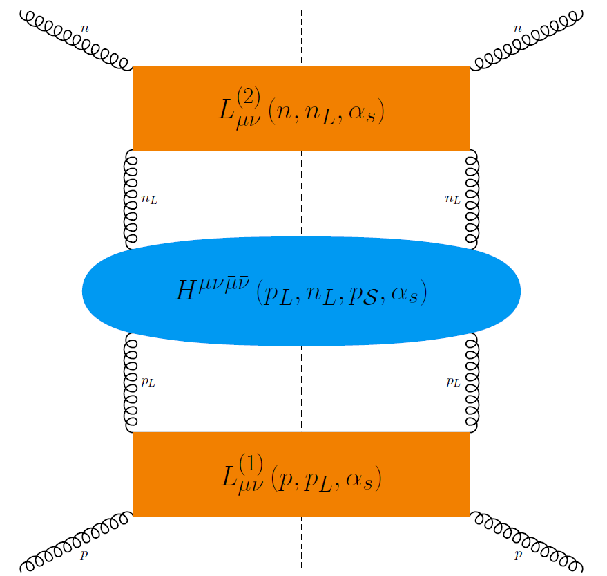
Figure 1: Factorization of the partonic cross section in a hard part and two ladder parts

The hard part and the ladders are both ultraviolet and collinear divergent; renormalization and factorization then introduces a dependence on the renormalization and factorization scales $\mu_{\rm\scriptscriptstyle\rm R}^{2}$ and $\mu_{\rm\scriptscriptstyle\rm F}^{2}$. Because the running of the coupling is logarithmically subleading (the coupling runs with the hard scale $Q^{2}$ and not with $s$), we can ignore the $\mu_{\rm\scriptscriptstyle\rm R}^{2}$ dependence, which only goes through $\alpha_{s}(\mu_{\rm\scriptscriptstyle\rm R}^{2})$ at the LL$x$ accuracy of our calculation. Furthermore, in order to simplify our derivation, we will assume that the hard part is two-particle irreducible, rather than just two-gluon irreducible, in which case it is free of collinear singularities Ellis:1978ty ; Curci:1980uw and it is thus independent of the factorization scale. The extension to the case in which the hard part is two-particle reducible and thus not collinear safe, such as deep-inelastic scattering Catani:1994sq or Drell-Yan production Marzani:2008uh is nontrivial, but it does not affect our argument, and it will not be considered here.

The most general structure of the hard part and the ladders compatible with Lorentz invariance and the Ward identities is then

$$H^{\mu\nu\bar{\mu}\bar{\nu}}\left(n_{L},p_{L},\Omega_{\mathcal{S}},\alpha_{s}\right)= \left(-g^{\mu\nu}+\frac{p_{L}^{\mu}p_{L}^{\nu}}{p_{L}^{2}}\right)\left(-g^{\bar{\mu}\bar{\nu}}+\frac{n_{L}^{\bar{\mu}}n_{L}^{\bar{\nu}}}{n_{L}^{2}}\right)H_{\perp,\perp}$$

$$+ \Bigg{[}n_{L}^{2}\left(-g^{\mu\nu}+\frac{p_{L}^{\mu}p_{L}^{\nu}}{p_{L}^{2}}\right)\left(\frac{n_{L}^{\bar{\mu}}}{n_{L}^{2}}-\frac{p_{L}^{\bar{\mu}}}{\left(n_{L}\cdot p_{L}\right)}\right)\left(\frac{n_{L}^{\bar{\nu}}}{n_{L}^{2}}-\frac{p_{L}^{\bar{\nu}}}{\left(n_{L}\cdot p_{L}\right)}\right)$$

$$+ p_{L}^{2}\left(\frac{p_{L}^{\mu}}{p_{L}^{2}}-\frac{n_{L}^{\mu}}{\left(n_{L}\cdot p_{L}\right)}\right)\left(\frac{p_{L}^{\nu}}{p_{L}^{2}}-\frac{n_{L}^{\nu}}{\left(n_{L}\cdot p_{L}\right)}\right)\left(-g^{\bar{\mu}\bar{\nu}}+\frac{n_{L}^{\bar{\mu}}n_{L}^{\bar{\nu}}}{n_{L}^{2}}\right)\Bigg{]}H_{\perp,\parallel}$$

$$+ p_{L}^{2}n_{L}^{2}\left(\frac{p_{L}^{\mu}}{p_{L}^{2}}-\frac{n_{L}^{\mu}}{\left(n_{L}\cdot p_{L}\right)}\right)\left(\frac{p_{L}^{\nu}}{p_{L}^{2}}-\frac{n_{L}^{\nu}}{\left(n_{L}\cdot p_{L}\right)}\right)$$

$$\left(\frac{n_{L}^{\bar{\mu}}}{n_{L}^{2}}-\frac{p_{L}^{\bar{\mu}}}{\left(n_{L}\cdot p_{L}\right)}\right)\left(\frac{n_{L}^{\bar{\nu}}}{n_{L}^{2}}-\frac{p_{L}^{\bar{\nu}}}{\left(n_{L}\cdot p_{L}\right)}\right)H_{\parallel,\parallel}$$

$$+ R^{\mu\nu\bar{\mu}\bar{\nu}}H_{\rm mixed}$$ (2.3a)

$$L^{\mu\nu}\left(p_{L},p,\mu_{\rm\scriptscriptstyle\rm F}^{2},\alpha_{s}\right)= \frac{1}{p_{L}^{2}}\left(-g^{\mu\nu}+\frac{p_{L}^{\mu}p_{L}^{\nu}}{p_{L}^{2}}\right)L^{(1)}_{\perp}$$

$$+ \left(\frac{p_{L}^{\mu}}{p_{L}^{2}}-\frac{p^{\mu}}{\left(p\cdot p_{L}\right)}\right)\left(\frac{p_{L}^{\nu}}{p_{L}^{2}}-\frac{p^{\nu}}{\left(p\cdot p_{L}\right)}\right)L^{(1)}_{\parallel}$$ (2.3b)

$$L^{\bar{\mu}\bar{\nu}}\left(n_{L},n,\mu_{\rm\scriptscriptstyle\rm F}^{2},\alpha_{s}\right)= \frac{1}{n_{L}^{2}}\left(-g^{\bar{\mu}\bar{\nu}}+\frac{n_{L}^{\bar{\mu}}n_{L}^{\bar{\nu}}}{n_{L}^{2}}\right)L^{(2)}_{\perp}$$

$$+ \left(\frac{n_{L}^{\bar{\mu}}}{n_{L}^{2}}-\frac{n^{\bar{\mu}}}{\left(n\cdot n_{L}\right)}\right)\left(\frac{n_{L}^{\bar{\nu}}}{n_{L}^{2}}-\frac{n^{\bar{\nu}}}{\left(n\cdot n_{L}\right)}\right)L^{(2)}_{\parallel},$$ (2.3c)

in terms of dimensionless scalar form factors

$$H_{\rm mixed}= H_{\rm mixed}\left(\frac{Q^{2}}{\left(n_{L}\cdot p_{L}\right)},\frac{-p_{L}^{2}}{Q^{2}},\frac{-n_{L}^{2}}{Q^{2}},\Omega_{\mathcal{S}},\alpha_{s}\right)$$ (2.4a)

$$H_{\{\perp,\parallel\},\{\perp,\parallel\}}= H_{\{\perp,\parallel\},\{\perp,\parallel\}}\left(\frac{Q^{2}}{\left(n_{L}\cdot p_{L}\right)},\frac{-p_{L}^{2}}{Q^{2}},\frac{-n_{L}^{2}}{Q^{2}},\Omega_{\mathcal{S}},\alpha_{s}\right)$$ (2.4b)

$$L^{(1)}_{\{\perp,\parallel\}}= L^{(1)}_{\{\perp,\parallel\}}\left(\frac{-p^{2}_{L}}{\left(p\cdot p_{L}\right)},\frac{\mu_{\rm\scriptscriptstyle\rm F}^{2}}{-p_{L}^{2}},\alpha_{s}\right)$$ (2.4c)

$$L^{(2)}_{\{\perp,\parallel\}}= L^{(2)}_{\{\perp,\parallel\}}\left(\frac{-n_{L}^{2}}{\left(n\cdot n_{L}\right)},\frac{\mu_{\rm\scriptscriptstyle\rm F}^{2}}{-n_{L}^{2}},\alpha_{s}\right),$$ (2.4d)

where with the notation $\{\perp,\parallel\}$ we mean that either of the two values can be chosen. The tensor $R^{\mu\nu\bar{\mu}\bar{\nu}}$ contains all terms which mix contribution coming from the two legs: it has a lengthy expression, but it turns out to only require a single further scalar form factor.

Equations (2.3) greatly simplify in the high energy limit. In order to study it, we define

$$x=\frac{Q^{2}}{s},$$ (2.5)

and we introduce a Sudakov parametrization for the two off-shell momenta $p_{L}$ and $n_{L}$:

$$p_{L}= z\,p-\mathbf{k}-\frac{k_{\rm\scriptscriptstyle\rm T}^{2}}{s\left(1-z\right)}\,n=\left(\sqrt{\frac{s}{2}}\,z,-\frac{k_{\rm\scriptscriptstyle\rm T}^{2}}{\sqrt{2s}\left(1-z\right)},-\mathbf{k}_{\scriptscriptstyle\rm T}\right)$$ (2.6a)

$$n_{L}= \bar{z}\,n-\mathbf{\bar{k}}-\frac{\bar{k}_{\scriptscriptstyle\rm T}^{2}}{s\left(1-\bar{z}\right)}\,p=\left(-\frac{\bar{k}_{\scriptscriptstyle\rm T}^{2}}{\sqrt{2s}\left(1-\bar{z}\right)},\sqrt{\frac{s}{2}}\,\bar{z},-\mathbf{\bar{k}}_{\scriptscriptstyle\rm T}\right),$$ (2.6b)

where $\mathbf{k}$ and $\mathbf{\bar{k}}$ are purely transverse spacelike four-vectors with $\mathbf{k}^{2}=-k_{\rm\scriptscriptstyle\rm T}^{2}<0$ and $\mathbf{\bar{k}}^{2}=-\bar{k}_{\scriptscriptstyle\rm T}^{2}<0$, and $s=2\left(p\cdot n\right)$. With this parametrization, the integration measures $\left[dp_{L}\right]$ and $\left[dn_{L}\right]$ are

$$\left[dp_{L}\right]=\frac{dz}{2\left(1-z\right)}d^{2}\mathbf{k};\qquad\left[dn_{L}\right]=\frac{d\bar{z}}{2\left(1-\bar{z}\right)}d^{2}\mathbf{\bar{k}}.$$ (2.7)

The high-energy limit is the limit in which $x\to 0$: we wish to determine the dominant power of $x$ contributing to $\sigma$, Eq. (2), with terms proportional to $\ln x$ included to all orders in $\alpha_{s}$ at the leading logarithmic (LL$x$) level. We then observe that, because the integration over $z$ and $\bar{z}$ ranges from $x$ to $1$, terms which are enhanced at small $x$ come from the small $z$ and $\bar{z}$ region. The moduli of the transverse momenta $k_{\rm\scriptscriptstyle\rm T}^{2}$ and $\bar{k_{\rm\scriptscriptstyle\rm T}^{2}}$ are of order of the hard scale $Q^{2}$ which bounds them from above, and thus in the high energy regime $Q^{2}\ll s$, they satisfy $\frac{k_{\rm\scriptscriptstyle\rm T}^{2}}{s}\ll 1$ and $\frac{\bar{k}_{\scriptscriptstyle\rm T}^{2}}{s}\ll 1$. Therefore, the high energy regime is

$$z\ll 1,\qquad\frac{k_{\rm\scriptscriptstyle\rm T}^{2}}{s}\ll 1;\qquad\qquad\bar{z}\ll 1,\qquad\frac{\bar{k}_{\scriptscriptstyle\rm T}^{2}}{s}\ll 1,$$ (2.8)

and subleading terms in $z$, $\bar{z}$, $\frac{k_{\rm\scriptscriptstyle\rm T}^{2}}{s}$ or $\frac{\bar{k}_{\scriptscriptstyle\rm T}^{2}}{s}$ upon integration lead to power-suppressed $\mathcal{O}\left(x\right)$ terms.

We can now simplify Eq. (2.3). First, we recall Ellis:1978ty that interference between emissions from different legs is power-suppressed in $s$. It follows that $H_{\rm mixed}$ Eq. (2.3a) is subleading. Furthermore, we note Caola:2010kv that in the limit Eq. (2.8) the dependence of the remaining scalar functions simplifies:

$$H_{\{\perp,\parallel\},\{\perp,\parallel\}}\left(\frac{Q^{2}}{\left(n_{L}\cdot p_{L}\right)},\frac{-p_{L}^{2}}{Q^{2}},\frac{-n_{L}^{2}}{Q^{2}},\Omega_{\mathcal{S}},\alpha_{s}\right)= H_{\{\perp,\parallel\},\{\perp,\parallel\}}\left(\frac{x}{z\bar{z}},\frac{k_{\rm\scriptscriptstyle\rm T}^{2}}{Q^{2}},\frac{\bar{k}_{\scriptscriptstyle\rm T}^{2}}{Q^{2}},\Omega_{\mathcal{S}},\alpha_{s}\right)\left(1+\mathcal{O}\left(z,\bar{z}\right)\right)$$ (2.9)

$$L^{(1)}_{\{\perp,\parallel\}}\left(\frac{-p^{2}_{L}}{\left(p\cdot p_{L}\right)},\frac{\mu_{\rm\scriptscriptstyle\rm F}^{2}}{-p_{L}^{2}},\alpha_{s}\right)= L^{(1)}_{\{\perp,\parallel\}}\left(\frac{\mu_{\rm\scriptscriptstyle\rm F}^{2}}{k_{\rm\scriptscriptstyle\rm T}^{2}},\alpha_{s}\right)\left(1+\mathcal{O}\left(z\right)\right)$$ (2.10)

$$L^{(2)}_{\{\perp,\parallel\}}\left(\frac{-n_{L}^{2}}{\left(n\cdot n_{L}\right)},\frac{\mu_{\rm\scriptscriptstyle\rm F}^{2}}{-n_{L}^{2}},\alpha_{s}\right)= L^{(2)}_{\{\perp,\parallel\}}\left(\frac{\mu_{\rm\scriptscriptstyle\rm F}^{2}}{\bar{k}_{\scriptscriptstyle\rm T}^{2}},\alpha_{s}\right)\left(1+\mathcal{O}\left(\bar{z}\right)\right)$$ (2.11)

up to terms that are suppressed by power of $z$ or $\bar{z}$. Finally, power counting arguments Ellis:1978ty ; Catani:1990eg lead to the conclusion that the transverse scalar functions Eq. (2.9) are no more singular that the longitudinal ones: it follows that the partonic cross section, Eq. (2) in the small $x$ limit has the form

$$\sigma\left(x,\frac{\mu^{2}_{F}}{Q^{2}}\right) =\int\left[\frac{x}{2z\bar{z}}H_{\parallel,\parallel}\left(\frac{x}{z\bar{z}},\frac{k_{\rm\scriptscriptstyle\rm T}^{2}}{Q^{2}},\frac{\bar{k}_{\scriptscriptstyle\rm T}^{2}}{Q^{2}},\Omega_{\mathcal{S}},\alpha_{s}\right)\right]$$

$$\;\left[2\pi L^{(1)}_{\parallel}\left(\frac{\mu_{\rm\scriptscriptstyle\rm F}^{2}}{k_{\rm\scriptscriptstyle\rm T}^{2}},\alpha_{s}\right)\right]\left[2\pi L^{(2)}_{\parallel}\left(\frac{\mu_{\rm\scriptscriptstyle\rm F}^{2}}{\bar{k}_{\scriptscriptstyle\rm T}^{2}},\alpha_{s}\right)\right]\frac{dz}{z}\frac{d\bar{z}}{\bar{z}}\frac{dk_{\rm\scriptscriptstyle\rm T}^{2}}{k_{\rm\scriptscriptstyle\rm T}^{2}}\frac{d\bar{k}_{\scriptscriptstyle\rm T}^{2}}{\bar{k}_{\scriptscriptstyle\rm T}^{2}}\frac{d\theta}{2\pi}\frac{d\bar{\theta}}{2\pi}+\mathcal{O}\left(z,\bar{z}\right),$$ (2.12)

where $\theta$ and $\bar{\theta}$ are the azimuthal angles of the transverse momenta $\mathbf{k}$ and $\mathbf{\bar{k}}$, and at LL$x$ $\alpha_{s}$ is fixed, and thus $\sigma$ is $\mu_{R}$-independent.

We note that the dependence on $\theta$ and $\bar{\theta}$ is entirely contained in the hard part. Also, in the high-energy limit the longitudinal projectors which carry the tensor structure of the term proportional to $H_{\parallel,\parallel}$ Eq. (2.3) reduce to Catani:1990eg

$$\mathcal{P}^{\mu\nu}=\frac{k^{\mu}k^{\nu}}{k_{\rm\scriptscriptstyle\rm T}^{2}};\qquad\mathcal{P}^{\bar{\mu}\bar{\nu}}=\frac{\bar{k}^{\bar{\mu}}\bar{k}^{\bar{\nu}}}{\bar{k}_{\scriptscriptstyle\rm T}^{2}}.$$ (2.13)

We can thus rewrite the cross-section Eq. (2) in terms of a generalized coefficient function

$$C\left(\frac{x}{z\bar{z}},\frac{k_{\rm\scriptscriptstyle\rm T}^{2}}{Q^{2}},\frac{\bar{k}_{\scriptscriptstyle\rm T}^{2}}{Q^{2}},\alpha_{s}\right) \equiv\int\frac{d\theta}{2\pi}\frac{d\bar{\theta}}{2\pi}\,\frac{x}{2z\bar{z}}H_{\parallel,\parallel}\left(\frac{x}{z\bar{z}},\frac{k_{\rm\scriptscriptstyle\rm T}^{2}}{Q^{2}},\frac{\bar{k}_{\scriptscriptstyle\rm T}^{2}}{Q^{2}},\Omega_{\mathcal{S}},\alpha_{s}\right)$$

$$=\int\frac{d\theta}{2\pi}\frac{d\bar{\theta}}{2\pi}\,\frac{x}{2z\bar{z}}\left[\mathcal{P}^{\mu\nu}\mathcal{P}^{\bar{\mu}\bar{\nu}}H_{\mu\nu\bar{\mu}\bar{\nu}}\right].$$ (2.14)

The coefficient function Eq. (2.14) is recognized as the cross section for the partonic process

$$g^{*}\left(q\right)+g^{*}\left(r\right)\to\mathcal{S}$$ (2.15)

with two incoming off-shell gluon with momenta

$$q=zp+k\qquad q^{2}=-k_{\rm\scriptscriptstyle\rm T}^{2}$$ (2.16)

$$r=\bar{z}n+\bar{k}\qquad r^{2}=-\bar{k}_{\scriptscriptstyle\rm T}^{2},$$ (2.17)

and the projectors Eq. (2.13) viewed as polarization sums.

Because the hard part is 2GI, the coefficient function is regular in the $x\to 0$ limit, and small $x$ singularities are only contained in the ladders. In Ref. Catani:1990xk ; Catani:1990eg they are computed at LL$x$ level in terms of a gluon Green function, which in turns sum leading logs of $x$ by iterating a BFKL Lipatov:polo kernel. In Ref. Caola:2010kv they were instead determined using the generalized ladder expansion of Ref. Curci:1980uw . This derivation is closer to that of standard collinear factorization, and thus more suitable to applications of high-energy resummation to standard, collinear-factorized hard partonic cross-section, and specifically to its extension to less inclusive quantities.

The ladders contain collinear singularities that must be factorized in the parton distributions after regularization; this can be done in an iterative way Curci:1980uw which also leads to small $x$ resummation, as explained in Ref. Caola:2010kv , which we follow in view of our desired generalization. In this approach, the ladders $L^{(1)}_{\parallel}$ and $L^{(2)}_{\parallel}$ are obtained by iteration of a 2GI kernel $K\left(p_{i},p_{i-1},\mu,\alpha_{s}\right)$ or $K\left(n_{i},n_{i-1},\mu,\alpha_{s}\right)$ with $i=1,2,\dots,n$, connected by a pair of $t$-channel gluons (see Fig. 2). The transverse momenta of the gluons are ordered, ${k_{\rm\scriptscriptstyle\rm T}^{2}}\,_{1}\ll{k_{\rm\scriptscriptstyle\rm T}^{2}}\,_{2}\ll\dots\ll{k_{\rm\scriptscriptstyle\rm T}^{2}}\,_{n}=k_{\rm\scriptscriptstyle\rm T}^{2}$ (and ${\bar{k}_{\scriptscriptstyle\rm T}^{2}}\,_{1}\ll{\bar{k}_{\scriptscriptstyle\rm T}^{2}}\,_{2}\ll\dots\ll{\bar{k}_{\scriptscriptstyle\rm T}^{2}}\,_{n}=\bar{k}_{\scriptscriptstyle\rm T}^{2}$), with small $x$ resummation performed by computing the kernels at LL$x$ to all orders in $\alpha_{s}$.

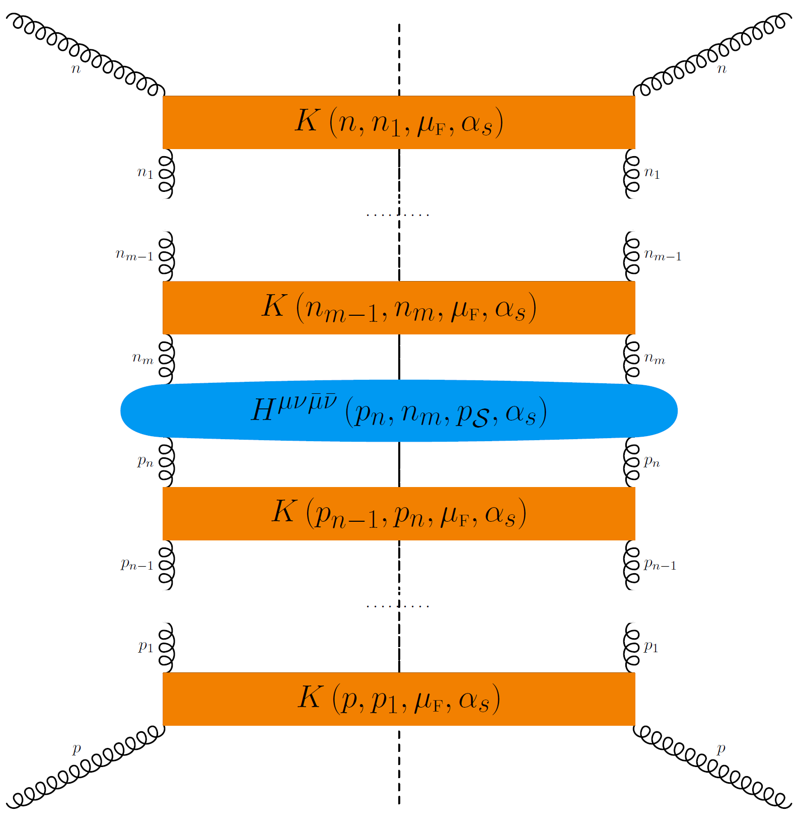
Figure 2: Computation of the ladder parts by iterative insertion of the Kernel $K$

We start from a regularized version of the expression Eq. (2) for the cross-section, written in terms of the coefficient function $C$, Eq. (2.14):

$$\sigma\left(x,\frac{\mu_{\rm\scriptscriptstyle\rm F}^{2}}{Q^{2}},\alpha_{s};\epsilon\right)=\left(Q^{2}\right)^{2\epsilon}\int C\left(\frac{x}{z\bar{z}},\frac{k_{\rm\scriptscriptstyle\rm T}^{2}}{Q^{2}},\frac{\bar{k}_{\scriptscriptstyle\rm T}^{2}}{Q^{2}},\alpha_{s};\epsilon\right)\left[2\pi L^{(1)}_{\parallel}\left(z,\left(\frac{\mu_{\rm\scriptscriptstyle\rm F}^{2}}{k_{\rm\scriptscriptstyle\rm T}^{2}}\right)^{\epsilon},\alpha_{s};\epsilon\right)\right]$$

$$\left[2\pi L^{(2)}_{\parallel}\left(\bar{z},\left(\frac{\mu_{\rm\scriptscriptstyle\rm F}^{2}}{\bar{k}_{\scriptscriptstyle\rm T}^{2}}\right)^{\epsilon},\alpha_{s};\epsilon\right)\right]\frac{dz}{z}\frac{d\bar{z}}{\bar{z}}\frac{dk_{\rm\scriptscriptstyle\rm T}^{2}}{\left(k_{\rm\scriptscriptstyle\rm T}^{2}\right)^{1+\epsilon}}\frac{d\bar{k}_{\scriptscriptstyle\rm T}^{2}}{\left(\bar{k}_{\scriptscriptstyle\rm T}^{2}\right)^{1+\epsilon}},$$ (2.18)

where the dependence on $z$ and $\bar{z}$ in the ladders is $\mathcal{O}(\epsilon)$ Caola:2010kv . We factorize, as usual, the convolutions by Mellin transformation

$$\sigma\left(N,\frac{\mu_{\rm\scriptscriptstyle\rm F}^{2}}{Q^{2}},\alpha_{s};\epsilon\right)= \int_{0}^{\infty}\frac{d\xi}{\xi^{1+\epsilon}}\int_{0}^{\infty}\frac{d\bar{\xi}}{\bar{\xi}^{1+\epsilon}}C\left(N,\xi,\bar{\xi},\alpha_{s};\epsilon\right)$$

$$\left[2\pi L^{(1)}_{\parallel}\left(N,\left(\frac{\mu_{\rm\scriptscriptstyle\rm F}^{2}}{Q^{2}\xi}\right)^{\epsilon},\alpha_{s};\epsilon\right)\right]\left[2\pi L^{(2)}_{\parallel}\left(N,\left(\frac{\mu_{\rm\scriptscriptstyle\rm F}^{2}}{Q^{2}\bar{\xi}}\right)^{\epsilon},\alpha_{s};\epsilon\right)\right],$$ (2.19)

with

$$f(N)=\int_{0}^{1}dx\,x^{N-1}f(x);\qquad f(x)= \frac{1}{2\pi i}\int_{N_{0}-i\infty}^{N_{0}+i\infty}dN\,x^{-N}f(N),$$ (2.20)

where we have introduced dimensionless variables

$$\xi=\frac{k_{\rm\scriptscriptstyle\rm T}^{2}}{Q^{2}},\qquad\bar{\xi}=\frac{\bar{k}_{\scriptscriptstyle\rm T}^{2}}{Q^{2}}.$$ (2.21)

Note that the $Q^{2}$-dependence of the ladders is fictitious, as $\frac{\mu_{\rm\scriptscriptstyle\rm F}^{2}}{Q^{2}\xi}=\frac{\mu_{\rm\scriptscriptstyle\rm F}^{2}}{k_{\rm\scriptscriptstyle\rm T}^{2}}$. Upon Mellin transformation, powers of $\ln\frac{1}{x}$ are mapped onto poles at $N=0$: note that the Mellin variable in Eq. (2.20), as usual in the context of high-energy resummation, is shifted by one unit in comparison to the more customary definition.

The observation Curci:1980uw that collinear poles in $\epsilon$ are all produced by the integrations over the transverse momenta ${k_{\rm\scriptscriptstyle\rm T}^{2}}$, $\bar{k}_{\scriptscriptstyle\rm T}^{2}$ connecting the kernels leads to the identification of the kernel itself with the anomalous dimension $\gamma$ in $d=4-2\epsilon$ dimensions, which in our case must be computed to all orders in $\alpha_{s}$ to LL$x$ accuracy Caola:2010kv :

$$K\left(N,\left(\frac{\mu_{\rm\scriptscriptstyle\rm F}^{2}}{Q^{2}{\xi}}\right)^{\epsilon},\alpha_{s};\epsilon\right)=\gamma\left(N,\left(\frac{\mu_{\rm\scriptscriptstyle\rm F}^{2}}{Q^{2}\xi}\right)^{\epsilon},\alpha_{s};\epsilon\right).$$ (2.22)

The ladder expansion of $L^{(1,2)}$ at LL$x$ then has the form

$$\sigma^{n,m}\left(N,\frac{\mu_{\rm\scriptscriptstyle\rm F}^{2}}{Q^{2}},\alpha_{s};\epsilon\right)=\int_{0}^{\infty}\left[\gamma\left(N,\left(\frac{\mu_{\rm\scriptscriptstyle\rm F}^{2}}{Q^{2}\xi_{n}}\right)^{\epsilon},\alpha_{s};\epsilon\right)\right]\frac{d\xi_{n}}{\xi_{n}^{1+\epsilon}}\times$$

$$\times\int_{0}^{\infty}\left[\gamma\left(N,\left(\frac{\mu_{\rm\scriptscriptstyle\rm F}^{2}}{Q^{2}\bar{\xi}_{m}}\right)^{\epsilon},\alpha_{s};\epsilon\right)\right]\frac{d\bar{\xi}_{m}}{\bar{\xi}_{m}^{1+\epsilon}}C\left(N,\xi,\bar{\xi},\alpha_{s};\epsilon\right)\times$$ (2.23)

$$\times\int_{0}^{\xi_{n}}\left[\gamma\left(N,\left(\frac{\mu_{\rm\scriptscriptstyle\rm F}^{2}}{Q^{2}\xi_{n-1}}\right)^{\epsilon},\alpha_{s};\epsilon\right)\right]\frac{d\xi_{n-1}}{\xi_{n-1}^{1+\epsilon}}\times\dots\times\int_{0}^{\xi_{2}}\left[\gamma\left(N,\left(\frac{\mu_{\rm\scriptscriptstyle\rm F}^{2}}{Q^{2}\xi_{1}}\right)^{\epsilon},\alpha_{s};\epsilon\right)\right]\frac{d\xi_{1}}{\xi_{1}^{1+\epsilon}}\times$$

$$\times\int_{0}^{\bar{\xi}_{m}}\left[\gamma\left(N,\left(\frac{\mu_{\rm\scriptscriptstyle\rm F}^{2}}{Q^{2}\bar{\xi}_{m-1}}\right)^{\epsilon},\alpha_{s};\epsilon\right)\right]\frac{d\bar{\xi}_{m-1}}{\bar{\xi}_{m-1}^{1+\epsilon}}\times\dots\times\int_{0}^{\bar{\xi}_{2}}\left[\gamma\left(N,\left(\frac{\mu_{\rm\scriptscriptstyle\rm F}^{2}}{Q^{2}\bar{\xi}_{1}}\right)^{\epsilon},\alpha_{s};\epsilon\right)\right]\frac{d\bar{\xi}_{1}}{\bar{\xi}_{1}^{1+\epsilon}}.$$

Factorization is performed by requiring Eq. (2) to be finite after each $\xi_{i}$ or $\bar{\xi}_{j}$ integration. This leave a single $n+m$-th order $\epsilon$ pole in the cross-section that can be subtracted using the standard $\overline{\rm MS}$ prescription (see Appendix A of Ref. Caola:2010kv ). After iterative subtraction of the first $n-1$ and $m-1$ singularities we get

$$\sigma^{n,m}\left(N,\frac{\mu_{\rm\scriptscriptstyle\rm F}^{2}}{Q^{2}},\alpha_{s};\epsilon\right)=\left[\gamma\left(N,\left(\frac{\mu_{\rm\scriptscriptstyle\rm F}^{2}}{Q^{2}}\right)^{\epsilon},\alpha_{s};\epsilon\right)\right]^{2}\int_{0}^{\infty}\frac{d\xi_{n}}{\xi_{n}^{1+\epsilon}}\int_{0}^{\infty}\frac{d\bar{\xi}_{m}}{\bar{\xi}_{m}^{1+\epsilon}}C\left(N,\xi_{n},\bar{\xi}_{m},\alpha_{s};\epsilon\right)\times$$

$$\times\frac{1}{\left(n-1\right)!}\frac{1}{\epsilon^{n-1}}\left[\sum_{j}\frac{\tilde{\gamma}_{j}\left(N,\alpha_{s};0\right)}{j}\left(1-\left(\frac{\mu_{\rm\scriptscriptstyle\rm F}^{2}}{Q^{2}\xi_{n}}\right)^{j\epsilon}\frac{\tilde{\gamma}_{i}\left(N,\alpha_{s};\epsilon\right)}{\tilde{\gamma}_{i}\left(N,\alpha_{s};0\right)}\right)\right]^{n-1}\times$$ (2.24)

$$\times\frac{1}{\left(m-1\right)!}\frac{1}{\epsilon^{m-1}}\left[\sum_{l}\frac{\tilde{\gamma}_{l}\left(N,\alpha_{s};0\right)}{l}\left(1-\left(\frac{\mu_{\rm\scriptscriptstyle\rm F}^{2}}{Q^{2}\bar{\xi}_{m}}\right)^{l\epsilon}\frac{\tilde{\gamma}_{i}\left(N,\alpha_{s};\epsilon\right)}{\tilde{\gamma}_{l}\left(N,\alpha_{s};0\right)}\right)\right]^{m-1}.$$

where we have introduced the expansion

$$\gamma\left(N,\left(\frac{\mu_{\rm\scriptscriptstyle\rm F}^{2}}{Q^{2}\xi}\right)^{\epsilon},\alpha_{s};\epsilon\right)=\sum_{j=0}^{\infty}\tilde{\gamma}_{j}\left(N,\alpha_{s};\epsilon\right)\left(\frac{\mu_{\rm\scriptscriptstyle\rm F}^{2}}{Q^{2}\xi}\right)^{j\epsilon}.$$ (2.25)

Summing over $n$ and $m$ the collinear singularities exponentiate:

$$\sigma_{\rm res} =\sum_{n,m=0}^{\infty}\sigma^{n,m}=\gamma\left(N,\left(\frac{\mu_{\rm\scriptscriptstyle\rm F}^{2}}{Q^{2}}\right)^{\epsilon},\alpha_{s};\epsilon\right)^{2}\int_{0}^{\infty}\frac{d\xi}{\xi^{1+\epsilon}}\int_{0}^{\infty}\frac{d\bar{\xi}}{\bar{\xi}^{1+\epsilon}}\,C\left(N,\xi,\bar{\xi},\alpha_{s};\epsilon\right)\times$$

$$\times\exp\left[\frac{1}{\epsilon}\sum_{j}\frac{\tilde{\gamma}_{j}\left(N,\alpha_{s};0\right)}{j}\left(1-\left(\frac{\mu_{\rm\scriptscriptstyle\rm F}^{2}}{Q^{2}\xi}\right)^{j\epsilon}\frac{\tilde{\gamma}_{j}\left(N,\alpha_{s};\epsilon\right)}{\tilde{\gamma}_{j}\left(N,\alpha_{s};0\right)}\right)\right]\times$$ (2.26)

$$\times\exp\left[\frac{1}{\epsilon}\sum_{l}\frac{\tilde{\gamma}_{l}\left(N,\alpha_{s};0\right)}{l}\left(1-\left(\frac{\mu_{\rm\scriptscriptstyle\rm F}^{2}}{Q^{2}\bar{\xi}}\right)^{l\epsilon}\frac{\tilde{\gamma}_{l}\left(N,\alpha_{s};\epsilon\right)}{\tilde{\gamma}_{l}\left(N,\alpha_{s};0\right)}\right)\right].$$

The limit $\epsilon\to 0$ can then be taken after expanding

$$\tilde{\gamma}_{i}\equiv\tilde{\gamma}_{i}\left(N,\alpha_{s}\right)+\epsilon\dot{\tilde{\gamma}}_{i}\left(N,\alpha_{s}\right)+\epsilon^{2}\ddot{\tilde{\gamma}}_{i}\left(N,\alpha_{s}\right)+\dots,$$ (2.27)

with the result

$$\sigma_{\rm res}\left(N,\alpha_{s}\right)=\gamma\left(N,\alpha_{s}\right)^{2}\mathcal{R}\left(N,\alpha_{s}\right)^{2} \int_{0}^{\infty}d\xi\,\xi^{\gamma\left(N,\alpha_{s}\right)-1}\int_{0}^{\infty}d\bar{\xi}\,\bar{\xi}^{\gamma\left(N,\alpha_{s}\right)-1}\,C\left(N,\xi,\bar{\xi},\alpha_{s}\right)$$

$$\times\exp\left[2\gamma\left(N,\alpha_{s}\right)\ln\frac{Q^{2}}{\mu_{\rm\scriptscriptstyle\rm F}^{2}}\right]$$ (2.28)

with Caola:2010kv

$$\mathcal{R}\left(N,\alpha_{s}\right)\equiv\exp\left[-\sum_{i}\frac{\dot{\tilde{\gamma}}_{i}\left(N,\alpha_{s}\right)}{i}\right].$$ (2.29)

Equation (2) is the resummed form of the partonic cross section at LL$x$ in the $\overline{\rm MS}$ scheme, after factorization of all singularities. The factor $\mathcal{R}$ depends on the choice of factorization scheme Caola:2010kv ; Catani:1990eg ; further scheme changes may be performed by redefining the parton distribution of the gluon by a generic LL$x$ function $\mathcal{N}\left(N,\alpha_{s}\right)$ Ball:1995np , after which all the scheme dependence can be collected in a prefactor

$$R\left(N,\alpha_{s}\right)=\mathcal{R}\left(N,\alpha_{s}\right)\mathcal{N}\left(N,\alpha_{s}\right).$$ (2.30)

Choosing $\mu_{\rm\scriptscriptstyle\rm F}^{2}=Q^{2}$ the final form of the resummed inclusive cross section is

$$\sigma_{\rm res}\left(N,\alpha_{s}\right)=\gamma\left(\frac{\alpha_{s}}{N}\right)^{2}R\left(\frac{\alpha_{s}}{N}\right)^{2}\int_{0}^{\infty}d\xi\,\xi^{\gamma\left(\frac{\alpha_{s}}{N}\right)-1}\int_{0}^{\infty}d\bar{\xi}\,\bar{\xi}^{\gamma\left(\frac{\alpha_{s}}{N}\right)-1}\,C\left(N,\xi,\bar{\xi},\alpha_{s}\right).$$ (2.31)

where we have explicitly indicated that, at LL$x$, $\gamma$ and $R$ only depend on the ratio $\alpha_{s}/N$.

In order to make contact with the approach of Ref. Catani:1990eg , it is useful to rewrite the resummed cross-section in terms of the so-called impact factor, defined as

$$h\left(N,M_{1},M_{2},\alpha_{s}\right)=M_{1}M_{2}\,R\left(M_{1}\right)R\left(M_{2}\right)\int_{0}^{\infty}d\xi\,\xi^{M_{1}-1}\int_{0}^{\infty}d\bar{\xi}\,\bar{\xi}^{M_{2}-1}\,C\left(N,\xi,\bar{\xi},\alpha_{s}\right),$$ (2.32)

in terms of which the cross-section Eq. (2.31) has the form

$$\sigma_{\rm res}\left(N,\alpha_{s}\right)=h\left(N,\gamma\left(\frac{\alpha_{s}}{N}\right),\gamma\left(\frac{\alpha_{s}}{N}\right),\alpha_{s}\right).$$ (2.33)

The explicit expressions of the LL$x$ anomalous dimension $\gamma$ and the factorization-scheme dependent function $R$ can be found e.g. in Ref. Catani:1994sq .

3 The transverse momentum distribution

Having briefly reviewed the approach of Ref. Caola:2010kv to high-energy resummation, we now extend it to transverse momentum distributions: the generalization turns out to be in fact completely straightforward, once the kinematics is properly understood.

We consider again the process Eq. (2.1), but now assuming that $\mathcal{S}$ has fixed transverse momentum $p_{\rm\scriptscriptstyle\rm T}$. Clearly (see Fig. 1) $p_{\rm\scriptscriptstyle\rm T}$ is the sum of the transverse momenta $k_{\rm\scriptscriptstyle\rm T}$ and $\bar{k}_{\scriptscriptstyle\rm T}$, of the gluons which connect the hard part to the ladder, so in the high-energy limit Eq. (2.8) it must satisfy

$$\frac{p_{\rm\scriptscriptstyle\rm T}^{2}}{s}\ll 1.$$ (3.1)

The factorization Eq. (2), which was derived by power counting from the conditions Eq. (2.8) still holds, but now with a kinematic constraint relating $p_{\rm\scriptscriptstyle\rm T}$ to $k_{\rm\scriptscriptstyle\rm T}$ and $\bar{k}_{\scriptscriptstyle\rm T}$:

$$\frac{d\sigma}{dp_{\rm\scriptscriptstyle\rm T}^{2}}=Q^{2}\,\int \left[\frac{x}{2z\bar{z}}H_{\parallel,\parallel}\left(\frac{x}{z\bar{z}},\frac{k_{\rm\scriptscriptstyle\rm T}^{2}}{Q^{2}},\frac{\bar{k}_{\scriptscriptstyle\rm T}^{2}}{Q^{2}},\Omega_{\mathcal{S}},\alpha_{s}\right)\right]\delta\left(p_{\rm\scriptscriptstyle\rm T}^{2}-k_{\rm\scriptscriptstyle\rm T}^{2}-\bar{k}_{\scriptscriptstyle\rm T}^{2}-2\sqrt{k_{\rm\scriptscriptstyle\rm T}^{2}\bar{k}_{\scriptscriptstyle\rm T}^{2}}\cos\theta\right)$$

$$\left[2\pi L^{(1)}_{\parallel}\left(\frac{\mu_{\rm\scriptscriptstyle\rm F}^{2}}{k_{\rm\scriptscriptstyle\rm T}^{2}},\alpha_{s}\right)\right]\left[2\pi L^{(2)}_{\parallel}\left(\frac{\mu_{\rm\scriptscriptstyle\rm F}^{2}}{\bar{k}_{\scriptscriptstyle\rm T}^{2}},\alpha_{s}\right)\right]\frac{dz}{z}\frac{d\bar{z}}{\bar{z}}\frac{dk_{\rm\scriptscriptstyle\rm T}^{2}}{k_{\rm\scriptscriptstyle\rm T}^{2}}\frac{d\bar{k}_{\scriptscriptstyle\rm T}^{2}}{\bar{k}_{\scriptscriptstyle\rm T}^{2}}\frac{d\theta}{2\pi}\frac{d\bar{\theta}}{2\pi}.$$ (3.2)

The constraint is a simple momentum conservation delta as a consequence of the fact that radiation is entirely contained in the ladders, and it does not take place from the hard part; without loss of generality, we have chosen $\theta$ as the angle between the directions of $\mathbf{k}$ and $\mathbf{\bar{k}}$.

We then define a $p_{\rm\scriptscriptstyle\rm T}$-dependent coefficient function

$$C_{p_{\rm\scriptscriptstyle\rm T}}\left(\frac{x}{z\bar{z}},\xi,\bar{\xi},\xi_{p},\alpha_{s}\right)=$$

$$\qquad=\int\frac{d\theta}{2\pi}\frac{d\bar{\theta}}{2\pi}\,\frac{x}{2z\bar{z}}H_{\parallel,\parallel}\left(\frac{x}{z\bar{z}},\xi,\bar{\xi},\Omega_{\mathcal{S}},\alpha_{s}\right)\delta\left(\xi_{p}-\xi-\bar{\xi}-2\sqrt{\xi\bar{\xi}}\cos\theta\right)$$

$$\qquad=\int\frac{d\theta}{2\pi}\frac{d\bar{\theta}}{2\pi}\,\frac{x}{2z\bar{z}}\left[\mathcal{P}^{\mu\nu}\mathcal{P}^{\bar{\mu}\bar{\nu}}H_{\mu\nu\bar{\mu}\bar{\nu}}\right]\delta\left(\xi_{p}-\xi-\bar{\xi}-2\sqrt{\xi\bar{\xi}}\cos\theta\right)$$ (3.3)

where we have introduced a further dimensionless variable

$$\xi_{p}=\frac{p_{\rm\scriptscriptstyle\rm T}^{2}}{Q^{2}},$$ (3.4)

on top of $\xi$, $\bar{\xi}$ Eq. (2.21). In terms of $C_{p_{\rm\scriptscriptstyle\rm T}}$, Eq. (3) becomes

$$\frac{d\sigma}{d\xi_{p}}=\int C_{p_{\rm\scriptscriptstyle\rm T}}\left(\frac{x}{z\bar{z}},\xi,\bar{\xi},\bar{\xi_{p}},\alpha_{s}\right)$$

$$\times\left[2\pi L^{(1)}_{\parallel}\left(\frac{\mu_{\rm\scriptscriptstyle\rm F}^{2}}{Q^{2}\xi},\alpha_{s}\right)\right]\left[2\pi L^{(2)}_{\parallel}\left(\frac{\mu_{\rm\scriptscriptstyle\rm F}^{2}}{Q^{2}\bar{\xi}},\alpha_{s}\right)\right]\frac{dz}{z}\frac{d\bar{z}}{\bar{z}}\frac{d\xi}{\xi}\frac{d\bar{\xi}}{\bar{\xi}}.$$ (3.5)

The coefficient function $C_{p_{\rm\scriptscriptstyle\rm T}}$ is the transverse momentum distribution for the production of $\mathcal{S}$ from two off-shell gluons with transverse momenta $\mathbf{k}$ and $\mathbf{\bar{k}}$.

We now turn to the ladders. Each insertion of the LL$x$ kernel $K$ Eq. (2.22) includes an infinite series of $s$- and $t$-channel branchings Ball:1997vf , which can be viewed as a single effective emission vertex. The momenta of the gluons $q_{1}$,…,$q_{L}$ and $r_{1}$,…,$r_{L}$ respectively radiated from each of the two rails of the ladder, and of the gluons $p_{1}$,…,$p_{L}$ and $n_{1}$,…,$n_{L}$ respectively propagating along them, in the Sudakov parametrization in the high-energy limit can be written as (see Fig. 3)

$$p_{1} =z_{1}p-\mathbf{k}_{1}$$ (3.6a)

$$q_{1} =\left(1-z_{1}\right)p+\mathbf{k}_{1}$$ (3.6b)

$$p_{2} =z_{2}z_{1}p-\mathbf{k}_{2}$$ (3.6c)

$$q_{2} =\left(1-z_{1}z_{2}\right)z_{1}p+\mathbf{k}_{2}-\mathbf{k}_{1}$$ (3.6d)

$$\dots\dots\dots$$ (3.6e)

$$p_{L} =zp-\mathbf{k}$$ (3.6f)

$$q_{L} =\left(1-z\right)p+\mathbf{k}-\mathbf{k_{n-1}}$$ (3.6g)

$$n_{1} =\bar{z}_{1}p-\mathbf{\bar{k}}_{1}$$ (3.6h)

$$r_{1} =\left(1-\bar{z}_{1}\right)p+\mathbf{\bar{k}}_{1}$$ (3.6i)

$$n_{2} =\bar{z}_{2}\bar{z}_{1}p-\mathbf{\bar{k}}_{2}$$ (3.6j)

$$r_{2} =\left(1-\bar{z}_{1}\bar{z}_{2}\right)\bar{z}_{1}p+\mathbf{\bar{k}}_{2}-\mathbf{\bar{k}}_{1}$$ (3.6k)

$$\dots\dots\dots$$ (3.6l)

$$n_{L} =\bar{z}n-\mathbf{\bar{k}}$$ (3.6m)

$$r_{L} =\left(1-\bar{z}\right)n+\mathbf{\bar{k}-\mathbf{\bar{k}_{m-1}}}.$$ (3.6n)

The crucial observation here is that the momenta of the emitted gluons $q_{1}$ and $r_{i}$ are integrated over. So, for instance, the transverse momentum of the second emitted gluon is an integration variable, and we can equivalently choose it as $\mathbf{k}_{2}$ or, shifting the integration variable, as $\mathbf{k}_{2}-\mathbf{k}_{1}$, as in Eq. (3.6d). With the choice of integration variables of Eq. (3.6), it is manifest that all the transverse momenta $\mathbf{k}_{i}$ and $\mathbf{\bar{k}}_{j}$ are independent, with the only ordering constraints $k_{\scriptscriptstyle\rm T,1}^{2}\ll k_{\scriptscriptstyle\rm T,2}^{2}\ll\dots\ll k_{\scriptscriptstyle\rm T}^{2}$ and $\bar{k}_{\scriptscriptstyle\rm T,1}^{2}\ll\bar{k}_{\scriptscriptstyle\rm T,2}^{2}\ll\dots\ll\bar{k}_{\scriptscriptstyle\rm T}^{2}$. The fixed value of $p_{\rm\scriptscriptstyle\rm T}^{2}$ of the final state $\mathcal{S}$ thus only constrains the transverse components of the momenta $p_{L}$ $n_{L}$ of the two gluons entering the hard part $H$. The dependence on the longitudinal momentum fractions in Eq. (3.6) is immaterial for our purposes, and was discussed in Ref. Caola:2010kv .

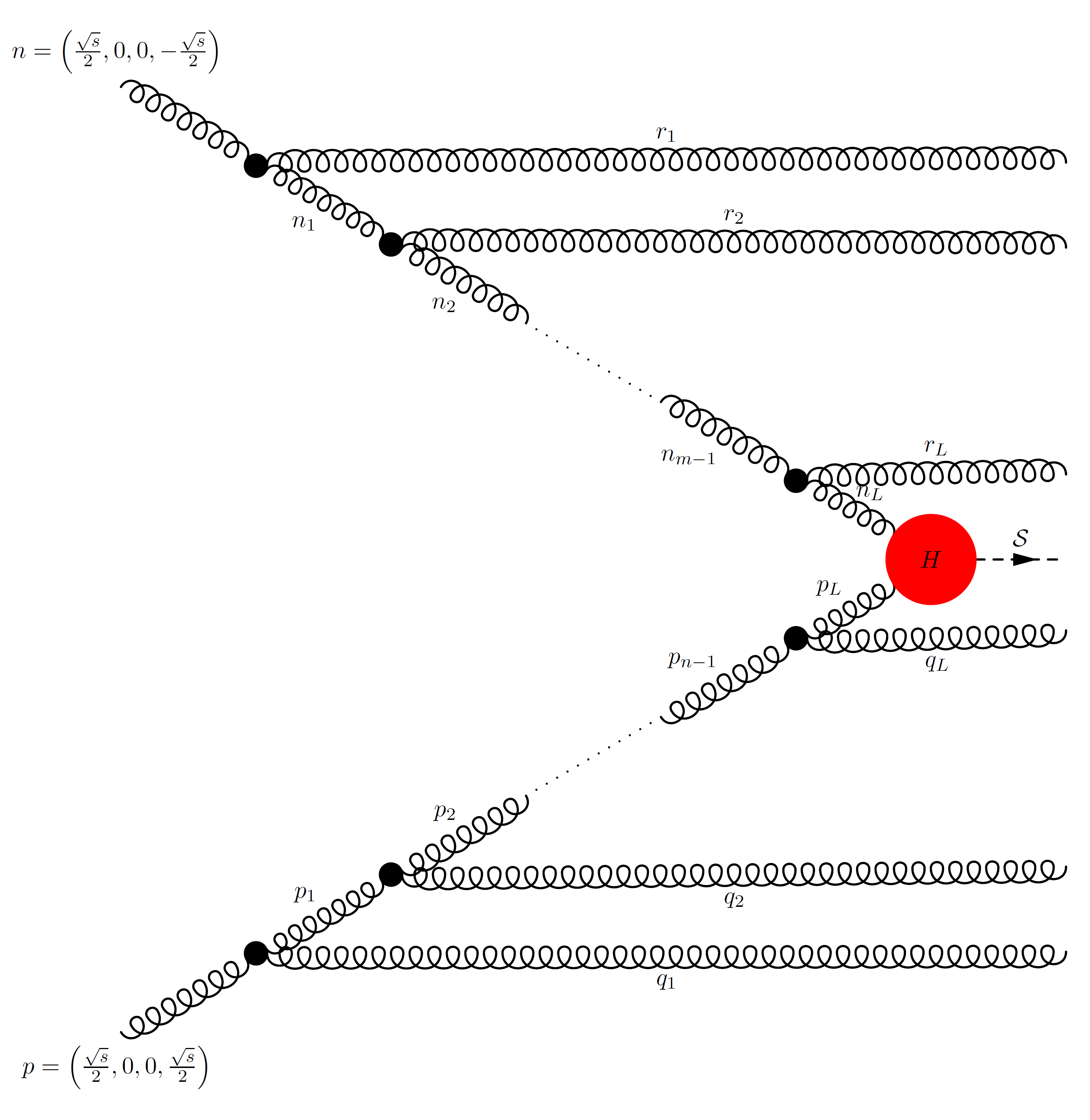
Figure 3: Kinematics of the ladder. The blob at each emission vertex denotes inclusion of LL$x$ $s$- and $t$-channel gluon radiation to all orders.

It follows that we can compute the ladders as in the inclusive case, the only difference being in the integration over the transverse momenta of the two gluons connecting each ladder to the hard part: we iterate the kernel $K$ and sum over all possible insertions. The regularized contribution to the transverse momentum distribution when the kernel $K$ is inserted $n$-th times on one leg and $m$-th times on the other leg, after the iterative subtraction of the first $n-1$ and $m-1$ collinear singularities has the form

$$\frac{d\sigma^{n,m}}{d\xi_{p}}\left(N,\frac{\mu_{\rm\scriptscriptstyle\rm F}^{2}}{Q^{2}},\xi_{p},\alpha_{s};\epsilon\right)=\left[\gamma\left(N,\left(\frac{\mu_{\rm\scriptscriptstyle\rm F}^{2}}{Q^{2}}\right)^{\epsilon},\alpha_{s};\epsilon\right)\right]^{2}$$

$$\times\int_{0}^{\infty}\frac{d\xi_{n}}{\xi_{n}^{1+\epsilon}}\int_{0}^{\infty}\frac{d\bar{\xi}_{m}}{\bar{\xi}_{m}^{1+\epsilon}}C_{p_{\rm\scriptscriptstyle\rm T}}\left(N,\xi_{n},\bar{\xi}_{m},\xi_{p},\alpha_{s};\epsilon\right)\times$$

$$\times\frac{1}{\left(n-1\right)!}\frac{1}{\epsilon^{n-1}}\left[\sum_{j}\frac{\tilde{\gamma}_{j}\left(N,\alpha_{s};0\right)}{j}\left(1-\left(\frac{\mu_{\rm\scriptscriptstyle\rm F}^{2}}{Q^{2}\xi_{n}}\right)^{j\epsilon}\frac{\tilde{\gamma}_{i}\left(N,\alpha_{s};\epsilon\right)}{\tilde{\gamma}_{i}\left(N,\alpha_{s};0\right)}\right)\right]^{n-1}\times$$

$$\times\frac{1}{\left(m-1\right)!}\frac{1}{\epsilon^{m-1}}\left[\sum_{l}\frac{\tilde{\gamma}_{l}\left(N,\alpha_{s};0\right)}{l}\left(1-\left(\frac{\mu_{\rm\scriptscriptstyle\rm F}^{2}}{Q^{2}\bar{\xi}_{m}}\right)^{l\epsilon}\frac{\tilde{\gamma}_{i}\left(N,\alpha_{s};\epsilon\right)}{\tilde{\gamma}_{l}\left(N,\alpha_{s};0\right)}\right)\right]^{m-1}.$$ (3.7)

with $\tilde{\gamma}$ defined as in Eq. (2.25).

Summing over emissions the result exponentiates, as in the inclusive case; the only nontrivial difference is the delta constraint which is included in the $p_{\rm\scriptscriptstyle\rm T}$-dependent coefficient function Eq. (3):

$$\frac{d\sigma_{\rm res}}{d\xi_{p}}\left(N,\xi_{p},\alpha_{s}\right)=\gamma\left(\frac{\alpha_{s}}{N}\right)^{2}R\left(\frac{\alpha_{s}}{N}\right)^{2}\int_{0}^{\infty}d\xi\,\xi^{\gamma\left(\frac{\alpha_{s}}{N}\right)-1}\int_{0}^{\infty}d\bar{\xi}\,\bar{\xi}^{\gamma\left(\frac{\alpha_{s}}{N}\right)-1}\,C_{p_{\rm\scriptscriptstyle\rm T}}\left(N,\xi,\bar{\xi},\xi_{p},\alpha_{s}\right).$$ (3.8)

Equation (3.8) provides a resummed expression for the transverse momentum distribution. Note that at LL$x$ if the coefficient function is finite as $N\to 0$ we can set $N=0$. While for total cross-sections this is not true for pointlike interactions, we will show at the end of this section that this is always true for transverse momentum distributions.

As in the inclusive case, this resummed result can be expressed in terms of an impact factor, now $p_{\rm\scriptscriptstyle\rm T}$-dependent:

$$h_{p_{\rm\scriptscriptstyle\rm T}}\left(N,M_{1},M_{2},\xi_{p},\alpha_{s}\right)= M_{1}M_{2}R\left(M_{1}\right)R\left(M_{2}\right)$$

$$\int_{0}^{\infty}d\xi\,\xi^{M_{1}-1}\int_{0}^{\infty}d\bar{\xi}\,\bar{\xi}^{M_{2}-1}\,C_{p_{\rm\scriptscriptstyle\rm T}}\left(N,\xi,\bar{\xi},\xi_{p},\alpha_{s}\right)$$ (3.9)

by exploiting BFKL-DGLAP duality Altarelli:1999vw to set

$$M_{i}=\gamma\left(\frac{\alpha_{s}}{N}\right)$$ (3.10)

with the result

$$\frac{d\sigma_{res}}{d\xi_{p}}\left(N,\xi_{p},\alpha_{s}\right)=h_{p_{\rm\scriptscriptstyle\rm T}}\left(0,\gamma\left(\frac{\alpha_{s}}{N}\right),\gamma\left(\frac{\alpha_{s}}{N}\right),\xi_{p},\alpha_{s}\right),$$ (3.11)

which is completely equivalent to the previous expression Eq. (3.8), having explicitly set $N=0$.

We have thus come to the conclusion that high energy resummation of a transverse momentum distribution is obtained using the same formula as in the inclusive case, but with the total cross-section replaced by the corresponding transverse-momentum distribution. This result is simple but powerful: in particular, it is worth noting that this means that the nontrivial dependence on the transverse momentum is induced through the kinematic constraint Eq. (3) by the transverse momentum of the incoming off-shell gluons, which in turn is determined through Eqs. (3-3.11) by the LL$x$ anomalous dimension (i.e., equivalently, the BFKL kernel).

An immediate consequence of our derivation is that the resummation of transverse momentum distributions for lepto- or photo-production processes reduces to that of the total cross-section. Indeed, when only one hadron is present in the initial state Eq. (3.8) reduces to

$$\frac{d\sigma^{\rm res}}{d\xi_{p}}\left(N,\xi_{p},\alpha_{s}\right)=\gamma\left(\frac{\alpha_{s}}{N}\right)R\left(\frac{\alpha_{s}}{N}\right)\int_{0}^{\infty}d\xi\,\xi^{\gamma\left(\frac{\alpha_{s}}{N}\right)-1}C_{p_{\rm\scriptscriptstyle\rm T}}\left(N,\xi,\xi_{p},\alpha_{s}\right),$$ (3.12)

but in this case the momentum conservation constraint is trivial:

$$C_{p_{\rm\scriptscriptstyle\rm T}}\left(N,\xi,\xi_{p},\alpha_{s}\right)=C\left(N,\xi,\alpha_{s}\right)\delta\left(\xi_{p}-\xi\right).$$ (3.13)

so, substituting Eq. (3.13) in Eq. (3.12), we get the resummed result

$$\frac{d\sigma^{\rm res}}{d\xi_{p}}\left(N,\xi_{p},\alpha_{s}\right)=\gamma\left(\frac{\alpha_{s}}{N}\right)R\left(\frac{\alpha_{s}}{N}\right)\xi_{p}^{\gamma\left(\frac{\alpha_{s}}{N}\right)-1}C\left(0,\xi_{p},\alpha_{s}\right),$$ (3.14)

where the coefficient function $C$ is the same as in the inclusive case.

Finally, we consider quark-initiated hadro-production. As well-known Catani:1994sq the high energy behaviour of quark channels can be deduced from that of the purely gluonic channel by using the color-charge relation $\gamma_{qg}=\frac{C_{\rm\scriptscriptstyle\rm F}}{C_{\rm\scriptscriptstyle\rm A}}\gamma_{gg}$, which holds at LL$x$ to all orders in $\alpha_{s}$, and noting that $\gamma_{gq}$ and $\gamma_{qq}$ are NLL$x$. It follows that at LL$x$ a quark may turn into a gluon but a gluon cannot turn into a quark. Hence, the computation of the resummed cross-section proceeds as for the gluon channels, but with the subtraction of the contribution from diagrams where no emission takes place from the quark leg, since they are subleading in the high energy regime Catani:1994sq . This leads to the following expressions for the resummed transverse-momentum distributions in quark-initiated channels:

$$\left(\frac{d\sigma^{\rm res}}{d\xi_{p}}\right)_{gq}= \frac{C_{\rm\scriptscriptstyle\rm F}}{C_{\rm\scriptscriptstyle\rm A}}\left[h_{p_{\rm\scriptscriptstyle\rm T}}\left(0,\gamma\left(\frac{\alpha_{s}}{N}\right),\gamma\left(\frac{\alpha_{s}}{N}\right),\xi_{p},\alpha_{s}\right)-h_{p_{\rm\scriptscriptstyle\rm T}}\left(0,\gamma\left(\frac{\alpha_{s}}{N}\right),0,\xi_{p},\alpha_{s}\right)\right],$$ (3.15a)

$$\left(\frac{d\sigma^{\rm res}}{d\xi_{p}}\right)_{q\bar{q}}= \left(\frac{C_{\rm\scriptscriptstyle\rm F}}{C_{\rm\scriptscriptstyle\rm A}}\right)^{2}\left[h_{p_{\rm\scriptscriptstyle\rm T}}\left(0,\gamma\left(\frac{\alpha_{s}}{N}\right),\gamma\left(\frac{\alpha_{s}}{N}\right),\xi_{p},\alpha_{s}\right)-2h_{p_{\rm\scriptscriptstyle\rm T}}\left(0,\gamma\left(\frac{\alpha_{s}}{N}\right),0,\xi_{p},\alpha_{s}\right)\right],$$ (3.15b)

where $h_{p_{\rm\scriptscriptstyle\rm T}}$ is the gluon-channel impact factor Eq. (3), and the color-charge factor $\frac{C_{\rm\scriptscriptstyle\rm F}}{C_{\rm\scriptscriptstyle\rm A}}$ is due to the presence of $\gamma_{qg}$ in the first gluon emission.

The total resummed cross-section can be obtained in each case by integration of the transverse momentum distributions. The high energy behaviour of the total cross-section, as well-known Catani:1990xk ; Catani:1990eg , is single-logarithmic, or double logarithmic, according to whether the hard interaction is pointlike or not:

$$\sigma\underset{x\to 0}{\sim}\sigma_{\rm LO}\times \delta\left(1-x\right)+\sum_{k=1}^{\infty}c_{k}\alpha_{s}^{k}\ln^{2k-1}\frac{1}{x},$$ pointlike (3.16)

$$\sigma\underset{x\to 0}{\sim}\sigma_{\rm LO}\times \delta\left(1-x\right)+\sum_{k=1}^{\infty}d_{k}\alpha_{s}^{k}\ln^{k-1}\frac{1}{x},$$ resolved. (3.17)

An interaction is pointlike if it does not resolve the $p_{\rm\scriptscriptstyle\rm T}$ dependence, i.e. more formally if it can be represented by the insertion of a single local operator: in such case, the hard part is independent of $p_{\rm\scriptscriptstyle\rm T}$, i.e. of $\xi_{p}$. All the $\xi_{p}$ dependence then comes from the prefactors $\xi^{\gamma}$ in Eq. (3), which are due to collinear radiation in the ladders: the transverse momentum integration over gluon radiation is undamped at high scale, and its logarithmic divergence is cut off by center-of-mass energy. In Mellin space, this corresponds to the fact that the impact factor diverges as $N\to 0$. In such case, expansion in powers of $\alpha_{s}$ leads to double poles in $N$ and thus double logs in $x$.

The resummed transverse momentum distribution always displays single logarithmic behaviour, because the $\xi_{p}\to\infty$ limit is never reached. However, when the interaction is pontlike, the coefficients grow logarithmically with $p_{\rm\scriptscriptstyle\rm T}$ (or equivalently with $\xi_{p}$), while in the resolved (non-pointlike) case the coefficients $d_{k}\left(\xi_{p}\right)$ as $\xi_{p}\to\infty$ vanish at least as a power of $\xi_{p}^{-1}$ in such a way that the integral over all transverse momenta is finite:

$$\frac{d\sigma}{d\xi_{p}}\underset{x\to 0}{\sim}\frac{\sigma_{LO}}{\xi_{p}}\times \sum_{k=1}^{\infty}\alpha_{s}^{k}\ln^{k-1}\frac{1}{x}\sum_{n=0}^{k-1}c_{kn}\ln^{n}\xi_{p},$$ pointlike (3.18)

$$\frac{d\sigma}{d\xi_{p}}\underset{x\to 0}{\sim}\frac{\sigma_{LO}}{\xi_{p}}\times \sum_{k=1}^{\infty}d_{k}\left(\xi_{p}\right)\alpha_{s}^{k}\ln^{k-1}\frac{1}{x},$$ resolved. (3.19)

4 Higgs production in gluon fusion

We now use the general result Eq. (3.11) and compute the high energy behaviour at LL$x$ of the transverse momentum distribution for Higgs production in gluon fusion (see Fig. 4). The full result is only known at LO Baur:1989cm . However, in the effective field theory in which the mass of the quark in the loop goes to infinity, it is known in fully analytic form up to NLO Glosser:2002gm ; Ravindran:2002dc , and at NNLO with a numerical evaluation of the phase space integrals Boughezal:2015dra .

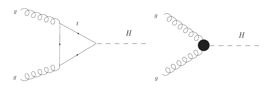
Figure 4: Born Level diagrams for Higgs boson production in $gg$ channel, respectively in the full (left) and effective theory (right).

Here we will only consider the case of the effective field theory: we first determine the full resummed result, and then we expand it out up to $\mathcal{O}(\alpha_{s}^{4})$. This illustrates our methodology, it provides a nontrivial check of it, and yields a prediction for the next fixed order.

As explained in the previous section, in order to determine the $p_{\rm\scriptscriptstyle\rm T}$-dependent impact factor $h_{p_{\rm\scriptscriptstyle\rm T}}$, Eq. (3), we must determine the transverse momentum distribution $C_{p_{\rm\scriptscriptstyle\rm T}}$ for the process

$$g^{*}\left(p_{L}\right)+g^{*}\left(n_{L}\right)\to H\left(p_{\mathcal{S}}\right)$$ (4.1)

with incoming off-shell gluons. The color-averaged squared matrix element in the effective theory is Hautmann:2002tu ; Marzani:tesi

$$\left|\,\mathcal{M}\,\right|^{2}=\frac{\alpha_{s}^{2}}{32}\frac{\sqrt{2}G_{\scriptscriptstyle\rm F}}{9\pi^{2}}\frac{\left(\mathbf{k}\cdot\mathbf{\bar{k}}\right)^{2}}{\left|\,\mathbf{k}\,\right|^{2}\left|\,\mathbf{\bar{k}}^{2}\,\right|}\left(\frac{m_{\scriptscriptstyle\rm H}^{2}}{\tau}\right)^{2}$$ (4.2)

where ${\bf k}$ and ${\bf\bar{k}}$ are respectively the transverse components of $p_{L}$ and $n_{L}$ Eq. (2.6), and $\tau=\frac{x}{z\bar{z}}$.

The coefficient function $C_{p_{\rm\scriptscriptstyle\rm T}}$ is found by providing necessary phase space factor, and performing a Mellin transform:

$$C_{p_{\rm\scriptscriptstyle\rm T}}\left(N,\xi,\bar{\xi},\xi_{p},\alpha_{s}\right)=\frac{\alpha_{s}^{2}\sqrt{2}G_{\scriptscriptstyle\rm F}}{288\pi}\int_{0}^{1}d\tau\,\tau^{N-1}\int_{0}^{2\pi}\frac{d\theta}{2\pi}\frac{\cos^{2}\theta}{\tau}\,\delta\left(\frac{1}{\tau}-1-\xi_{p}\right)$$

$$\qquad\qquad\qquad\delta\left(\xi_{p}-\xi-\bar{\xi}-2\sqrt{\xi\bar{\xi}}\cos\theta\right)$$

$$\quad=2\sigma_{\scriptscriptstyle\rm\rm LO}\;\,\int_{0}^{1}d\tau\,\tau^{N-2}\,\delta\bigg{(}\frac{1}{\tau}-1-\xi_{p}\bigg{)}\int_{0}^{2\pi}\frac{d\theta}{2\pi}\cos^{2}\theta\,\delta\left(\xi_{p}-\xi-\bar{\xi}-2\sqrt{\xi\bar{\xi}}\cos\theta\right)$$ (4.3)

where $\xi$, $\bar{\xi}$ and $\xi_{p}$ were defined in Eqs. (2.21-3.4) and

$$\sigma_{\scriptscriptstyle\rm\rm LO}=\frac{\alpha_{s}^{2}\sqrt{2}G_{\scriptscriptstyle\rm F}}{576\pi}$$ (4.4)

is the leading-order inclusive cross-section.

The integrals in $\tau$ and $\theta$ in Eq. (4) can be performed explicitly, with the result

$$h_{p_{\rm\scriptscriptstyle\rm T}}\left(N,M_{1},M_{2},\xi_{p},\alpha_{s}\right)=\frac{\sigma_{\scriptscriptstyle\rm\rm LO}}{2\pi\left(1+\xi_{p}\right)^{N}}M_{1}M_{2}R\left(M_{1}\right)R\left(M_{2}\right)$$

$$\qquad\qquad\int_{0}^{\infty}d\xi\,\xi^{M_{1}-2}\int_{\left(\sqrt{\xi_{p}}-\sqrt{\xi}\right)^{2}}^{\left(\sqrt{\xi_{p}}+\sqrt{\xi}\right)^{2}}d\bar{\xi}\,\bar{\xi}^{M_{2}-2}\frac{\left(\xi_{p}-\xi-\bar{\xi}\right)^{2}}{\sqrt{2\bar{\xi}\xi+2\xi\xi_{p}+2\bar{\xi}\xi_{p}-\xi_{p}^{2}-\xi^{2}-\bar{\xi}^{2}}}.$$ (4.5)

Changing variables

$$\xi=\xi_{p}\,\xi_{1},\qquad\bar{\xi}=\xi_{p}\,\xi_{2},$$ (4.6)

the dependence on $\xi_{p}$ can be taken outside the integral in Eq. (4):

$$h_{p_{\rm\scriptscriptstyle\rm T}}\left(N,M_{1},M_{2},\xi_{p},\alpha_{s}\right)=\sigma_{\scriptscriptstyle\rm\rm LO}\frac{\xi_{p}^{M_{1}+M_{2}-1}}{\left(1+\xi_{p}\right)^{N}}I\left(M_{1},M_{2}\right),$$ (4.7)

and the integral

$$I\left(M_{1},M_{2}\right)=M_{1}M_{2}\,R\left(M_{1}\right)R\left(M_{2}\right)$$ (4.8)

$$\qquad\int_{0}^{\infty}d\xi_{1}\,\xi_{1}^{M_{1}-2}\,\int_{\left(1-\sqrt{\xi_{1}}\right)^{2}}^{\left(1+\sqrt{\xi_{1}}\right)^{2}}d\xi_{2}\,\xi_{2}^{M_{2}-2}\frac{\left(1-\xi_{1}-\xi_{2}\right)^{2}}{\sqrt{2\xi_{1}\xi_{2}+2\xi_{1}+2\xi_{2}-1-\xi_{1}^{2}-\xi_{2}^{2}}}$$ (4.9)

does not depend on $\xi_{p}$.

The integrals over $\xi_{1}$ and $\xi_{2}$ in $I$ are computed in Appendix A; substituting the result [Eq. (A.7)] in Eq. (4.7) we finally find that the impact factor is given by

$$h_{p_{\rm\scriptscriptstyle\rm T}}\left(N,M_{1},M_{2},\xi_{p},\alpha_{s}\right)=R\left(M_{1}\right)R\left(M_{2}\right)\sigma_{\scriptscriptstyle\rm\rm LO}\frac{\xi_{p}^{M_{1}+M_{2}-1}}{\left(1+\xi_{p}\right)^{N}}$$

$$\qquad\left[\frac{\Gamma\left(1+M_{1}\right)\Gamma\left(1+M_{2}\right)\Gamma\left(2-M_{1}-M_{2}\right)}{\Gamma\left(2-M_{1}\right)\Gamma\left(2-M_{2}\right)\Gamma\left(M_{1}+M_{2}\right)}\left(1+\frac{2M_{1}M_{2}}{1-M_{1}-M_{2}}\right)\right].$$ (4.10)

The fact that the $\xi_{p}$ dependence is entirely contained in a prefactor is a consequence of the fact that in the effective theory the interaction is pointlike, and thus the transverse momentum dependence is entirely due to collinear radiation, as discussed in the end of Sect. 3. The resummed result is found from Eq. (4) by letting $N=0$ and by substituting for $M_{i}$ the LL$x$ anomalous dimension Eq. (3.10), according to Eq. (3). Our result manifestly reproduces the expected all-order behaviour Eq. (3.18).

We may check that integration of the transverse momentum dependent impact factor reproduces the known inclusive result: using the integral

$$\int_{0}^{\infty}d\xi_{p}\frac{\xi_{p}^{M_{1}+M_{2}-1}}{\left(1+\xi_{p}\right)^{N}}=\frac{\Gamma\left(M_{1}+M_{2}\right)\Gamma\left(N-M_{1}-M_{2}\right)}{\Gamma\left(N\right)}$$ (4.11)

in Eq. (4) we obtain the inclusive impact factor as given in Eq. (5.33) of Ref. Marzani:tesi .

We can now expand our result in powers of $\alpha_{s}$ in order to compare to known fixed-order expressions. We get

$$\frac{d\sigma}{d\xi_{p}}\left(N,\alpha_{s}\right)=\sigma_{LO}\sum_{k=1}^{\infty}C_{k}\left(\xi_{p}\right)\alpha_{s}^{k}\frac{\ln^{k-1}x}{k-1!}$$ (4.12)

with

$$C_{1}\left(\xi_{p}\right)= \frac{2C_{\rm\scriptscriptstyle\rm A}}{\pi}\frac{1}{\xi_{p}}$$ (4.13a)

$$C_{2}\left(\xi_{p}\right)= \frac{4C_{\rm\scriptscriptstyle\rm A}^{2}}{\pi^{2}}\frac{\ln\xi_{p}}{\xi_{p}}$$ (4.13b)

$$C_{3}\left(\xi_{p}\right)= \frac{2C_{\rm\scriptscriptstyle\rm A}^{3}}{\pi^{3}}\frac{1+2\ln^{2}\xi_{p}}{\xi_{p}}$$ (4.13c)

$$C_{4}\left(\xi_{p}\right)= \frac{4C_{\rm\scriptscriptstyle\rm A}^{4}}{\pi^{4}}\frac{3+3\ln\xi_{p}+2\ln^{3}\xi_{p}+17\zeta_{3}}{3\xi_{p}}.$$ (4.13d)

Equation (4.12) gives the result in the gluon channel; results in channels involving quarks can be obtained using Eq. (3.15).

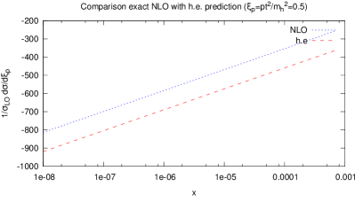
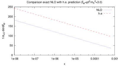
Figure 5: NLO contribution to the transverse momentum distribution for Higgs production in gluon fusion, normalized to $\sigma_{LO}$, compared to the high energy prediction $C_{2}\left(\xi_{p}\right)$ Eq. (4.13b) for two different fixed values of $\xi_{p}=0.5$ and $\xi_{p}=3.0$ .

Comparison to the LO exact result can be performed analytically. The LO double-differential transverse momentum and rapidity distribution in the effective field theory in the gluon-gluon channel is given by Ellis:1987xu ; Baur:1989cm

$$\frac{d\sigma^{(0)}}{d\xi_{p}dy}\left(x,\xi_{p},y\right)=\sigma_{LO}\frac{\alpha_{s}C_{\rm\scriptscriptstyle\rm A}}{2\pi}x\frac{x^{4}+1+\left(\frac{t}{s}\right)^{4}+\left(\frac{u}{s}\right)^{4}}{\frac{ut}{s^{2}}}\delta\left(1+\frac{t}{s}+\frac{u}{s}-x\right),$$ (4.14)

where

$$x= \frac{m_{\scriptscriptstyle\rm H}^{2}}{s}$$ (4.15)

$$\frac{t}{s}= x-\sqrt{x}\sqrt{1+\xi_{p}}e^{y}$$ (4.16)

$$\frac{u}{s}= x+\sqrt{x}\sqrt{1+\xi_{p}}e^{-y}.$$ (4.17)

Integrating over rapidity we get

$$\frac{d\sigma^{(0)}}{d\xi_{p}}\left(x,\xi_{p},\alpha_{s}\right)=\alpha_{s}\sigma_{LO}\frac{2C_{\rm\scriptscriptstyle\rm A}}{\pi}\frac{1}{\xi_{p}}+\mathcal{O}\left(x\right)$$ (4.18)

in agreement with Eq. (4.12).

At NLO we compare to the full result numerically. The lengthy analytic expression for the double differential distribution is given in Ref. Glosser:2002gm . We have integrated this numerically over rapidity $y$, retaining the full $x$ dependence: this is necessary because, as discussed in Ref. Caola:2010kv , terms which appear to be power-suppressed in $x$ at the level of rapidity distribution lead to LL$x$ contributions upon integration.

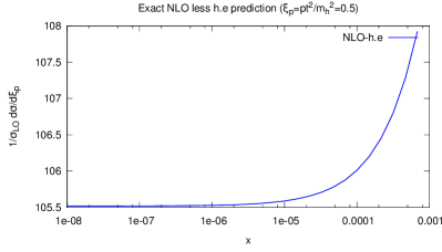
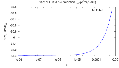
Figure 6: Difference between the NLO fixed order result and the high energy prediction $C_{2}\left(\xi_{p}\right)$ Eq. (4.13b) shown in Fig. 5.

The result of the integration is plotted as a function of $\ln x$ in Fig. 5, in the small $x$ region (blue line), together with the high-energy prediction Eq. (4.13b), for two values of the transverse momentum $p_{\rm\scriptscriptstyle\rm T}^{2}$. The difference between the two curves is shown in Fig. 6. It is clear that the difference between the two curves tends to a constant as $x\to 0$, thus proving perfect agreement between the high-energy behaviour and the exact result. We have repeated the comparison for a large number of values of $\xi_{p}$, with the same result. We have performed similar comparisons in the $gq$ and $q\bar{q}$ channels, and find similarly good agreement.

A test at NNLO is nontrivial due to the complexity of the exact result of Ref. Boughezal:2015dra which hampers its accurate numerical evaluation in the high energy limit; it is very likely to be possible thanks to the recent results of Ref. Banfi:2015pju . However, the NNLO coefficient can be tested by comparing to NNLL transverse momentum resummation, as we discuss in the next section.

5 Relation to transverse momentum resummation

As we have argued on general grounds in Sect. 3, Eq. (3.18), and seen explicitly in the case of Higgs in gluon fusion in Sect. 4, Eq. (4) the high-energy transverse momentum distribution in the pointlike limit displays an all-order single-logarithmic behaviour in $\xi_{p}$. On the other hand, in the $p_{\rm\scriptscriptstyle\rm T}\to 0$ limit (and not necessarily at high energy) by standard Wilson expansion arguments, the interaction can always be represented by a local operator and the effect of any other scale (such as the heavy quark masses) is entirely contained in a Wilson coefficient.

Therefore, in the high energy limit, the behaviour Eq. (3.18) (seen in Eq. (4)) always holds when $p_{\rm\scriptscriptstyle\rm T}\to 0$ i.e. when $\xi_{p}\to 0$, even in the resolved case, up to a prefactor (coming from the Wilson coefficient) which in our LL$x$ limit is independent of $\alpha_{s}$ and only depends on the scales which are integrated out in the effective field theory (e.g., in the case discussed in the previous section on the ratios of the heavy quark masses to the Higgs mass).

In this limit, however, hard cross sections are known to display double logs of the form $\frac{\ln^{2k-1}\xi_{p}}{\xi_{p}}$, which can be resummed using now standard techniques Collins:1984kg : in particular, N^kLL resummation allows one to predict the coefficients of all contributions of the form $\alpha_{s}^{n}\,\frac{\ln^{k}\xi_{p}}{\xi_{p}}$ with $2(n-k)-1\leq k\leq 2n-1$ In the high energy limit, the hard cross section displays single logs $\alpha_{s}^{n}\,\frac{\ln^{n}\xi_{p}}{\xi_{p}}$ Eq. (3.18) . It follows that at $\mathcal{O}(\alpha_{s}^{n})$ the coefficient of the highest power of $\ln\xi_{p}$ is predicted by N^n-1LL transverse momentum resummation, with lower-order powers of $\ln\xi_{p}$ predicted by increasingly subleading log resummation. In particular, the coefficients of $\ln^{2}\xi_{p}$ and $\ln\xi_{p}$ in $C_{3}$ Eq. (4.13c) are predicted by NNLL transverse momentum resummation, thereby allowing us to also check this coefficient.

The LL$x$ result in the $\xi_{p}\to 0$ limit, when taken to all orders in $\alpha_{s}$, thus provides information on N^kLL transverse momentum resummation to all logarithmic orders $0\leq k\leq\infty$ in the $x\to 0$ limit. An immediate consequence of this is that the structure of transverse momentum resummation must be reproduced in the high-energy limit. This structure was fully elucidated only recently in Refs. Catani:2000vq ; Catani:2011kr ; Catani:2013tia : schematically, the contributions to the partonic cross section which are singular as $p_{\rm\scriptscriptstyle\rm T}\to 0$ have the form

$$\frac{d\sigma^{\rm res}_{a_{1}a_{2}}}{d{\bf p_{\rm\scriptscriptstyle\rm T}}}\left(N,{\bf p_{\rm\scriptscriptstyle\rm T}},Q^{2}\right)=\sum_{ij}\sigma^{(0)}_{ij}\int d^{2}{\bf b}e^{i{\bf b}\cdot{\bf p_{\rm\scriptscriptstyle\rm T}}}S_{ij}(b^{2},Q^{2})$$

$$\quad\times\sum_{lm}\left[H_{ij,lm}(\alpha_{s})C_{il}(N,{\bf b})C_{jm}(N,{\bf b})+\bar{H}_{ij,lm}(\alpha_{s})G_{il}(N,{\bf b})G_{jm}(N,{\bf b})\right]\times$$ (5.1)

$$\qquad\times\Gamma_{la_{1}}[\alpha_{s},b^{2},Q^{2}]\Gamma_{ma_{2}}[\alpha_{s},b^{2},Q^{2}],$$

where $b=|{\bf b}|$; the sums over $(i,j)$ and $(l,m)$ run over parton channels (quark and gluon), $\Gamma_{i}$ are standard QCD evolution factors from scale $b$ to the hard scale $Q$ for the two incoming partons $a_{1}$ $a_{2}$; $S_{ij}$ is a Sudakov evolution factor; and all the process dependence is contained in the $N$-independent hard functions $H$ and $\bar{H}$ while the partonic functions $C_{il}$ and $G_{il}$ on the two incoming legs are universal. In the particular case of quark-initiated channel, the $G_{il}$ functions vanish.

Equation (5) imposes on our resummed result the nontrivial restriction that, in the $\xi_{p}\to 0$ limit, the dependence on $M_{1}$, $M_{2}$ of the impact factor Eq. (3) factorized, in the sense that it can be written as a sum which reproduces the schematic structure $C(M_{1})C(M_{2})+G(M_{1})G(M_{2})$ of the term in square brackets of Eq. (5). This behaviour should hold in the small $\xi_{p}$ limit in general, and, for pointlike interactions, for all $\xi_{p}$.

Having understood the general structure of the constraints imposed by the matching of transverse momentum resummation and high-energy resummation, we can now check explicitly whether they are satisfied by our resummed results. In order to verify whether the structure Eq. (5) is reproduced we must perform a Fourier transform of the resummed cross-section. To this purpose, we define a $b$-space impact factor

$$h_{p_{\rm\scriptscriptstyle\rm T}}\left(N,M_{1},M_{2},b,\alpha_{s}\right)=\int_{0}^{\infty}d\xi_{p}\,J_{0}(\sqrt{\xi_{p}}\,b\,m_{h})\,h_{p_{\rm\scriptscriptstyle\rm T}}\left(N,M_{1},M_{2},\xi_{p},\alpha_{s}\right).$$ (5.2)

The $b$-space cross-section is obtained by performing the usual identification Eq. (3.11) with the impact factor Eq. (5.2).

We get

$$h_{p_{\rm\scriptscriptstyle\rm T}}\left(0,M_{1},M_{2},b,\alpha_{s}\right)=\sigma_{0}e^{-(M_{1}+M_{2})\ln\frac{b^{2}m_{h}^{2}}{4}}R\left(M_{1}\right)R\left(M_{2}\right)$$

$$\qquad\times\left[\frac{\Gamma\left(1+M_{1}\right)}{\Gamma\left(1-M_{1}\right)}\frac{\Gamma\left(1+M_{2}\right)}{\Gamma\left(1-M_{2}\right)}+M_{1}\frac{\Gamma\left(1+M_{1}\right)}{\Gamma\left(2-M_{1}\right)}M_{2}\frac{\Gamma\left(1+M_{2}\right)}{\Gamma\left(2-M_{2}\right)}\right].$$ (5.3)

We recognize the structure Eq. (5): the exponential prefactor corresponds to the evolution factors $\Gamma_{i}$, as it is clear recalling that $M_{i}$ are set equal to the anomalous dimensions while at LL$x$ level $\alpha_{s}$ does not run, and the term in square brackets reproduces the correct structure of the universal partonic functions $C$ and $G$ of Eq. (5). Note that the hard function and the Sudakov factor in Eq. (5) do not depend on $N$; therefore, in the high energy limit at LL$x$ only their trivial $O(\alpha_{s}^{0})$ part contributes.

We thus see that indeed for pointlike interactions the structure of the result Eq. (5), as determined by transverse momentum resummation, hold in fact for all $\xi_{p}$ and not just in the small $p_{\rm\scriptscriptstyle\rm T}$ limit. On the other hand, we expect that in the small $p_{\rm\scriptscriptstyle\rm T}$ limit the result found in the full theory with exact top mass dependence will also reduce to the form Eq. (5).

Having verified that our result has the correct structure fixed by transverse momentum resummation constraints, we can check explicitly the coefficients $C_{i}$ Eqs. (4.13). Using the explicit expression of NNLL resummation for Higgs production Bozzi:2005wk in the small $x$ limit we get

$$\frac{d\sigma}{d\xi_{p}}\left(N,\xi_{p},\alpha_{s}\right)=\sigma_{LO}\left(1+\alpha_{s}^{2}\frac{C_{\rm\scriptscriptstyle\rm A}^{2}}{N^{2}}\right)\int_{0}^{\infty}db\,\frac{b}{2}\,J_{0}\left(\sqrt{\xi_{p}}\,b\,m_{h}\right)\exp\left[G^{h.e.}\left(N,L\right)\right]$$ (5.4)

with

$$G^{h.e.}\left(N,L\right)=\frac{2C_{\rm\scriptscriptstyle\rm A}}{N}\frac{\alpha_{s}}{\pi}L,$$ (5.5)

where

$$L\equiv L(b)=\ln b^{2}m_{h}^{2}.$$ (5.6)

Expanding the exponential and performing the Fourier transform in Eq. (5.4) we immediately reproduce the coefficients $C_{1}$, $C_{2}$, and the logarithmic contribution to $C_{3}$. We have explicitly checked that the same holds in quark channels. We conclude that our result is consistent with known results from transverse momentum resummation.

6 Outlook

We have shown that transverse momentum distributions can be resummed in the high energy limit in the same way as total cross-sections and rapidity distributions, namely, by computing the corresponding Born-level cross-section, but with incoming off-shell gluons. The extra complexity due to the transverse momentum dependence is entirely contained in the kinematic constraints which relates the transverse momentum of the final state to the off-shellness of the initial state, which is in turn re-expressed through high-energy factorization in terms of the so-called BFKL, or LL$x$ anomalous dimension.

Because of its relative simplicity, our result provides a powerful tool to obtain high-order information on collider processes. As a first demonstration we have considered here the case of Higgs production in gluon fusion in the pointlike limit. This is an interesting case both for validation and conceptual reasons, because full results are available to rather high perturbative orders, and also because the pointlike limit, though displaying unphysical double log behaviour at high energy, has a transverse momentum dependence which can be related to that which is revealed in small transverse momentum resummation.

On the other hand, matching high energy to transverse momentum resummation, both in the pointlike case and for the full theory, raises the interesting question of combining the two resummations marzaniprep . However, it should be kept in mind that for accurate phenomenology resummed results would have to be combined with the running coupling resummation at high energy discussed in Refs. Ball:2007ra ; Altarelli:2008aj .

On the other hand, the application of our technique to Higgs production in gluon fusion when the full dependence on the top mass is retained appears to be especially interesting as a way to gain information on higher order corrections. Indeed, only the leading order result is known in this case, while the pointlike approximation is known DelDuca:2001fn to fail badly for large values of the transverse momentum. Also, the structure of the dependence of this process on the various scales which characterize it (the heavy quark masses, the Higgs mass, and transverse momentum) is non-trivial and the object of ongoing investigations Banfi:2013eda ; Bagnaschi:2015bop . We expect our results, though partial, to help in shedding light on these issues, and work on this is currently ongoing.

Acknowledgements: We are grateful to S. Marzani for innumerable enlightening discussions and for raising the issue of the relation to transverse momentum resummation, and to F. Caola and G. Zanderighi for useful comments. We thank R. D. Ball, S. Marzani and especially F. Caola for a critical reading of the manuscript. This work is supported in part by an Italian PRIN2010 grant and by the Executive Research Agency (REA) of the European Commission under the Grant Agreement PITN-GA-2012-316704 (HiggsTools).

Appendix A The Higgs $p_{\rm\scriptscriptstyle\rm T}$-impact factor in the $m_{\rm\scriptscriptstyle\rm top}\to\infty$ limit

We provide here details on the computation of the double Mellin transform integral Eq. (4.8) which leads to the final expression of the impact factor. We first change variables from $\xi_{2}$ to a new variable $u$, defined implicitly as

$$\xi_{2}=1+\xi_{1}-2\sqrt{\xi_{1}}u$$ (A.1)

in terms of which, Eq. (4.8) becomes

$$I\left(M_{1},M_{2}\right)= M_{1}M_{2}R\left(M_{1}\right)R\left(M_{2}\right)$$

$$\int_{0}^{\infty}d\xi_{1}\,4\xi_{1}^{M_{1}}\int_{-1}^{1}du\,\left(1-\frac{1}{\sqrt{\xi_{1}}}u\right)^{2}\left(1+\xi_{1}\right)^{M_{2}-2}\frac{\left(1-\sqrt{r}u\right)^{M_{2}-2}}{\sqrt{1-u^{2}}},$$ (A.2)

where $r\equiv\frac{4\xi_{1}}{\left(1+\xi_{1}\right)^{2}}$.

With straightforward manipulations, Eq. (A) can be rewritten in terms of a single integral function

$$F\left(M_{1},M_{2}\right)=\int_{0}^{\infty}d\xi_{1}\,\xi_{1}^{M_{1}}\left(1+\xi_{1}\right)^{M_{2}}\int_{-1}^{1}du\,\frac{\left(1-\sqrt{r}u\right)^{M_{2}}}{\sqrt{1-u^{2}}},$$ (A.3)

as

$$I\left(M_{1},M_{2}\right)= M_{1}M_{2}R\left(M_{1}\right)R\left(M_{2}\right)$$

$$\Big{[}F\left(M_{1}-2,M_{2}-2\right)-2F\left(M_{1}-1,M_{2}-2\right)+F\left(M_{1},M_{2}-2\right)$$

$$-2F\left(M_{1}-2,M_{2}-1\right)+2F\left(M_{1}-1,M_{2}-1\right)+F\left(M_{1}-2,M_{2}\right)\Big{]}.$$ (A.4)

We compute $F$ by expanding $\left(1-\sqrt{r}u\right)^{M_{2}}$ in powers of $u$, with the result

$$F\left(M_{1},M_{2}\right)= \int_{0}^{\infty}d\xi_{1}\,\xi_{1}^{M_{1}}\left(1+\xi_{1}\right)^{M_{2}}\int_{-1}^{1}du\,\frac{\left(1-\sqrt{r}u\right)^{M_{2}}}{\sqrt{1-u^{2}}}$$

$$= \sum_{k=0}^{\infty}\binom{M_{2}}{2k}\int_{0}^{\infty}d\xi_{1}\,\xi_{1}^{M_{1}}\left(1+\xi_{1}\right)^{M_{2}}r^{k}\int_{-1}^{1}du\,\frac{u^{2k}}{\sqrt{1-u^{2}}}$$

$$= \sum_{k=0}^{\infty}\binom{M_{2}}{2k}\frac{4^{k}\sqrt{\pi}\Gamma\left(\frac{1}{2}+k\right)}{\Gamma\left(1+k\right)}\int_{0}^{\infty}d\xi_{1}\,\xi_{1}^{M_{1}+k}\left(1+\xi_{1}\right)^{M_{2}-2k}$$

$$= \sum_{k=0}^{\infty}\binom{M_{2}}{2k}\frac{4^{k}\sqrt{\pi}\Gamma\left(\frac{1}{2}+k\right)}{\Gamma\left(1+k\right)}\frac{\Gamma\left(1+k+M_{1}\right)\Gamma\left(k-1-M_{1}-M_{2}\right)}{\Gamma\left(2k-M_{2}\right)}.$$ (A.5)

The sum can then be performed in closed form:

$$F\left(M_{1},M_{2}\right)=\frac{\pi\Gamma\left(1+M_{1}\right)\Gamma\left(1+M_{2}\right)\Gamma\left(-1-M_{1}-M_{2}\right)}{\Gamma\left(-M_{1}\right)\Gamma\left(-M_{2}\right)\Gamma\left(2+M_{1}+M_{2}\right)}.$$ (A.6)

Substituting this expression in Eq. (A) and exploiting the properties of the Euler Gamma function we finally get

$$I\left(M_{1},M_{2}\right)=R\left(M_{1}\right)R\left(M_{2}\right)\left[\frac{\Gamma\left(1+M_{1}\right)\Gamma\left(1+M_{2}\right)\Gamma\left(2-M_{1}-M_{2}\right)}{\Gamma\left(2-M_{1}\right)\Gamma\left(2-M_{2}\right)\Gamma\left(M_{1}+M_{2}\right)}\left(1+\frac{2M_{1}M_{2}}{1-M_{1}-M_{2}}\right)\right].$$ (A.7)

References

(1)
S. Marzani, R. D. Ball, V. Del Duca, S. Forte and A. Vicini,
Nucl. Phys. B 800 (2008) 127
[arXiv:0801.2544 [hep-ph]].
(2)
R. V. Harlander, H. Mantler, S. Marzani and K. J. Ozeren,
Eur. Phys. J. C 66 (2010) 359
[arXiv:0912.2104 [hep-ph]].
(3)
S. Catani, M. Ciafaloni and F. Hautmann,
Phys. Lett. B 242 (1990) 97;
(4)
S. Catani, M. Ciafaloni and F. Hautmann,
Nucl. Phys. B 366 (1991) 135.
(5)
S. Catani and F. Hautmann,
Nucl. Phys. B 427 (1994) 475
[hep-ph/9405388].
(6)
R. D. Ball and R. K. Ellis,
JHEP 0105 (2001) 053
[hep-ph/0101199].
(7)
F. Hautmann,
Phys. Lett. B 535 (2002) 159
[hep-ph/0203140].
(8)
S. Marzani and R. D. Ball,
Nucl. Phys. B 814 (2009) 246
[arXiv:0812.3602 [hep-ph]].
(9)
G. Diana,
Nucl. Phys. B 824 (2010) 154
[arXiv:0906.4159 [hep-ph]].
(10)
F. Caola, S. Forte and S. Marzani,
Nucl. Phys. B 846 (2011) 167
[arXiv:1010.2743 [hep-ph]].
(11)
S. Dittmaier et al. [LHC Higgs Cross Section Working Group Collaboration],
doi:10.5170/CERN-2011-002
arXiv:1101.0593 [hep-ph].
(12)
U. Baur and E. W. N. Glover,
Nucl. Phys. B 339 (1990) 38.
(13)
R. Boughezal, F. Caola, K. Melnikov, F. Petriello and M. Schulze,
arXiv:1504.07922 [hep-ph].
(14)
F. Caola, “High-energy resummation in perturbative
QCD: theory and phenomenology”; Ph.D. Thesis, Milan University, July 2011
(15)
R. K. Ellis, H. Georgi, M. Machacek, H. D. Politzer and G. G. Ross,
Nucl. Phys. B 152 (1979) 285.
(16)
G. Curci, W. Furmanski and R. Petronzio,
Nucl. Phys. B 175 (1980) 27.
(17)
L. N. Lipatov, Sov. J. Nucl. Phys. 23 (1976) 338
[Yad. Fiz 23 (1976) 642].
V. S. Fadin, E. A. Kuraev, L. N. Lipatov, Phys. Lett. B 60 (1975) 50.
E. A. Kuraev, L. N. Lipatov, V. S. Fadin, Sov. Phys. JETP 44 (1976) 443 [Zh. Eksp. Teor. Fiz. 71 (1977) 840].
E. A. Kuraev, L. N. Lipatov, V. S. Fadin, Sov. Phys. JETP 45 (1977) 199 [Zh. Eksp. Teor. Fiz. 72 (1977) 377].
I. I. Balitsky, L. N. Lipatov, Sov. J. Nucl. Phys. 28 (1978) 822
[Yad. Fiz. 28 (1978) 1597].
(18)
R. D. Ball and S. Forte,
Phys. Lett. B 359, 362 (1995)
[hep-ph/9507321].
(19)
R. D. Ball and S. Forte,
Phys. Lett. B 405 (1997) 317
doi:10.1016/S0370-2693(97)00625-4
[hep-ph/9703417].
(20)
G. Altarelli, R. D. Ball and S. Forte,
Nucl. Phys. B 575 (2000) 313
[hep-ph/9911273].
(21)
C. J. Glosser and C. R. Schmidt,
JHEP 0212 (2002) 016
[hep-ph/0209248].
(22)
V. Ravindran, J. Smith and W. L. Van Neerven,
Nucl. Phys. B 634 (2002) 247
[hep-ph/0201114].
(23)
S. Marzani High Energy Resummation in Quantum Chromo
Dynamics, Ph.D. Thesis, Edinburgh University (2008)
https://www.era.lib.ed.ac.uk/handle/1842/3156
(24)
R. K. Ellis, I. Hinchliffe, M. Soldate and J. J. van der Bij,
Nucl. Phys. B 297 (1988) 221.
(25)
A. Banfi, F. Caola, F. A. Dreyer, P. F. Monni, G. P. Salam, G. Zanderighi and F. Dulat,
arXiv:1511.02886 [hep-ph].
(26)
J. C. Collins, D. E. Soper and G. F. Sterman,
Nucl. Phys. B 250 (1985) 199.
(27)
S. Catani, D. de Florian and M. Grazzini,
Nucl. Phys. B 596 (2001) 299
[hep-ph/0008184].
(28)
S. Catani and M. Grazzini,
Eur. Phys. J. C 72 (2012) 2013
[Eur. Phys. J. C 72 (2012) 2132]
[arXiv:1106.4652 [hep-ph]].
(29)
S. Catani, L. Cieri, D. de Florian, G. Ferrera and M. Grazzini,
Nucl. Phys. B 881 (2014) 414
[arXiv:1311.1654 [hep-ph]].
(30)
G. Bozzi, S. Catani, D. de Florian and M. Grazzini,
Nucl. Phys. B 737 (2006) 73
[hep-ph/0508068].
(31) S. Marzani, in preparation
(32)
R. D. Ball,
Nucl. Phys. B 796 (2008) 137
doi:10.1016/j.nuclphysb.2007.12.014
[arXiv:0708.1277 [hep-ph]].
(33)
G. Altarelli, R. D. Ball and S. Forte,
Nucl. Phys. B 799 (2008) 199
doi:10.1016/j.nuclphysb.2008.03.003
[arXiv:0802.0032 [hep-ph]].
(34)
V. Del Duca, W. Kilgore, C. Oleari, C. Schmidt and D. Zeppenfeld,
Nucl. Phys. B 616 (2001) 367
[hep-ph/0108030].
(35)
A. Banfi, P. F. Monni and G. Zanderighi,
JHEP 1401 (2014) 097
[arXiv:1308.4634 [hep-ph]].
(36)
E. Bagnaschi, R. V. Harlander, H. Mantler, A. Vicini and M. Wiesemann,
arXiv:1510.08850 [hep-ph].