Observational Searches for Star-Forming Galaxies at $z>$ 6

Abstract

Although the universe at redshifts greater than six represents only the first one billion years ($<$10%) of cosmic time, the dense nature of the early universe led to vigorous galaxy formation and evolution activity which we are only now starting to piece together. Technological improvements have, over only the past decade, allowed large samples of galaxies at such high redshifts to be collected, providing a glimpse into the epoch of formation of the first stars and galaxies. A wide variety of observational techniques have led to the discovery of thousands of galaxy candidates at $z>$ 6, with spectroscopically confirmed galaxies out to nearly $z=$ 9. Using these large samples, we have begun to gain a physical insight into the processes inherent in galaxy evolution at early times. In this review, I will discuss i) the selection techniques for finding distant galaxies, including a summary of previous and ongoing ground and space-based searches, and spectroscopic followup efforts, ii) insights into galaxy evolution gleaned from measures such as the rest-frame ultraviolet luminosity function, the stellar mass function, and galaxy star-formation rates, and iii) the effect of galaxies on their surrounding environment, including the chemical enrichment of the universe, and the reionization of the intergalactic medium. Finally, I conclude with prospects for future observational study of the distant universe, using a bevy of new state-of-the-art facilities coming online over the next decade and beyond.

1 INTRODUCTION

1.1 Probing our origins

A central feature of humanity is our inherent curiosity about our origins and those of the world around us. These two desires reach a crux with astronomy, where by studying the universe around us we also peer back into our own genesis. It is thus no surprise that an understanding of the emergence of our own Milky Way galaxy has long been a highly pursued field in astronomy. A number of observational probes into our Milky Way’s beginnings are available, from studying the stellar populations in our Galaxy (or nearby galaxies), stellar archaeology, and even primordial abundances in our Solar System.

The finite speed of light is a key property of nature that by delaying our perception of distant objects allows us to glimpse deep into the history of our Universe. A complementary approach is thus to directly study the likely progenitors of the Milky Way by peering back in time (e.g., Papovich et al. 2015). Over the past several decades, such studies have arrived at the prevailing theory that today’s galaxies formed via the process of hierarchical merging, where smaller galaxies combine over time to form larger galaxies (e.g., Searle & Zinn 1978; Blumenthal et al. 1984). With present-day technology, we can now peer back to within one billion years of the Big Bang, seeing galaxies as they were when the universe was less than 10% of its present-day age.

1.2 The first galaxies in the Universe

One key goal in the search for our origins is to uncover the first galaxies. In the present day universe, normal galaxies have typical stellar masses of log(M/M_⊙) $\sim$ 10-11 (for reference, the stellar mass of the Milky Way is $\sim$5 $\times$ 10¹⁰ M_⊙; e.g., Mutch et al. 2011). However, as stellar mass builds up with time, it is sensible to assume that early galaxies were likely less massive. To understand how small these first galaxies might be, we need to turn to simulations of the early universe to explore predictions for the first luminous objects.

The universe at a time $\sim$10⁸ years after the Big Bang ($z\sim$ 30) was a much different environment than today. The era of recombination had just ended, and the cosmic microwave background (CMB) was filling the universe at a balmy temperature of $\sim$ 85 K. At that time, baryonic matter, freed from its coupling with radiation, had begun to fall into the gravitational potentials formed by the previously collapsed dark matter halos. Simulations show that the first stars in the universe formed in dark matter halos with masses of $\sim$10⁶ M_⊙ (known as mini-halos; Couchman & Rees 1986; Tegmark et al. 1997). Stars forming in these halos were much different than those in the local universe, as the chemical composition in the universe prior to the onset of any star formation lacked any metals. As metals are a primary coolant in the local interstellar medium (ISM), gas in these minihalos must cool through different channels to reach the density threshold for star formation (e.g., Galli & Palla 1998). Even lacking metals, gas can still cool through hydrogen atomic line emission, but only in halos where the virial temperature is $>$10⁴ K. These “atomic cooling halos” have virial masses of $\gtrsim$ 10⁸ M_⊙, and are thus more massive than the likely host halos of the first stars.

In the absence of more advanced chemistry, small amounts of molecular hydrogen (H₂) were able to form in these minihalos, and these dense gas clouds were the sites of the formation of the first stars. Lacking the ability to cool to temperatures as low as present day stars, simulations have shown that the first stars were likely much more massive, with characteristic masses from $\sim$10 M_⊙ up to $>$ 100 M_⊙ (e.g., Bromm & Larson 2004; Glover 2005). These stars consisted solely of hydrogen and helium, and are thus referred to as Population III stars, compared to the metal-poor Population II, or metal-rich Population I stars.

However, these first objects were not galaxies, as the first simulations of such objects showed that most minihalos would form but a single Population III star (e.g., Bromm & Larson 2004). Subsequent simulations have shown that due to a variety of feedback effects (Lyman-Werner radiation, photoionization, X-ray heating, etc.), the collapsing gas may fragment and form a small star cluster. The most advanced ab initio simulations show this fragmentation, but they also show that some of these protostars merge back together (Greif et al. 2011). Given the computational cost involved in these latter simulations, they are not yet able to run until the stars ignite, thus it is unknown whether the final result is a single highly massive star, or a cluster of more moderate-mass stars. However, even in the latter case it is likely that the initial mass function has a higher characteristic mass than in the present day universe (e.g., Safranek-Shrader et al. 2014).

When the one (or more) massive stars in these mini-halos reach the end of their life and explode as a supernova, the energy injected may be enough to heat and expel much of the remaining gas, and suppress further star formation. Eventually, the now-enriched gas will fall back in, cool, and begin forming Population II stars. By this time, the dark matter halos have likely grown to be in the $\sim$ 10⁸ M_⊙ range, with the subsequent forming stellar masses likely $\gtrsim$10⁶ M_⊙. These “first galaxies” will ultimately be observable with the James Webb Space Telescope, and today, we can observe their direct descendants with stellar masses of $\sim$10^7-8 M_⊙ with deep Hubble Space Telescope (HST) surveys. The nature of these earliest observable galaxies is a key active area of galaxy evolution studies.

1.3 Reionization

The build up of galaxies in the early universe is deeply intertwined with the epoch of reionization, when the gas in the intergalactic medium (IGM), which had been neutral since recombination at $z\sim$ 1000, became yet again ionized. Although the necessary ionizing photons could in principle come from a variety of astrophysical sources, the prevailing theory is that galaxies provide the bulk of the necessary photons (e.g., Stiavelli et al. 2004; Richards et al. 2006; Robertson et al. 2010; Finkelstein et al. 2012a; Robertson et al. 2013; Finkelstein et al. 2015c; Robertson et al. 2015; Bouwens et al. 2015a, though see Giallongo et al. 2015; Madau & Haardt 2015 for a possible non-negligible contribution for accreting super-massive black holes). Thus, understanding both the spatial nature and temporal history of reionization provides a crucial insight into the formation and evolution of the earliest galaxies in the universe.

Current constraints from the CMB show that the optical depth to electron scattering along the line-of-sight is consistent with an instantaneous reionization redshift of 8.8${}_{-1.1}^{+1.2}$ (Planck Collaboration et al. 2015). However, reionization was likely a more extended process. Simulations show that reionization likely started as an inside-out process where overdense regions first formed large H ii regions, which then overlapped in a “swiss-cheese” phase, ultimately ending as an outside-in process, where the last remnants of the neutral IGM were ionized (e.g., Barkana & Loeb 2001; Iliev et al. 2006; Alvarez et al. 2009; Finlator et al. 2009). Current constraints from galaxy studies show that reionization likely ended by $z\sim$ 6, and may have started as early as $z>$ 10 (Finkelstein et al. 2015c; Robertson et al. 2015).

In addition to ionizing the diffuse IGM, reionization likely had an adverse impact on star formation in the smallest halos. Those halos which could not self-shield against the suddenly intense UV background would have all of their gas heated, unable to continue forming stars. This has a significant prediction for the faint-end of the high-redshift luminosity function – it must truncate at some point. Current observational constraints place this turnover at M${}_{\mathrm{UV}}>-$17, while theoretical results show it occurs likely somewhere in the range $-$13 $<$ M_UV $<-$10, though some simulations find that other aspects of galaxy physics may produce a turnover at $-$16 $<$ M_UV $<-$14 (Jaacks et al. 2013; O’Shea et al. 2015). Identifying this turnover is crucial for the use of galaxies as probes of reionization, as the steep faint-end slopes observed yield an integral of the luminosity function that can vary significantly depending on the faintest luminosity considered. Even JWST will not probe faint enough to see these galaxies (although with gravitational lensing it may be possible), but the burgeoning field of near-field cosmology aims to use local dwarf galaxies, which may be the descendants of these quenched systems, to provide further observational insight (e.g., Brown et al. 2014; Boylan-Kolchin et al. 2015; Graus et al. 2015).

With the ability to study the Universe so close to its beginning, it is natural to ask: when did the first galaxies appear, and what were their properties? This review will concern itself with our progress with answering this question, focusing on observational searches for galaxies at redshifts greater than six, building on the work of previous reviews of galaxies at 3 $<z<$ 6 of Stern & Spinrad (1999) and Giavalisco (2002). In §2 I discuss methods for discovering distant galaxies, while in §3 I highlight recent search results, and in §4 I discuss spectroscopic followup efforts. In §5 and §6, I discuss our current understanding of galaxy evolution at $z>$ 6, while in §7 I discuss reionization. I conclude in §8 by discussing the prospects towards improving our understanding over the next decade. Throughout this paper, when relevant, a Planck cosmology of H${}_{0}=$ 67.3, $\Omega_{m}=$ 0.315 and $\Omega_{\Lambda}=$ 0.685 (Planck Collaboration et al. 2015) is assumed.

2 Selection Techniques for Distant Galaxies

To understand galaxies in the distant universe, one needs a method to construct a complete sample of galaxies, with minimal contamination. The obvious course here is spectroscopy - with a deep, wide spectroscopic survey, one can construct a galaxy sample with high-confidence redshifts, particularly when the continuum and/or multiple emission lines are observed. This has been accomplished in the low-redshift universe, by, for example, the CfA Redshift Survey (Huchra et al. 1983), the 2dF Galaxy Redshift Survey (Colless et al. 2001), and the Sloan Digital Sky Survey (SDSS; e.g., Strauss et al. 2002). While still highly relevant surveys more than a decade after their completion, these studies are limited to $z\lesssim$ 0.5. Future spectroscopic surveys, such as the Hobby Eberly Telescope Dark Energy Experiment (HETDEX; Hill et al. 2008) and the Dark Energy Spectroscopic Instrument (DESI; Flaugher & Bebek 2014), will enhance the spectroscopic discovery space out to $z\sim$ 3. However, due to the extreme faintness of distant galaxies, the $z\sim$ 6 universe is largely presently out of reach for wide-field, blind spectroscopic surveys.

2.1 Spectral Break Selection

Succesful studies of the $z>$ 3 universe have thus turned to broadband photometry. Although the spectroscopic resolution of broadband filters is extremely low (R $\sim$ 5 for the SDSS filter set), photometry can still be used to discern strong spectral features. The intrinsic spectra of star-forming galaxies exhibit two relatively strong spectral breaks. The first is the Lyman break at 912 Å, which is the result of the hydrogen ionization edge in massive stars, combined with the photoelectric absorption of more energetic photons by neutral gas (H i) in the interstellar media (ISM) of galaxies. The second break due to a combination of absorption by the higher-order Balmer series lines down to the Balmer limit at 3646 Å (strongest in A-type stars), along with absorption from metal lines in lower mass stars, primarily the Ca H and K lines (3934 and 3969 Å), strongest in lower-mass, G-type stars. Although this so-called “4000 Å break” can become strong in galaxies dominated by older stellar populations, it is typically much weaker than the Lyman break, which can span an order of magnitude or more in luminosity density.

The intergalactic medium adds to the amplitude of the Lyman break, as neutral gas along the line of sight (either in the cosmic web, or in the circum-galactic medium of galaxies) efficiently absorbs any escaping ionizing radiation (with a rest-frame wavelength less than 912 Å). Additionally, the continuum of galaxy spectra between 912 and 1216 Å will be attenuated by Ly$\alpha$ absorption lines in discrete systems along the line-of-sight, known as the Lyman-$\alpha$ forest. This latter effect is redshift-dependent, in that at higher redshift, more opacity is encountered along the line-of-sight. By $z\gtrsim$ 5, the region between the Lyman continuum edge and Ly$\alpha$ is essentially opaque, such that no flux is received below 1216 Å, compared to 912 Å at lower redshifts. As such, the Lyman break is occasionally referred to as the Lyman-$\alpha$ break at higher redshifts, although the mechanism is generically similar.

At $z>$ 3, the Lyman break feature shifts into the optical, and can thus be accessed from large-aperture, wide-field ground-based telescopes. Building on the efforts of Tyson (1988), Guhathakurta et al. (1990) and Lilly et al. (1991), Steidel & Hamilton (1993) was among the first to realize this tremendous opportunity to study the distant universe. They used a set of three filters ($U_{n}$, $G$ and $\mathscr{R}$) devised a set of color criteria to select galaxies at $z\sim$ 3 in two fields around high-redshift quasars. At this redshift, the Lyman break occurs between the $U_{n}$ and $G$ bands, thus a red $U_{n}-G$ color (or, a high $G$/$U_{n}$ flux ratio) corresponds to a strong break in the spectral energy distribution (SED) of a given galaxy between these filters. While this alone can efficiently find galaxies with strong Lyman breaks, corresponding to redshifts of $z\sim$ 3, it may also select lower-redshift galaxies with red rest-frame optical continua. Thus a second color is used, $G-\mathscr{R}$, corresponding to the rest-frame UV redward of the Lyman break at $z\sim$ 3, with a requirement that this color is relatively blue, to exclude lower-redshift passive and/or dusty galaxies from contaminating the sample. I refer the reader to the review by Giavalisco (2002) for further details on Lyman break galaxies at $z<$ 6.

The Lyman break is the primary spectral feature used in nearly all modern searches for $z>$ 6 galaxies. In §3 below, I will discuss recent searches with this technique. Some studies continue to use a set of color criteria, typically involving three filters, qualitatively similar to Steidel & Hamilton (1993). However, a more recent technique is beginning to become commonplace, known as photometric redshift fitting. In this technique, one compares the colors of a photometric sample to a set of template SEDs in all available filters. The advantage here is that one uses all available information to discern a redshift. Additionally, most photometric redshift tools calculate the redshift probability distribution function, therefore giving a higher precision on the most likely redshift, typically with $\Delta$z $\sim\pm$0.2-0.3 at $z>$ 6, compared to $\Delta$z $\sim\pm$0.5 for the two-color selection technique. The disadvantage is that this technique is dependent on the set of SED templates assumed. However, at $z\sim$ 6 this worry is alleviated as the primary spectral feature dominating the photometric redshift calculation is the Lyman break, thus the effect of different template choices is likely minimized. In Figure 1, I show model spectra at three different redshifts, highlighting how the wavelength of the Lyman break, and its strength, changes with redshift, as well as example real galaxies at each of the redshifts shown. The right panel of Figure 1 also shows a color-color plot, highlighting how one could use the filter set from the left panel to perform a Lyman break selection. One note for the reader on terminology - frequently authors use the term “Lyman break galaxy” to denote a galaxy selected via the Lyman break technique. However, all distant galaxies, whether they are bright enough to be detected in a continuum survey or not, will exhibit a Lyman break. Thus, in this review I will use the term “continuum selected star-forming galaxies” to denote such objects, which are selected via either Lyman break color-color selection, or photometric redshift selection.

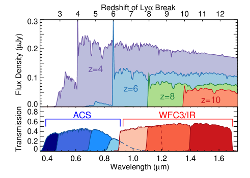
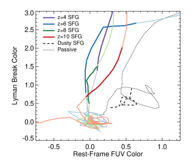
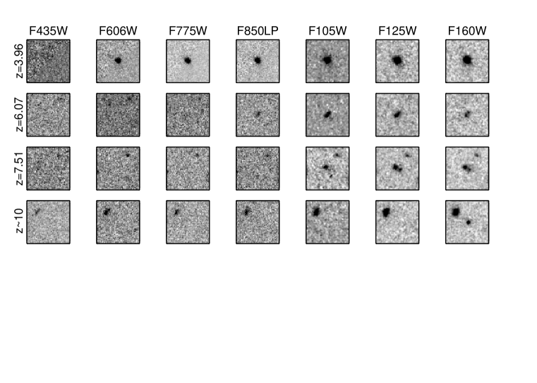
Figure 1: Top-Left) Model galaxy spectra at three different redshifts, compared to the Hubble Space Telescope optical (ACS) and near-infrared (WFC3) filter set available in the GOODS/CANDELS fields. The models shown have log (M/M_⊙) = 9, an age of 10⁸ yr, and $E(B-V)=$0.03. At $z>$ 7, the Lyman break shifts into the near-infrared, rendering such distant galaxies literally “invisible”. Top-Right) Color-color plot showing how the colors of normal star-forming galaxies (SFGs) at 4 $<z<$ 10 change with redshift. For the SFGs, the vertical axis represents the Lyman break color: $B-V$, $i^{\prime}-z^{\prime}$, $Y-J$ and $J-H$ at $z=$ 4, 6, 8 and 10, respectively. The horizontal axis represents the rest-frame far-ultraviolet color: $V-i^{\prime}$, $z^{\prime}-Y$, $J-H$ and $H-[3.6]$ at $z=$ 4, 6, 8 and 10, respectively. The dark portion of these curves represent when the curve is within $\Delta z\pm$ 0.5 of the center of the redshift bin. The dashed and dotted lines show the colors of dusty SFGs and passive galaxies from 0 $<z<$ 5, where for these we plot $z^{\prime}-Y$ versus $i^{\prime}-z^{\prime}$ (i.e., showing how these galaxies would compare to $z=$ 6 SFG colors). One can construct a box in each color-color combination which selects the desired high-redshift population, and excludes the low-redshift interlopers. Bottom) 3^′′ stamp images in the seven filters shown in the top-left panel centered on example galaxies at $z\sim$ 4, 6, 8 and 10 (the $z\sim$ 4, 6 and 8 galaxies are spectroscopically confirmed, and come from the sample of Finkelstein et al. 2015c, while the $z\sim$ 10 candidate galaxy comes from Bouwens et al. 2015b).

2.2 Emission Line Selection

Another method to select distant galaxies is via strong emission lines. At $z>$ 6, the only strong emission line accessible with current technology is the Lyman-$\alpha$ line, at $\lambda_{rest}=$ 1216 Å. While a blind spectroscopic survey for this feature is likely not practical at such high redshifts, this line is strong enough that it can be discerned with imaging in narrowband filters. A galaxy with a line at a particular wavelength covered by a narrowband filter will appear brighter in that narrowband then in a broadband filter covering similar wavelengths (as it will have a greater bandpass-averaged flux in the narrowband). This particular line was noted decades ago as a possible signpost for primordial star-formation in the early universe (Partridge & Peebles 1967), thus a variety of studies were commissioned with the goal of selecting large samples of Lyman-$\alpha$ emitting galaxies (LAEs). Although one of the first narrowband-selected LAEs was discovered by Djorgovski et al. (1985), it wasn’t until the advent of large aperture telescopes and/or wide-field optical imagers that the first large samples of LAEs were discovered (e.g. Cowie & Hu 1998; Rhoads et al. 2000).

LAEs form a complementary population of galaxies to continuum-selected star-forming galaxies. The study of Steidel & Hamilton (1993, and subsequent studies from that group) typically restricted their analyses to galaxies with observed optical AB magnitudes brighter than approximately 25, due to the limited depth available from ground-based broadband imaging. As narrowband selection techniques require only evidence of a large flux ratio between the narrowband and encompassing broadband filters, continuum detections are not required, and high equivalent width (EW) Ly$\alpha$ emission from galaxies with much fainter continuum levels can be detected. Deep broadband imaging of ground-based narrowband-selected LAEs shows that they are indeed on average fainter than continuum-selected galaxies, with continuum magnitudes as faint as $\sim$28 (for $z=$ 3–5 LAEs, e.g., Ouchi et al. 2008; Finkelstein et al. 2009). Whether LAEs form a completely separate population, or are simply the low-mass extension of the more massive continuum-selected galaxy population, remains an active area of study (e.g., Hashimoto et al. 2013; Nakajima et al. 2013; Song et al. 2014).

2.3 Infrared Selection

The previously discussed selection methods relied either on the detection of stellar continuum emission, or of nebular gas emission (due to photo-ionization from predominantly stellar-produced ionizing photons). An alternative method is also available, selecting galaxies based on the far-infrared emission from UV radiation re-processed by dust grains in the interstellar medium (e.g., Smail et al. 1997; Hughes et al. 1998; Barger et al. 1998). The advent of the Herschel Space Observatory as well as large-dish ground-based telescopes such as the James Clerk Maxwell Telescope (JCMT) with fast survey capabilities have allowed searches for rare, highly luminous dusty star-forming galaxies. The redshift distribution of such dusty star-forming galaxies peaks at $z\sim$ 2–3 (with the exact peak redshift depending on the selection-wavelength, with redder wavelengths selecting on average higher-redshift galaxies due to the redshifting of the dust-emission SED peak).

Surprisingly, the redshift distribution extends out to $z>$ 5 (see Casey et al. 2014, and references therein), implying that vast quantities of dust are produced in the early universe. Obtaining spectroscopic redshifts for such sources is difficult, as Ly$\alpha$ is easily attenuated by dust (though see, e.g., Barger et al. 1999; Chapman et al. 2005; Capak et al. 2008). However, the advent of the Atacama Large Millimeter Array (ALMA) now allows spectroscopic confirmation via a number of sub/millimeter lines, such as those on the CO ladder, or the [C ii] 158 $\mu$m fine structure line (e.g. Riechers et al. 2013). Although dust emission has been detected from galaxies as distant as $z\approx$ 7.5 (Watson et al. 2015), the vast majority of known dusty star-forming galaxies lie at $z<$ 6, thus I will not discuss these studies further in this review. However, ALMA, combined with a recent update to the Plateau du Bure interferometer (NOEMA), and a potential future update to the Jansky Very Large Array (NGVLA; Carilli et al. 2015), will further enable $z>$ 6 millimeter studies, and will soon provide key insight into such distant galaxies.

3 Surveys for High-Redshift Galaxies

In this section I discuss the results from recent surveys designed to discover galaxies at $z\geq$ 6. I will focus on the surveys and the galaxy samples, leaving the results from such studies for the subsequent sections.

3.1 Broadband Searches for Star-Forming Galaxies at $z=$ 6

Selecting galaxies at $z=$ 6 via the Lyman break technique requires imaging at the extreme red end of the optical, in the $z$-band at 0.9 $\mu$m, as galaxies at such redshifts are not visible at bluer wavelengths. Additionally, the imaging must be deep enough to detect these galaxies, as their increased luminosity distance results in an observed magnitude at $z=$ 6 that is $\sim$2 magnitudes fainter than a comparably intrinsically bright galaxy at $z=$ 2. Deep imaging in the $z$-band is difficult both due to the early lack of red-sensitive detectors, as well as (from the ground) the numerous night sky OH emission lines, which set a high background level. Although there were earlier examples of $z\approx$ 6 galaxies from, e.g., the Hubble Deep Field with WFPC2 (e.g., Weymann et al. 1998), larger samples of $z=$ 6 star-forming galaxies were not compiled until the installation of the red-sensitive optical Advanced Camera for Surveys (ACS) on HST in 2002. While initial studies using early observations found a handful of $z\sim$ 6 candidates (Bouwens et al. 2003; Stanway et al. 2003; Yan et al. 2003, including spectroscopic confirmations, e.g., Bunker et al. 2003), larger samples of more than 100 candidate $z=$ 6 galaxies were soon compiled using both the Great Observatories Origins Deep Survey (GOODS; Giavalisco et al. 2004a) and Hubble Ultra Deep Field (HUDF; Beckwith et al. 2006) datasets (Dickinson et al. 2004; Bunker et al. 2004; Giavalisco et al. 2004b; Bouwens et al. 2006).

Significant progress at $z=$ 6 has also been made from the ground. Although difficult due to the bright night sky emission, ground-based surveys can cover much larger areas, and thus provide complementary results on the bright-end of the galaxy luminosity function, which is difficult to constrain with HST due to the small field-of-view of HST’s cameras. Surveys such as the Subaru/XMM-Newton Survey (SXDS), the UKIRT Infrared Deep Sky Survey (UKIDDS)/Ultra Deep Survey (UDS), the Canada-France Hawaii Telescope Legacy Survey (CFHTLS), and the UltraVISTA Survey have searched areas of the sky from 1-4 deg² for $z=$ 6 galaxies (e.g., Kashikawa et al. 2006; McLure et al. 2009; Willott et al. 2013; Bowler et al. 2015). As discussed in §5, these wide-field surveys are necessary to probe luminosities much brighter than the characteristic luminosity at $z=$ 6.

One of the major conclusions from these early studies was that the galaxy population at $z=$ 6 could maintain an ionized IGM only if faint galaxies dominate the ionizing budget, which required that the luminosity function must maintain a steep faint-end slope well below L^∗ (e.g., Bunker et al. 2004; Yan & Windhorst 2004). Turning to the evolution of the cosmic star-formation rate (SFR) density, Giavalisco et al. (2004b) found that the evolution was remarkably flat out to $z=$ 6, such that the rate of cosmic star formation was similar at $z=$ 6 as at $z=$ 2. However, in a combined analysis using data from multiple HST surveys, Bouwens et al. (2007) found that there was a steep drop in the SFR density, by more than 0.5 dex from $z=$ 2 to 6. Some of this discrepancy may be due to the fact that many of these early $z=$ 6 galaxies were only detected in a single band, making robust samples (and their completeness corrections) difficult to construct, as well as hampering the ability to derive a robust dust-correction, which is necessary for an accurate measure of the SFR density.

This issue was alleviated with the installation of the Wide Field Camera 3 (WFC3) on HST in 2009, which contains both an ultraviolet/optical camera (WFC3/UVIS), and a near-infrared camera (WFC3/IR). Three major surveys were initiated with the infrared camera to probe high-redshift galaxies. The Hubble Ultra Deep Field 2009 survey (HUDF09; PI Illingworth) obtained deep imaging in three near-infrared filters (centered at 1, 1.25 and 1.6 $\mu$m) on the HUDF as well as two nearby parallel fields, while the Ultra Deep Field 2012 (UDF12; PI Ellis) survey increased the depth in these filters in the HUDF, and added a fourth filter at 1.4 $\mu$m. At the same time, the Cosmic Assembly Near-infrared Deep Extragalactic Legacy Survey (CANDELS; PIs Faber & Ferguson) was one of the three HST Multi-cycle Treasury Programs awarded in Cycle 18. CANDELS observed both GOODS fields in the same three WFC3/IR filters as the HUDF09 survey, as well as three additional fields (COSMOS; Extended Groth Strip/EGS, and Ultradeep Survey/UDS) in the 1.25 and 1.6$\mu$m filters. CANDELS also obtained optical imaging with ACS in parallel, which was particularly useful in the COSMOS, EGS and UDS fields, which had less archival ACS imaging than the GOODS fields. Using the combination of these new near-infrared data with the previously available ACS optical data, these data now allow full two-color selection of $z=$ 6 galaxies (Bouwens et al. 2015c) , as well as accurate photometric redshifts (Finkelstein et al. 2015c), for a sample of $\sim$700-800 robust candidates for $z=$ 6 galaxies.

3.2 Broadband Searches for Star-Forming Galaxies at $z\geq$ 7

At $z=$ 7, the Lyman break redshifts into the near-infrared, making deep near-infrared imaging a requirement. Prior to the advent of WFC3, the availability of the necessary imaging was scarce. Efforts were made with NICMOS imaging (e.g., Bouwens et al. 2010c), but with a survey efficiency $>$40$\times$ worse than WFC3 (a combination of depth and field size; Illingworth et al. 2013), significant progress in understanding early galaxy formation was difficult. The first large, robust samples of $z>$ 7 galaxies thus did not come about until the acquisition of the first year of the HUDF09 dataset. Several papers were published in the first few months after the initial Year 1 HUDF09 imaging (e.g., Oesch et al. 2010; Bouwens et al. 2010a; Bunker et al. 2010; McLure et al. 2010; Finkelstein et al. 2010), finding $\sim$10–20 robust $z=$ 7 candidate galaxies, as well as 5–10 $z=$ 8 candidate galaxies. Sample sizes of faint galaxies were increased with the completed two-year HUDF09 dataset, as well as the added depth from the UDF12 program (e.g., McLure et al. 2013; Schenker et al. 2013). The largest addition in sample size of $z=$ 7–8 galaxies was made possible by the CANDELS program, which, in the two GOODS fields alone, provided 5.4 and 3.7$\times$ more galaxies than the HUDF alone at $z=$ 7 and $z=$ 8, respectively (Finkelstein et al. 2015c). A large-area search for $z=$ 8 galaxies was also made possible by the Brightest of Reionizing Galaxies (BoRG) program, which used HST pure parallel imaging to find an additional $\sim$40 $z=$ 8 galaxy candidates at random positions in the sky. Recently, even larger samples of plausible $z=$ 7 and 8 galaxies were obtained by Bouwens et al. (2015c), who extended the search to all five CANDELS fields (as well as BoRG), making use of ground-based $Y$-band imaging in those regions without HST $Y$-band (i.e., the COSMOS, EGS and UDS CANDELS fields). The HST samples of $z=$ 7 and 8 galaxies now number $\sim$300-500 and $\sim$100-200, respectively.

Even at such great distances, ground-based searches have provided valuable data, particularly at $z=$ 7, though the bright night sky background still limits these studies to be restricted to relatively bright galaxies. Some of the first robust $z=$ 7 candidates discovered from the ground were published by Ouchi et al. (2009), who used ground-based near-infrared imaging over the Subaru Deep Field (SDF) and GOODS-N to select 22 $z=$ 7 candidate galaxies, all brighter than 26th magnitude, including some which are spectroscopically confirmed (Ono et al. 2012). Castellano et al. (2010) also used deep ground-based near-infrared imaging, here from the VLT/HAWK-I instrument, to find 20 candidate $z=$ 7 galaxies brighter than 26.7. Tilvi et al. (2013) took a complementary approach, using ground-based medium-band imaging to select three candidate $z=$ 7 galaxies from the zFourGE survey. Although the numbers discovered in this latter study were small, the higher spectral resolution afforded by the medium bands allows much more robust rejection of stellar contaminants, particularly brown dwarfs, which can mimic the broadband colors of $z\geq$ 6 galaxies (Figure 2). The most recent, and most constraining, ground-based results come from Bowler et al. (2012) and Bowler et al. (2014), who used deep, very wide-area imaging 1.65 deg² from the UltraVISTA COSMOS and the UKIDSS UDS surveys to discover 34 bright $z=$ 7 candidates. The combination of the very large area with the depth allowed Bowler et al. (2014) to have some overlap in luminosity dynamic range with the HST studies, which allows more robust joint constraints on the luminosity function.

Searches at even higher redshifts have been performed, with a number of studies now publishing candidates for galaxies at $z=$ 9 and 10. This is exceedingly difficult with HST alone, as at $z\gtrsim$ 8.8, galaxies will be detected in only the reddest two WFC3 filters (at 1.4 and 1.6 $\mu$m), while at $z\gtrsim$ 9.3, the Lyman break is already halfway through the 1.4 $\mu$m filter, rendering many higher redshift galaxies one-band (1.6 $\mu$m) detections. However, initial surveys did not include observations in the 1.4 $\mu$m band, thus only one-band detections were possible. These can be problematic, as one-band detections can pick up spurious sources such as noise spikes or oversplit regions of bright galaxies; the possibility of such a spurious source being detected in two independant images at the same locations is extremely low (see discussion in Schmidt et al. 2014 and Finkelstein et al. 2015c).

The first $z\geq$ 9 candidate galaxy published was a single $z\sim$ 10 object found in the HUDF by Bouwens et al. (2011a). The addition of 1.4 $\mu$m imaging in the HUDF by the UDF12 program led to further progress, with a handful of two-band detected $z\sim$ 9 candidate galaxies being discovered (Ellis et al. 2013; McLure et al. 2013; Oesch et al. 2013). Interestingly, the initial $z\sim$ 10 galaxy from Bouwens et al. (2011a) was not detected in this new 1.4$\mu$m imaging, implying that if it is truly at high redshift, it must be at $z\sim$ 12, although there is slight evidence that it may truly be an emission-line galaxy at z $\sim$ 2 (Brammer et al. 2013). Very high redshift galaxies have also been found via lensing from the CLASH and Hubble Frontier Fields programs, with candidates as high as $z\sim$ 11, although none have been spectroscopically confirmed (Coe et al. 2013; Zheng et al. 2012; Zitrin et al. 2014; Ishigaki et al. 2015; McLeod et al. 2015). More recent work by Oesch et al. (2014) and Bouwens et al. (2015c) have increased the sample sizes of plausible $z=$ 9 and 10 candidate galaxies by probing the full CANDELS area. Although extremely shallow 1.4 $\mu$m imaging is available (from pre-imaging for the 3D-HST program), these studies leverage the deep available Spitzer Space Telescope Infrared Array Camera (IRAC) imaging in these fields. These data cover 3.6 and 4.5 $\mu$m, which encompasses rest-frame 0.3–0.4 $\mu$m at $z=$ 9 and 10, and thus can potentially provide a second detection filter (though this is limited by the shallower depth and much broader point-spread function of the IRAC imaging). The latest results come from Bouwens et al. (2015b), which combine the results from Oesch et al. (2014) and Bouwens et al. (2015c) with new candidates from additional 1 $\mu$m imaging over selected galaxy candidates, finding a total sample of $\sim$15 and 6 robust candidate galaxies at $z=$ 9 and 10, respectively.

3.3 Narrowband Searches for Star-Forming Galaxies at $z\geq$ 6

There has also been an intensive effort to discover galaxies on the basis of strong Ly$\alpha$ emission with narrowband imaging surveys at $z>$ 6. These have been primarily ground-based, as the narrow redshift window probed combined with the small-area HST cameras renders space-based narrowband imaging inefficient. The narrowband technique has proven highly efficient at discovering large samples of LAEs at $z=$ 3–6 (e.g., Cowie & Hu 1998; Rhoads et al. 2000; Gawiser et al. 2006; Ouchi et al. 2008; Finkelstein et al. 2009), thus clearly an extension to higher redshift is warranted, though surveys at $z>$ 6 are restricted in redshift to wavelengths clear of night sky emission lines. The most complete survey for $z>$ 6 LAEs comes from Ouchi et al. (2010), who used the wide-area SuprimeCam instrument on the Subaru Telescope to discover $>$200 LAEs at $z=$ 6.6 over a square degree in the SXDS field. Matthee et al. (2015) have recently increased the area searched for LAEs at $z=$ 6.6 to five deg² over the UDS, SSA22 and COSMOS fields, finding 135 relatively bright LAEs.

Moving to higher redshift has proven difficult, as the quantum efficiency of even red-sensitive CCDs is declining. Nonetheless, Ota et al. (2010) imaged 0.25 deg² of the SXDS with SuprimeCam with a filter centered at 9730 Å, finding three candidate LAEs at $z=$ 7.0. Hibon et al. (2011) used the IMACS optical camera on the Magellan telescope to find six candidate $z=$ 6.96 LAEs in the COSMOS field, while Hibon et al. (2012) found eight candidate LAEs at $z=$ 7.02 in the SXDS with a 9755 Å narrowband filter on SuprimeCam. To observe LAEs at $z>$ 7 requires moving to the near-infrared, which has only recently been possible due to the advent of wide-format near-infrared cameras, such as NEWFIRM on the Kitt Peak 4m Mayall telescope. An additional complication is the increasing presence of night sky emission lines, which leaves few open wavelength windows, and drives many to use even narrower filters to mitigate the night sky emission as much as possible. One such window is at 1.06 $\mu$m, which corresponds to Ly$\alpha$ redshifted to $z=$ 7.7. At $z=$ 7.7, Hibon et al. (2010) used WIRCam on the CFHT to discover seven candidate LAEs, Krug et al. (2012) used NEWFIRM on the Kitt Peak 4m to discover four candidate LAEs, and Tilvi et al. (2010), also using NEWFIRM, found four additional candidate LAEs. However, the majority of these candidate LAEs remain undetected in accompanying broadband imaging, due primarily to the difficulty of obtaining deep broadband imaging in the near-infrared from the ground, and most also remain spectroscopically unconfirmed (e.g., Faisst et al. 2014), though see Rhoads et al. (2012) for one exception. Thus, the validity of the bulk of these sources is in question, and requires either deep (likely space-based) broadband imaging, or spectroscopic followup. Although the depths of these $z\gtrsim$ 7 studies vary, a relatively common conclusion is that the LAE luminosity function is likely evolving very strongly at $z>$ 7 compared to that at lower redshifts. We will discuss the physical implications of this perceived lack of strong Ly$\alpha$ emission in §7.

3.4 Searches for Non-Starforming Galaxies at High Redshift

The previous sub-sections focused on searches for star-forming galaxies at high redshift, via either rest-frame ultraviolet (UV) continuum emission from massive stars, or Ly$\alpha$ emission from H ii regions surrounding such stars. In the local universe, such a search technique would be extremely biased, as it would miss passively evolving galaxies. An ongoing debate is whether such a bias exists at very high redshift. It is conceivable that so close to the Big Bang, galaxies have not had time to quench and stop forming stars, and thus current surveys are highly complete. However, observational evidence for this is lacking, as the detection of passive galaxies with only optical and near-infrared imaging is difficult. Although no robust passive galaxies have yet been discovered at $z>$ 6 (Mobasher et al. 2005, but see Chary et al. 2007), the first robust samples of handfuls of passive galaxies at $z>$ 3 have only recently been compiled with state-of-the-art near-infrared imaging surveys, relying either on photometric selection via the Balmer break, or full photometric redshift analyses (e.g., Muzzin et al. 2013; Spitler et al. 2014; Nayyeri et al. 2014; Stefanon et al. 2013). However, no robust passive galaxies have yet been discovered at $z>$ 6. If such galaxies exist, their discovery should be possible with very deep infrared imaging with JWST, allowing selection based on the rest-frame optical emission from lower-mass stars.

A large population of such galaxies at $z>$ 6 is not likely, as they would exist at a time $<$1 Gyr removed from the Big Bang. For example, a $z=$ 6 galaxy which formed log (M/M_⊙) = 10 in a single burst at $z=$ 20 would have a magnitude of 29 and 26 at 1.6 and 3.6 $\mu$m, respectively. Such a galaxy would be detectable in the HUDF presently. The lack of such galaxies places an upper limit on the abundance, although one needs to be cautious as these types of objects may not be selected by some selection techniques, and it is possible that they are presently mis-identified as foreground interlopers.

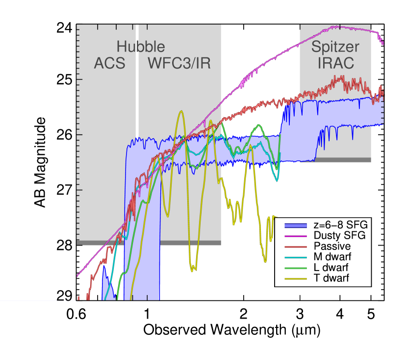
Figure 2: A comparison of the SEDs of star-forming galaxies at high redshift with possible lower-redshift contaminants. The blue shaded region shows model spectra of high-redshift star-forming galaxies (SFGs), with $z=$ 6 as the upper bound, and $z=$ 8 as the lower bound (both models have log(M/M_⊙) $=$ 9.7, an age of 300 Myr, and A_V=0.4). The purple and red lines show a dusty star-forming and a passive galaxy, respectively, both at $z=$ 1.3. Cyan, green and yellow curves denote M, L and T dwarf star empirical near-infrared spectra, taken as the weighted mean of M, L and T dwarf standards from the SpeX Prism Spectral Libraries. The gray shaded regions denote the wavelengths covered by the HST ACS, WFC3/IR and Spitzer/IRAC imaging used in space-based searches for $z>$ 6 galaxies, with the lower bound denoting the magnitude depths at these wavelengths in the CANDELS Deep survey. All contaminants shown would likely satisfy a Lyman break criterion for a $z>$ 6 galaxy, as they would not be detected in typical optical imaging. However, colors at redder observed wavelengths can begin to distinguish between true high-redshift galaxies and low-redshift contaminants, though this can be difficult when working with low signal-to-noise data.

3.5 Contamination

All of the studies discussed above select galaxy candidates, meaning that their derived SEDs are consistent with them lying at a high redshift, but the vast majority have not had their precise redshifts measured with spectroscopy. I will discuss spectroscopic efforts in the following section, but here I discuss the possible sources of contamination. In Figure 2 I show the SEDs of true high redshift galaxies, along with the plausible contaminating sources discussed below.

For continuum-selected galaxies, the most common contaminants are lower-redshift dusty galaxies, lower-redshift passively evolving galaxies, and stars. Low-redshift dusty galaxies can contaminate as they would be observed to have very red colors near the anticipated Lyman break of a true high redshift galaxy. Similarly, a lower-redshift passively evolving galaxy can contaminate if the 4000 Å break is mistaken for the Lyman break (at $z=$ 6 and 8 the redshifts of such contaminants would be $z\sim$ 1.1 and 1.7, respectively). Both types of contamination can happen, as depending on the depth of the imaging used, these contaminants may not be detected in the bluer of the filters used to constrain the Lyman break, and detected in the redder of the filters. However, both types of galaxies should be rejected as they will also have red colors in the filter combination just redward of the desired Lyman break, while true high redshift galaxies are likely bluer. Additionally, extremely dusty galaxies may be detected in mid/far-infrared imaging, which is typically much too shallow to detect true high-redshift galaxies. Photometric redshift analysis techniques typically show that the redder the galaxy, the more probability density shifts from a high redshift solution to a low redshift solution, reflecting the decreased likelihood that the object in question is a truly red high redshift galaxy. For galaxies that are very blue, it is trivial to rule out any possibility of either a dusty or passive low-redshift interloper, but there is usually a non-zero chance of such contamination among the redder galaxies in a given sample. Contamination estimates from such objects are typically low at $<$10% (e.g., Bouwens et al. 2015c; Finkelstein et al. 2015c), though the difficulty of spectroscopically identifying such interlopers makes it difficult to empirically measure this contamination rate.

Stellar contamination is typically handled differently, as many studies search for and remove stellar contaminants after the construction of the initial galaxy sample (e.g., McLure et al. 2006; Bowler et al. 2012, 2014; Bouwens et al. 2015c; Finkelstein et al. 2015c). At $z>$ 6, the colors of M, L and T (brown) dwarf stars can match the colors of candidate galaxies due to the cool surface temperatures of these objects. With HST imaging it can be straightforward to remove the brighter stellar contaminants as the brighter candidate galaxies are all resolved, while stars remain point sources. However, this works less well for fainter galaxies, as near the detection limit it can be difficult to robustly tell whether a given object is resolved. This is not a major problem for HST studies, as at $J>$ 27, the expected surface density of such contaminating stars in the observed fields is low (Finkelstein et al. 2015c; Ryan & Reid 2015).

The more major concern is at intermediate magnitudes, $J=$ 25–26, where the numbers of candidates are small, yet it can be difficult to robustly discern if an object is spatially resolved. To alleviate this issue, for any objects which may be unresolved one can examine whether its observed colors are consistent with any potential contaminating stellar sources. For this to be possible, one needs to ensure that the photometric bands available can robustly delineate between stellar sources and true high-redshift galaxies; as discussed in Finkelstein et al. (2015c), this requires imaging at 1 $\mu$m when working at $z=$ 6–8 (see also Tilvi et al. 2013, for a discussion of the utility of medium bands). Using a combination of object colors and spatial extent, it is likely that space-based studies are relatively free of stellar contamination. This may be more of a problem with ground-based studies, though with excellent seeing even bright $z>$ 6 galaxies can be resolved from the ground (e.g., Bowler et al. 2014). Future surveys must be cognizant of the possibility of stellar contamination, and choose their filter set wisely to enable rejection of such contaminants.

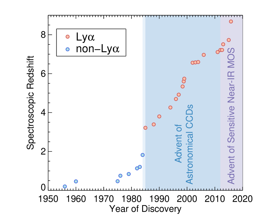
Figure 3: The highest redshift spectroscopically confirmed galaxy plotted versus the year of discovery. There are currently only three galaxies with robust spectroscopic redshifts at $z>$ 7.5: $z=$ 7.51 from Finkelstein et al. (2013), $z=$ 7.73 from Oesch et al. (2015b) and $z=$ 8.68 from Zitrin et al. (2015). Data prior to 1999 were taken from the review of Stern & Spinrad (1999), with the references listed therein. Objects at later times come from Hu et al. (2002); Kodaira et al. (2003); Taniguchi et al. (2005); Iye et al. (2006); Vanzella et al. (2011); Ono et al. (2012); Shibuya et al. (2012); Finkelstein et al. (2013); Oesch et al. (2015b); Zitrin et al. (2015). The shaded regions denote roughly the time when CCDs became widely used, as well as when MOSFIRE (the first highly-sensitive near-infrared multi-object spectrograph) was commissioned on Keck. Major jumps in the most-distant redshift are seen to correspond with these technological advancements.

4 Spectroscopy of $z>$ 6 Galaxies

While photometric selection is estimated to have a relatively low contamination rate, it is imperative to followup a representative fraction of a high-redshift galaxy sample with spectroscopy, to both measure the true redshift distribution, as well as to empirically weed out contaminants. In this section, I discuss recent efforts to spectroscopically confirm the redshifts of galaxies selected to be at $z>$ 6. Figure 3 highlights the redshift of the most distant spectroscopically-confirmed galaxy as a function of the year of discovery.

The most widely used tool for the measurement of spectroscopic redshifts for distant star-forming galaxies is the Ly$\alpha$ emission line, with a rest-frame vacuum wavelength of 1215.67 Å. While at $z<$ 4, confirmation via interstellar medium absorption lines is possible (e.g., Steidel et al. 1999; Vanzella et al. 2009), the faint nature of more distant galaxies renders it nearly impossible to obtain the signal-to-noise necessary on the continuum emission to detect such features. Emission lines are thus necessary, and at $z>$ 3, Ly$\alpha$ shifts into the optical, while strong rest-frame optical lines, such as [O iii] $\lambda\lambda$4959,5007 and H$\alpha\ \lambda$6563 shift into the mid-infrared at $z>$ 4, where we do not presently have sensitive spectroscopic capabilities. Additionally, Ly$\alpha$ has proven to be relatively common amongst star-forming galaxies at $z>$ 3. Examining a sample of $\sim$800 galaxies at $z\sim$ 3, Shapley et al. (2003) found that 25% contained strong Ly$\alpha$ emission (defined as a rest-frame EW $>$ 20 Å), while this fraction increases to $\gtrsim$50% at $z=$ 6 (Stark et al. 2011).

At higher redshifts, Ly$\alpha$ is frequently the only observable feature in an optical (or near-infrared) spectrum of a galaxy. While in principle a single line could be a number of possible features, in practice, the nearby spectral break observed in the photometry (that was used to select a given galaxy as a candidate) implies that any spectral line must be in close proximity to such a break. This leaves Ly$\alpha$ and [O ii] $\lambda\lambda$3726,3729 as the likely possibilities (H$\alpha$ and [O iii], while strong, reside in relatively flat regions of star-forming galaxy continua). While most ground-based spectroscopy is performed at high enough resolution to separate the [O ii] doublet, the relative strength of the two lines can vary depending on the physical conditions in the ISM, thus it is possible only a single line could be observed. True Ly$\alpha$ lines are frequently observed to be asymmetric (e.g., Rhoads et al. 2003), with a sharp cutoff on the blue side and an extended red wing, due to a combination of scattering and absorption within the galaxy (amplified due to outflows), and absorption via the IGM. An observation of a single, asymmetric line is therefore an unambiguous signature of Ly$\alpha$. However, measurement of line asymmetry is only possible with signal-to-noise ratios of $>$10, which is not common amongst such distant objects (e.g., Finkelstein et al. 2013). Lacking an obvious asymmetry, other characteristics need to be considered. For example, for very bright galaxies, the sheer strength of the Lyman break can rule out [O ii] as a possibility, as the 4000 Å break (which would accompany an [O ii] line) is more gradual (see discussion in Finkelstein et al. 2013). For fainter galaxies, with a weaker Lyman break, and no detectable asymmetry, a robust identification of a given line as Ly$\alpha$ is more difficult, and redshift identification should thus be handled with care.

4.1 Spectroscopy at $z=$ 6–6.5

With the advent of ACS on HST, the frontier for spectroscopic confirmations of galaxies moved to $z\sim$ 6. At these redshifts Ly$\alpha$ is still accessible with optical spectrographs and was thus an attractive choice for spectroscopic confirmation. However, the extreme distances means that this line will be extremely faint, thus 8-10m class telescopes were needed to follow them up spectroscopically. One of the first studies to spectroscopically observe Ly$\alpha$ from continuum-selected star-forming galaxies at $z\approx$ 6 was that of Dickinson et al. (2004), who used serendipitous SNe followup ACS grism spectroscopy to detect the Lyman continuum break from one galaxy, following it up with LRIS on Keck to discover Ly$\alpha$ emission at $z=$ 5.8. At that same time Stanway et al. (2004) used the GMOS optical spectrograph on the Gemini 8.2m telescope to measure the redshifts to three galaxies discovered in the ACS imaging of the HUDF, at $z=$ 5.8–5.9 (one of these, originally published by Bunker et al. (2003), is bright enough to spectroscopically detect the Lyman break). Stanway et al. (2007) continued this survey, confirming the redshifts to two additional galaxies, at $z=$ 5.9–6.1. Dow-Hygelund et al. (2007) added another six redshifts via Ly$\alpha$ at $z=$ 5.5–6.1. In a series of papers by Vanzella et al., a larger sample of confirmed $z\approx$ 6 galaxies was obtained with the FORS2 spectrograph on the 8.2m VLT, culminating in the spectroscopic confirmation of a total of 32 $z\sim$ 6 galaxies (Vanzella et al. 2006, 2008, 2009).

Another effort for $z\sim$ 6 spectroscopic followup comes from Stark et al. (2010, 2011), who used the DEIMOS optical spectrograph on Keck to spectroscopically observe continuum selected star-forming galaxies at 4 $<z<$ 6. In particular, Stark et al. (2011) obtained a very deep 12.5 hr single mask observation with DEIMOS, measuring the redshifts for 11 galaxies at 5.7 $<z<$ 6.0 via Ly$\alpha$ emission. Stark et al. (2011) examined the fraction of galaxies with strong (here defined as EW $>$ 25 Å) Ly$\alpha$ emission, finding that for fainter galaxies (M${}_{UV}>-$20.25) it rises from $\sim$35% at $z=$ 4, to $\sim$55% at $z\sim$ 6 (for brighter galaxies, the fraction rises from $\sim$10% at $z=$ 4 to $\sim$20% at $z=$ 6). These results imply that galaxies at higher redshifts have a higher escape fraction of Ly$\alpha$ photons, potentially due to reduced dust attenuation. In addition to measuring the redshifts of many galaxies at $z\sim$ 6, the rising fraction of galaxies with detectable Ly$\alpha$ emission with increasing redshift implied that Ly$\alpha$ should continue to be a very useful tool at $z>$ 6.5.

HST provides an alternative to ground-based spectroscopy, as ACS has grism spectroscopic capabilities. In this mode, one obtains very low resolution spectra for every object in the camera’s field. The main advantage is in the multiplexing. The primary disadvantage is the contamination from overlapping sources, though this can be mitigated by splitting the observations over multiple roll angles. Due to the very low resolution (the G800L grism on ACS has R $\sim$ 100), only very strong emission lines can be detected. However, the very low sky background affords this mode much greater continuum sensitivity, particularly when searching for galaxies at $z>$ 6, where the night sky emission makes continuum detections from the ground problematic. There have thus been a number of HST surveys seeking to confirm galaxy redshifts via a detection of the Lyman continuum break. This provides somewhat less precision than an emission line detection, but if the sharpness of the break can be measured, one can confirm that the break seen in photometry is indeed the Lyman break (which is sharp, in contrast to the 4000 Å break which is more extended in wavelength; see Figure 2).

The GRAPES survey (PI Malhotra) obtained deep ACS grism observations over the HUDF. Malhotra et al. (2005) presented the spectroscopic confirmation of 22 galaxies at 5.5 $<z<$ 6.7 from this survey, detecting the continuum break from galaxies as faint as $z_{\mathrm{AB}}\sim$ 27.5. The PEARS survey (PI Malhotra) extended these observations to cover eight additional pointings in the GOODS fields, culminating in the spectroscopic detection of a Lyman break at $z=$ 6.6 (with $z_{\mathrm{AB}}=$ 26.1). Ground-based followup with the Keck 10m telescope showed a Ly$\alpha$ emission line at $z=$ 6.57 for this galaxy, confirming its high-redshift nature (Rhoads et al. 2013). The WFC3/IR camera also has grism capability, and there are have been efforts (though none succesful at this time; e.g., Pirzkal et al. 2015) to confirm redshifts at $z>$ 7 with HST. The in-progress FIGS (PI Malhotra), CLEAR (PI Papovich) and GLASS (PI Treu; Schmidt et al. 2016) surveys may change this, as the very deep spectroscopy should detect Ly$\alpha$ emission or possibly continuum breaks for galaxies out to $z\sim$ 8.

4.2 Pushing to $z>$ 6.5: A deficit of Ly$\alpha$ emission?

As the first $z\sim$ 7 galaxy samples began to be compiled with the initial WFC3/IR surveys and ground-based surveys, confirmation via Ly$\alpha$ was an obvious next step. However, this proved more difficult than thought. One of the first hints that not all was as expected came from Fontana et al. (2010), who observed seven candidate $z>$ 6.5 galaxies with FORS2 on the VLT. Given the expected Ly$\alpha$ EW distribution and the magnitudes of their targeted sample, they expected to detect three Ly$\alpha$ emission lines at $\geq$10$\sigma$ significance, yet they found none (Ly$\alpha$ emission from one galaxy was detected at 7$\sigma$ significance at $z=$ 6.972). Progress was still made, as Pentericci et al. (2011) and Vanzella et al. (2011) each reported the confirmation of two galaxies via Ly$\alpha$, at $z\sim$ 6.7 in the former, and $z=$ 7.0-7.1 in the latter. Yet, as discussed in Pentericci et al. (2011), the fraction of confirmed galaxies was only 25%, much less than the $\gtrsim$50% predicted by Stark et al. (2011).

Table 1: Spectroscopically Confirmed Galaxies at $z>$ 7

ID	Ly$\alpha$ Redshift	MUV	Rest-Frame Ly$\alpha$ EW (Å)	Reference
BDF-521	7.008	$-$20.6	64${}^{+10}_{-9}$	Vanzella et al. (2011)
A1703-zD6	7.045	$-$19.4	65 $\pm$ 12	Schenker et al. (2012)
BDF-3299	7.109	$-$20.6	50${}^{+11}_{-8}$	Vanzella et al. (2011)
GN 108036	7.213	$-$21.8	33	Ono et al. (2012)
SXDF-NB1006-2	7.215	$-$22.4	15${}^{+\inf}_{-5}$	Shibuya et al. (2012)
z8_GND_5296	7.508	$-$21.2	8 $\pm$ 1	Finkelstein et al. (2013)
z7_GSD_3811	7.664	$-$21.2	16${}^{+6}_{-4}$	Song et al. (2016)
EGS-zs8-1	7.730	$-$22.0	21 $\pm$ 4	Oesch et al. (2015b)
EGSY8p7	8.683	$-$22.0	28${}^{+14}_{-11}$	Zitrin et al. (2015)
ULAS J1120+0641	7.085	—	—	Mortlock et al. (2011)
GRB 090423	8.3	—	—	Tanvir et al. (2009)

The upper portion of the table contains published redshifts based on significantly detected ($>$5$\sigma$) Ly$\alpha$ emission at $z>$ 7. We include published uncertainties on the equivalent width when available. Not listed are two additional sources which fall in the 4–5$\sigma$ significance range, from Schenker et al. (2014) at $z=$ 7.62, and Roberts-Borsani et al. (2015) at $z=$ 7.47. The bottom portion contains the highest redshift spectroscopically confirmed quasar (via several emission lines, including Ly$\alpha$), and gamma-ray burst (via spectroscopic observations of the Lyman break), respectively.

Observations of galaxies in this epoch were also performed by Ono et al. (2012) and Schenker et al. (2012), confirming Ly$\alpha$-based redshifts at $z=$ 7-7.2, yet still finding less galaxies that would be the case if the Ly$\alpha$ EW distribution was unchanged from $z=$ 6. Pentericci et al. (2014) recently published an extended sample, reporting Ly$\alpha$ emission from only 12 of 68 targeted sources at $z\gtrsim$ 6.5. After accounting for the depth of observations and accurate modeling of night sky emission, Pentericci et al. (2014) found the fraction of faint galaxies with Ly$\alpha$ EW $>$25 Å to be only $\sim$30%. This deficit is unlikely to be due to significant contamination, as Pentericci et al. (2011) showed a much higher fraction of detectable Ly$\alpha$ emission from galaxies at $z\sim$ 6 selected in a similar way.

Part of these difficulties may be technological in nature, as at $z>$ 6.5, these observations were working at the extreme red end of optical spectrographs, where the sensitivity begins to be dramatically reduced. Until recently, similarly efficient multi-object spectrographs operating in the near-infrared were not available. This changed with the installation of MOSFIRE on the Keck I telescope in 2012. Finkelstein et al. (2013) used MOSFIRE to observe $>$40 galaxies at $z=$ 7–8 from the CANDELS survey in GOODS-N, obtaining very deep 5 hr integrations over two configurations (of $\sim$ 20 galaxies each). A single emission line was detected, which was found to be Ly$\alpha$ from a galaxy at $z=$ 7.51, the most distant spectroscopic detection of Ly$\alpha$ at that time. Accounting for incompleteness due to wavelength coverage and spectroscopic depth, Finkelstein et al. (2013) found that they should have detected Ly$\alpha$ from $\sim$six galaxies, finding that the Ly$\alpha$ “deficit” continues well beyond $z=$ 7. Other observations have been performed with MOSFIRE, yet most have only achieved relatively short exposure times, resulting in primarily non-detections (e.g., Treu et al. 2013; Schenker et al. 2014). Recently, two new record holders for the most distant spectroscopically confirmed galaxy at the time of this writing have been found, at $z=$ 7.73 by Oesch et al. (2015b) and at $z=$ 8.68 by Zitrin et al. (2015), both detected with MOSFIRE. Interestingly, the four highest redshift galaxies known, at $z=$ 7.5–8.7 (including a recent detection at $z=$ 7.66 by Song et al. 2016), all appear to have very low Ly$\alpha$ EWs (of $<$ 30 Å, respectively) and thus are not similar to the much higher EW sources frequently seen at $z\lesssim$ 6. In Table 1 I summarize the currently known spectroscopically-confirmed galaxies at $z>$ 7. Of note here are again the relatively low EWs, especially at $z>$ 7.2, as well as the bright UV magnitudes of the confirmed sources.

While there have been some notable successes in the search for Ly$\alpha$ emission at $z>$ 7, in general all studies report Ly$\alpha$ detections from fewer objects than expected, as well as weak Ly$\alpha$ emission from any detected objects. It thus appears that something, either in the physical conditions within the galaxies, or in the universe around them, is causing either less Ly$\alpha$ photons to be produced, or preventing most of them from making their way to our telescopes. I will discuss physical possibilities for this apparent lack of strong Ly$\alpha$ emission in §7.1.3.

4.3 Alternatives to Ly$\alpha$

Given the apparent difficulties with detecting Ly$\alpha$ at $z>$ 6.5, it is prudent to examine whether other emission lines may be useful as spectroscopic tracers. While photometric colors imply these galaxies likely have strong rest-frame optical emission (e.g., Finkelstein et al. 2013; Smit et al. 2014; Oesch et al. 2015b), spectroscopic observations of for example [O iii] requires JWST. However, there may be weaker rest-frame UV emission lines that can be observed. Erb et al. (2010) published a spectrum of a blue, low-mass star-forming galaxy at $z\sim$ 2 (called BX418) which possessed physical characteristics similar to typical galaxies at $z>$ 6. Among the interesting features in the spectrum of this object was detectable emission lines of He ii $\lambda$1640 and C iii] $\lambda\lambda$1907,1909. Stark et al. (2014) obtained deep optical spectroscopy of 17 similarly low-mass $z\sim$ 2 galaxies, finding nearly ubiquitous detections of C iii]. The strength of this emission was on average 10% that of Ly$\alpha$. However, at $z>$ 6.5, most of the Ly$\alpha$ is being attenuated (or scattered); for example, the strength of Ly$\alpha$ at $z=$ 7.51 observed by Finkelstein et al. (2013) was only $\sim$10% of that expected from the stellar population of the galaxy. Thus, exposures deep enough to detect Ly$\alpha$ may also detect C iii] at very high redshift. Stark et al. (2015) searched for C iii] from two galaxies with known Ly$\alpha$ redshifts at $z>$ 6, obtaining tenuous $\sim$3$\sigma$ detections of C iii] at $z=$ 6.029 and $z=$ 7.213. Part of the difficulty at higher redshift is because the C iii] doublet becomes resolved (splitting the line flux over more pixels), yet these possible detections imply this may be a promising line for future study. Some progress may be made with MOSFIRE on Keck, though multi-object spectrographs on the next generation of telescopes, such as the 25m Giant Magellan Telescope or the Thirty Meter Telescope, will have the capability to probe these alternative UV emission features to very faint levels, probing the redshifts of galaxies out to $z>$ 10.

5 The Evolution of the Rest-Frame UV Luminosity Function

One of the most straightforward, and also useful, measures we can make of distant galaxies is the measurement of the rest-frame UV luminosity function. In this section, I will discuss the usefulness of this observation and recent measurements in the literature. I will also derive a “reference” luminosity function, as a Schechter fit to all recent data points from the literature.

5.1 The Significance of the UV Luminosity Function

Distribution functions are an immensely useful quantity to measure as they are relatively straightforward to compute in both observations and theory, and thus provide a direct means to compare the two. Distribution functions of galaxy luminosities, stellar masses, and even velocity dispersions have been measured at a variety of redshifts, leading to detailed insight into the physical processes inherent in galaxy evolution. At $z>$ 6, however, we are limited in what we can measure. The rest-frame UV is the wavelength regime which can be observed very deeply from the ground and with HST, thus the galaxy rest-frame UV luminosity function is the best-studied distribution function at such redshifts. While stellar mass functions are also useful (and will be discussed in the next section), it is much more direct to correct the UV luminosity function for incompleteness, as the luminosity is a direct observable, while the stellar mass is a derived quantity. There is a downside to the UV luminosity, in that it is highly susceptible to dust attenuation, thus to compare observations to theory simulations must add dust attenuation, or observations must attempt to correct for this attenuation.

Observations of luminosity functions at lower redshifts have shown that it typically follows a characteristic shape with a power-law slope at the faint end and an exponential decline at the bright-end, transitioning at a characteristic magnitude or luminosity typically referred to as the “knee” of the luminosity function. Parameterized by Schechter (1976), the “Schechter function” requires three parameters to describe this shape: the characteristic magnitude or luminosity at the knee (M^∗ or L^∗), the power-law slope at the faint end ($\alpha$), and the characteristic number density ($\phi^{\ast}$) which is a normalization factor which defines the overal number density of galaxies. Schechter function parameterizations for luminosity and magnitudes are given in Equations 1 and 2, respectively (in units of number per magnitude or luminosity bin, per volume).

$$\phi(L)=\phi^{\ast}\left(\frac{L}{L^{\ast}}\right)^{\alpha}\mathrm{exp}\left(-\frac{L}{L^{\ast}}\right)$$ (1)

$$\begin{split}\phi(M)=0.4~{}\mathrm{ln}~{}(10)\!~{}\phi^{\ast}\!~{}10^{-0.4(M-M^{\ast})(\alpha+1)}\\ e^{-10^{-0.4(M-M^{\ast})}}\end{split}$$ (2)

A comparison between the shape of the luminosity function and that of the underlying halo mass function can provide insight into the mechanisms driving galaxy evolution. A simple toy model may assume that the shape of the luminosity function is similar to that of the halo mass function, scaling for some constant baryon conversion efficiency. However, as shown in Figure 4, this is not the case. In this figure, I show the $z=$ 7 luminosity function from Finkelstein et al. (2015c), along with the halo mass function at $z=$ 7 from the Bolshoi $\Lambda$CDM simulation (Klypin et al. 2011), measured by Behroozi et al. (2013b). I place the luminosity function on this figure by converting from luminosity to stellar mass via the liner relation derived by Song et al. (2015), and scaling vertically such that the two distribution functions touch at the knee. Assuming in this case a ratio of halo mass to stellar mass of 80, the number densities match at log (M_halo/M_⊙) $\sim$ 11.5 (approximately the halo mass of a L^∗ galaxy at this redshift; Finkelstein et al. 2015b), yet the number of both more and less massive halos is higher than that of galaxies. To phrase this another way, the conversion of gas into stars in galaxies in both more and less massive halos is less efficient.

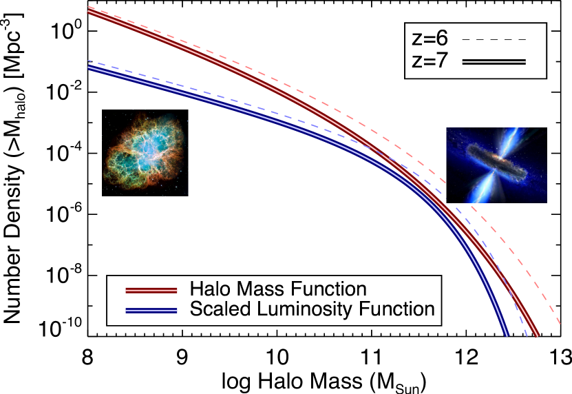
Figure 4: The cumulative halo mass function from the Bolshoi simulations at $z=$ 6 and 7, shown in red. In blue, I show the cumulative luminosity functions from Finkelstein et al. (2015c), using the relation between stellar mass and UV absolute magnitude from Song et al. (2015), and scaling by a stellar mass-to-halo mass ratio such that the $z=$ 7 functions match at the knee. Even after this scaling, there is still a discrepancy, which is commonly attributed to feedback due to supernovae at the faint end, and AGN feedback at the bright end (image of the Crab Nebula from Loll et al. 2013).

Such differences have been observed at all redshifts where robust luminosity functions exist, and a number of physical mechanisms have been proposed for this observation. One mechanism that is currently actively debated is that of feedback. Models which invoke feedback, typically due to supernovae (primarily at the faint-end), stellar radiative feedback, and (primarily at the bright end) accreting supermassive black hole/active galactic nucleus (AGN) feedback (see discussion of these processes in the review of Somerville & Davé 2015, and references therein) can more successfully match observations than those which do not include such effects, in which case too many stars are frequently formed. This feedback can heat and/or expel gas from galaxies, effectively reducing, or even quenching further star-formation. Such feedback can explain a variety of observations. For example, the mass-metallicity relation observed at lower redshift (e.g., Tremonti et al. 2004; Erb et al. 2006) can be explained by supernova-driven winds preferentially removing metals from lower-mass galaxies, while the increased potentials from higher mass galaxies allows retention of these metals; (e.g., Davé et al. 2011).

Given that these physical processes affect the shape of the luminosity function, studying the evolution of this shape with redshift can therefore provide information on the evolution of these processes. Observations have shown that the abundance of bright quasars decreases steeply at $z>$ 3 (e.g., Richards et al. 2006). Although bright quasars do exist at $z>$ 6 (Fan et al. 2006), they are exceedingly rare. Thus, if AGN feedback was the primary factor regulating the bright end of the luminosity function, one may expect a decrease in the difference between the luminosity function and the halo mass function at high redshift. Likewise, if supernova feedback became less efficient at higher redshift, one would expect the faint-end slope to steepen at high redshift, approaching that of the halo mass function ($\alpha\sim-$2). In practice, this is more complicated, as other effects are in play, such as luminosity-differential dust attenuation (e.g., Bouwens et al. 2014), and perhaps a changing star-formation efficiency (e.g., Finkelstein et al. 2015b). Nonetheless, the shape of the luminosity function is one of the key probes that we can now measure which can begin to constrain these processes.

The integral of the rest-frame UV luminosity function is also a physically constraining quantity. As the UV luminosity probes recent star-formation (on timescales of $\sim$100 Myr; Kennicutt 1998), the integral of the UV luminosity function, corrected for dust, measures the cosmic star-formation rate density in units of solar masses per year per unit volume. One can measure this quantity as a function of redshift, and such a figure shows that from the present day this quantity rises steeply into the past (e.g., Lilly et al. 1996; Schiminovich et al. 2005), peaking at $z\sim$ 2–3 (e.g., Reddy & Steidel 2009), and declining at $z>$ 3 (e.g., Madau et al. 1996; Steidel et al. 1999; Bouwens et al. 2007). A recent review of this topic can be found in Madau & Dickinson (2014). The extension of the cosmic SFR density to $z>$ 6 can provide detailed constraints on the buildup of galaxies at early times. If it continues in a smooth trend, as observed from $z\sim$ 3 to 6, it implies a smooth buildup of galaxies from very early times. Alternatively, if the SFR density exhibits a steep dropoff at some redshift, it may imply that we have reached the epoch of initial galaxy formation.

Finally, another use of the integral of the rest-frame UV luminosity function is as a constraint on reionization. Galaxies are the leading candidate for the bulk of the necessary ionizing photons for reionization. By assuming a (stellar-population dependent) conversion between non-ionizing and ionizing UV luminosity, one can convert the integral of the UV luminosity function (the specific luminosity density, in units of erg s^-1 Hz^-1 Mpc^-3) to an ionizing emissivity, in units of photons s^-1 Mpc^-3. This can then be compared to models of the needed ionizing emissivity to reionize the IGM, to assess the contribution of galaxies to reionization. As shown over a decade ago, galaxies much fainter than the detection limit of HST are likely needed to complete reionization (e.g., Bunker et al. 2004; Yan & Windhorst 2004). Thus, measuring an accurate faint-end slope is crucial to allow a robust measurement of the total UV luminosity density, and thus the total ionizing emissivity. I will cover this issue in §7.

5.2 Observations at $z=$ 6–10

In §3.1 and 3.2, I covered recent surveys for star-forming galaxies at $z\geq$ 6. Here I will discuss the measurements of the rest-frame UV luminosity function from these surveys. A number of recent papers have studied this quantity at $z=$ 6 (Bouwens et al. 2007; McLure et al. 2009; Willott et al. 2013; Bouwens et al. 2015c; Finkelstein et al. 2015c; Bowler et al. 2015; Atek et al. 2015; Livermore et al. 2016), $z=$ 7 (Ouchi et al. 2009; Castellano et al. 2010; Bouwens et al. 2011b; Tilvi et al. 2013; McLure et al. 2013; Schenker et al. 2013; Bowler et al. 2014; Bouwens et al. 2015c; Finkelstein et al. 2015c; Atek et al. 2015; Livermore et al. 2016), $z=$ 8 (Bouwens et al. 2011b; McLure et al. 2013; Schenker et al. 2013; Schmidt et al. 2014; Bouwens et al. 2015c; Finkelstein et al. 2015c; Atek et al. 2015; Livermore et al. 2016), $z=$ 9 (McLure et al. 2013; Oesch et al. 2013, 2014; McLeod et al. 2015; Bouwens et al. 2015b; Ishigaki et al. 2015) and $z=$ 10 (Oesch et al. 2015a; Bouwens et al. 2015c, b). In the interest of presenting constraints from the most recent studies in a concise manner, I will focus on the studies of Bowler et al. (2014, 2015), Finkelstein et al. (2015c), Bouwens et al. (2015c) at $z=$ 6–8, and Bouwens et al. (2015b) and McLeod et al. (2015) at $z=$ 9–10.

At $z=$ 6–8, Finkelstein et al. (2015c) and Bouwens et al. (2015c) used data from the CANDELS and HUDF surveys, while Bowler et al. (2014, 2015) used ground-based imaging from the UltraVISTA and UKIDSS UDS surveys to discover brighter galaxies. Finkelstein et al. (2015c) used only data from the CANDELS GOODS-N and GOODS-S fields, which have deep HST imaging in seven optical and near-infrared filters, versus only four filters in the other three fields. Specifically, only the CANDELS GOODS fields have deep space-based $Y$-band imaging, which is necessary for robust removal of stellar contaminants (Finkelstein et al. 2015c). Bouwens et al. (2015c) used all five CANDELS fields, making use of ground-based optical and $Y$-band imaging to fill in the missing wavelengths from HST. Both studies use the HUDF and associated parallels, while Finkelstein et al. (2015c) also used the parallels from the first year of the Hubble Frontier Fields program, and Bouwens et al. (2015c) used the BoRG/HIPPIES pure parallel program data (Schmidt et al. 2014).

In spite of different data reduction schemes, selection techniques, data used, and completeness simulations, the results of Finkelstein et al. (2015c) and Bouwens et al. (2015c) are broadly similar (Figure 6). Both studies find a characteristic magnitude M^∗ which is constant or only weakly evolving from $z=$ 6–8, and both find a significantly evolving faint-end slope (to steeper values at higher redshift), and characteristic number density $\phi^{\ast}$ (to lower values at higher redshift). This is a change from initial studies at $z>$ 6 (most probing smaller volumes), which found that M^∗ significantly evolved to fainter values from $z=$ 4 to 8, with less evolution in $\phi^{\ast}$ (e.g., Bouwens et al. 2007, 2011b; McLure et al. 2013). The faint-end slope $\alpha$ now appears to match (or even exceed) the value from the halo mass function ($\alpha\sim-$2) at the highest redshifts ($\alpha<-$2 can be possible due to effects of baryonic physics). The primary difference between these studies appears to be in the normalization, as the Bouwens et al. (2015c) data points are systematically slightly higher/brighter than those of Finkelstein et al. (2015c), which can be attributed to differences in the assumed cosmology ($\sim$5%), aperture corrections utilized to calculate the total fluxes in the photometry, and differences in contamination.

As Bowler et al. (2014, 2015) used ground-based data to probe larger volumes, they were thus sensitive to brighter galaxies than either Finkelstein et al. (2015c) or Bouwens et al. (2015c). Broadly speaking their results are consistent with the HST-based studies where there is overlap. However, there does seem to be a modest tension, in that the Bowler et al. (2014, 2015) ground-based results exhibit slightly lower number densities than those from either of the space-based studies, though the tension only exceeds 1$\sigma$ significance at the faintest ground-based magnitude (M${}_{\mathrm{UV}}=-$21.5). This is true compared to both HST studies at $z=$ 7, while Bowler et al. (2015) and Finkelstein et al. (2015c) are in agreement at $z=$ 6. To fit a Schechter function, Bowler et al. (2015) combine their data with data at fainter luminosities from Bouwens et al. (2007) at $z=$ 6, while Bowler et al. (2014) combine with fainter data from McLure et al. (2013) at $z=$ 7. The combination of the deeper HST imaging with their much larger volumes allows the ground-based studies to perhaps place tighter constraints on M^∗. They do find more significant evolution in M^∗ than that found by Finkelstein et al. (2015c) or Bouwens et al. (2015c), with M${}^{\ast}_{z=7}=-$20.56 $\pm$ 0.17, compared to $-$21.03${}^{+0.37}_{-0.50}$ from Finkelstein et al. (2015c) and $-$20.87 $\pm$ 0.26 from Bouwens et al. (2015c). Given these uncertainties, some evolution in M^∗ towards fainter luminosities at higher redshift is certainly plausible (including the modest $dM/dz=$ 0.2 proposed by Bowler et al.), and there appears no strong disagreement between these complementary studies. The data points from these three studies, as well as a number of other recent works, are shown in Figure 5, and the fiducial Schechter function parameters are shown in Figure 6.

Given the wide dynamic range now probed in luminosity, each of the aforementioned studies understandably pay careful attention to the shape of the luminosity function. Specifically, they investigate whether a Schechter function shape is required by the data, or whether another function, such as a double power law (where the bright-end exponential cutoff is replaced by a second power law), or even a single power law (where the exponential cutoff disappears altogether) is demanded. Finkelstein et al. (2015c) considered all three functions. While they found significant evidence that a Schechter function was required at $z=$ 6 and 7, at $z=$ 8 the luminosity function was equally well fit by a single power law as by a Schechter function. This is intriguing, as this is exactly the signature one might expect were AGN feedback to stop suppressing the bright end (changing dust attenuation is likely not a dominant factor, as bright galaxies at $z=$ 6–8 have similar levels of attenuation; Finkelstein et al. 2012b, e.g.,; Bouwens et al. 2014, e.g.,; Finkelstein et al. 2015b, e.g.,). Bouwens et al. (2015c) found a similar result, claiming that there was no overwhelming evidence to support a departure from a Schechter function, but that the available data at $z>$ 6 made it difficult to constrain the exact functional form.

While Bowler et al. (2015) reach a similar conclusion at $z=$ 6, in that either a double power law or a Schechter functional form could explain the bright end shape, at $z=$ 7 Bowler et al. (2014) find significant evidence that a double power law is a better fit than Schechter. With this result, they find that the shape of the bright end closely matches that of the underlying halo mass function, implying little quenching in bright galaxies at $z=$ 7. Bouwens et al. (2015c) discuss this difference in conclusions, and attribute it to the differences in the measured number density at $M=-$21.5; the higher number densities found by the HST studies allow a Schechter function to be fit equally well. In any case, at $z>$ 6, there no longer remains overwhelming evidence to support a Schechter function parameterization. To robustly constrain the shape of the luminosity function requires further data, in particular in the overlap range between the ground-based and HST studies.

At higher redshifts of $z=$ 9–10, the data do not currently permit such detailed investigations into the shape of the luminosity function. However, we have begun to gain our first glimpse into the evolution of the Schechter parameters to the highest redshifts (if, in fact, this function ultimately does describe the shape of the luminosity functions). Studies of galaxies at these redshifts are difficult with the data used in the above studies, as at these redshifts the Lyman break passes through the HST/WFC3 F125W filter, rendering most objects only detectable in the F160W filter in the CANDELS fields. Nonetheless, several groups have attempted to select F125W-dropout galaxies, with some using Spitzer/IRAC data as a potential secondary detection band (e.g., Oesch et al. 2014). Additionally, recent surveys have started adding observations in the HST/WFC3 F140W filter, which should show a detection for true $z\approx$ 9 galaxies, though galaxies at $z>$ 10 may still have most of their flux attenuated by the IGM in that band.

McLeod et al. (2015) probed the faint-end at $z\sim$ 9 using data from the first year of the Hubble Frontier Fields (though they explicitly do not include regions with high magnifications), which contains F140W imaging, allowing for robust two-band detections. They found 12 new $z\sim$ 9 galaxy candidates in these data, which they combined with previously discovered $z\sim$ 9 candidates in the HUDF from McLure et al. (2013) to constrain the luminosity function. They do not fit all Schechter parameters, choosing to leave the faint-end slope fixed to $\alpha=-$2.02, and explore possible values of the characteristic magnitude and normalization under the scenarios of pure density or pure luminosity evolution. They find only modest evolution from $z=$ 8, consistent with a continued smooth decline in the UV luminosity density. Bouwens et al. (2015b) recently searched the CANDELS fields for bright $z\sim$ 9 and 10 galaxies, finding nine $z\sim$ 9 galaxies, and five $z\sim$ 10 galaxies (all with $H<$ 27). They do not attempt to derive Schechter function parameters, rather they use the redshift evolution of said parameters from Bouwens et al. (2015c) to show that it is consistent with their updated results at the bright end, as well as results from the literature at the faint end. They however conclude that the UV luminosity density at $z\sim$ 9 and 10 is $\sim$2$\times$ lower than would be expected when extrapolating the observed trend from $z\sim$ 4–8.

These studies highlight the remarkable capability of the modestly-sized Hubble to study galaxies to within 500 Myr after the Big Bang. However, the sizable uncertainties remaining, especially at $z>$ 8, lead to fundamental disagreements about the evolution of the UV luminosity density (§5.4) which will likely not be resolved until the first datasets come in from JWST.

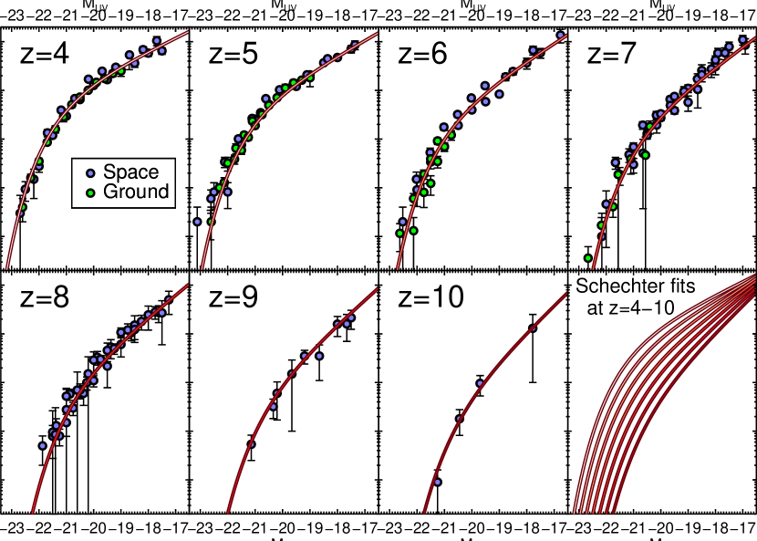
Figure 5: A compilation of luminosity function data from the literature. Data from space-based surveys are shown in blue, and ground-based surveys in green. In each panel, I show the reference Schechter function fit (§5.3) to all available data points as the red curves. The lower-right panel overplots the fiducial Schechter functions together at all five redshifts. These Schechter function values and associated uncertainties are given in Table 2. The studies used in the fitting are: Bouwens et al. (2015c) at $z=$ 4–10; Finkelstein et al. (2015c) at $z=$ 4–8; van der Burg et al. (2010) at $z=$ 4–5; McLure et al. (2009) at $z=$ 5–6; McLure et al. (2013) at $z=$ 7–9; Schenker et al. (2013) at $z=$ 7–8; Bouwens et al. (2015b) at $z=$ 9–10; Bowler et al. (2015) at $z=$ 6; Castellano et al. (2010), Tilvi et al. (2013) and Bowler et al. (2014) at $z=$ 7; Schmidt et al. (2014) at $z=$ 8; Oesch et al. (2013) and McLeod et al. (2015) at $z=$ 9; and Oesch et al. (2014) and McLeod et al. (2016) at $z=$ 10.

5.3 A Reference Luminosity Function

As discussed at the beginning of the previous subsection, many groups have published measurements of rest-frame UV luminosity functions at $z\geq$ 6. There are a variety of datasets used, both deep space-based, and relatively shallow ground-based, thus one study alone may not have the dynamic range to fully constrain the full luminosity function. As a perhaps crude, yet illustrative attempt to shed light on the evolution of this useful tool, in this subsection I combine published results from a number of studies in an attempt to derive a set of “reference” rest-frame UV luminosity functions at $z=$ 4–10. I use the data from all studies listed in the first paragraph of §5.2 where the luminosity function data was available, with the exception of the $z=$ 6 results from Willott et al. (2013) as Bowler et al. (2015) found that the Willott et al. sample did not include many true $z\sim$ 6 galaxies, possibly due to the shallowness of the earlier data. Likewise, I do not include the $z=$ 7 results from Ouchi et al. (2009), as they applied a very high contamination correction of 50%; see discussion in Appendix F.3 of Bouwens et al. (2015c). I also do not include the data from Bouwens et al. (2007, 2011b), as they are superseded by Bouwens et al. (2015c). Finally, I do not include the recent lensed luminosity functions of Ishigaki et al. (2015), Atek et al. (2015), or Livermore et al. (2016) due to the likely strong presence of Eddington bias (see discussion in Livermore et al. 2016).

I acknowledge that many of these studies use similar datasets in the same survey fields, thus the same galaxies may contribute to multiple data points, and this analysis does not include possible systematic effects which could broaden the error budget. However, even studies which utilize the same surveys use a wide range of data reduction, photometry, and sample selection techniques which can and does result in differences in the measured number densities at a given magnitude (Figure 5). The results of this analysis are illustrative of the constraints possible when marginalizing over these differences, as well as when combining ground with space-based datasets. However, I do acknowledge that the faintest data points used typically all come from the same field: the HUDF. Therefore, during the MCMC analysis (described below), in magnitudes bins at $-$18 or fainter each step of the MCMC chain randomly chooses one data point per magnitude bin. This should suppress any “artificial” damping of the uncertainties on the faint-end slope, as during each step we use only a single measurement from the HUDF per magnitude bin.

From each of the studies used, I extracted the measured, completeness corrected, number densities (and associated uncertainties) as a function of UV absolute magnitude, shown in Figure 5. I then calculated the likelihood that the data were represented by a given Schechter function via a Markov Chain Monte Carlo (MCMC) algorithm. I used an IDL implementation (R. Ryan, private communication) of the Python $\tt{Emcee}$ package (Foreman-Mackey et al. 2013), which utilizes an affine-invariant ensemble sampler to sample the parameter space. However, rather than fitting a Schechter function to each redshift independently, I made the assumption that the Schechter function parameters linearly vary with redshift. This is an assumption often assumed in the literature, though typically after the fact (e.g., Bouwens et al. 2015c; Finkelstein et al. 2015c). The advantage of this method is that it allows the data from all redshifts to be fit simultaneously, solving for the posterior distribution of the coefficients of the linear function which describes $M^{\ast}(z)$, $\phi^{\ast}(z)$ and $\alpha(z)$. In effect, this replaces 21 parameters (the three Schechter parameters at seven redshifts) with six parameters: the slope and intercept of the three redshift-dependent Schechter parameter trends. An additional advantage is that this method allows convergence of the chain even at $z=$ 9 and 10, where there are few datapoints. Without the assumption of linear evolution, a prior would have to be placed on the individual Schechter parameters at these highest redshifts to obtain a result.

Figure 6: The derived evolution of the three Schechter function parameters with redshift, derived by fitting all redshifts simultaneously. The shaded blue regions denote the 68% confidence range of the linear evolution of these parameters with redshift, while the circles denote the reference value at a given redshift. Evolution with increasing redshift in $M^{\ast}$ (to fainter values), $\alpha$ (to steeper values) and $\phi^{\ast}$ (to lower values) is detected at $>$10$\sigma$ significance.

I ran the MCMC algorithm for 10⁶ total steps, and checked each parameter for convergence using the Geweke diagnostic, which compares the average and the variance of the first 10% to the last half of the steps (Geweke 1992). For each of the six parameters of the fit, I calculated the median value and the 68% confidence range from the median and central 68% range of the posterior distribution, respectively. The results are:

$$M^{\ast}(z) =-20.79_{-0.04}^{+0.05}+0.13_{-0.01}^{+0.01}~{}(z-6)$$

$$\alpha(z) =~{}\!\!-1.91_{-0.03}^{+0.04}-0.11_{-0.01}^{+0.01}~{}(z-6)$$

$$log~{}\phi^{\ast}(z) =~{}\!\!-3.37_{-0.04}^{+0.05}-0.19_{-0.01}^{+0.01}~{}(z-6)$$

The fiducial Schechter functions from this exercise derived by evaluating the above equations at a given redshift are shown alongside the data points in Figure 5 and the values are tabulated with their uncertainties in Table 2. In the lower-righthand panel of Figure 5, I show the fiducial Schechter functions from this analysis at $z=$ 4–10 together, highlighting a relatively smooth decline from $z=$ 4 to 10. In Figure 6 I show the redshift-dependent Schechter parameter evolution with the median values at each redshift, along with the results of a variety of studies listed above. The reference results are for the most part consistent with results in the literature within the uncertainties (with the exception of M^∗ at $z=$ 4, which is brighter than the value found by Bouwens et al. (2015c) and Finkelstein et al. (2015c)).

Table 2: Median Schechter Parameters to Compilation of Literature Data

Redshift	M∗	$\alpha$	$log\phi^{\ast}$
4	$-$21.05${}^{+0.05}_{-0.06}$	$-$1.69${}^{+0.03}_{-0.04}$	$-$2.99${}^{+0.04}_{-0.04}$
5	$-$20.92${}^{+0.05}_{-0.05}$	$-$1.80${}^{+0.04}_{-0.04}$	$-$3.18${}^{+0.04}_{-0.04}$
6	$-$20.79${}^{+0.05}_{-0.04}$	$-$1.91${}^{+0.04}_{-0.03}$	$-$3.37${}^{+0.05}_{-0.04}$
7	$-$20.66${}^{+0.06}_{-0.04}$	$-$2.02${}^{+0.05}_{-0.03}$	$-$3.56${}^{+0.05}_{-0.04}$
8	$-$20.52${}^{+0.06}_{-0.04}$	$-$2.13${}^{+0.05}_{-0.03}$	$-$3.75${}^{+0.06}_{-0.04}$
9	$-$20.39${}^{+0.07}_{-0.05}$	$-$2.24${}^{+0.06}_{-0.04}$	$-$3.94${}^{+0.07}_{-0.05}$
10	$-$20.25${}^{+0.07}_{-0.06}$	$-$2.35${}^{+0.06}_{-0.04}$	$-$4.13${}^{+0.08}_{-0.06}$

Median Schechter function values to a compilation of data from the literature. These values are derived from a MCMC fit with a prior that the evolution of these parameters are linear with redshift. The value of each parameter is the median value of that parameter’s linear function evaluated at the given redshift. The uncertainty listed is the 68% confidence range.

In the discussion in §5.2, I highlighted recent investigations into the evolution of the faint-end slope $\alpha$ and the characteristic magnitude M^∗. As shown in the left-hand panel of Figure 6, the results at 4 $<z<$ 7 are consistent with a significant dimming in M^∗ with increasing redshift, with $dM^{\ast}/dz=$0.13. The sign of this effect is similar to that found in Bowler et al. (2015), though they found a more accelerated evolution, with $dM^{\ast}/dz=$0.20-0.25 over 5 $<z<$ 7. Investigating $\alpha$ and $\phi^{\ast}$, the reference luminosity functions confirm the previous results of a steepening faint-end slope and decreasing characteristic number density with increasing redshift, with $d\alpha/dz=-$0.11 and $d\phi^{\ast}/dz=-$0.19. These trends are qualitatively similar to those from Bouwens et al. (2015c) of d$\alpha$/d$z=-$0.10 and dlog$\phi^{\ast}$/d$z=-$0.27, and from Finkelstein et al. (2015c) of d$\alpha$/d$z=-$0.19 and dlog$\phi^{\ast}$/d$z=-$0.31. However, due to the higher fidelity of the reference Schechter fits, the significance of the trends derived here is higher, such that a $>$10$\sigma$ significance evolution is detected in both $\alpha$ and $\phi^{\ast}$, respectively (though the partial correlation between some of the data points may be responsible for some of the apparent improvement). While I did not include recent lensed-galaxy data from the Hubble Frontier Fields, the faint-end slopes I derive at $z=$ 6–8 are in excellent agreement with those from the Frontier Fields of $\alpha\sim-$2 (Atek et al. 2015; Livermore et al. 2016).

A general conclusion which can be made from this exercise is that the current data can reasonably constrain all three Schechter function parameters out to $z=$ 10 when all redshifts are fit simultaneously, under the assumption that the parameters evolve linearly with redshift. By inspecting Figure 5, one can see that the resultant parameterizations at each redshift appear to excellently describe the data, thus it would appear that this assumption is valid, at least at the limit of the data presently in hand. By fitting all data simultaneously, I arrive at potentially more precise values of the evolution of the rest-frame UV luminosity function with redshift, which increases the constraints on reionization which can be derived by integrating the UV luminosity function. I explore this further in §7.

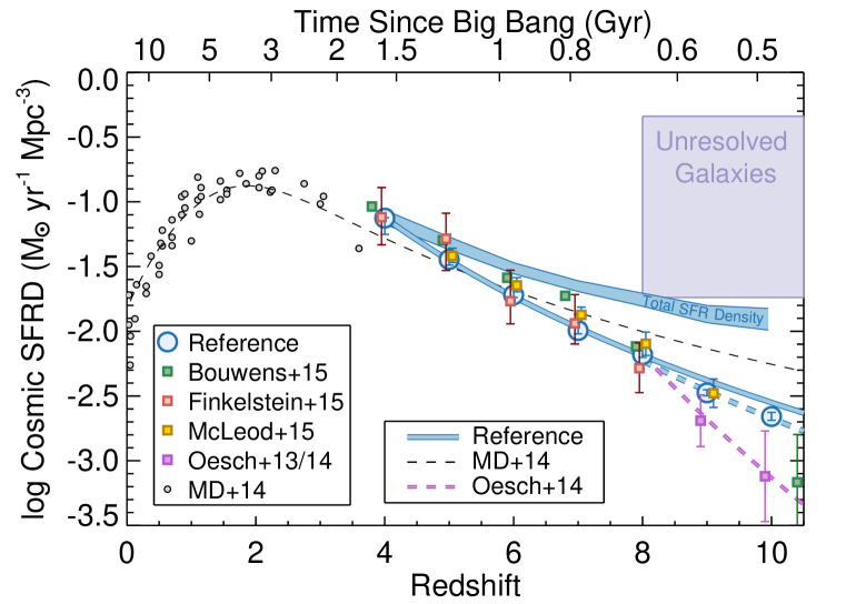
Figure 7: The evolution of the cosmic star-formation rate density, comparing the values from the integral of the reference luminosity function to those from the literature. All points have been corrected to represent a lower limit on the luminosity function integration of M${}_{\mathrm{UV}}<-$ 17, and have been corrected for dust attenuation (with the exception being the low-redshift far-infrared datapoints from Madau & Dickinson 2014). The solid blue curve shows a power-law fit to the reference data at 4 $<z<$ 8 ($\propto$[1$+z$]^-4.17±0.27), extrapolated to higher redshift, while the dashed line shows a fit only to the data at $z\geq$ 8 ($\propto$[1$+z$]^-5.10±0.69). The results from the reference luminosity function are consistent with a smooth decline in the SFR density at 4 $<z<$ 10, with no significant evidence for an accelerated evolution at $z>$ 8. However, the 68% confidence range on the total SFR density (blue shaded region; derived from integrating the reference luminosity functions to M${}_{\mathrm{UV}}=-$ 13) is consistent with an even shallower decline in the SFR density over $4<z<10$. The light purple region denotes constraints on the total luminosity density from unresolved background fluctuations (Mitchell-Wynne et al. 2015), which also imply a relatively shallow evolution of the total SFR density. The potential for a surprisingly high SFR density at $z>$ 8 will soon be settled by JWST.

5.4 The Evolution of the Cosmic Star-Formation Rate Density

A final quantity one can study with the UV luminosity function is that of the evolution of the cosmic star-formation rate density. This is derived by integrating the UV luminosity function down to a specified threshold magnitude, and then converting to a SFR using a conversion based on stellar population modeling (e.g., Madau & Dickinson 2014). As this is derived from the UV which is susceptible to dust reddening, an extinction correction also needs to be estimated and applied. As shown in a variety of previous studies, the evolution of this quantity has been shown to smoothly vary with redshift at 3 $<z<$ 8, such that the data are consistent with a single power-law $\propto(1+z)^{-(3-4)}$ (e.g., Madau & Dickinson 2014; Oesch et al. 2014; Finkelstein et al. 2015c; Bouwens et al. 2015c). The evolution to higher redshift has been less well constrained, with some observations supporting a continued smooth decline with increasing redshift at $z>$ 8 (e.g., Ellis et al. 2013; Coe et al. 2013; McLeod et al. 2015), while others report that their data require a steeper decline (e.g., Oesch et al. 2014; Bouwens et al. 2015b, c).

To explore whether the reference luminosity functions derived here can distinguish between these two scenarios, in Figure 7 I show the values of the SFR density as a function of redshift from this reference analysis, alongside values at $z<$ 4 from the compilation of Madau & Dickinson (2014). These values were derived by integrating the luminosity functions at each redshift to $-$17 (a value typically used; Bouwens et al. 2015c; Finkelstein et al. 2015c), to calculate the observed UV luminosity density. This was then converted into a SFR density using the conversion factor of 1.15 $\times$ 10^-28 M_⊙ yr^-1/(erg s^-1 Hz^-1) from Madau & Dickinson (2014). Dust corrections were derived using the redshift-dependent M_UV – $\beta$ relation from Bouwens et al. (2014, see §6.1, including at 0.35 dex scatter) coupled with the relation between dust extinction and $\beta$ from Meurer et al. (1999). Formally, the combination of these two relations can result in negative values of A_UV; these were set to zero. The total dust correction factors (L_intrinsic/L_observed) were 3.0, 2.2, 1.7, 1.4 and 1.4 at $z=$ 4, 5, 6, 7 and 8, respectively. Zero dust attenuation was assumed at $z=$ 9 and 10.

I show my results in Figure 7 alongside several results from the most recent studies at each redshift in the literature. Those literature values that were integrated to brighter limits (typically $-$17.7) were corrected down to $-$17 using the luminosity functions from each paper. Those which did not perform a dust correction had a correction applied, using the value for a given redshift derived here as discussed in the previous paragraph. We note that the reference results are consistent with those from Finkelstein et al. (2015c) and McLeod et al. (2015), while those from Bouwens et al. (2015c) are elevated at $z\leq$ 7. The latter discrepancy can be explained as the Bouwens et al. (2015c) luminosity functions are slightly elevated over those from other studies.

Madau & Dickinson (2014) found that the low-redshift evolution of the SFR density was proportional to $(1+z)^{2.7}$, while at high redshift it was proportional to $(1+z)^{-2.9}$ (fitting only to the previously available data at $z<$ 8). To explore the evolution of the SFR density implied by the reference values derived here, I fit a single power law to the reference data at 4 $<z<$ 10, finding that the SFR density is $\propto$ (1$+z$)^-4.55±0.14. Fitting to the data only at 4 $<z<$ 8, the slope is slightly shallower, (1$+z$)^-4.17±0.27, in excellent agreement with the slope of $-$4.3 found by Finkelstein et al. (2015c) over that same redshift range. The fit to the 4 $<z<$ 8 data is shown as the solid blue line in Figure 7. We extrapolate this line out to $z=$ 10, and find that it is generally in good agreement with the reference SFR density values at those redshifts, although they do appear to be slightly lower.

To explore this further, I fit a separate power law only to the data at 8 $<z<$ 10, finding a power-law slope of $-$5.10 $\pm$ 0.69. The difference between this slope and that derived from the data at 4 $<z<$ 8 is only 1.3$\sigma$. Therefore, I conclude there is no significant evidence for an accelerated evolution of the SFR density at $z>$ 8 given the currently available data. This is contrary to the evolutionary trend proposed by Oesch et al. (2014) of $(1+z)^{-10.9}$, shown by the dashed purple line, which becomes progressively more discrepant with the reference shallower evolution with increasing redshift at $z>$ 8.

I note that by forcing the assumption that each of the Schechter function parameters evolve linearly with redshift, I effectively bias the reference SFR density results to evolve smoothly with redshift. However, as shown by the excellent agreement between the data and the Schechter fits in Figure 5, the reference results supporting a smooth evolution of the SFR density are fully consistent with the data out to those high redshifts. To examine this quantitatively, I compared the fiducial results at $z=$ 9 and 10 to those from a single Schechter function fit at each redshift (holding M^∗ fixed at the $z=$ 8 value of $-$20.5 to allow the fits to converge). Comparing the goodness-of-fit via the Bayesian Information Criterion (Liddle 2004), I find no evidence that the fiducial fit is worse than when fitting the $z=$ 9 and 10 luminosity functions without the assumption of linear evolution. Therefore, I conclude that this assumption is not biasing these results.

As a final point here, I emphasize that a decline in this quantity – the SFR density for galaxies with M${}_{\mathrm{UV}}\leq-$17 – is not unexpected, as we are comparing SFR densities above a fixed absolute magnitude. As the luminosity function evolves with redshift, a progressively smaller fraction of the total UV luminosity density will come from galaxies with UV absolute magnitudes fainter than $-$17 due to the steepening of the faint-end slope. Assuming that the luminosity function extends with the measured faint-end slope down to M${}_{\mathrm{UV}}=-$13, the SFR density derived at M${}_{\mathrm{UV}}<-$17 is $\sim$60% of the total SFR density at $z=$ 6, yet only $\sim$20% at $z=$ 10. Thus, in the regime of an evolving luminosity function, the choice of the limiting magnitude directly affects the inferred evolution in the SFR density.

To illustrate this point, the shaded blue region in Figure 7 shows the 68% confidence range on the total SFR density from the reference UV luminosity functions (integrated down to $M=-$13). This is observed to evolve only very shallowly from $z\sim$ 4 – 8, leaving open the intriguing possibility that there is significant star formation hiding below our current detection limits at $z=$ 10. A resolution of this issue will require a more robust measurement of the total SFR density at $z=$ 10, which we will have in just a few years with the launch of JWST. A JWST deep field should be able to detect galaxies down to M${}_{\mathrm{UV}}=-$16 at $z=$ 10; more than 1.5 magnitudes fainter than the currently available sample of galaxies. However, the recent detection of near-infrared background fluctuations in the CANDELS GOODS-S field (Mitchell-Wynne et al. 2015) imply a total UV luminosity density at $z>$ 8 consistent with our estimate of the total SFR density, thus substantial star-formation activity at $z>$ 8 may yet be found.

6 The Physical Properties of Distant Galaxies

While the UV luminosity function can allow us to probe the global mechanisms affecting the evolution of galaxies, we can obtain a deeper insight into galaxy evolution by directly measuring galaxy physical properties. In this section I highlight two areas of significant recent activity: the chemical enrichment of galaxies, and the growth of galaxy stellar masses.

6.1 Dust Attenuation and Chemical Enrichment

One of the most direct, and straightforward measures of galaxy evolution is the evolution of galaxy colors. Although the interpretation of these colors requires assumptions and/or modeling, the direct measurement is unambiguous, and can be done with a simple photometric catalog. At lower redshift, simple color-color or color-magnitude plots are immensely useful to probe the star-forming properties of galaxies, as galaxy populations typically separate out into the star-forming “blue cloud”, and the relatively quiescent “red sequence”. At $z>$ 6, when the universe was less than 1 Gyr old, our HST observations probe only the rest-frame UV, thus our color diagnostics are somewhat more limited than at lower redshift (though we don’t expect a large fraction of quiescent galaxies, e.g., Muzzin et al. 2013; Nayyeri et al. 2014).

However, the rest-frame UV can provide robust constraints on the dust content in distant galaxies. While one would prefer to directly probe the metallicities of such systems to track chemical enrichment, in practice this is difficult with current technology. However, as dust grains are made from the heavy elements which form in stars, the build-up of dust in the universe tracks the build-up of metals. Additionally, although dust is not unique in reddening the rest-frame UV colors of galaxies, the change in UV color with increased dust content is larger than that with a comparable increase in metallicity or stellar population age (particularly at $z>$ 6, as stars must be younger than the age of the universe). Thus, tracking the evolution of the UV colors of distant galaxies provides an excellent path for following the evolution of the dust content in these systems, therefore providing a proxy to track the build-up of heavy metals in the universe.

Rather than using a single pair of filters, the rest-frame UV color is typically parameterized by the UV spectral slope $\beta$, which is defined as $f_{\lambda}\propto\lambda^{\beta}$ (Calzetti et al. 1994). The quantity $\beta$ is an excellent tracer of dust extinction, as it has been found to be well correlated with the ratio of the far-infrared to UV flux at both low and moderate redshift (e.g., Meurer et al. 1999; Reddy et al. 2012), though the exact shape of this correlation depends on the dust attenuation curve (e.g., Capak et al. 2015) and other factors (e.g., Wilkins et al. 2012, 2013). Earlier work showed that $\beta$ became substantially more negative (i.e., bluer UV colors) with increasing redshift, from $\beta\sim-$1.5 at $z\sim$ 2 to $\beta\sim-$2 at $z\sim$ 6 (e.g., Bouwens et al. 2009).

6.1.1 Colors of Faint Galaxies

Measurements at higher redshift required the deep near-infrared imaging discussed in §3.1. The earliest results on the UV colors of $z\geq$ 6 galaxies focused on faint galaxies at $z\sim$ 7, using the first year of data from the HUDF09 program (which, targeting a small field to a deep magnitude limit, was well-suited to address faint galaxies). Bouwens et al. (2010b) measured $\beta=-$3.0 $\pm$ 0.2 for faint (M${}_{\mathrm{UV}}=-$ 18) galaxies at $z\sim$ 7. They postulated that this extremely blue color may imply very low metallicities, as even young, dust free populations have $\beta\geq-$2.7 when nebular emission is accounted for. Using the same imaging dataset, Finkelstein et al. (2010) also found $\beta=-$3.0, but with a significantly higher uncertainty, of $\pm$ 0.5. Given the larger uncertainty, they concluded there was no evidence for “exotic” stellar populations, as the measured colors were consistent with local blue galaxies within a significance of 2$\sigma$.

Further evidence for “normal” stellar populations in faint galaxies at $z\sim$ 7 came from Dunlop et al. (2012). They ran simulations which showed that faint galaxies exhibit a bias, providing measurements which are bluer than the true colors of galaxies. This occurs because the colors which are used to measure $\beta$ are the same colors used to select the galaxy sample. In particular, at $z=$ 7, the HST/WFC3 $J$ and $H$ bands were used by these initial studies to measure the colors, and they were two of the only three bands with detections. If one imagines a scenario of a faint galaxy with an intrinsic $\beta=-$2 where the position of the galaxy in the $J$-band image falls on a positive noise spike, the color will be measured to be bluer than the true value. There is an equal probability that a noise spike would occur at this position in the $H$-band image, providing a color measured which is redder than the true value. However, a redder color would may push the galaxy out of the LBG selection box (or, equivalently, push more of its redshift probability distribution function to lower redshifts), thus, galaxies biased red may not make it into the galaxy sample, providing a net blue bias. Correcting for this, Dunlop et al. (2012) found no significant evidence that faint $z=$ 7 galaxies have $\beta<-$2, similar to blue star-forming galaxies at lower redshifts, a result which was confirmed by Rogers et al. (2013), who ran further simulations as well as justifying the benefits of the eventual inclusion of the F140W filter from the UDF12 program. A similar result was found by Wilkins et al. (2011).

Further progress was made with the addition of the CANDELS and UDF12 imaging. In addition to much larger samples of galaxies, more attention was put into the measurement of $\beta$ itself. Finkelstein et al. (2012b) showed that measuring $\beta$ with a single color resulted in much larger uncertainties than when using multiple colors, obtaining $\beta$ either via a power-law fit to all available colors (e.g., Castellano et al. 2012; Bouwens et al. 2012, 2014), or by fitting $\beta$ directly to the best-fitting stellar population model (Finkelstein et al. 2012b). Both Finkelstein et al. (2012b) and Bouwens et al. (2012, 2014) made use of these much larger datasets to increase the robustness of constraints on the evolution of $\beta$. Both studies found that the updated sample (as well as measurement techniques) resulted in colors of faint $z=$ 7 galaxies which did not require exotic stellar populations ($\beta\sim-$2.3 to $-$2.4, correcting for any biases). A qualitatively similar result was found by Dunlop et al. (2013), who obtained a bias-free measurement of $\beta$ for faint galaxies by leveraging observations in a new WFC3/IR filter (F140W), finding $\beta\sim-$2.1 for faint galaxies. From the combination of these above studies, one can thus conclude that even the faintest galaxies we can see at $z\sim$ 7 have colors which imply the presence of some metals, although not much dust, and therefore do not represent truly primordial systems. Such systems, if they exist, remain to be found with JWST.

6.1.2 Colors of Bright Galaxies

The large dynamic range in luminosity and stellar mass of the galaxy samples studied by Finkelstein et al. (2012b) and Bouwens et al. (2012, 2014) allowed further redshift and luminosity/stellar mass dependent trends to be explored. Bouwens et al. (2012, 2014) explored the dependance of galaxy colors on UV luminosity, and found a significant color-magnitude relation, where brighter galaxies are redder than fainter galaxies at a given redshift. Finkelstein et al. (2012b) explored the correlation of colors with stellar mass, and found that at a given redshift, more massive galaxies are redder than less massive galaxies. They concluded that this was likely a manifestation of the mass-metallicity relation seen at lower redshift (e.g., Tremonti et al. 2004; Erb et al. 2006), where more massive galaxies have higher gas-phase metallicities. The interpretation is that lower-mass galaxies are more susceptible to losing their metals (and dust) in outflows due to their shallower gravitational potentials, thus a mass (or luminosity) dependent rest-frame UV color would be an expected signature of this physical process was in place at early times. More generally, both Finkelstein et al. (2012b) and Bouwens et al. (2012, 2014) found that the average dust attenuation in galaxies rises with decreasing redshift, from near-zero at $z\sim$ 7, to A${}_{\mathrm{V}}\sim$ 0.5 at $z=$ 4.

Perhaps the most interesting result from these studies are the colors of not the faintest galaxies, but the brightest/most massive galaxies. Finkelstein et al. (2012b) found that the most massive galaxies have a roughly constant value of $\beta$ from $z=$ 4 to 7, of $\beta\sim-$1.8, similar to what Bouwens et al. (2012, 2014) found for the brightest galaxies at these redshifts. Rogers et al. (2014) found a similar result for the brighest galaxies at $z\sim$ 5. Similarly, via SED fitting, Finkelstein et al. (2015b) found that bright galaxies at $z=$ 4–7 have similar values of $E(B-V)$, of $\sim$0.1-0.15 (A${}_{\mathrm{V}}=$ 0.4–0.6 assuming a Calzetti et al. 2000 attenuation curve). The significant dust content in these galaxies is consistent with the apparently ubiquitous strong [O iii] emission implied by Spitzer/IRAC colors in many distant galaxies (e.g., Finkelstein et al. 2013; Smit et al. 2014; Oesch et al. 2015b). As shown by Finkelstein et al. (2013), galaxies with very strong [O iii] emission must have low enough stellar metallicities such that the stellar emission is hard enough to excite the oxygen in the ISM to this state, yet must have high enough gas-phase metallicities such that enough oxygen is available in the ISM. For the particular galaxy studied with an [O iii] EW of 600 Å, they found that the stellar metallicity was likely $\sim$0.2–0.4 Z_⊙, consistent with the modest levels of dust attenuation observed in these bright systems.

6.1.3 Implications of Dust at Early Times

The presence of dust in bright/massive galaxies at such early times implies that whatever mechanism dominates the creation of dust in distant galaxies is already in place by $z\sim$ 7, only $\sim$750 Myr after the Big Bang, and only 500 Myr after $z=$ 15, a reasonable guess for the epoch of the first galaxies. Finkelstein et al. (2012b) postulated that the presence of significant dust at $z\sim$ 7 implied that dust production was dominated by supernovae which have been occurring since the epoch of the first stars, assuming that stars with masses of 2–4 M_⊙, which are the most efficience dust producers when in the AGB phase, have not yet had time to evolve (Gall et al. 2011, and references therein). However, low-metallicity stars can enter the AGB phase much sooner (e.g., Maraston 2005; Karakas & Lattanzio 2014), and grain growth in the ISM can occur at arbitrarily early times, as soon as the ISM is enriched (e.g., Michałowski et al. 2010; Mancini et al. 2015), thus the picture is more muddled than originally thought.

However, if dust can be found to be present at even earlier times, that can begin to constrain the mechanisms of dust production in the early universe. Dunlop et al. (2013), using the UDF12 dataset, found $\beta=-$1.8 $\pm$ 0.6 for faint galaxies at $z=$ 9. While this is consistent with the red colors of bright/massive galaxies at $z=$ 4–7, it is also quite uncertain, thus conclusions are difficult. Wilkins et al. (2015) recently leveraged Spitzer/IRAC detections of several $z=$ 9 and 10 candidate galaxies to place the first constraints on UV colors out to $z=$ 10, finding colors only slightly bluer than similarly luminous galaxies at lower redshift. These results hint that even at $z\approx$ 10, only 500 Myr from the Big Bang, and 200 Myr from $z=$ 15, dust may be present. While a definitive conclusion will certainly require JWST, these initial hints of dust production at $z\gtrsim$ 10 provide a tantalizing glimpse into the early production of heavy elements.

6.2 The Growth of Galaxies

6.2.1 Galaxy Stellar Masses

The distribution function of galaxy stellar masses is also a useful tool to probe the galaxy physics discussed in §5.1. In particular, comparing the slope of the low-mass-end of the stellar mass function to that of the underlying dark matter halo mass function can provide an impression of the impact of feedback (supernovae, or stellar radiative) on the suppression of star formation. This has the advantage over the UV luminosity function in that it directly probes an intrinsic galaxy property without the troubling effect of dust. However, the measurement of galaxy stellar masses is an inferred quantity, therefore the galaxy stellar mass function is a less direct quantity to measure than the UV luminosity function. I will not discuss here the detailed methods for the measurements of galaxy stellar masses, but a recent review is available in Conroy (2013). In general, with decent photometry, galaxy stellar masses can be measured accurately to within a factor of a few, typically a higher accuracy than other photometrically-determined properties (though a changing initial mass function can result in a much larger systematic uncertainty in the stellar mass).

The optical and near-infrared imaging typically used to discover distant galaxies probes only the rest-frame ultraviolet, and is thus dominated by the most massive stars present in these galaxies. Stellar masses measured using only these filters can be subject to the “outshining” phenomenon, where an older, perhaps more massive population is “outshone” by a more recent episode of star-formation at the observed wavelengths. Robust stellar mass measurements thus require longer wavelength imaging. While rest-frame near-infrared imaging would be desirable, this falls longward of 10 $\mu$m at $z>$ 6, and is thus presently inaccessible. However, rest-frame optical imaging can still constrain moderately older populations, and is supplied by Spitzer/IRAC imaging at 3–5 $\mu$m at these redshifts. Direct detections at these wavelengths are not necessarily required, as if the IRAC upper limits occur at similar flux levels as the optical/near-infrared detections, useful constraints on the stellar mass can still be obtained (by, e.g., ruling out a massive older population, which would exceed the IRAC upper limits).

Individual galaxy stellar masses were determined for galaxies at $z=$ 6 from a variety of studies. In particular, Yan et al. (2005, 2006) and Eyles et al. (2007) studied $i$-band dropout galaxies in the HUDF and/or GOODS fields which had clear IRAC detections, and found that they had stellar masses of $\gtrsim$10¹⁰ M_⊙, surprisingly high for only $\sim$1 Gyr after the Big Bang. Stark et al. (2009) also measured stellar masses for a sample of a few dozen $z\sim$ 6 galaxies. They were not all detected in IRAC, thus the typical stellar masses were lower, $\sim$10⁹ M_⊙ for galaxies with M${}_{\mathrm{UV}}=-$20 to $-$21, though there was a significant scatter with some galaxies as massive as 10¹⁰ M_⊙. These massive galaxies with IRAC detections were fit with strong 4000 Å breaks, indicative of a dominant population of older stars ($\sim$500 Myr; e.g., Eyles et al. 2007). At higher-redshift, Finkelstein et al. (2010) measured the stellar masses for $\sim$30 $z=$ 7–8 galaxies in the HUDF (though see Egami et al. 2005 for an earlier mass measurement of an individual lensed $z\sim$ 7 candidate galaxy). As these galaxies were typically faint, they were mostly not detected in IRAC, and had correspondingly low stellar masses of $\sim$10⁹ M_⊙, an order of magnitude less massive than that of an L^∗ galaxy at $z=$ 3, though intriguingly similar to the masses of narrowband-selected LAEs at $z=$ 3–6. Labbé et al. (2010) found similar stellar mass results in a stack of $z=$ 7–8 galaxies in the HUDF, but through a stacked analysis was able to measure a significant average IRAC flux for these galaxies, inferring a somewhat surprising age of 300 Myr, implying that the majority of stars in these galaxies formed prior to $z=$ 10.

One complicating issue to the inclusion of IRAC photometry in these fits is the potential for a significant contribution from nebular emission lines. In particular, if the [O iii] $\lambda\lambda$4959,5007 and/or H$\alpha$ emission were strong enough, they could add significantly to the bandpass-averaged flux in the IRAC bands. This was initially not thought to be a problem, as the majority of low-redshift star-forming galaxies do not show extremely strong lines, and thus these lines were not accounted for in these initial studies. However, a bevy of observational results have since shown that high-EW [O iii] and H$\alpha$ emission is common, if not ubiquitous amongst distant star-forming galaxies, possibly indicating changes in the physical environments of typical star-forming regions (e.g., Schaerer & de Barros 2009, 2010; Finkelstein et al. 2009, 2011; Shim et al. 2011; Stark et al. 2013; Labbé et al. 2013; Song et al. 2014, 2015; Salmon et al. 2015; Smit et al. 2015; Finkelstein et al. 2015a). These strong lines boost the IRAC flux, mimicking the presence of a strong 4000 Å break, causing one to infer a higher mass and/or older population than may be correct. Schaerer & de Barros (2009, 2010) showed that by including nebular lines in the stellar population modeling process much lower stellar masses and stellar population ages can be obtained, with ages as young as 4 Myr possible for the stacked photometry of faint $z\sim$ 7 galaxies from Labbé et al. (2010). Salmon et al. (2015) quantified this further, finding that when including nebular emission lines, the stellar masses of $z\sim$ 6 galaxies in the CANDELS/GOODS-S field were systematically measured to be $\sim$20–30% lower than when emission lines were ignored.

Turning to the distribution of stellar masses, the first full, completeness-corrected stellar mass functions at $z\geq$ 6 were published by González et al. (2011). They found low-mass-end slopes which were surprisingly shallow, with $\alpha=-$1.44 at $z=$ 6 and $-$1.55 at $z=$ 7, compared to simulations at the time, which often predicted $\alpha<-$2 (e.g., Jaacks et al. 2012a). The observations thus implied that the implementation of feedback in the simulations was possibly too weak. However, these initial results were based on small samples of only $\sim$60 galaxies total at $z=$ 6 and 7 combined, and also did not include the impact of nebular lines. Recently, three separate studies on the stellar mass function have been completed using a combination of different subsets of the CANDELS data with the HUDF. Duncan et al. (2014) used the CANDELS GOODS-S field to find much steeper faint-end slopes of $\sim-$1.9 at these redshifts. Grazian et al. (2015) used both the CANDELS GOODS-S and UDS fields, to find a similarly steep slope at $z=$ 7, though they found $\alpha=-$1.55 at $z=$ 6. The most recent study, by Song et al. (2015) also used two CANDELS fields (GOODS-N and GOODS-S), but made use of deeper IRAC data newly available from the S-CANDELS survey (PI Fazio). By using simulations to verify that their methods minimized systematic offsets in their results, Song et al. (2015) found that the low-mass-end slope $\alpha$ steadily becomes steeper, from $-$1.53 at $z=$ 4 (similar to González et al. 2011) to $-$2.05 at $z=$ 7. At the highest redshifts, this slope is similar to that of the dark matter halo mass function, implying that feedback may be less efficient at suppressing star formation towards higher redshift.

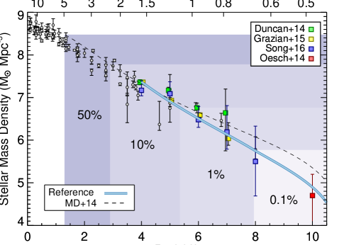
Figure 8: The evolution of the total stellar mass density in the universe, all derived assuming a Salpeter IMF. The low redshift measurements have a range of definitions, but I note that all high redshift measurements were obtained by integrating stellar mass functions from 8 $<logM/M$_⊙$<$ 13 (the flatter slope of the low-mass end of the stellar mass function at $z<$ 4 implies that the lower limit of the integration is less important). The gray points show the data from the compilation of Madau & Dickinson (2014), while the other symbols come from recent estimates of the stellar mass function at high redshift, defined in the legend. The blue and dashed black curves show the stellar mass density obtained by integrating the SFR density evolution from Figure 7. The left side of the shaded regions denote the redshift at which the total stellar mass density formed is equal to the listed percentage of the $z=$ 0 value.

The integral of the stellar mass function provides the stellar mass density of the universe at a given epoch. As measurements at very low-redshift from, e.g., the SDSS, are quite robust, it is interesting to compare the stellar mass density at high redshift to low, to investigate what fraction of the total stellar mass of the universe exists at a given epoch. This has been done in a variety of studies, (e.g., Dickinson et al. 2003; Rudnick et al. 2003; Duncan et al. 2014; Grazian et al. 2015; Oesch et al. 2015b), which are highlighted in Figure 8. In this figure I also show the stellar mass density obtained by integrating the evolution of the SFR density from Figure 7, showing both the updated reference trend from this work, as well as the values from Madau & Dickinson (2014). At $z<$ 2, the stellar mass density derived in this way is systematically higher by a small amount than that obtained directly from stellar mass measurements. Madau & Dickinson (2014) discussed a number of possible causes for this offset, including overestimation of the star-formation rates (which could be the case if, for example, galaxies have a dust attenuation curve similar to the Small Magellanic Cloud), or underestimation of the stellar masses (due to lack of constraints on older stars, and/or an evolving IMF). However, at $z>$ 3, our integrated SFR density shows excellent agreement with the observations of Grazian et al. (2015), Song et al. (2015) and Oesch et al. (2014). The values from Duncan et al. (2014) show a modest significant difference at $z\geq$ 5 due to their much steeper low-mass end slope (see discussion in Song et al. 2015, and also Graus et al. 2015). By comparing the values of my model at a given redshift to that at $z=$ 0, I find that the universe formed 50% of its stellar mass by $z\sim$ 1.3, with $\sim$10%, 1%, 0.1% and 0.01% of the stellar mass in place by $z=$ 2.9, 5.4, 8.0 and 10.2, respectively. Observations have therefore tentatively inferred the presence of 99.99% of all the stellar mass which has ever formed in the universe, though much of it remains to be directly detected.

6.2.2 Star-Formation Histories

While the measurement of the instantaneous stellar mass is relatively straightforward, teasing out the growth of that stellar mass with time is more difficult. When measuring stellar population properties via SED fitting, the star-formation history (SFH) is typically assumed to follow some functional form. Initial studies assumed a SFH which declined exponentially with time (so-called tau models), which successfully works at late times when many galaxies are in the process of quenching and gas inflow is likely less than at higher redshifts (e.g., Maraston et al. 2010, and references therein).

However, several years ago it was noted that this assumption may not be valid at higher redshifts. Maraston et al. (2010) found that exponentially declining models produced extremely young ages for a sample of $z\sim$ 2 star-forming galaxies, while “inverted-tau” models (where the SFR increases exponentially with time) produced more realistic results. Papovich et al. (2011) also found that, by linking galaxies from $z=$ 8 to $z=$ 3 using a constant number density tracking technique (e.g., van Dokkum et al. 2010; Leja et al. 2013; Behroozi et al. 2013a; Jaacks et al. 2015), galaxies on average have rising star-formation histories (see also Salmon et al. 2015). Reddy et al. (2012) reached a similar conclusion by comparing SED-fitting derived SFRs to UV$+$IR SFRs, finding that when a declining SFH was assumed, the SED-fitting derived SFR was too low. A bevy of theoretical studies have reached similar conclusions: at $z\gtrsim$ 3, the average SFRs of galaxies grow roughly steadily with time (e.g., Finlator et al. 2007, 2011; Jaacks et al. 2012b).

Such growth cannot continue unchecked. In particular, at $z\lesssim$ 3 galaxies begin to quench, thus clearly such a rising SFH is not appropriate for all galaxies at all times. In an advanced MCMC analysis of galaxy evolution from $z=$ 8 to 0, Behroozi et al. (2013b) found that while galaxies at $z>$ 3 appeared to have SFRs which increased with time as a power law (similar to Papovich et al. 2011, though with a steeper exponent), at $z\sim$ 2-3 there existed a mass-dependent redshift where the SFHs began to turnover and decline. This turnover occurs as late as $z=$ 0.5 for lower-mass galaxies, thus even at relatively low redshift there may be a mix of rising and falling SFHs. They proposed either a double power law SFH (Eqn. 23 in Behroozi et al. 2013b), or a combination of a power-law and declining exponential, either of which should be appropriate for galaxies at any epoch.

Finally, I note that the majority of the discussed studies are considering ensembles of galaxies, therefore the SFHs which were derived represent the average growth of stellar mass in these galaxies. The SFH for any individual galaxy may be quite stochastic, depending on a variety of effects, including environment, merger activity, gas accretion, etc. Thus, caution should be used when considering the evolution of individual galaxies.

6.2.3 Evolution of Galaxy Specific Star-Formation Rates

The specific star-formation rates (sSFR; SFR/stellar mass) of galaxies are an excellent tracer of galaxy growth, as this quantity normalizes the growth of new stars by the current stellar mass. Theoretical simulations predict that the sSFR at fixed stellar mass should be rising with increasing redshift, as such models predict that star formation is governed by cold gas accretion, and should therefore increase with increasing redshift (e.g., Neistein & Dekel 2008; Davé et al. 2011; Krumholz & Dekel 2012). It was thus surprising when the first measurements of the evolution of the sSFR at high redshift showed it to be roughly flat from $z\sim$3 to 7 (González et al. 2010). Subsequent work by Stark et al. (2013) considered the impact of nebular emission, which was not accounted for in González et al. (2010), and found hints that the sSFR may be rising from $z=$ 5 to 7. González et al. (2014) performed an updated analysis with a larger sample, including nebular lines and varying SFHs (including those which increase with time) and also found evidence for a rising sSFR with increasing redshift, though with a redshift dependance much weaker than simulations.

Most recently, Salmon et al. (2015) found a steeper increase in sSFR with increasing redshift from $z=$ 4–6. Their fiducial analysis tracking galaxies at constant mass was not a great match to simulations, but when they instead considered tracking galaxies with an evolving cumulative number density to more accurately track progenitors and descendants (Behroozi et al. 2013a), they found an excellent match to both Neistein & Dekel (2008) and Davé et al. (2013) in both normalization and slope. Therefore, at present there is no significant discrepancy with models at high redshift. However, current results at $z>$ 4 have large uncertainties, and, at the highest redshifts, are based on small samples, thus there is room for improvement. Additionally, there is a significant discrepancy between models and observations at 0.5 $<z<$ 2 (see Fig. 9 of González et al. 2014), where observed sSFRs evolve shallowly down to $z\sim$ 1 then fall off quickly towards lower redshift, while simulations predict a smoother evolution. Thus, the evolution of the sSFR will likely remain an active area of inquiry at all redshifts.

6.2.4 Evolution of the Stellar-Mass to Halo-Mass Ratio

As a final consideration into the growth of galaxies, I consider the dependance of galaxy growth on the underlying dark matter halo mass. Because the growth of dark matter halos is well understood via simulations such as the Millenium, Bolshoi, and Illustris projects (e.g., Springel et al. 2005; Klypin et al. 2011; Vogelsberger et al. 2014), linking galaxies to these halos can allow us to gain insight into the efficiency with which galaxies turn gas into stars. A common way to do this is to calculate the stellar mass to halo mass (SMHM) ratio. The halo mass can best be observationally inferred via galaxy clustering, which allows one to estimate the dark matter halo mass for a specific sample of galaxies by comparing their spatial distribution to the underlying dark matter halo distribution. In practice, this requires large samples of galaxies, particularly if one wishes to split their sample into several bins by, for example, stellar mass (see Overzier et al. 2006 and Barone-Nugent et al. 2014 for initial measurements at $z\geq$ 6). Lacking sufficient galaxy numbers, an alternative method has been derived known as abundance matching (e.g., Moster et al. 2010; Behroozi et al. 2010). This technique assumes that a galaxy property (for example, the stellar mass, or UV luminosity) is a monotonic function of the halo mass, such that the most massive/luminous galaxies live in the most massive halos. One can then match a galaxy distribution function (i.e., the stellar mass or UV luminosity function) to a dark matter halo mass function, linking galaxies to halos at a constant cumulative number density, to derive the halo mass for a given stellar mass or UV luminosity.

Behroozi et al. (2013b) used abundance matching (as part of their MCMC analysis considering a wide range of observables) to constrain the evolution of the SMHM relation from $z=$ 0 to 8. They found the interesting result that this relation seems roughly constant from $z=$ 0 to 4, with a peak SMHM ratio of $\sim$1-2% at halo masses of $\sim$10¹² M_⊙. There are two interesting points to take away from this. First, the apparent constant halo mass where the SMHM reaches its peak value implies that there is a characteristic halo mass where galaxies form stars most efficiently. At lower and higher halo masses, the feedback effects discussed in §5 are likely stronger (at least at $z<$ 4). Second, the peak ratio of $\sim$1-2% is much lower than the cosmic fraction of available baryons in halos, which should be $\sim$17% (for WMAP7 cosmology, Komatsu et al. 2011). Thus, galaxies are not efficient star formers, as the majority of gas does not make it into stars. Behroozi et al. (2013b) continued this analysis to $z>$ 4, finding that the SMHM relation began to evolve, in that at a constant halo mass, a $z>$ 4 galaxy will have a higher stellar mass than at lower redshift, perhaps implying a change in the efficiency governing star formation.

This result was based on very early observational results at $z>$ 6, including pre-2013 luminosity and stellar mass functions, which differ significantly from the most recent results. Finkelstein et al. (2015b) performed an updated, albeit much simpler, analysis, performing abundance matching using their updated luminosity functions. They derived the halo mass at M${}_{\mathrm{UV}}=-$21 at $z=$ 4–7 (approximately L^∗ at these redshifts), finding that the halo masses were lower (by 0.6 dex) at $z=$ 7 compared to $z=$ 4. Measuring the stellar masses for these bright galaxies, they found them to remain roughly constant across this redshift range (log M/M_⊙ $\sim$9.6–9.9), thus the SMHM ratio of galaxies at this constant luminosity/stellar mass increased towards higher redshift. Normalizing by the cosmic abundance of baryons, they found that the fraction of baryons converted into stars in these galaxies was roughly 2.3$\times$ higher at $z=$ 7 than at $z=$ 4, again implying that higher redshift galaxies are more efficient star-formers. This provides further evidence that the physics shaping galaxy evolution may be evolving at $z>$ 4. The explanation need not be exotic; rather, such changes may be expected, as a changing gas density, black hole accretion, and/or impact of SNe feedback may be expected as the expansion of the universe plays back in reverse. Further theorietical and observational work is needed to clarify exactly the physical processes which may be changing. In particular, these results are based entirely on the measurement of luminous matter. A direct measurement of the evolution of the gas reservoirs in these galaxies will provide a much clearer insight into how these distant galaxies are converting their gas into stars.

7 Reionization

At the time that CMB photons began their long journey to our telescopes, the universe had expanded and cooled enough for hydrogen gas to become neutral. This was the state for the next few hundred million years — a period known as the “dark ages”. Eventually, baryonic matter cooled and condensed in dark matter halos to form the first stars and galaxies in the universe. These objects provided a key source of ionizing photons, ionizing the cosmic haze of neutral intergalactic gas in a process known as reionization. Understanding how reionization proceeds, both the evolution of the neutral fraction of the IGM with time as well as its spatial variation provides key constraints on the nature of these first luminous sources in the universe. In this section I present current observational constraints on reionization, focusing on those derived directly from galaxies at $z>$ 6, with a discussion of the current limiting factors.

7.1 The Timeline of Reionization

7.1.1 Ly$\alpha$ Forest

The most robust constraints on the end of reionization comes from the measurement of the Gunn-Peterson trough in the spectra of distant quasars. By measuring the transmission in the Ly$\alpha$ forest of $z>$ 6 quasars, the neutral fraction of the IGM has been constrained to to be $\ll$1% at $z\approx$ 6 (e.g., Fan et al. 2006). As individual quasars probe only single sightlines, there are bound to be variations, and in fact Becker et al. (2015) recently measured a significant trough in a $z=$ 6.0 quasar, implying a partially neutral IGM all the way down to $z\sim$ 5.5 on that line-of-sight. Additionally, from the variations in transmission from quasar spectra, Becker et al. (2015) find that the variations in the UV background at $z>$ 5.6 require significant variations in the IGM neutral fraction. The observations do not become consistent with an IGM opacity arising from only the matter density field until $z\sim$ 5.5. Thus, while reionization is likely mostly complete by $z\sim$ 6, current observations do not constrain it to be fully complete until $z\lesssim$ 5.5. Quasars are somewhat less useful to probe deep into the epoch of reionization, however, as this measurement saturates at a relatively small neutral fraction ($\sim$10%), and only a single $z\geq$ 7 quasar is currently known (Mortlock et al. 2011).

7.1.2 Cosmic Microwave Background

Reionization is expected to be a prolonged process, with the overdense regions which formed stars first beginning the process at early times, with neutral gas lingering in the densest filaments until late times (e.g., Finlator et al. 2009). While it is difficult to obtain strict constraints on the beginning or end of reionization, measurements of the optical depth due to electron scattering from the cosmic microwave background (CMB) does provide observational constraints on the total number of free electrons along the line of sight to the CMB, which can be used to estimate the midpoint of reionization. Initial results from the Wilkinson Microwave Anisotropy Probe (WMAP) measured a large optical depth, implying a midpoint for reionization at $z=$ 17 $\pm$ 5 (Spergel et al. 2003), which led to a bevy of work imposing significant early star formation. However, subsequent analysis with additional WMAP data resulted in lower optical depths, and the latest results from Planck find $\tau_{\mathrm{es}}=$0.066 $\pm$ 0.016, implying $z_{\mathrm{reion}}=$ 8.8${}_{-1.1}^{+1.2}$ (Planck Collaboration et al. 2015), implying a later start to reionization. Thus, it appears likely that reionization started not much before $z\sim$ 10, and was predominantly completed by $z\sim$ 6.

7.1.3 Ly$\alpha$ Emission

Another probe into reionization is the measurement of Ly$\alpha$ emission from galaxies, as the resonant scattering nature of Ly$\alpha$ photons means that their detection is impaired by a significantly neutral IGM. This was initially done with Ly$\alpha$ emitters discovered via narrowband imaging surveys. The latest studies do find evidence of a drop from $z=$ 5.7 to 6.5, where Ly$\alpha$ emitters are less luminous (and/or less common) at higher redshift (e.g., Ouchi et al. 2010). Attempts to continue these narrowband studies to higher redshift have met with difficulty, as very few reliable candidates have been discovered (e.g., Tilvi et al. 2010; Krug et al. 2012; Faisst et al. 2014, ; see §3.3).

A more recent method involving Ly$\alpha$ is to perform spectroscopic follow up of continuum-selected galaxies to measure their Ly$\alpha$ emission. This is powerful as it relies on a known sample of robustly selected galaxies, and even non-detections are very constraining as one can model upper limits in the data and thus study the non-detections on a galaxy-by-galaxy basis (unlike narrowband studies, where the high-redshift galaxies are only found if they have strong Ly$\alpha$ emission). This method is possible because the fraction of continuum-selected galaxies with detected Ly$\alpha$ emission rises from $\sim$30% at $z=$ 3 to 60-80% at $z=$ 6 (e.g., Shapley et al. 2003; Stark et al. 2010, 2011). This increase is likely due to decreasing dust attenuation (§6.1), which should continue to higher redshifts, thus Ly$\alpha$ should be nearly ubiquitous amongst star-forming galaxies at $z>$ 6. An observed drop in the fraction of galaxies exhibiting Ly$\alpha$ emission (typically parameterized by comparing the EW distribution at higher redshift to that at $z=$ 6) may signal a rapidly evolving IGM neutral fraction.

As discussed in §4.2, such a drop has been exactly what has been seen. While it may be that a larger fraction of the samples are interlopers at these redshifts, that seems unlikely given the high confirmation fraction of similarly-selected $z\sim$ 6 galaxies (e.g., Pentericci et al. 2011). Converting this observed evolution of the Ly$\alpha$ EW distribution into constraints on reionization is less direct, requiring advanced modeling with a number of assumptions. In particular, one needs to know the emergent Ly$\alpha$ profile, which depends on the ISM H i column density and geometry, as well as the kinematics of the ISM. Reasonable assumptions on these properties can be made based on observations at $z\sim$ 2 (e.g., Chonis et al. 2013; Hashimoto et al. 2013; Song et al. 2014). One then needs to model the IGM, which can be done with semi-numerical models, or full-on cosmological hydrodynamic simulations (e.g., Dijkstra et al. 2011; Jensen et al. 2013). These models include not only diffuse neutral gas in the epoch of reionization, but also attenuation post-reionization from dense ionized gas. When such models are compared to observations they imply a volume-averaged neutral fraction of $\sim$50% at $z=$ 7 (e.g., Pentericci et al. 2014). This is a drastic change from the apparently fully ionized universe at $z\sim$ 6, and is too fast compared to what is seen in theoretical reionization models (see also Treu et al. 2013 and Tilvi et al. 2014 for qualitatively similar results at $z\sim$ 8). I direct the reader to the recent review on this topic by Dijkstra (2014) for more details on the modeling process.

As discussed by Dijkstra (2014), there are a number of alternatives which may allow the current observations to be consistent with a lower volume-averaged neutral fraction at $z\sim$ 7. One likely candidate is that the observed evolution is primarily due to an increase in the opacity of self-shielding Lyman limit systems. Prior to the completion of reionization, the ionizing background is smaller than just after reionization, which makes it easier for these systems to self-shield (e.g., Bolton et al. 2011; Mesinger et al. 2015). At this time, dense filaments will “thicken”, increasing the optical depth to Ly$\alpha$ photons. The galaxies we attempt to observe in Ly$\alpha$ likely lie in overdense environments, increasing the likelihood that a line-of-sight to a given galaxy will pass through one (or more) nearby filaments. Bolton & Haehnelt (2013) found that when including these systems in their models, a volume-averaged neutral fraction of only 10-20% was needed to explain the observed Ly$\alpha$ evolution (though see Mesinger et al. 2015).

A final possibility is that at least some of the observed drop in Ly$\alpha$ detectability is caused by the properties of galaxies themselves. While at lower redshift dust can significantly attenuate Ly$\alpha$, dust is unlikely to provide a higher Ly$\alpha$ attenuation at $z\geq$ 7 than at $z=$ 6 (see §6.1). However, Ly$\alpha$ is also highly sensitive to the column density of neutral hydrogen, and if the potential evolution of the SMHM relation discussed in §6.3 is due to increased gas reservoirs in galaxy, then it may be that at higher redshift more Ly$\alpha$ photons suffer additional resonant scattering within the galaxy, reducing the Ly$\alpha$ observability with current telescopes (see also Papovich et al. 2011 and Finkelstein et al. 2012a). Finally, it may be that galaxies at higher redshift have higher escape fractions of ionizing photons; every ionizing photon which escapes is one less photon which is converted into Ly$\alpha$, lowering the intrinsic Ly$\alpha$ luminosity (e.g., Dijkstra et al. 2014). However, although relatively high escape fractions have occasionally been observed (e.g., Steidel et al. 2001; Shapley et al. 2006; Iwata et al. 2009; Vanzella et al. 2010; Nestor et al. 2011), some may be due to superimposed foreground objects (e.g., Vanzella et al. 2012), and the majority of models predict that the currently observable galaxies leak essentially zero ionizing photons (e.g., Paardekooper et al. 2015; Ma et al. 2015).

Regardless of the changing IGM or ISM, the few detections of Ly$\alpha$ which we do have at $z>$ 7 implies that some combination of global or local IGM state combined with ISM geometry and kinematics will allow focused observational studies with future facilities to use Ly$\alpha$ as a spectroscopic indicator deep into the epoch of reionization.

7.2 Constraints from Galaxies

The declining quasar luminosity function at $z>$ 3 (e.g., Richards et al. 2006) has led to the conclusion that star-formation in galaxies produced the bulk of ionizing photons necessary for reionization. A key measure is thus a cosmic “census” of distant galaxies, measuring their rest-UV light, then inferring the likely ionizing photon emissivity to see if the observed star-formation at a given epoch can sustain an ionized IGM. If one assumes that galaxies do indeed provide all the needed ionizing photons, this analysis provides an independant measure into the timeline of reionization.

There are a number of assumptions which need to be made to convert rest-frame UV observations of galaxies into a constraint on reionization.

• Stellar population: As one observes non-ionizing UV photons, that observable needs to be converted to the emergent ionizing radiation, which requires assuming a stellar population. The primary considerations here are the initial mass function and the metallicity. The conversion factors do not vary wildly if one assumes a Salpeter IMF and non-zero metallicity ($\sim$ 20-30%; e.g., Finkelstein et al. 2012a). However, a changing IMF, particularly one which results in more massive stars, could produce a much higher number of ionizing photons per unit UV luminosity making it easier for galaxies to reionize the IGM.

• Escape fraction: Only ionizing photons which escape a galaxy are available to contribute to reionization, thus one needs to assume an escape fraction of ionizing photons (f_esc). This quantity cannot be directly observationally ascertained in the epoch of reionization due to attenuation along the line of sight. Studies at $z<$ 4 have found that the majority of galaxies have little-to-no escaping ionizing radiation (e.g., Siana et al. 2010), though examples of escape fractions on the order of 20% have been found (e.g., Nestor et al. 2011). Finkelstein et al. (2012a) showed that values greater than 13% at $z=$ 6 would violate the ionizing photon emissivity obtained from observations of the Ly$\alpha$ forest. Most simulations predict that galaxies massive enough to be currently observed have very low escape fractions, and values $>$20% only occur in the very lowest mass halos (e.g., Paardekooper et al. 2015). Values of $\sim$20% are frequently assumed in the literature when obtaining reionization constraints from galaxies, which may thus be optimistically too high (e.g. Finkelstein et al. 2010; Robertson et al. 2013, 2015).

• Limiting Magnitude: When integrating the UV luminosity function, one needs to assume a limiting magnitude. An absolute limit would be the magnitude of a single O star ($\sim-$5); however, galaxies likely have their star formation suppressed in more massive halos, due to photoionization of their gas from star formation in nearby halos. Galaxies are commonly observed at $z\sim$ 6–8 down to magnitudes of M_UV $=-$17, thus it may be reasonable to assume fainter values of $-$13 or $-$10, as is often done in the literature. Recent simulations have found that the luminosity function may break at M$=-$14 to $-$16 due to a combination of physical processes (Jaacks et al. 2013; O’Shea et al. 2015), or at $-$13 by simulating the progenitors of galaxies in the Local Group (e.g., Boylan-Kolchin et al. 2015). However, initial results from the Hubble Frontier Fields lensing survey show that the luminosity function continues steeply to M${}_{\mathrm{UV}}=\sim$13 at $z=$ 6 (Livermore et al. 2016), and future studies with the full Frontier Fields dataset should produce even better constraints.

• Clumping Factor of IGM: The density of gas in the IGM is a key parameter, as it is more difficult to keep dense gas ionized than diffuse gas, as the recombination time is shorter. This is typically parameterized by the clumping factor (C), where higher values of $C$ require more ionizing photons to sustain reionization. While $C$ was originally thought to be quite high ($\sim$ 30; Gnedin & Ostriker 1997), more recent models, with a better understanding of the interface between galaxies and the IGM, find lower values ($<$5; e.g., Pawlik et al. 2009; Finlator et al. 2012; Pawlik et al. 2015). The most recent models of Pawlik et al. (2015) find a clumping factor which is $<$3 at $z>$ 8, rising to $C=$4 at $z=$ 6. Most studies below assume $C=$ 3.

With these assumptions, one can use a model of reionization to determine whether the galaxy population at a given redshift can sustain an ionized IGM. The model of Madau et al. (1999) is commonly used, which calculates a redshift-dependent limiting UV luminosity density to sustain an ionized IGM, assuming a stellar population term, and values for f_esc and $C$. One can then integrate an observed luminosity function (to an assumed limiting magnitude), and compare to this model to explore the contribution of galaxies to reionization. This has been done in a variety of studies; here I will review a few recent results.

Using new samples of $z=$ 6, 7 and 8 galaxies from the CANDELS and HUDF surveys, Finkelstein et al. (2012a) examined the contribution to reionization solely from observed galaxies (i.e., with no extrapolation to fainter magnitudes). They found that if the typical galaxy had an escape fraction of $\sim$30%, then the observed population of galaxies could sustain an ionized IGM by $z=$ 6, in contrast to previous studies which found that fainter galaxies were required (e.g., Bunker et al. 2004; Yan & Windhorst 2004). By using limits on the ionizing emissivity from observations of the $z\approx$ 6 Ly$\alpha$ forest, Finkelstein et al. (2012a) found that if the UV luminosity function continues with the observed steep slope to $M_{\mathrm{UV}}=-$13, then the typical escape fraction could be no higher than $\sim$13%. However, even with this modest escape fraction, galaxies could still sustain an ionized IGM by $z=$ 6 if the luminosity function extended down to such faint magnitudes. Robertson et al. (2013) performed a complementary analysis, using not only the UV luminosity function, but also measurements of the stellar mass density and the electron scattering optical depth from the WMAP measurements of the CMB as constraints. They found similar results, in that by assuming f${}_{esc}=$ 20%, galaxies can sustain an ionized IGM by just after $z=$ 6, but that fainter galaxies would be required to complete reionization at earlier times.

Over the next few years, the advent of Planck coupled with the large improvement on the precision of the UV luminosity function from the completed CANDELS survey allowed these constraints to be tightened. Finkelstein et al. (2015c) used their updated luminosity functions to revisit the constraints placed on reionization from galaxies. Assuming a fiducial model with $C=$ 3 and f${}_{esc}=$ 13%, they found that galaxies suggest that reionization was largely complete by $z=$ 6, and that the universe was primarily neutral by $z>$ 10. Their observations constrained a midpoint of reionization (defined as the epoch when the volume-averaged ionized fraction reached 50%) of 6.7 $<z<$ 9.4 (at 68% confidence). Although this analysis did not use the recent observations from Planck as constraints, the electron scattering optical depth derived from this reionization history is in excellent agreement with the Planck observations, implying that a significant contribution to reionization from galaxies at $z>$ 10 is not needed. Robertson et al. (2015) updated their previous analysis with the Planck constraints and the latest luminosity function results, found a similar result in that a reionization process which starts at $z\approx$ 10 and completes by $z\approx$ 6 is consistent with both the observations of galaxies and the Planck observations of the CMB. Finally, Bouwens et al. (2015a) recently performed a complementary analysis, eschewing constraints from the luminosity functions of galaxies in their analysis to derive independant constraints on the ionizing sources. As constraints, they combined observations of the Ly$\alpha$ forest from quasar spectra with the Planck optical depth measurements, as well as observations of the evolving Ly$\alpha$ emission from galaxies. They derived an evolution in the ionizing background which was consistent with the ionizing emissivity derived from observations of galaxies (with $f_{esc}\sim$10-20%) even though galaxies were not used as constraints. This again suggests that galaxies are the major producers of the ionizing photons which drove the reionization of the IGM, provided such ionizing escape fractions are achievable.

7.3 Reference Reionization Constraints

The studies discussed above uniformly arrive at a similar conclusions: galaxies were responsible for reionization, and reionization completed by $z\sim$ 6. However, the time-evolution of the neutral fraction during reionization is less well constrained. For example, the constraints on the mid-point of reionization from Finkelstein et al. (2015c) of $\Delta z=$ 2.7 are largely due to the faint-end slope uncertainties from the luminosity function. As discussed in §5.3, we can improve upon these constraints with my derived reference UV luminosity function. For example, the fractional uncertainty on the faint-end slope ($\sigma_{\alpha}/\alpha$) from Finkelstein et al. (2015c) and Bouwens et al. (2015c) was 10% and 6%, respectively, while from my reference UV luminosity function at $z=$ 7 we I find $\sigma_{\alpha}/\alpha=$ 2%. Therefore, to conclude this discussion of reionization I explore the improvements in the constraints on the contribution of galaxies to reionization available when I use luminosity functions derived in §5.

To derive this reionization history, I follow the methodology of Finkelstein et al. (2015c), assuming $C=$ 3 and f${}_{esc}=$ 13% (which does not violate constraints on the Ly$\alpha$ forest at $z=$ 6). I then integrate the fiducial reference UV luminosity functions from §5.3 at each redshift to a limiting magnitude of $M_{\mathrm{UV}}=-$13 to derive the UV luminosity density, using the results from the MCMC chains to derive uncertainties on these values. Using the model of Madau et al. (1999) with the above assumptions, I then calculate the volume-averaged neutral fraction (x_HI) at each redshift, propagating through the uncertainties on the UV luminosity density to derive a 68% confidence range on x_HI. The resultant 68% confidence reionization history is shown in Figure 9.

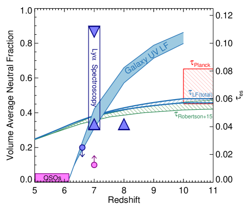
Figure 9: The volume-averaged neutral fraction as a function of redshift, with the 68% confidence range on constraints from the integral of the reference UV luminosity functions shown by the shaded blue region. An upper limit from the Ly$\alpha$ narrowband survey by Ouchi et al. (2010) is shown by the blue circle, while constraints via Ly$\alpha$ spectroscopy at $z=$ 6.5–7 by Pentericci et al. (2014) and at $z=$ 7.5–8 by Tilvi et al. (2014) are shown by the blue arrows. Constraints via quasars are shown by the magenta regions (from Fan et al. 2006 at $z<$ 6, and Bolton et al. 2011 at $z=$ 7). The Thomson optical depth to electron scattering derived from the reference UV luminosity function constraints is shown by the hatched blue region, and is consistent with constraints from Planck, shown by the hatched red region (both corresponding to values on the right-hand vertical axis), as well as the recent study by Robertson et al. (2015) shown in green. This fiducial reionization history constrains reionization to be $<$10% complete by $z\sim$ 10, and $>$85% complete by $z\sim$ 7.

The tighter constraints on the luminosity functions available when using all available data lead to more constraining results on the evolution of the volume averaged neutral fraction x_HI than previous studies utilizing only galaxy data. This analysis constrains x${}_{\mathrm{HI}}=$ 0% at $z=$ 6 and x${}_{\mathrm{HI}}>$ 80% at $z=$ 10, with the 68% confidence constraint on the midpoint of reionization being 7.3 $<z<$ 7.7. I calculated the Thomson optical depth to electron scattering from both my upper and lower 68% confidence constraints on the neutral fraction, finding $\tau_{es}=$ 0.057 – 0.060 (blue hatched region in Figure 9). This is in consistent with the low end of the observational constraints from Planck of $\tau_{es}=$ 0.066 $\pm$ 0.012. This is particularly striking as the Planck measurements were not used as an input constraint on the galaxy luminosity function-based reionization history. Rather, the galaxy observations, combined with assumptions on the limiting magnitude, clumping factor, and escape fraction, produce a result which is consistent with the Planck observations. The results found here are highly consistent with those from Robertson et al. (2015), as shown by the green shaded region in Figure 9. If the true value of $\tau_{es}$ is closer to the higher end of the Planck constraints, it could leave room for modest star-formation activity at $z>$ 10, while if it is closer to the value implied by our observations at the lower end of the Planck constraints, it leaves little room for a significant number of free electrons at higher redshift.

Comparisons to other complementary observations are also shown in Figure 9. Current results from quasars imply a fully ionized universe at $z<$ 6 (e.g., Fan et al. 2006), while the single known quasar at $z=$ 7 implies a volume averaged neutral fraction $>$10%. On the other hand, Ouchi et al. (2010) found x${}_{\mathrm{HI}}<$ 20% at $z=$ 6.6, using the observed evolution of the Ly$\alpha$ luminosity function via narrowband imaging. Using the incidence of Ly$\alpha$ emission in spectroscopic followup of known high-redshift sources, Pentericci et al. (2014) and Tilvi et al. (2014) constrained 30% $<x_{\mathrm{HI}}<$ 90% at $z=$ 7, and x${}_{\mathrm{HI}}>$30% at $z=$ 8, respectively. While both the quasar and Ly$\alpha$ luminosity function-derived constraints are fully consistent with my inferred reionization history, taken at face value the $z=$ 7 Ly$\alpha$ results are in modest tension. These studies imply a significant neutral fraction of $>$30% by $z=$ 7, while the luminosity functions seemingly allow at most 20% of the IGM to be neutral.

However, there is presently enough uncertainty in all of these measures such that the tension can be easily resolved. For example, reducing the assumed escape fraction to 10% increases the neutral fraction at $z=$ 7 to be consistent with the lower limit from Pentericci et al. (2014), while still generating enough free electrons to satisfy the Planck constraint. Likewise, the constraints via Ly$\alpha$ spectroscopy are relatively poor, due both to small sample sizes as well as modeling uncertainties, both which should improve significantly in the coming years as observers build up more robust samples of $z>$ 7 spectroscopic observations. The escape fraction is likely the biggest wild card, and while here I impose an upper limit set by Ly$\alpha$ forest constraints at $z=$ 6, we have no reasonable constraint on the lower limit of this quantity. Future studies at $z=$ 2–3, as well as more advanced modeling, should shed light on this issue in the coming years. Should the escape fractions be universally lower than currently assumed, it may be that galaxies play less of a role in reionization than is currently thought, opening the door for a larger contribution from low-luminosity AGN (e.g., Giallongo et al. 2015; Madau & Haardt 2015).

8 Prospects over the coming decade

In this review I have focused on the extensive knowledge we have gained about the distant universe via observations. Galaxy surveys can now discover galaxies out to redshifts greater than 10, with spectroscopic redshifts now possible out to $z>$ 8. The shapes of the galaxy rest-frame UV luminosity functions at $z=$ 4–7 have become highly constrained, enabling their use as tools to study galaxy evolution. Deep mid-infrared photometry allows robust stellar masses to be measured out to $z>$ 8, perhaps accounting for the first 0.01% of the stellar mass to ever have formed in the Universe. A better understanding of the dust attenuation in galaxies allows us to not only better track the build-up of heavy elements in the distant universe, but also, combined with robust estimates of the luminosity function faint-end slope, to constrain the total amount of star-formation at each epoch, which may remain relatively flat out to $z=$ 8 with a possible decline at higher redshift.

The exquisite observational results which have been summarized here are representative of the truly outstanding amount of resources, both human and technological, which have been applied to this epoch in the universe. However, in many respects, we have only touched the tip of the iceberg, which makes the coming decades ripe for a new era of discovery. To conclude this review, I will focus on what improvements we can expect with the coming generations of new observational facilities.

8.1 Probing the Dark Side with ALMA

Much of the observational studies above have focused on observations of the starlight from galaxies. While this is a direct probe into galaxy evolution, it leaves out a key component, which is the ubiquitous gas which is fueling the star formation we observe. Observations at lower redshifts imply that galaxies in the distant universe are substantially more gas-rich than at low redshift (e.g., Tacconi et al. 2010; Papovich et al. 2011, 2015). This could have strong implications on the evolution of such distant galaxies, and indeed there are hints, discussed above, that the star-forming properties of distant galaxies may be different than expected, perhaps due to large gas reservoirs. The advent of ALMA now enables direct studies into the gas properties of distant ($z>$ 6) galaxies. While semi-direct probes of molecular gas in normal galaxies such as CO emission may observationally highly expensive (e.g., Tan et al. 2013), more indirect probes such as the dust emission (e.g., Scoville et al. 2015) and/or dynamical modeling via resolved [C ii] emission can shed light on gas at high redshift. While ALMA observations have only just begun, recently improved programs such as the mapping of the HUDF (PI Dunlop), and of a portion of the GOODS-S field (PI Elbaz) should begin to allow us to probe the dark side of the distant universe. A better understanding of the gas properties of these distant galaxies will shed light on the physical mechanisms fueling galaxy evolution, perhaps explaining observed trends in galaxy sSFRs and the possibly evolving SMHM relation.

8.2 Action Items for JWST

The launch of JWST is now less than three years away, thus the time is now for identifying the key issues for study immediately following the launch. While there are clearly many important issues that JWST will tackle at $z>$ 6, here I focus on a few key issues. The first issue is the faint-end slope of the galaxy UV luminosity function. Although the reference luminosity functions derived here have improved the constraints on the faint-end slope at $z=$ 7, there remains a large uncertainty in the shape (and extent) of the faint end at 8 $<z<$ 10, which leaves possible a wide range of possible IGM neutral fractions, as shown in Figure 9. A deep JWST survey with a time investment similar to the HUDF, will reach UV absolute magnitudes as faint as $-$16 ($-$15.5) at $z=$ 10 ($z=$ 7), two magnitudes fainter than the current HST observations (without the addition of magnification uncertainties). Not only will this allow much better constraints on the slope of the faint end of the luminosity function, but it will also probe whether the single power law slope is valid down to such faint magnitudes, which is not the case in some models (Jaacks et al. 2013; O’Shea et al. 2015).

Such a survey will also be capable of detecting galaxies out to $z>$ 12, and perhaps $z=$ 15 (depending on their brightness, and on the filters used). A uniform sample of galaxies from 7 $<z\lesssim$ 12 will allow a robust investigation into the evolution of the cosmic SFR density. This analysis will answer the question of whether there is a steep decline at $z=$ 8, as not only will it discover larger numbers of moderately bright galaxies at 8 $<z<$ 10, but it will probe much further down the luminosity function, allowing us to gain a much greater confidence on the amount of total star formation occurring, constraining galaxy formation at the earliest epochs.

The infrared sensitivity of JWST will allow a more robust investigation into the stellar mass density of the distant universe. The high-redshift data shown in Figure 5 are all based on rest-frame UV selected samples, thus the stellar mass measured is only for galaxies which have been forming stars at some point in the $\sim$100 Myr prior to observation. If the duty cycle of star formation is not near unity, it is possible that there are populations of galaxies between bursts of star-formation which are not accounted for in the current observations. Such galaxies, however, still host lower mass stars, and thus would be visible in a longer wavelength survey. A deep survey at observed 5 $\mu$m would measure rest-frame 0.6 $\mu$m light from $z=$ 7 galaxies, allowing the detection of such massive UV-faint systems. The stellar mass function computed from such a survey would represent a more robust census of the total stellar mass formed at such redshifts, and will also allow a truly direct investigation into the duty cycle of star formation at such redshifts.

Finally, spectroscopy with JWST will clearly be an enormous discovery space. JWST will observe Ly$\alpha$ to much fainter line flux levels than is currently possible, both increasing the number of spectroscopically confirmed distant galaxies, and also providing tighter constraints on reionization via Ly$\alpha$ emission. Secondly, observations of rest-optical emission lines such as [O iii], which are already implied to be quite bright from strong Spitzer colors, will provide an easier route to spectroscopic confirmation, and also allow probes into the chemical enrichment and ionization conditions inside these galaxies.

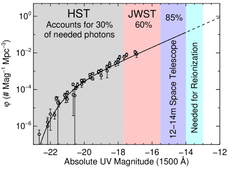
Figure 10: The reference $z=$ 7 luminosity function, highlighting the absolute magnitudes reached in deep surveys by HST, and future deep surveys by JWST and a 12-14m space telescope. Assuming that the $z=$ 7 luminosity function integrated down to M$=-$13 (with f${}_{esc}=$ 13%) can complete reionization, current HST observations only account for 30% of the needed ionizing photons. While an ultra-deep survey with JWST would only double this, a similar allocation of resources with a 12-14m class space observatory, such as HDST or ATLAST, would account for 85% of the needed photons.

8.3 Future Space-Based Telescopes

The next decade will bring the Wide-Field Infrared Survey Telescope (WFIRST), which will sport a 0.28 deg² camera housed on a 2.4m space telescope. While such a telescope will have a similar flux sensitivity as HST, the wide field will allow a number of unique investigations into the distant universe. The planned 2227 deg² High Latitude Survey (HLS) to a near-infrared depth of 26.5 AB mag will allow a truly unique view into the evolution of the bright end of the galaxy UV luminosity function at very high redshifts. When paired with optical data from the Large Synoptic Survey Telescope (LSST), this survey will enable the selection of galaxies at 4 $<z<$ 10 over this enormous area, approximately 10⁴ times the size of the CANDELS survey. WFIRST will also have a General Observer component, and as this telescope is similar in size to HST, a unique program would be to perform an extremely deep survey over a single square degree, which would encompass an area $\sim$720$\times$ that of the HUDF. While deep JWST surveys will likely provide tight constraints on the faint-end slopes at 4 $<z<$ 10 by this time, they will still be subject to significant cosmic variance uncertainties due to the small field-of-view of the JWST instruments. By probing to 29 AB mag over a very wide field, these uncertainties can be mitigated.

In Table 3 I list the expected number counts and source densities based on the reference UV luminosity functions, for both the WFIRST HLS and a hypothetical 1 deg² m${}_{\mathrm{AB}}=$ 29 WFIRST survey. At $z=$ 7, over one hundred thousand $m<$ 27 galaxies will be discovered, $>$1000$\times$ the number of bright $z=$ 7 galaxies currently known. This will allow the relatively rough constraints on the bright end of the high-redshift UV luminosity functions to be dramatically improved, allowing much more detailed investigations into the issues discussed in §5.1, such as the evolution of the impact of feedback on distant galaxies. In particular, the cosmic variance which currently plagues the bright end of the galaxy UV luminosity function (Bouwens et al. 2015c; Finkelstein et al. 2015c) will be mitigated. Combining the cosmic variance estimator of Newman & Davis (2002) for dark matter halos with the measured bias at $z=$ 7 from Barone-Nugent et al. (2014), Finkelstein et al. (2015c) found an uncertainty in the number of bright $z=$ 7 galaxies to be $\sim$20%. Using these same methods, the WFIRST HLS will have a fractional uncertainty due to cosmic variance of only 0.2%. For faint galaxies, Finkelstein et al. (2015c) found a cosmic variance uncertainty of $\sim$40%, while the analysis here shows that a deep 1 deg² survey (discovering galaxies to $m=$ 28.5) would reduce this uncertainty to only 8%. We will get a taste of this science early in the next decade, when the smaller Euclid launches, which will perform a 40 deg² deep survey $\sim$1 mag shallower than the WFIRST HLS.

Table 3: Predicted Source Counts and Densities for WFIRST HLS and Deep GO Surveys

Redshift	Limiting	N(HLS)	$n$(HLS)	N(Deep deg2)	$n$(Deep deg2)
	Magnitude		(arcmin-2)		(arcmin-2)
4	26.5	2.7 $\times$ 107	3.3	8.3 $\times$ 104	23
5	26.5	1.4 $\times$ 107	1.7	5.4 $\times$ 104	15
6	26.5	3.1 $\times$ 106	0.4	2.1 $\times$ 104	5.7
7	25.7	1.2 $\times$ 105	1.6 $\times$ 10-2	1.2 $\times$ 104	3.4
8	26.0	4.3 $\times$ 104	5.3 $\times$ 10-3	3.6 $\times$103	1.0
9	26.0	1.4 $\times$ 104	1.8 $\times$ 10-3	2.0 $\times$ 103	0.5
10	26.0	4.3 $\times$ 103	5.4 $\times$ 10-4	1.0 $\times$103	0.3

The reference luminosity functions derived in this review were used for these predictions. Columns 3 and 4 refer to the planned 2227 deg² WFIRST High Latitude Survey, while columns 5 and 6 refers to a hypothetical deep 1 deg² survey. To derive these predictions, I assumed a depth of the WFIRST HLS of 26.5 AB in the $Y$, $J$ and $H$ filters. Assuming a desired detectable Lyman break of at least 0.5 mag this implies a limiting magnitude for discoverable $z=$ 8, 9 and 10 galaxies of m${}_{\mathrm{AB}}=$ 26 for the HLS. Galaxies at $z=$ 7 will be limited by the depth of the LSST $z^{\prime}$-band, which is estimated to be 26.2, limiting $z=$ 7 galaxy studies in the WFIRST HLS to m $<$ 25.7. The bluer LSST bands will go much deeper, thus I use a limiting magnitude of 26.5 for $z=$ 4–6, such that these galaxies are still detected in the WFIRST HLS.

The somewhat more distant future (likely in the 2030s) should see the advent of a 12-14m class space telescope. Several science case and design studies are underway for concept such as the High Definition Space Telescope (HDST; Dalcanton et al. 2015) and the Advanced Technology Large Aperture Space Telescope (ATLAST; Postman et al. 2010). Such a telescope will likely be designed for the discovery of habitable worlds around other stars, but the technical requirements will result in an observatory with directly applications to the distant universe. One particular goal of such an observatory would be to account for all of the ionizing photons needed for reionization. As discussed above, the current observations likely only account for a tiny fraction of the galaxies which power reionization. As shown in Figure 10, even with a steep luminosity function, JWST deep surveys will still only account for 63% of the necessary photons. A 12-14m space telescope, reaching a limiting UV magnitude of $-$14 at $z=$ 7, will account for 85% of the total ionizing photon budget (albeit indirectly, through observations of non-ionizing UV light). More crucially, these studies will allow a direct investigation into the shape of the UV luminosity function, removing the need for the currently applied extrapolations to levels well below that which we can observe.

8.4 The Next Generation of Ground-Based Telescopes

Much as todays 8-10m class telescopes provide detailed spectroscopic followup for sources discovered by HST, the next generation of 25-40m class ground-based telescopes will allow us to study in detail the new discoveries made by JWST and future space-based telescopes. There are presently three such telescopes in development: the 25m Giant Magellan Telescope (GMT), the Thirty Meter Telescope (TMT) and the 39m European Extremely Large Telescope (E-ELT). These telescopes will be complementary in many ways. For example, the E-ELT will clearly have the largest light-gathering power, while the GMT will have the largest simultaneous field-of-view. These facilities will enable a number of new observational analyses for the $z>$ 6 universe; here I will focus on two promising future lines of inquiry directly relevant to the topics in this review.

First, high resolution spectroscopic followup of very high redshift gamma ray bursts (GRBs) offers the potential to study both galaxy ISMs and the state of the IGM at 6 $<z<$ 10. Among the most intense explosions in the universe, GRBs are predicted to occur early in the Universe’s history, and have been observed at $z=$ 8.2 (Tanvir et al. 2009) and likely at $z=$ 9.4 (Cucchiara et al. 2011), thus GRBs provide extremely bright pencil-beam flashlights into gas in the distant universe. By examining metal absorption line features in the otherwise featureless spectra of GRBs, one can directly study the abundance of heavy metals in the host galaxy of the GRB (e.g., Prochaska et al. 2007). Likewise, GRBs offer a chance to probe the ionization state and temperature of the IGM at $z>$ 7. While quasars have been utilized for these analyses previously (e.g., Fan et al. 2006), there is only a single quasar currently known at $z=$ 7, and none at higher redshifts. Should a space-based gamma ray observatory capable of discovering such sources be in place by the next decade, instruments such as GMTNIRS (Jaffe et al. 2014) available at first light on the GMT, or NIRES on the TMT and SIMPLE (Origlia et al. 2010) on the E-ELT, will allow high-resolution spectroscopic followup into the state of the ISMs of galaxies and the IGM at early times.

A second promising future analysis is the study of Ly$\alpha$ emission at $z>$ 6 to much fainter flux levels than currently possible. Current studies (primarily with MOSFIRE on Keck) can only reach low limiting Ly$\alpha$ EWs for the brightest known $z>$ 7 galaxies, rendering it presently very difficult to place constraints on Ly$\alpha$ in galaxies fainter than 27 AB mag, which comprise the majority of the known $z>$ 7 galaxy population. The 5–15$\times$ gain in light gathering power by these future telescopes will allow much deeper line flux depths to be probed. For example, deep spectroscopy on the GMT is expected to reach 5$\sigma$ limiting line fluxes of a few $\times$ 10^-19 erg s^-1 cm^-2, with the TMT and E-ELT reaching even deeper.

A direct future application of such a facility would be to map Ly$\alpha$ across both ionized and neutral regions in the 6 $<z<$ 10 universe. A future multi-object spectrograph on the GMT should have a field-of-view of $\sim$8^′, comparable to the angular size of ionized bubbles during reionization, and $>$5$\times$ larger in area than the equivalent spectrograph on JWST. While the imaging coverage needed to select galaxies over an area covering multiple such bubbles is likely beyond the realm of HST or JWST galaxy surveys, the WFIRST deep survey source densities in Table 3 show that such an instrument can simultaneously observe hundreds of 6 $<z<$ 10 galaxies down to $m=$ 28.5, allowing the use of Ly$\alpha$ emission to probe a wide range of IGM states during the epoch of reionization. This will be highly complementary with 21cm line surveys by, e.g., the Square Kilometer Array, as the combination of both surveys will allow a full picture of both the bright and dark side of reionization.

8.5 Final Words

The future is very bright for observational studies of galaxies in the first billion years after the Big Bang. As a community, we have made tremendous progress in not only discovering sources at such redshifts, but beginning to probe the physical processes dominating their evolution and gaining a better picture of how they affect the universe around them during reionization. These tantalizing glimpses into the nascent stages of our Universe leave us yearning for answers to the most pressing questions. When did the first stars form, and what were their characteristics? When did the true first galaxies form, and were their stellar populations substantially different than expected? Is reionization truly over at $z=$ 6, and was the neutral fraction substantial at $z=$ 7, or is there some other effect hindering our view of Ly$\alpha$? Finally, what is the interplay between gas and stars in such distant galaxies, and does star formation proceed differently? Although we may never truly be able to answer all of these questions, the next generation of astronomical observatories will allow us to make great progress in beginning to tease out the truth of the physics of the $z>$ 6 universe. Combining the pursuit of these studies with the new questions we will uncover with these future facilities promises to make the coming decades an extremely exciting time for observational studies of the early universe.