Material degradation due to moisture and temperature
Part 1: Mathematical model, analysis, and analytical solutions
   
Authored by

C. Xu

Graduate Student, University of Houston

M. K. Mudunuru

Graduate Student, University of Houston

K. B. Nakshatrala

Department of Civil & Environmental Engineering
University of Houston, Houston, Texas 77204–4003
phone: +1-713-743-4418, e-mail: knakshatrala@uh.edu
website: http://www.cive.uh.edu/faculty/nakshatrala

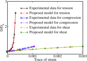
This figure shows a good agreement between the experimental data and the proposed constitutive model for the diffusivity under tension, compression and shear. Analysis is performed for various extracted sample sizes, and the coefficient of determination is found to be close to 1. This calibration study provides confidence in the proposed model to apply for brittle materials.

Abstract.

The mechanical response, serviceability, and load bearing capacity of materials and structural components can be adversely affected due to external stimuli, which include exposure to a corrosive chemical species, high temperatures, temperature fluctuations (i.e., freezing-thawing), cyclic mechanical loading, just to name a few. It is, therefore, of paramount importance in several branches of engineering – ranging from aerospace engineering, civil engineering to biomedical engineering – to have a fundamental understanding of degradation of materials, as the materials in these applications are often subjected to adverse environments. As a result of recent advancements in material science, new materials like fiber-reinforced polymers and multi-functional materials that exhibit high ductility have been developed and widely used; for example, as infrastructural materials or in medical devices (e.g., stents). The traditional small-strain approaches of modeling these materials will not be adequate. In this paper, we study degradation of materials due to an exposure to chemical species and temperature under large-strain and large-deformations. In the first part of our research work, we present a consistent mathematical model with firm thermodynamic underpinning. We then obtain semi-analytical solutions of several canonical problems to illustrate the nature of the quasi-static and unsteady behaviors of degrading hyperelastic solids.

NOMENCLATURE

$\rho$	density of solid in deformed configuration $[\mathrm{kg}\,\mathrm{m}^{-3}]$
$A$	specific Helmholtz potential $[\mathrm{J}\,\mathrm{kg}^{-1}]$
$\zeta$	dissipation functional $[\mathrm{J}\,\mathrm{kg}^{-1}\mathrm{s}^{-1}]$
$\psi$	strain energy density functional $[\mathrm{J}\,\mathrm{m}^{-3}]$
$\lambda$, $\mu$	Lamé parameters $[\mathrm{Pa}]$
$\kappa$	bulk modulus $[\mathrm{Pa}]$
$\mathbf{u}$	displacement $[\mathrm{m}]$
$\mathbf{v}$	velocity $[\mathrm{m}\,\mathrm{s}^{-1}]$
$\vartheta$	temperature $[\mathrm{K}]$
$c$	concentration $[1]$
$R_{s}$	specific vapor constant $[\mathrm{J}\,\mathrm{kg}^{-1}\mathrm{K}^{-1}]$
$c_{p}$	heat capacity $[\mathrm{J}\,\mathrm{kg}^{-1}\mathrm{K}^{-1}]$
$\mathbf{M}_{\vartheta\mathbf{E}}$	thermal expansion tensor $[\mathrm{J}\,\mathrm{m}^{-3}\mathrm{K}^{-1}]$
$\mathbf{M}_{c\mathbf{E}}$	chemical expansion tensor $[\mathrm{J}\,\mathrm{m}^{-3}]$
$d_{\vartheta c}$	thermo-chemo coupled parameter $[\mathrm{J}\,\mathrm{kg}^{-1}\mathrm{K}^{-1}]$
$\varkappa$	specific chemical potential $[\mathrm{J}\,\mathrm{kg}^{-1}]$
$\eta$	specific entropy $[\mathrm{J}\,\mathrm{kg}^{-1}\mathrm{K}^{-1}]$
$\mathbf{D}_{\vartheta\vartheta}$	thermal diffusion tensor $[\mathrm{m}^{2}\mathrm{s}^{-1}]$
$\mathbf{D}_{\varkappa\varkappa}$	diffusivity tensor $[\mathrm{m}^{2}\mathrm{s}^{-1}]$
$\mathbf{D}_{\vartheta\varkappa}$, $\mathbf{D}_{\varkappa\vartheta}$	Dufour-Soret effect tensors $[\mathrm{m}^{2}\mathrm{s}^{-1}]$
$\mathbf{T}$	Cauchy stress $[\mathrm{Pa}]$
$\mathbf{h}$	diffusive flux vector $[\mathrm{kg}\,\mathrm{m}^{-2}\mathrm{s}^{-1}]$
$\mathbf{q}$	heat flux vector $[\mathrm{J}\,\mathrm{m}^{-2}\mathrm{s}^{-1}]$
$h$	volumetric source $[\mathrm{kg}\,\mathrm{m}^{-3}\mathrm{s}^{-1}]$
$q$	volumetric heat source $[\mathrm{J}\,\mathrm{m}^{-3}\mathrm{s}^{-1}]$

1. INTRODUCTION AND MOTIVATION

Material and structural degradation is a major problem in infrastructure and various other real-life applications. Most of the well-known manifestations, such as “wear out”, “fracture”, “spalling”, and “section loss”, are related to the phenomenon of degradation [Batchelor et al., 2003]. Virtually, every material degrades when subjected to hostile environment and external stimuli. Importance of this phenomena has triggered a surge in research to develop more resistible materials. Consequently, understanding the general behavior of degrading materials has attracted the interest of researchers. A fundamental study of degradation is crucial to several branches of engineering: aerospace, mechanical, civil, and biomedical. Moreover, some new materials, such as fiber-reinforced polymers and multi-functional materials that exhibit high ductility have been widely used recently; for example, as infrastructural materials or in medical devices (e.g., stents). In order to model these materials, the traditional small-strain assumption will not be sufficient anymore.

In a nutshell, degradation means the loss in either serviceability or functionality. To be precise, a material is said to be undergoing thermal degradation at a spatial point $\mathbf{x}\in\Omega$ if the available isothermal density is lower than the reference available isothermal power at that particular point. That is,

$$\left.\frac{dA}{dt}\right|_{\vartheta>\vartheta_{\mathrm{ref}}}\leqslant\left.\frac{dA}{dt}\right|_{\vartheta=\vartheta_{\mathrm{ref}}}\ \mathrm{for}\ \mathbf{x}\in\Omega$$ (1.1)

Similarly, the chemical/moisture degradation can be defined as follows:

$$\left.\frac{dA}{dt}\right|_{c>c_{\mathrm{ref}}}\leqslant\left.\frac{dA}{dt}\right|_{c=c_{\mathrm{ref}}}\ \mathrm{for}\ \mathbf{x}\in\Omega$$ (1.2)

where $A$ denotes the specific Helmholtz potential of the material. $\Omega$ is the degrading body under consideration, $t$ is the time of interest, $\vartheta_{\mathrm{ref}}$ and $c_{\mathrm{ref}}$ are the specified reference temperature and reference concentration. Note that degradation not only reduces the durability of materials but also alters material properties. For instance, material damage can induce anisotropy in thermal conductivity and diffusivity [Peng and Landel, 1975; Venerus et al., 2004; Zheng et al., 2011].

Herein, we develop a coupled continuum mathematical model for thermal and chemical-induced degradation of solids, which are initially hyperelastic. We now outline three main reasons for such a need.

• There is irrefutable experimental evidence that many modern infrastructural materials used in repair and retrofitting applications exhibit large deformations. For example, the popular high-early-strength Engineered Cementitious Composites (ECC) are capable of delivering a compressive strength of 21 MPa within 4 hours after placement. Moreover, the long-term tensile strain capacity of ECC members is more than 2% [Li, 2006; Wang and Li, 2006].

• In order to understand degradation mechanisms due to moisture, chemical, and temperature, coupling at various levels is needed (which is due to balance laws, material parameters, boundary conditions, and initial conditions). With existing and popular multi-physics packages such ABAQUS [Aba, 2014], ANSYS [Ans, 2015], and COMSOL [Com, 2014], it is possible to couple certain degradation mechanisms to some extent at material parameters, boundary conditions, and initial conditions. However, such packages do not offer flexibility to couple important heat and mass transfer terms in balance laws. This is of utmost importance in capturing the effects of chemo-thermo-mechano degradation.

• Finally, when a new model or a thermodynamic framework is developed, stability of the solutions for the corresponding initial boundary value problem needs to be shown. However, such an analysis is rarely performed when a new degradation model/framework is developed in literature. Herein, for the proposed degradation framework we shall perform stability analysis in the sense of Lyapunov. Subsequently, this methodology shall be used to construct a robust computational framework in the part-II of the paper.

Hence, due to the above reasons small strain assumptions to model degradation and healing behavior of these infrastructural systems are rarely valid. The proposed framework takes in to account the underlying degradation mechanisms. Correspondingly, the respective parameters have a physical meaning and can be calibrated through experiments.

It should be emphasized that elasticity is an idealization. There is no material whose response is perfectly elastic. But there are situations in which the response of certain materials under normal conditions can be idealized to be hyperelastic. For example, large blood arteries and rock. Many of these materials function in hostile environments, and are constantly subjected to adverse external stimuli. One often is interested in the unsteady response of the bodies made of hyperelastic materials subjected to degradation/healing. The application areas in mind are the response of high performance cementitious materials (which undergo large strains and large deformations) and several important coupled deformation-thermal-transport processes in biomechanics and biomedicine. In the next couple of subsections, we shall discuss various degradation mechanisms and the deficiencies in the existing frameworks in modeling chemo-thermo-mechano degradation.

1.1. Degradation mechanisms

There are many mechanisms that can result in the degradation of materials and structures. In general, the degradation mechanisms can be divided into four categories: mechanical processes, chemical reactions, biological degradation [Gu et al., 1998], and radiation [Kaplan, 1989]. For mechanical processes, the performance of materials can be affected adversely by fatigue [Jung et al., 2000], pressure loading [Rajagopal et al., 2007], and swelling of solid mixtures [Buonsanti et al., 2011]. Examples of chemical degradation include humid and alkaline effects [Björk et al., 2003], exposure to chlorides and carbon-dioxide [Glasser et al., 2008], and calcium leaching [Gawin et al., 2009]. Biological degradation refers to the dissolution of materials by bacteria or other microorganisms. Degradation induced by radiation includes radiation damage as well as other mechanical and chemical processes triggered by radiation.

Table 2. Various degradation mechanics and their primary manifestation. Many other factors can be found in [Naus, 2007].

	Degradation  factor	Primary  manifestation
Physical processes	cracking	reduced  durability
	vibration	cracking
	freezing and thawing	cracking/scaling/disintegration
	abrasion/erosion/cavitation	section loss
	thermal exposure/thermal cycling	cracking/spalling/strength loss
Chemical processes	efflorescence/leaching	increased porosity
	phosphate	surface deposits
	sulfate attack	volume change/cracking
	acids/bases	disintegration/spalling/leaching
	alkali-aggregate reactions	disintegration/cracking

The coupling effects between these mechanisms can have a significant impact on the rate of deterioration of materials and structures. For instance, see Table 2 for some important factors that affect the degradation modeling in infrastructural materials such as concrete. Therefore, developing an appropriate and general model for material degradation is useful to predict the life span of a given structure. A comprehensive understanding of chemo-thermo-mechano degradation not only plays a pivotal role in improving the quality and reliability of existing infrastructure, but also has a tremendous impact on the economy [Herrmann, 2013]. In this paper, we shall assume that predominant degradation mechanisms are moisture and temperature. We propose a general three-way strongly coupled degradation model based on a thermodynamic framework. This three-way coupling is between mechanical, thermal, and transport processes.

1.2. Thermodynamics of chemo-thermo-mechano degradation

Herein, we shall provide a brief review and current status of thermal and chemical degradation. In the literature, thermal degradation is modelled based on variants of thermoelasticity by incorporating damage variables. Some popular research works in this direction are [Willam et al., 2005] for modeling thermo-mechanical damage processes in heterogeneous cementitious materials and [Allam et al., 2013] on the behavior of reinforced concrete slabs exposed to fire. On the other hand, some popular research works for the chemical degradation are [Björk et al., 2003] on the environmental effects of alkalinity and humidity on concrete slabs, [Cho and Kim, 2010] on moisture damage mechanisms occurring within asphaltic materials and pavements, [Bouadi and Sun, 1990] on thermal and moisture effects on structural stiffness and damping of laminated composites, and [Weitsman and Guo, 2002; Weitsman, 2006] on fluid-induced damage and absorption in polymeric composites. However, none of the above mentioned papers on thermal or chemical degradation have a proper thermodynamic basis.

There are two popular approaches to construct thermodynamically-consistent degradation models. The first approach is based on the theory of the internal variable, wherein a scalar (or a tensor) variable is introduced to model the degree of damage [Weitsman, 1987; Grasberger and Meschke, 2004; Springman and Bassani, 2009; Rajagopal et al., 2007]. For instance, the damage variable may represent the measure of the fraction of broken cross-links or micro-cracks in a representative volume element of the body [Kachanov, 1986; Lemaitre and Desmorat, 2005; Voyiadjis and Kattan, 2005]. The main disadvantage of this approach is that it is difficult (or sometimes impossible) to measure the internal variables through experiments or associate them to physical quantities/parameters.

The second approach is to build a thermodynamic framework by modeling all the relevant coupled processes. This achieved by taking into account the dependence of material properties on the deformation of the solid, temperature, and concentration of chemical species. The degradation parameters under this approach have physical basis and can be calibrated using experiments (for example, see Section 5 of this paper). Herein, we shall employ the second approach to develop a thermodynamically consistent degradation model. It should be noted that certain research works exist in literature wherein the degradation models using the second approach. For example, see [Muliana et al., 2009; Darbha and Rajagopal, 2009; Karra and Rajagopal, 2012; Klepach and Zohdi, 2014]. However, it appears that the above cited works suffer from the main drawback that they considered thermodynamics of chemo-thermo-mechano degradation in the context of a closed system as opposed to an open system, which is the approach taken in this paper. Moreover, the models are not as comprehensive as the one proposed in this paper.

1.3. Scope of the paper

In this paper we set out to achieve the following objectives:

1. We derive a general chemo-thermo-mechano degradation model by appealing to the maximization of rate of dissipation. It will also be shown that many popular models are special cases of the proposed mathematical model. For example, we will show that the small-strain moisture degradation model proposed in [Mudunuru and Nakshatrala, 2012] is a special case of the proposed model.

2. We will calibrate the proposed degradation model with existing experimental data sets. This calibration study should provide confidence in employing the proposed constitutive model to model degradation of various brittle and quasi-brittle materials like ceramics, glass fibers, and concrete.

3. A systematic mathematical analysis is presented for the proposed model under large/finite deformations. In particular, we shall show that the unsteady solutions under the proposed degradation model are bounded and are stable in the sense of Lyapunov.

4. Last but not the least, semi-analytical solutions to several canonical problems are presented, which provide insights into the behavior of degrading structural members. This will be valuable for developing better design and safety codes.

The rest of the paper is organized as follows. Section 2 introduces the notation, mathematical preliminaries, and the relevant balance laws. Section 3 presents a mathematical model for degradation of materials due to moisture and temperature, which is valid even under finite deformations and large strains. The constitutive relations are obtained by appealing to the maximization of rate of dissipation hypothesis, which ensures that the constitutive model satisfies the second law of thermodynamics a prior. In Section 4, the proposed model is calibrated with an experimental dataset. The coupled initial boundary value problem arising from the proposed degradation model is presented in Section 5. We also show the solutions of the proposed mathematical model are bounded and stable. In Section 6, solutions to several canonical problems are presented to illustrate the predictive capabilities of the proposed model, and to highlight the effects of degradation on the structural behavior. Finally, conclusions are drawn in Section 7.

A list of the main symbols used in the paper are provided in the Nomenclature.

2. NOTATION, PRELIMINARIES, AND BALANCE LAWS

Let us consider a body $\mathfrak{B}$. The body occupies a reference configuration $\Omega_{0}(\mathfrak{B})\subset\mathbb{R}^{nd}$, where “$nd$” denotes the number of spatial dimensions. A point in the reference configuration is denoted by $\mathbf{p}\in\Omega_{0}(\mathfrak{B})$. We shall denote the time by $t\in[0,\mathcal{T}]$, where $\mathcal{T}$ is the length of the time interval of interest. Due to motion, the body occupies different spatial configurations with time. We shall denote the configuration occupied by the body at time $t$ as $\Omega_{t}(\mathfrak{B})\subset\mathbb{R}^{nd}$. A corresponding spatial point will be denoted as $\mathbf{x}\in\Omega_{t}(\mathfrak{B})$. The gradient and divergence operators with respect to $\mathbf{p}$ are, respectively, denoted by $\mathrm{Grad}[\bullet]$ and $\mathrm{Div}[\bullet]$. Similarly, the gradient and divergence operators with respect to $\mathbf{x}$ are, respectively, denoted by $\mathrm{grad}[\bullet]$ and $\mathrm{div}[\bullet]$.

The motion of the body is mathematically described by the following invertible mapping:

$$\mathbf{x}=\boldsymbol{\varphi}(\mathbf{p},t)$$ (2.1)

The displacement vector field can then be written as:

$$\mathbf{u}=\mathbf{x}-\mathbf{p}=\boldsymbol{\varphi}(\mathbf{p},t)-\mathbf{p}$$ (2.2)

The velocity vector field is defined as:

$$\mathbf{v}=\dot{\mathbf{x}}:=\frac{\partial\boldsymbol{\varphi}(\mathbf{p},t)}{\partial t}$$ (2.3)

where a superposed dot indicates the material/total time derivative, which is the derivative with respect to time holding the reference coordinates fixed. The gradient of motion (which is also referred to as the deformation gradient) is defined as:

$$\mathbf{F}=\mathrm{Grad}[\mathbf{x}]\equiv\frac{\partial\boldsymbol{\varphi}(\mathbf{p},t)}{\partial\mathbf{p}}=\mathbf{I}+\mathrm{Grad}[\mathbf{u}]$$ (2.4)

where $\mathbf{I}$ denotes the second-order identity tensor. The corresponding right Cauchy-Green tensor is denoted by:

$$\mathbf{C}=\mathbf{F}^{\mathrm{T}}\mathbf{F}$$ (2.5)

where $(\bullet)^{\mathrm{T}}$ denotes the transpose of a second-order tensor. The velocity gradient with respect to $\mathbf{x}$ and the symmetric part of the velocity gradient are, respectively, defined as follows:

$$\mathbf{L} :=\mathrm{grad}[\mathbf{v}]\equiv\dot{\mathbf{F}}\mathbf{F}^{-1}$$ (2.6)

$$\mathbf{D} :=\frac{1}{2}\left(\mathbf{L}+\mathbf{L}^{\mathrm{T}}\right)$$ (2.7)

The Green-St. Venant strain tensor is defined as:

$$\mathbf{E}=\frac{1}{2}(\mathbf{C}-\mathbf{I})=\frac{1}{2}\left(\mathrm{Grad}[\mathbf{u}]+\mathrm{Grad}[\mathbf{u}]^{\mathrm{T}}+\mathrm{Grad}[\mathbf{u}]^{\mathrm{T}}\mathrm{Grad}[\mathbf{u}]\right)$$ (2.8)

In situations the following assumption holds:

$$\mathop{\mathrm{max}}_{\mathbf{p}\in\Omega_{0}(\mathfrak{B}),t\in[0,\mathcal{T}]}\sqrt{\|\boldsymbol{\varphi}(\mathbf{p},t)-\mathbf{p}\|^{2}+\|\mathrm{Grad}[\mathbf{u}]\|^{2}}\ll 1$$ (2.9)

one is justified to employ the following linearized strain tensor:

$$\mathbf{E}_{l}=\frac{1}{2}\left(\mathrm{Grad}[\mathbf{u}]+\mathrm{Grad}[\mathbf{u}]^{\mathrm{T}}\right)\approx\frac{1}{2}\left(\mathrm{grad}[\mathbf{u}]+\mathrm{grad}[\mathbf{u}]^{\mathrm{T}}\right)$$ (2.10)

where $\|\bullet\|$ denotes the Frobenius norm [Antman, 1995].

Since we will be dealing with processes in addition to the mechanical deformation, we need to introduce quantities other than the ones that are associated with the kinematics. We will denote the temperature by $\vartheta$ and the specific entropy by $\eta$. The mass fraction of the chemical species is denoted by $c$ and the corresponding chemical potential is denoted by $\varkappa$. The temperature, mass fraction of chemical species, entropy, and chemical potential are all scalar fields, while the displacement, velocity, and acceleration are vector fields. In some situations, it may be needed to explicitly indicate the functional dependence of these quantities. We employ a standard notation, which will be illustrated through the temperature field. The temperature in terms of reference coordinates and spatial coordinates will be denoted as follows:

$$\vartheta=\tilde{\vartheta}(\mathbf{p},t)=\hat{\vartheta}(\mathbf{x},t)$$ (2.11)

2.1. Balance laws

For our study, we shall consider the thermodynamic system to be the entire degrading body. Moreover, we shall assume this thermodynamic system to be an open system. That is, heat and mass transfers can occur across the boundary of the system. We now present the balance laws that govern the evolution of the chosen system.

The balance of mass of the solid in the degrading body takes the following form:

$$\dot{\rho}+\rho\,\mathrm{div}[\mathbf{v}]=0$$ (2.12)

where $\rho$ is the density of the solid in the deformed configuration $\Omega_{t}(\mathfrak{B})$. The balance of a chemical species, which is being transported in the degrading body, can be mathematically written as:

$$\rho\dot{c}+\mathrm{div}[\mathbf{h}]=h$$ (2.13)

where $\mathbf{h}$ is the mass transfer flux vector in the deformed configuration, and $h$ is the volumetric source of the chemical species in the deformed configuration. We assume that the chemical species cannot take partial stresses, which is a reasonable assumption in the degradation of materials due to small concentrations of moisture. One can handle large moisture contents by introducing partial stresses and using the theory of interacting continua (which is often referred to mixture theory) [Bowen, 1976]. We do not address such issues, as our focus is degradation due to small concentrations of moisture or chemicals. The balance of linear momentum of the solid can be written as:

$$\rho\dot{\mathbf{v}}=\mathrm{div}[\mathbf{T}]+\rho\mathbf{b}$$ (2.14)

where $\mathbf{b}$ is the specific body force, and $\mathbf{T}$ is the Cauchy stress in the solid. Assuming that there is no internal couples, the balance of angular momentum of the solid reads:

$$\mathbf{T}=\mathbf{T}^{\mathrm{T}}$$ (2.15)

Assuming that the balance of linear momentum (i.e., equation (2.14)) holds, the balance of energy of the system (i.e., the first law of thermodynamics) can be written as:

$$\rho\frac{\mathrm{d}}{\mathrm{d}t}\left(A+\vartheta\eta\right)=\mathbf{T}\bullet\mathbf{D}-\mathrm{div}[\varkappa\mathbf{h}]+\varkappa h-\mathrm{div}[\mathbf{q}]+q$$ (2.16)

where ${A}$ is the specific Helmholtz potential, $\mathbf{q}$ is the heat flux vector in the deformed configuration, and $q$ is the volumetric heat source in the deformed configuration. In our study, we assume that the Helmholtz potential $A$ to depend on $\mathbf{F}$, $c$, and $\vartheta$. We also have the following relations for the chemical potential and specific entropy:

$$\varkappa :=+\frac{\partial A}{\partial c}$$ (2.17)

$$\eta :=-\frac{\partial A}{\partial\vartheta}$$ (2.18)

Assuming the balance of chemical species to hold, we then have the following convenient form for the balance of energy:

$$\rho\left(\frac{\partial A}{\partial\mathbf{F}}\mathbf{F}^{\mathrm{T}}\bullet\mathbf{D}+\vartheta\dot{\eta}\right)=\mathbf{T}\bullet\mathbf{D}-\mathrm{div}[\mathbf{q}]-\mathrm{grad}[\varkappa]\bullet\mathbf{h}+q$$ (2.19)

The localized version of the second law of thermodynamics in the deformed configuration (by assuming that all the aforementioned balance laws to hold) takes the following form:

$$\rho\left(\frac{\partial A}{\partial\mathbf{F}}\mathbf{F}^{\mathrm{T}}\bullet\mathbf{D}\right)=\mathbf{T}\bullet\mathbf{D}-\frac{1}{\vartheta}\mathrm{grad}[\vartheta]\bullet\mathbf{q}-\mathrm{grad}[\varkappa]\bullet\mathbf{h}-\rho\zeta$$ (2.20)

where $\zeta$ is the specific rate of dissipation functional, which is non-negative. The above equation is a stronger version than the second law of thermodynamics, which is a global law and not a local one. The second law of thermodynamics does not assert that the rate of entropy production be non-decreasing at each and every point in the system/body. Strictly speaking, equation (2.20) should be referred to as the reduced local dissipation equality. Another point to highlight is that the second law of thermodynamics, in its original form, is in the form of an inequality. The introduction of the non-negative dissipation functional, which acts as a slack variable, converts the inequality into an equality, as provided in equation (2.20).

2.2. The maximization of rate of dissipation

Among the various methodologies to derive constitutive relations (e.g., see [Maugin, 1998]), the axiom of maximization of rate of dissipation put-forth by Ziegler [Ziegler, 1983] is an attractive procedure. Herein, we extend this procedure to the open thermodynamic system under consideration. We obtain the constitutive relations using the maximization of rate of dissipation hypothesis, which needs the prescription of two functionals – the Helmholtz potential and the dissipation functional. We assume the functional dependence of the Helmholtz potential and the dissipation functional to be $\hat{A}(\mathbf{F},c,\vartheta)$ and $\hat{\zeta}(\mathbf{D},\mathrm{grad}[\vartheta],\mathrm{grad}[\varkappa];\mathbf{F},\vartheta,c)$.

The mathematical statement of maximization of rate of dissipation can be written as follows:

$$\mathop{\mathrm{maximize}}\limits_{\mathbf{D},\mathrm{grad}[\vartheta],\mathrm{grad}[\varkappa]}\;\; \rho\zeta=\rho\hat{\zeta}(\mathbf{D},\mathrm{grad}[\vartheta],\mathrm{grad}[\varkappa];\mathbf{F},\vartheta,c)$$ (2.21a)

$$\mathrm{subject\ to}\ \rho\left(\frac{\partial A}{\partial\mathbf{F}}\mathbf{F}^{\mathrm{T}}\bullet\mathbf{D}\right)=\mathbf{T}\bullet\mathbf{D}-\frac{1}{\vartheta}\mathrm{grad}[\vartheta]\bullet\mathbf{q}-\mathrm{grad}[\varkappa]\bullet\mathbf{h}-\rho\zeta$$ (2.21b)

Note that $\rho\zeta$ is maximized with respect to arguments to the left side of ‘;’. Using the method of Lagrange multipliers, the above constrained optimization problem is equivalent to the following unconstrained optimization problem:

$$\mathop{\mathrm{extremize}}\limits_{\mathbf{D},\mathrm{grad}[\vartheta],\mathrm{grad}[\varkappa],\Lambda_{t}}\;\; \rho\hat{\zeta}(\mathbf{D},\mathrm{grad}[\vartheta],\mathrm{grad}[\varkappa];\mathbf{F},\vartheta,c)$$

$$+\, \Lambda_{t}\left(\rho\left(\frac{\partial A}{\partial\mathbf{F}}\mathbf{F}^{\mathrm{T}}\bullet\mathbf{D}\right)-\mathbf{T}\bullet\mathbf{D}+\frac{1}{\vartheta}\mathrm{grad}[\vartheta]\bullet\mathbf{q}+\mathrm{grad}[\varkappa]\bullet\mathbf{h}+\rho\zeta\right)$$ (2.22)

where $\Lambda_{t}$ is the Lagrange multiplier enforcing the constraint (2.21b). The first-order optimal conditions give rise to the following relations:

$$\mathbf{T}=\rho\frac{\partial A}{\partial\mathbf{F}}\mathbf{F}^{\mathrm{T}}+\left(\frac{1+\Lambda_{t}}{\Lambda_{t}}\right)\rho\frac{\partial\zeta}{\partial\mathbf{D}}$$ (2.23a)

$$\frac{1}{\vartheta}\mathbf{q}=-\left(\frac{1+\Lambda_{t}}{\Lambda_{t}}\right)\rho\frac{\partial\zeta}{\partial\mathrm{grad}[\vartheta]}$$ (2.23b)

$$\mathbf{h}=-\left(\frac{1+\Lambda_{t}}{\Lambda_{t}}\right)\rho\frac{\partial\zeta}{\partial\mathrm{grad}[\varkappa]}$$ (2.23c)

$$\rho\left(\frac{\partial A}{\partial\mathbf{F}}\mathbf{F}^{\mathrm{T}}\bullet\mathbf{D}\right)-\mathbf{T}\bullet\mathbf{D}+\frac{1}{\vartheta}\mathrm{grad}[\vartheta]\bullet\mathbf{q}+\mathrm{grad}[\varkappa]\bullet\mathbf{h}+\rho\zeta=0$$ (2.23d)

The above equations can be obtained by taking (Gâteaux) variation of the objective function in equation (2.2) with respect to $\mathbf{D}$, $\mathrm{grad}[\vartheta]$, $\mathrm{grad}[\varkappa]$ and $\Lambda_{t}$, respectively. By straightforward manipulations on equations (2.23a)–(2.23d), the Lagrange multiplier $\Lambda_{t}$ can be explicitly calculated as follows:

$$\Lambda_{t}=\left[\frac{\zeta}{\frac{\partial\zeta}{\partial\mathbf{D}}\bullet\mathbf{D}+\frac{\partial\zeta}{\partial\mathrm{grad}[\vartheta]}\bullet\mathrm{grad}[\vartheta]+\frac{\partial\zeta}{\partial\mathrm{grad}[\varkappa]}\bullet\mathrm{grad}[\varkappa]}-1\right]^{-1}$$ (2.24)

If the rate of dissipation functional $\zeta$ is a homogeneous functional of order 2 with respect to $\mathbf{D}$, $\mathrm{grad}[\vartheta]$ and $\mathrm{grad}[\varkappa]$, we then have

$$\frac{\partial\zeta}{\partial\mathbf{D}}\bullet\mathbf{D}+\frac{\partial\zeta}{\partial\mathrm{grad}[\vartheta]}\bullet\mathrm{grad}[\vartheta]+\frac{\partial\zeta}{\partial\mathrm{grad}[\varkappa]}\bullet\mathrm{grad}[\varkappa]=2\zeta$$ (2.25)

which further implies that $\Lambda_{t}=-2$. The constitutive relations under $\Lambda_{t}=-2$ will simplify to:

$$\mathbf{T}=\rho\frac{\partial A}{\partial\mathbf{F}}\mathbf{F}^{\mathrm{T}}+\frac{1}{2}\rho\frac{\partial\zeta}{\partial\mathbf{D}}$$ (2.26a)

$$\mathbf{q}=-\frac{\vartheta}{2}\rho\frac{\partial\zeta}{\partial\mathrm{grad}[\vartheta]}$$ (2.26b)

$$\mathbf{h}=-\frac{1}{2}\rho\frac{\partial\zeta}{\partial\mathrm{grad}[\varkappa]}$$ (2.26c)

Remark 2.1.

It should be emphasized that the dissipation functional need not be a homogeneous functional of order two in terms of $\mathbf{F}$, $c$ and $\vartheta$. The maximization of the rate of dissipation certainly does not require such an assumption. However, we shall make such an assumption, as it is convenient and the resulting constitutive relations can still model the desired degradation mechanisms.

2.3. Governing equations in the reference configuration

Since we are also interested in developing a computational framework and obtaining numerical solutions, it will be convenient to write the balance laws in the reference configuration. To this end, we introduce:

$$J\equiv\mathrm{det}[\mathbf{F}]$$ (2.27)

where $\mathrm{det}[\bullet]$ denotes the determinant. The balance of mass in the reference configuration can be written as:

$$\rho_{0}=J\rho$$ (2.28)

where $\rho_{0}$ is the density of the undeformed solid. The balance of chemical species in the reference configuration can be rewritten as:

$$\rho_{0}\dot{c}+\mathrm{Div}[\mathbf{h}_{0}]=h_{0}$$ (2.29)

where $\mathbf{h}_{0}=J\mathbf{F}^{-1}\mathbf{h}$ is the diffusive flux vector in the reference configuration and $h_{0}=Jh$ is the volumetric source in the reference configuration. The balance of linear momentum in the reference configuration takes the following form:

$$\rho_{0}\dot{\mathbf{v}}=\mathrm{Div}[\mathbf{P}]+\rho_{0}\mathbf{b}$$ (2.30)

where $\mathbf{P}=J\mathbf{T}\mathbf{F}^{-\mathrm{T}}$ is the first Piola-Kirchhoff stress. The balance of angular momentum in the reference configuration takes the following form:

$$\mathbf{P}\mathbf{F}^{\mathrm{T}}=\mathbf{F}\mathbf{P}^{\mathrm{T}}$$ (2.31)

In the reference configuration, the balance of energy can be written as:

$$\rho_{0}\left(\frac{\partial A}{\partial\mathbf{F}}\bullet\dot{\mathbf{F}}+\vartheta\dot{\eta}\right)=\mathbf{P}\bullet\dot{\mathbf{F}}-\mathrm{Div}[\mathbf{q}_{0}]-\mathrm{Grad}[\varkappa]\bullet\mathbf{h}_{0}+q_{0}$$ (2.32)

where $\mathbf{q}_{0}=J\mathbf{F}^{-1}\mathbf{q}$ is the heat flux vector in the reference configuration and $q_{0}=Jq$ is the volumetric heat source in the reference configuration. In the reference configuration, the second law can be rewritten as:

$$\rho_{0}\left(\frac{\partial A}{\partial\mathbf{F}}\bullet\dot{\mathbf{F}}\right)=\mathbf{P}\bullet\dot{\mathbf{F}}-\frac{1}{\vartheta}\mathrm{Grad}[\vartheta]\bullet\mathbf{q}_{0}-\mathrm{Grad}[\varkappa]\bullet\mathbf{h}_{0}-\rho_{0}\zeta_{0}$$ (2.33)

where $\zeta_{0}=\zeta$ is the non-negative rate of dissipation functional in the reference configuration.

2.3.1. Maximization of rate of dissipation in the reference configuration

The mathematical statement of maximization of rate of dissipation can be written as follows:

$$\mathop{\mathrm{maximize}}\limits_{\dot{\mathbf{F}},\mathrm{Grad}[\vartheta],\mathrm{Grad}[\varkappa]}\;\; \rho_{0}\zeta_{0}=\rho_{0}\tilde{\zeta}(\dot{\mathbf{F}},\mathrm{Grad}[\vartheta],\mathrm{Grad}[\varkappa];\mathbf{F},\vartheta,c)$$ (2.34a)

$$\mathrm{subject\ to}\ \rho_{0}\left(\frac{\partial A}{\partial\mathbf{F}}\bullet\dot{\mathbf{F}}\right)=\mathbf{P}\bullet\dot{\mathbf{F}}-\frac{1}{\vartheta}\mathrm{Grad}[\vartheta]\bullet\mathbf{q}_{0}-\mathrm{Grad}[\varkappa]\bullet\mathbf{h}_{0}-\rho_{0}\zeta_{0}$$ (2.34b)

Using the method of Lagrange multipliers, one can obtain the following equivalent unconstrained optimization problem:

$$\mathop{\mathrm{extremize}}\limits_{\dot{\mathbf{F}},\mathrm{Grad}[\vartheta],\mathrm{Grad}[\varkappa],\Lambda_{0}}\;\; \rho_{0}\tilde{\zeta}(\dot{\mathbf{F}},\mathrm{Grad}[\vartheta],\mathrm{Grad}[\varkappa];\mathbf{F},\vartheta,c)$$

$$+\, \Lambda_{0}\left(\rho_{0}\left(\frac{\partial A}{\partial\mathbf{F}}\bullet\dot{\mathbf{F}}\right)-\mathbf{P}\bullet\dot{\mathbf{F}}+\frac{1}{\vartheta}\mathrm{Grad}[\vartheta]\bullet\mathbf{q}_{0}+\mathrm{Grad}[\varkappa]\bullet\mathbf{h}_{0}+\rho_{0}\zeta_{0}\right)$$ (2.35)

where $\Lambda_{0}$ is the Lagrange multiplier enforcing the constraint given by equation (2.34b). The first-order optimality conditions give rise to the following constitutive relations:

$$\mathbf{P}=\rho_{0}\frac{\partial A}{\partial\mathbf{F}}+\left(\frac{1+\Lambda_{0}}{\Lambda_{0}}\right)\rho_{0}\frac{\partial\zeta_{0}}{\partial\dot{\mathbf{F}}}$$ (2.36a)

$$\frac{1}{\vartheta}\mathbf{q}_{0}=-\left(\frac{1+\Lambda_{0}}{\Lambda_{0}}\right)\rho_{0}\frac{\partial\zeta_{0}}{\partial\mathrm{Grad}[\vartheta]}$$ (2.36b)

$$\mathbf{h}_{0}=-\left(\frac{1+\Lambda_{0}}{\Lambda_{0}}\right)\rho_{0}\frac{\partial\zeta_{0}}{\partial\mathrm{Grad}[\varkappa]}$$ (2.36c)

$$\rho_{0}\left(\frac{\partial A}{\partial\mathbf{F}}\bullet\dot{\mathbf{F}}\right)-\mathbf{P}\bullet\dot{\mathbf{F}}+\frac{1}{\vartheta}\mathrm{Grad}[\vartheta]\bullet\mathbf{q}_{0}+\mathrm{Grad}[\varkappa]\bullet\mathbf{h}_{0}+\rho_{0}\zeta_{0}=0$$ (2.36d)

Similar to the derivation presented earlier in the context of current configuration, the Lagrange multiplier $\Lambda_{0}$ can be explicitly calculated as follows:

$$\Lambda_{0}=\left[\frac{\zeta_{0}}{\frac{\partial\zeta_{0}}{\partial\dot{\mathbf{F}}}\bullet\dot{\mathbf{F}}+\frac{\partial\zeta_{0}}{\partial\mathrm{Grad}[\vartheta]}\bullet\mathrm{Grad}[\vartheta]+\frac{\partial\zeta_{0}}{\partial\mathrm{Grad}[\varkappa]}\bullet\mathrm{Grad}[\varkappa]}-1\right]^{-1}$$ (2.37)

If the rate of dissipation functional in the reference configuration $\zeta_{0}$ is a homogeneous functional of order 2, we have

$$\frac{\partial\zeta_{0}}{\partial\dot{\mathbf{F}}}\bullet\dot{\mathbf{F}}+\frac{\partial\zeta_{0}}{\partial\mathrm{Grad}[\vartheta]}\bullet\mathrm{Grad}[\vartheta]+\frac{\partial\zeta_{0}}{\partial\mathrm{Grad}[\varkappa]}\bullet\mathrm{Grad}[\varkappa]=2\zeta_{0}$$ (2.38)

which further implies that $\Lambda_{0}=-2$. The constitutive relations under $\Lambda_{0}=-2$ take the following form:

$$\mathbf{P}=\rho_{0}\frac{\partial A}{\partial\mathbf{F}}+\frac{1}{2}\rho_{0}\frac{\partial\zeta_{0}}{\partial\dot{\mathbf{F}}}$$ (2.39a)

$$\mathbf{q}_{0}=-\frac{\vartheta}{2}\rho_{0}\frac{\partial\zeta_{0}}{\partial\mathrm{Grad}[\vartheta]}$$ (2.39b)

$$\mathbf{h}_{0}=-\frac{1}{2}\rho_{0}\frac{\partial\zeta_{0}}{\partial\mathrm{Grad}[\varkappa]}$$ (2.39c)

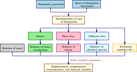
The overarching idea behind the proposed chemo-thermo-mechano degradation model is shown in Figure 1. In the next section, we will develop the proposed constitutive model by appealing to the maximization of rate of dissipation. Solving the coupled balance laws (even including the evolution equation for internal variable), we can get the displacement, temperature, and concentration (internal variable, if needed).

Figure 1. Overarching idea of the proposed degradation framework: This flowchart shows the overarching idea behind the proposed framework. We shall appeal to the axiom of maximization of rate of dissipation to obtain constitutive relations for stress, heat flux, diffusion flux, and evolution equation for internal variable (if required). Solving the coupled equations, we get the solution for displacement, temperature, concentration, and internal variable (if required).

3. A GENERAL CONSTITUTIVE MODEL FOR CHEMO-THERMO-MECHANO DEGRADATION

Under the maximization of rate of dissipation hypothesis, the constitutive relations can be obtained by prescribing two functionals – the Helmholtz potential and the dissipation functional. Philosophically, the Helmholtz potential quantifies the way in which the material stores energy, whereas the dissipation functional quantifies the way in which the material dissipates energy. For our proposed chemo-thermo-mechano degradation model, we prescribe the following functional forms for the specific Helmholtz potential and the rate of dissipation functional:

$$A=\hat{A}(\mathbf{F},c,\vartheta) =\frac{1}{\rho_{0}}\psi-\frac{1}{2}\frac{c_{p}}{\vartheta_{\mathrm{ref}}}\left\{\vartheta-\vartheta_{\mathrm{ref}}\right\}^{2}-\frac{1}{\rho_{0}}\left\{\vartheta-\vartheta_{\mathrm{ref}}\right\}\mathbf{M}_{\vartheta\mathbf{E}}\bullet\mathbf{E}+d_{\vartheta c}\left\{\vartheta-\vartheta_{\mathrm{ref}}\right\}\left\{c-c_{\mathrm{ref}}\right\}$$

$$-\frac{1}{\rho_{0}}\left\{c-c_{\mathrm{ref}}\right\}\mathbf{M}_{c\mathbf{E}}\bullet\mathbf{E}+\frac{R_{s}\vartheta_{\mathrm{ref}}}{2}\{c-c_{\mathrm{ref}}\}^{2}$$ (3.1)

$$\zeta=\hat{\zeta}(\mathbf{D},\mathrm{grad}[\vartheta],\mathrm{grad}[\varkappa];\mathbf{F},\vartheta,c) =\frac{c_{p}}{\vartheta}\mathrm{grad}[\vartheta]\bullet\mathbf{D}_{\vartheta\vartheta}\mathrm{grad}[\vartheta]+\frac{1}{\vartheta}\mathrm{grad}[\vartheta]\bullet\mathbf{D}_{\vartheta\varkappa}\mathrm{grad}[\varkappa]$$

$$+\frac{1}{\vartheta}\mathrm{grad}[\varkappa]\bullet\mathbf{D}_{\varkappa\vartheta}\mathrm{grad}[\vartheta]+\frac{1}{R_{s}\vartheta_{\mathrm{ref}}}\mathrm{grad}[\varkappa]\bullet\mathbf{D}_{\varkappa\varkappa}\mathrm{grad}[\varkappa]$$ (3.2)

where $R_{s}=R/M$. $R_{s}$ and $R$ denote the specific vapor constant and the universal vapor constant respectively, $M$ is the molecular mass of chemical species. $\vartheta_{\mathrm{ref}}$ and $c_{\mathrm{ref}}$ are the specified reference temperature and reference mass concentration, which depend on the underlying boundary value problem. We denote $c_{p}$ as the coefficient of heat capacity, $d_{\vartheta c}$ as the thermo-chemo coupled parameter [Sih et al., 1986], $\mathbf{M}_{\vartheta\mathbf{E}}$ as the anisotropic coefficient of thermal expansion (which is assumed to be independent of temperature, concentration, and strain), and $\mathbf{M}_{c\mathbf{E}}$ as the anisotropic coefficient of chemical expansion due to concentration (which is also assumed to be independent of temperature, concentration, and strain). Both $\mathbf{M}_{\vartheta\mathbf{E}}$ and $\mathbf{M}_{c\mathbf{E}}$ are assumed to be symmetric. $\mathbf{D}_{\vartheta\vartheta}$ is the anisotropic thermal conductivity tensor and $\mathbf{D}_{\varkappa\varkappa}$ is the anisotropic diffusivity tensor. $\mathbf{D}_{\vartheta\varkappa}$ corresponds to the anisotropic Soret effect tensor, which characterizes the transport of chemical species caused by temperature gradient. Similarly, $\mathbf{D}_{\varkappa\vartheta}$ is the Dufour effect tensor, which represents the heat flow caused by a concentration gradient.

Remark 3.1.

In chemo-thermo-elasticity and in modeling degradation of materials due to transport and reaction of chemical species, coefficient of chemical expansion $\mathbf{M}_{c\mathbf{E}}$ and thermo-chemo coupling parameter $d_{\vartheta c}$ play a vital role (see [Sih et al., 1986, Chapter-5] and references therein). Induced-strains due to chemical expansivity will be significant in harsh environmental conditions and cannot be neglected [Sih et al., 1986]. Considerable inquest has been made in literature to experimentally measure $\mathbf{M}_{c\mathbf{E}}$ in ceramics [Adler, 2001; Morozovska et al., 2011; Blond and Richet, 2008], laminated and polymer composites [Sih et al., 1986; Bouadi and Sun, 1989; Cai and Weitsman, 1994], elastomers and biological materials [Harper, 2002; Myers et al., 1984; Lai et al., 1991], and concrete structures [Ulm et al., 2000; Černy and Rovnaníková, 2002; Swamy, 2002]. However, adequate progress has not been made yet to develop constitutive models and computational frameworks for such chemo-thermo-elastic materials or materials undergoing chemical-induced degradation. Herein, we shall take a step forward to address this issue.

Remark 3.2.

It should be noted that in the absence of electrical and magnetic fields, all of the above tensors are symmetric [Bowen, 1976; Coussy, 2004; Jarkova et al., 2001]. Moreover, from the Onsager reciprocal relations (which was put-forth by Onsager in 1930s [Onsager, 1931a, b]) we have the following relationship between the Soret effect tensor and the Dufour effect tensor.

$$\mathbf{D}_{\vartheta\varkappa}=\mathbf{D}_{\varkappa\vartheta}$$ (3.3)

Additionally, physics demands that the tensors $\mathbf{D}_{\vartheta\vartheta}$ and $\mathbf{D}_{\varkappa\varkappa}$ are positive definite.

Remark 3.3.

Note that the specific Helmholtz potential and correspondingly the dissipation functional for diffusion can also be modelled using the following expressions:

$$A_{c} =R_{s}\vartheta_{\mathrm{ref}}c\{\mathrm{ln}[c]-1\}$$ (3.4)

$$\zeta_{c} =\frac{c}{R_{s}\vartheta_{\mathrm{ref}}}\mathrm{grad}[\varkappa]\bullet\mathbf{D}_{\varkappa\varkappa}\mathrm{grad}[\varkappa]$$ (3.5)

Both equations (3)–(3) and (3.4)–(3.5) result in similar partial differential equation structure for modeling Fickian diffusion.

Under the proposed model, the specific entropy and chemical potential take the following form:

$$\eta=-\frac{\partial A}{\partial\vartheta}=-\frac{1}{\rho_{0}}\frac{\partial\psi}{\partial\vartheta}+\frac{c_{p}}{\vartheta_{\mathrm{ref}}}\{\vartheta-\vartheta_{\mathrm{ref}}\}+\frac{1}{\rho_{0}}\mathbf{M}_{\vartheta\mathbf{E}}\bullet\mathbf{E}-d_{\vartheta c}\{c-c_{\mathrm{ref}}\}$$ (3.6)

$$\varkappa=\frac{\partial A}{\partial c}=\frac{1}{\rho_{0}}\frac{\partial\psi}{\partial c}+R_{s}\vartheta_{\mathrm{ref}}\{c-c_{\mathrm{ref}}\}-\frac{1}{\rho_{0}}\mathbf{M}_{c\mathbf{E}}\bullet\mathbf{E}+d_{\vartheta c}\{\vartheta-\vartheta_{\mathrm{ref}}\}$$ (3.7)

From equations (2.26a)–(2.26c), we have the constitutive relations in deformed configuration as:

$$\mathbf{T}=\rho\frac{\partial A}{\partial\mathbf{F}}\mathbf{F}^{\mathrm{T}}=\frac{1}{J}\frac{\partial\psi}{\partial\mathbf{F}}\mathbf{F}^{\mathrm{T}}-\frac{1}{J}\left\{\vartheta-\vartheta_{\mathrm{ref}}\right\}\mathbf{F}\mathbf{M}_{\vartheta\mathbf{E}}\mathbf{F}^{\mathrm{T}}-\frac{1}{J}\left\{c-c_{\mathrm{ref}}\right\}\mathbf{F}\mathbf{M}_{c\mathbf{E}}\mathbf{F}^{\mathrm{T}}$$ (3.8a)

$$\mathbf{q}=-\frac{\vartheta}{2}\rho\frac{\partial\hat{\zeta}}{\partial\mathrm{grad}[\vartheta]}=-\rho c_{p}\mathbf{D}_{\vartheta\vartheta}\mathrm{grad}[\vartheta]-\frac{\rho}{2}\mathbf{D}_{\vartheta\varkappa}\mathrm{grad}[\varkappa]-\frac{\rho}{2}\mathbf{D}_{\varkappa\vartheta}\mathrm{grad}[\varkappa]$$ (3.8b)

$$\mathbf{h}=-\frac{1}{2}\rho\frac{\partial\hat{\zeta}}{\partial\mathrm{grad}[\varkappa]}=-\frac{\rho}{R_{s}\vartheta_{\mathrm{ref}}}\mathbf{D}_{\varkappa\varkappa}\mathrm{grad}[\varkappa]-\frac{\rho}{2\vartheta}\mathbf{D}_{\vartheta\varkappa}\mathrm{grad}[\vartheta]-\frac{\rho}{2\vartheta}\mathbf{D}_{\varkappa\vartheta}\mathrm{grad}[\vartheta]$$ (3.8c)

The rate of dissipation functional for the degradation model in the reference configuration is taken as follows:

$$\zeta =\tilde{\zeta}(\dot{\mathbf{F}},\mathrm{Grad}[\vartheta],\mathrm{Grad}[\varkappa];\mathbf{F},\vartheta,c)$$

$$=\frac{c_{p}}{\vartheta}\mathrm{Grad}[\vartheta]\bullet\overline{\mathbf{D}}_{\vartheta\vartheta}\mathrm{Grad}[\vartheta]+\frac{1}{\vartheta}\mathrm{Grad}[\vartheta]\bullet\overline{\mathbf{D}}_{\vartheta\varkappa}\mathrm{Grad}[\varkappa]$$

$$+\frac{1}{\vartheta}\mathrm{Grad}[\varkappa]\bullet\overline{\mathbf{D}}_{\varkappa\vartheta}\mathrm{Grad}[\vartheta]+\frac{1}{R_{s}\vartheta_{\mathrm{ref}}}\mathrm{Grad}[\varkappa]\bullet\overline{\mathbf{D}}_{\varkappa\varkappa}\mathrm{Grad}[\varkappa]$$ (3.9)

where $\overline{\mathbf{D}}_{\alpha\beta}=\mathbf{F}^{-1}\mathbf{D}_{\alpha\beta}\mathbf{F}^{-T}$, $\alpha$ and $\beta$ represent $\vartheta$ or $\varkappa$. Correspondingly, the constitutive relations in the reference configuration take the following form:

$$\mathbf{P} =\rho_{0}\frac{\partial A}{\partial\mathbf{F}}=\frac{\partial\psi}{\partial\mathbf{F}}-\left\{\vartheta-\vartheta_{\mathrm{ref}}\right\}\mathbf{F}\mathbf{M}_{\vartheta\mathbf{E}}-\left\{c-c_{\mathrm{ref}}\right\}\mathbf{F}\mathbf{M}_{c\mathbf{E}}$$ (3.10a)

$$\mathbf{q}_{0} =-\frac{\vartheta}{2}\rho_{0}\frac{\partial\tilde{\zeta}}{\partial\mathrm{Grad}[\vartheta]}=-\rho_{0}c_{p}\overline{\mathbf{D}}_{\vartheta\vartheta}\mathrm{Grad}[\vartheta]-\frac{\rho_{0}}{2}\overline{\mathbf{D}}_{\vartheta\varkappa}\mathrm{Grad}[\varkappa]-\frac{\rho_{0}}{2}\overline{\mathbf{D}}_{\varkappa\vartheta}\mathrm{Grad}[\varkappa]$$ (3.10b)

$$\mathbf{h}_{0} =-\frac{1}{2}\rho_{0}\frac{\partial\tilde{\zeta}}{\partial\mathrm{Grad}[\varkappa]}=-\frac{\rho_{0}}{R_{s}\vartheta_{\mathrm{ref}}}\overline{\mathbf{D}}_{\varkappa\varkappa}\mathrm{Grad}[\varkappa]-\frac{\rho_{0}}{2\vartheta}\overline{\mathbf{D}}_{\vartheta\varkappa}\mathrm{Grad}[\vartheta]-\frac{\rho_{0}}{2\vartheta}\overline{\mathbf{D}}_{\varkappa\vartheta}\mathrm{Grad}[\vartheta]$$ (3.10c)

3.1. Coupling terms for the degradation model

The following hyperelastic material models will be employed in this paper:

$$\psi =\frac{\lambda}{2}(\mathrm{tr}[\mathbf{E}])^{2}+\mu\mathbf{E}\bullet\mathbf{E}\quad$$ St. Venant-Kirchhoff model (3.11a)

$$\psi =\frac{\kappa}{2}(\mathrm{ln}[J])^{2}+\mu\mathbf{E}\bullet\mathbf{E}\quad$$ Modified St. Venant-Kirchhoff model (3.11b)

$$\psi =\mu\mathrm{tr}[\mathbf{E}]+\mu\mathrm{ln}[J]+\frac{\lambda}{2}(\mathrm{ln}[J])^{2}\quad$$ Neo-Hookean model (3.11c)

where $\psi$ is the stored strain energy density functional, $\lambda$ and $\mu$ are the Lamé parameters, and $\kappa=\lambda+\frac{2\mu}{3}$ is the bulk modulus. Recall that $J=\mathrm{det}[\mathbf{F}]$. The Lamé parameters in the degrading model are given by the following expressions:

$$\lambda(\mathbf{x},c) =\lambda_{0}(\mathbf{x})-\lambda_{1}(\mathbf{x})\frac{c}{c_{\mathrm{ref}}}-\lambda_{2}(\mathbf{x})\frac{\vartheta}{\vartheta_{\mathrm{ref}}}$$ (3.12a)

$$\mu(\mathbf{x},c) =\mu_{0}(\mathbf{x})-\mu_{1}(\mathbf{x})\frac{c}{c_{\mathrm{ref}}}-\mu_{2}(\mathbf{x})\frac{\vartheta}{\vartheta_{\mathrm{ref}}}$$ (3.12b)

where $\lambda_{0}$ and $\mu_{0}$ are the Lamé parameters of the virgin material. $\lambda_{1}$ and $\mu_{1}$ are the parameters that account for the effect of concentration of chemical species on degradation of solid. $\lambda_{2}$ and $\mu_{2}$ are the parameters that account for the temperature effect on the degrading solid. It should be noted that $\lambda_{1}$, $\mu_{1}$, $\lambda_{2}$, and $\mu_{2}$ are all positive. Furthermore, these parameters are constrained such that the bulk modulus and shear modulus are strictly positive.

3.1.1. Deformation dependent diffusivity

The effect of deformation on diffusivity is modeled as follows: When tensile and shear strains are predominant, we have the following constitutive model

$$\mathbf{D}_{\varkappa\varkappa}=\mathbf{D}_{0} +\left(\mathbf{D}_{T}-\mathbf{D}_{0}\right)\frac{\left(\exp[\eta_{T}I_{\mathbf{E}}]-1\right)}{\left(\exp[\eta_{T}E_{\mathrm{ref}T}]-1\right)}+\left(\mathbf{D}_{S}-\mathbf{D}_{0}\right)\frac{\left(\exp[\eta_{S}II_{\mathbf{E}}]-1\right)}{\left(\exp[\eta_{S}E_{\mathrm{ref}S}]-1\right)}$$

$$+\left(\mathbf{D}_{MS}-\mathbf{D}_{0}\right)\frac{\left(\exp[\eta_{MS}III_{\mathbf{E}}]-1\right)}{\left(\exp[\eta_{MS}E_{\mathrm{ref}MS}]-1\right)}$$ (3.13)

where $I_{\mathbf{E}}$, $II_{\mathbf{E}}$, and $III_{\mathbf{E}}$ are the first, second, and third invariants of the Green-St. Venant strain tensor. These are defined as follows:

$$I_{\mathbf{E}} :=\mathrm{tr}[\mathbf{E}]$$ (3.14a)

$$II_{\mathbf{E}} :=\sqrt{2\,\mathrm{dev}[\mathbf{E}]\bullet\mathrm{dev}[\mathbf{E}]}=\sqrt{\frac{2}{3}(3\mathrm{tr}[{\mathbf{E}^{2}}]-(\mathrm{tr}[\mathbf{E}])^{2})}$$ (3.14b)

$$III_{\mathbf{E}} :=\mathrm{det}\left[\frac{1}{II_{\mathbf{E}}}\mathrm{dev}[\mathbf{E}]\right]$$ (3.14c)

where $\mathrm{dev}[\mathbf{E}]:=\mathbf{E}-\frac{1}{3}\mathrm{tr}[\mathbf{E}]\mathbf{I}$ is the deviatoric part of $\mathbf{E}$. These invariants are used to model the effect of dilation, magnitude of distortion, and mode of distortion on the diffusivity of the solid. $\eta_{T}$, $\eta_{S}$, and $\eta_{MS}$ are non-negative parameters. $E_{\mathrm{ref}T}$, $E_{\mathrm{ref}S}$, and $E_{\mathrm{ref}MS}$ are reference measures of the tensile strain, shear strain, and mode of shear strain respectively. $\mathbf{D}_{0}$, $\mathbf{D}_{T}$, $\mathbf{D}_{S}$, and $\mathbf{D}_{MS}$ are, respectively, the reference diffusivity tensors under no strain, tensile strain, and shear strain.

When compression and shear strains are predominant, deformation dependent diffusivity is modeled as follows:

$$\mathbf{D}_{\varkappa\varkappa}=\mathbf{D}_{0} +\left(\mathbf{D}_{0}-\mathbf{D}_{C}\right)\frac{\left(\exp[\eta_{T}I_{\mathbf{E}}]-1\right)}{\left(\exp[\eta_{T}E_{\mathrm{ref}T}]-1\right)}+\left(\mathbf{D}_{S}-\mathbf{D}_{0}\right)\frac{\left(\exp[\eta_{S}II_{\mathbf{E}}]-1\right)}{\left(\exp[\eta_{S}E_{\mathrm{ref}S}]-1\right)}$$

$$+\left(\mathbf{D}_{MS}-\mathbf{D}_{0}\right)\frac{\left(\exp[\eta_{MS}III_{\mathbf{E}}]-1\right)}{\left(\exp[\eta_{MS}E_{\mathrm{ref}MS}]-1\right)}$$ (3.15)

where $\eta_{C}$ is a non-negative parameter, $E_{\mathrm{ref}C}$ is a reference measure of the compression strain, and $\mathbf{D}_{C}$ is the reference diffusivity tensor under compressive strain.

Remark 3.4.

Note that deformation dependent diffusivity given by equations (3.1.1) and (3.1.1) can be constructed using a different set of invariants of a given strain tensor. This invariants can be either principal or Hencky type [Lurie, 1990; sek and Kruisová, 2006; Criscione et al., 2000] based on the nature of material and associated experimental data. The proposed framework can accommodate such models with minor modifications.

In case of transversely isotropic materials with fibers running along the direction $\mathbf{M}_{tf}$, the following invariants are needed to model deformation dependent diffusivity in addition to the invariant set given by equations (3.14a)–(3.14c)

$$IV_{\mathbf{E}} :=\mathbf{M}_{tf}\bullet\mathbf{E}\mathbf{M}_{tf}$$ (3.16a)

$$V_{\mathbf{E}} :=\mathbf{M}_{tf}\bullet\mathbf{E}^{2}\mathbf{M}_{tf}$$ (3.16b)

For more details on selection of invariants for transversely isotropic or orthotropic materials see [Lurie, 1990; Holzapfel, 2000; Ogden, 1997].

3.1.2. Deformation dependent thermal conductivity

The effect of deformation of the solid on thermal conductivity is modeled as follows [Bhowmick and Shenoy, 2006]:

$$\mathbf{D}_{\vartheta\vartheta}=\mathbf{K}_{0\vartheta}(1+I_{\mathbf{E}})^{-\delta}$$ (3.17)

where $\delta$ is a non-negative parameter. $\mathbf{K}_{0\vartheta}$ is the reference conductivity tensor under no strain. Based on molecular dynamics simulations, Bhowmick and Shenoy [Bhowmick and Shenoy, 2006] suggested $\delta$ to be $9.59$ and $\mathbf{K}_{0\vartheta}=4.61\vartheta^{-1.45}$ (for certain brittle-type materials). For various other ductile or brittle-type materials, these parameters can be determined by experiments or can be constructed using Lennard-Jones potential in molecular dynamics.

Remark 3.5.

Due to the lack of experimental data, we assume that Dufour and Soret tensors do not depend on the deformation of solid. However, it should be noted that the proposed thermodynamic and computational framework can accommodate deformation dependent Dufour and Soret tensors with minor modifications (whenever such an experimental evidence is available).

3.2. Special cases of the general degradation model and their thermodynamic status

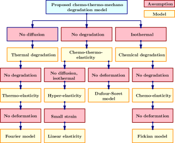
The following popular non-degradation constitutive models can be shown as special cases of the proposed degradation model, as shown in Figure 2, when the material parameters are assumed to be independent of concentration, temperature, and deformation of the solid. That is, the Lamé parameters and $\mathbf{D}_{\alpha\beta}$ ($\alpha$ and $\beta$ represent either $\vartheta$ or $\varkappa$) are independent of $c$, $\vartheta$, and $\mathbf{E}$.

1. Fourier and Fickian models: The standard heat conduction constitutive model is obtained by assuming the solid to be rigid and mass concentration of diffusing chemical species to be equal to zero. Similarly, to recover the standard Fickian model we assume the solid to be rigid and temperature of the homogenized body to be constant.

2. Dufour-Soret model: This model is obtained by assuming the solid to be rigid. Furthermore, the thermo-chemo coupling parameter $d_{\vartheta c}$ is neglected.

3. Linearized elasticity and hyperelasticity: To obtain hyperelastic constitutive models, we assume isothermal conditions and mass concentration of diffusing chemical species to be equal to zero. The linearized elasticity model can be recovered from any given hyperelastic model by assuming that the small strains assumption given by equation (2.9) holds.

4. Thermoelasticity: The standard thermoelasticity model can be recovered by assuming mass concentration of diffusing chemical species to be equal to zero. The material parameters are assumed to be independent of temperature and deformation.

5. Chemoelasticity:  Similarly, the standard chemoelasticity model can be recovered by assuming isothermal conditions. The material parameters are assumed to be independent of concentration and deformation.

6. Chemo-Thermoelasticity: Herein, we assume that the material parameters are independent of concentration, temperature, and deformation. In addition, thermo-chemo coupling parameter $d_{\vartheta c}$, Dufour tensor, and Soret tensor are neglected.

One can also derive specialized (thermo-mechano and chemo-mechano) degradation models:

1. Thermo-mechano degradation model: This model is obtained from the thermoelasticity model by relaxing the assumption that material parameters are independent of temperature and deformation.

2. Chemo-mechano degradation model: Similar to thermo-mechano degradation model, this degradation model is obtained from the chemoelasticity model by relaxing the assumption that material parameters are independent of concentration and deformation.

Figure 2. Special cases of the proposed chemo-thermo-mechano degradation model: Many existing degrading and non-degrading constitutive models are special cases of the proposed hierarchical model, with appropriate assumptions.

3.2.1. Status of the degradation model in [Mudunuru and Nakshatrala, 2012]

The small-strain chemo-mechano degradation model proposed in [Mudunuru and Nakshatrala, 2012] is a special case of the proposed chemo-thermo-mechano degradation, and can be obtained under a plethora of assumptions. These assumptions include steady-state response, small strains, and isothermal conditions with negative volumetric heat source in the entire degrading body. One also needs to neglect chemo-thermo, chemo-mechano, and thermo-mechano couplings. Moreover, the functional forms of the specific Helmholtz potential and rate of dissipation functional need to be:

$$A =\frac{1}{\rho}\psi+\frac{R_{s}\vartheta_{\mathrm{ref}}}{2}\{c-c_{\mathrm{ref}}\}^{2}$$ (3.18)

$$\zeta =\frac{1}{R_{s}\vartheta_{\mathrm{ref}}}\mathrm{grad}[\varkappa]\bullet\mathbf{D}_{\varkappa\varkappa}\mathrm{grad}[\varkappa]$$ (3.19)

where the stored strain energy density functional is given by:

$$\psi=\hat{\psi}(\mathbf{E}_{l},c)=\frac{\lambda(c)}{2}\left(\mathrm{tr}[\mathbf{E}_{l}]\right)^{2}+\mu(c)\mathbf{E}_{l}\bullet\mathbf{E}_{l}$$ (3.20)

Under the small strain assumption given by equation (2.9), the Cauchy stress, chemical potential, and mass transfer flux vector can be written as:

$$\mathbf{T}=\rho\frac{\partial A}{\partial\mathbf{E}_{l}}=\lambda(c)\mathrm{tr}[\mathbf{E}_{l}]\mathbf{I}+2\mu(c)\mathbf{E}_{l}$$ (3.21)

$$\varkappa=\frac{\partial A}{\partial c}=R_{s}\vartheta_{\mathrm{ref}}\{c-c_{\mathrm{ref}}\}$$ (3.22)

$$\mathbf{h}=-\frac{1}{2}\rho\frac{\partial\hat{\zeta}}{\partial\mathrm{grad}[\varkappa]}=-\frac{\rho}{R_{s}\vartheta_{\mathrm{ref}}}\mathbf{D}_{\varkappa\varkappa}\mathrm{grad}[\varkappa]$$ (3.23)

The balance of chemical species and the balance of linear momentum for the solid are given by equations (2.13) and (2.14). Under the isothermal condition, the balance of energy simplifies to the following expression:

$$q=-\frac{\rho}{R_{s}\vartheta_{\mathrm{ref}}}\mathrm{grad}[\varkappa]\bullet\mathbf{D}_{\varkappa\varkappa}\mathrm{grad}[\varkappa]$$ (3.24)

which means that $q$ needs to be non-positive in order to maintain the isothermal condition. The deformation dependent diffusivity $\mathbf{D}_{\varkappa\varkappa}$ is based on the small strain assumption, which is obtained by linearizing the equations (3.1.1) and (3.1.1). Note that this model is developed based on the experimental evidence that the relative diffusion rate varies exponentially with respect to the trace of strain [McAfee, 1958a, b]. In this paper, we have taken a step further to calibrate these materials parameters according to the experimental data for finite strains based on the model given by equations (3.1.1) and (3.1.1).

4. CALIBRATION WITH EXPERIMENTAL DATA

In this section, we will calibrate the proposed model for the diffusivity using the experimental data set reported in [McAfee, 1958a, b]. These experiments were conducted on spherical shells made of glass, which is a brittle material. These papers report the variation of diffusivity under various deformation modes: tension, compression, and shear. The calibration study presented below, which also includes a statistical analysis of the fit, will be valuable in two ways. First, it demonstrates the predictive capabilities of the proposed constitutive model, and provides confidence in the model to be able to apply to other brittle materials like ceramics and even to quasi-brittle materials like concrete with appropriate modifications. Second, it provides order-of-magnitude estimates for various parameters in the diffusivity model for realistic materials. This will guide in the selection of values for these parameters in the subsequent numerical studies.

Figure 3. Calibration with experimental data: A pictorial description of the degrading shell used for calibrating the proposed model with the experimental data.

Figure 3 provides the geometry and the loading on a spherical shell. The inner and outer radii are, respectively, $a=0.99$ and $b=1.0$. The boundary conditions for the deformation subproblem is that the pressure within the sphere is varied from $p_{i}=0$ to $p_{i}=0.68947\,\mathrm{MPa}$ ($100\,\mathrm{psi}$) and the external surface is traction free. For the diffusion subproblem, $c(a)=0$ and $c(b)=1$. In this scenario, it can be assumed that the tensile strain is predominant. The diffusion can be assumed to be isotropic. Hence, equation (3.1.1) is simplified as follows:

$$D=D_{0}+\left(D_{T}-D_{0}\right)\frac{\left(\exp[\eta_{T}I_{\mathbf{E}}]-1\right)}{\left(\exp[\eta_{T}E_{\mathrm{ref}_{T}}]-1\right)}$$ (4.1)

The sample size to estimate the parameters in the proposed deformation-diffusivity model has been taken to be 3. It has been reported that $D_{0}=7.26\times 10^{-13}\mathrm{m}^{2}/\mathrm{sec}^{-1}$ for glass fibers by [McAfee, 1958a]. Based on the chosen sample size and value of $D_{0}$, the estimated diffusivity parameters are given as follows:

$$\eta_{T}=1.43\times 10^{4},\ D_{T}=23.39\times 10^{-13},\ E_{\mathrm{ref}_{T}}=1.833\times 10^{-3}$$ (4.2)

Using the experimental data reported in [McAfee, 1958b] under compressive and shear strains, and following a similar procedure as before, the following diffusivity parameters are obtained:

$$\eta_{C}=401.19,\ D_{C}=8.66\times 10^{-13},\ E_{\mathrm{ref}_{C}}=1.0\times 10^{-3}$$ (4.3a)

$$\eta_{S}=-239.61,\ D_{S}=8.65\times 10^{-13},\ E_{\mathrm{ref}_{S}}=3.0\times 10^{-3}$$ (4.3b)

Figure 4. Calibration with experimental data: This figure compares the experimental data reported in [McAfee, 1958a, b] with the proposed constitutive model. The sample size is taken to be 3. The strain invariants are given by equations (3.14a)–(3.14b). A good agreement has been observed between the experimental data and the proposed constitutive model for the diffusivity under tensile, compressive, and shear strains.

We then compared the proposed model (which is obtained based on sample size of 3 points) with the experimental data set of 10 points. Figure 4 shows the relation between the relative diffusion coefficient $D/D_{0}$ and various strain invariants. From this figure, it is evident that the proposed model is in a good agreement with the experimental data. Table 3 provides a statistical analysis on the fit of the experimental data with the proposed model. The coefficient of determination is close to 1. This means that the proposed model based on parameter set given by equations (4.2)–(4.3b) is a good fit to the set of experimental data of various sample sizes. To calibrate $\mathbf{D}_{MS}$, $\eta_{MS}$, and $E_{\mathrm{ref}MS}$, we need additional experimental data related to mode of shear. However, such a data set to calibrate the effect of distortion due to shear on the diffusivity of glass is not available in literature yet. Hence, we could not calibrate $\mathbf{D}_{MS}$, $\eta_{MS}$, and $E_{\mathrm{ref}MS}$. Whenever such an experimental data is available, one can easily calibrate these parameters in a similar fashion.

Table 3. A statistical analysis of the fit: This table provides the goodness of fit of the proposed model with the experimental data set reported in [McAfee, 1958a, b]. Analysis is performed for various extracted sample sizes, and under tension, compression and shear strains. It is observed that the coefficient of determination is close to 1.

Sample size	Mean data			Standard deviation data			Coefficient of determination
	Tension	Compression	Shear	Tension	Compression	Shear	Tension	Compression	Shear
$10$	1.507	1.093	1.114	0.526	0.073	0.068	0.988	0.999	0.997
$25$	1.505	1.094	1.108	0.511	0.062	0.065	0.986	0.999	0.997
$50$	1.521	1.095	1.107	0.515	0.062	0.062	0.987	0.999	0.997
$75$	1.391	1.097	1.115	0.468	0.062	0.059	0.984	0.999	0.997

5. INITIAL BOUNDARY VALUE PROBLEM AND MATHEMATICAL ANALYSIS

From the above statements, the governing equations for the proposed chemo-thermo-mechano degrading model are stated as follows. Let the boundary of $\Omega_{0}(\mathfrak{B})$ be denoted as $\partial\Omega_{0}$ and the corresponding unit outward normal to this boundary be denoted by $\widehat{\mathbf{n}}_{0}(\mathbf{p})$. Similarly, $\partial\Omega_{t}$ denotes the boundary of $\Omega_{t}(\mathfrak{B})$ and the corresponding unit outward normal to this boundary is denoted by $\widehat{\mathbf{n}}(\mathbf{x},t)$. For the deformation subproblem, the boundary is divided into two complementary parts: $\Gamma^{\mathrm{D}}_{u}$ and $\Gamma^{\mathrm{N}}_{u}$ such that $\Gamma^{\mathrm{D}}_{u}\cup\Gamma^{\mathrm{N}}_{u}=\partial\Omega_{0}$ and $\Gamma^{\mathrm{D}}_{u}\cap\Gamma^{\mathrm{N}}_{u}=\emptyset$. $\Gamma^{\mathrm{D}}_{u}$ is the part of the boundary on which displacement is prescribed and $\Gamma^{\mathrm{N}}_{u}$ is the part of the boundary on which traction is prescribed.

Similarly, for the transport and thermal subproblem, the boundary is divided into complementary parts: $\Gamma^{\mathrm{D}}_{c}$ and $\Gamma^{\mathrm{N}}_{c}$ and $\Gamma^{\mathrm{D}}_{\vartheta}$ and $\Gamma^{\mathrm{N}}_{\vartheta}$ such that $\Gamma^{\mathrm{D}}_{c}\cup\Gamma^{\mathrm{N}}_{c}=\partial\Omega_{0}$, $\Gamma^{\mathrm{D}}_{\vartheta}\cup\Gamma^{\mathrm{N}}_{\vartheta}=\partial\Omega$, $\Gamma^{\mathrm{D}}_{c}\cap\Gamma^{\mathrm{N}}_{c}=\emptyset$, and $\Gamma^{\mathrm{D}}_{\vartheta}\cap\Gamma^{\mathrm{N}}_{\vartheta}=\emptyset$. $\Gamma^{\mathrm{D}}_{c}$ is the part of the boundary on which concentration is prescribed. $\Gamma^{\mathrm{N}}_{c}$ is the part of the boundary on which total/diffusive flux is prescribed. $\Gamma^{\mathrm{D}}_{\vartheta}$ is the part of the boundary on which temperature is prescribed. $\Gamma^{\mathrm{N}}_{\vartheta}$ is the part of the boundary on which thermal flux is prescribed. In case of steady-state analysis, it should be noted that the $\mathrm{meas}\left(\Gamma^{\mathrm{D}}_{c}\right)>0$, $\mathrm{meas}\left(\Gamma^{\mathrm{D}}_{\vartheta}\right)>0$, and $\mathrm{meas}\left(\Gamma^{\mathrm{D}}_{u}\right)>0$. However, such a condition is not required for studying transient problems.

5.1. Governing equations of the proposed model

The governing equations for the deformation sub-problem take the following form:

$$\rho_{0}\dot{\mathbf{v}}(\mathbf{p},t)=\mathrm{Div}[\mathbf{P}]+\rho_{0}\mathbf{b}(\mathbf{p},t)\quad \mathrm{in}\;\Omega_{0}\times]0,\mathcal{I}[$$ (5.1a)

$$\mathbf{u}(\mathbf{p},t)=\mathbf{u}^{\mathrm{p}}(\mathbf{p},t)\quad \mathrm{on}\;\Gamma^{\mathrm{D}}_{u}\times]0,\mathcal{I}[$$ (5.1b)

$$\mathbf{P}\widehat{\mathbf{n}}_{0}(\mathbf{p})=\mathbf{t}^{\mathrm{p}}(\mathbf{p},t)\quad \mathrm{on}\;\Gamma^{\mathrm{N}}_{u}\times]0,\mathcal{I}[$$ (5.1c)

$$\mathbf{u}(\mathbf{p},t=0)=\mathbf{u}^{\mathrm{i}}(\mathbf{p})\quad \mathrm{in}\;\Omega_{0}$$ (5.1d)

$$\mathbf{v}(\mathbf{p},t=0)=\mathbf{v}^{\mathrm{i}}(\mathbf{p})\quad \mathrm{in}\;\Omega_{0}$$ (5.1e)

where $\mathbf{u}^{\mathrm{p}}(\mathbf{p},t)$ denotes the prescribed displacement on the boundary and $\mathbf{t}^{\mathrm{p}}(\mathbf{p},t)$ is the prescribed traction on the boundary. $\mathbf{u}^{\mathrm{i}}(\mathbf{p})$ and $\mathbf{v}^{\mathrm{i}}(\mathbf{p})$ are the initial conditions for the displacement and velocity, respectively.

The governing equations for the transport sub-problem take the following form:

$$\rho_{0}\dot{c}(\mathbf{p},t)+\mathrm{Div}[\mathbf{h}_{0}]=h_{0}(\mathbf{p},t)\quad \mathrm{in}\;\Omega_{0}\times]0,\mathcal{I}[$$ (5.2a)

$$c(\mathbf{p},t)=c^{\mathrm{p}}(\mathbf{p},t)\quad \mathrm{on}\;\Gamma^{\mathrm{D}}_{c}\times]0,\mathcal{I}[$$ (5.2b)

$$\mathbf{h}_{0}\bullet\widehat{\mathbf{n}}_{0}(\mathbf{p})=h^{\mathrm{p}}(\mathbf{p},t)\quad \mathrm{on}\;\Gamma^{\mathrm{N}}_{c}\times]0,\mathcal{I}[$$ (5.2c)

$$c(\mathbf{p},t=0)=c^{\mathrm{i}}(\mathbf{p})\quad \mathrm{in}\;\Omega_{0}$$ (5.2d)

where $c^{\mathrm{p}}(\mathbf{p},t)$ denotes the prescribed concentration on the boundary, $h^{\mathrm{p}}(\mathbf{p},t)$ is the prescribed total/diffusive flux on the boundary, and $c^{\mathrm{i}}(\mathbf{p})$ is the initial condition for the concentration field.

The governing equations for the thermal sub-problem take the following form:

$$\rho_{0}\vartheta(\mathbf{p},t)\dot{\eta}=-\mathrm{Div}[\mathbf{q}_{0}]-\mathrm{Grad}[\varkappa]\bullet\mathbf{h}_{0}+q_{0}(\mathbf{p},t) \quad\mathrm{in}\;\Omega_{0}\times]0,\mathcal{I}[$$ (5.3a)

$$\vartheta(\mathbf{p},t)=\vartheta^{\mathrm{p}}(\mathbf{p},t) \quad\mathrm{on}\;\Gamma^{\mathrm{D}}_{\vartheta}\times]0,\mathcal{I}[$$ (5.3b)

$$\mathbf{q}_{0}\bullet\widehat{\mathbf{n}}_{0}(\mathbf{p})=q^{\mathrm{p}}(\mathbf{p},t) \quad\mathrm{on}\;\Gamma^{\mathrm{N}}_{c}\times]0,\mathcal{I}[$$ (5.3c)

$$\vartheta(\mathbf{p},t=0)=\vartheta^{\mathrm{i}}(\mathbf{p}) \quad\mathrm{in}\;\Omega_{0}$$ (5.3d)

where $\vartheta^{\mathrm{p}}(\mathbf{p},t)$ denotes the prescribed temperature on the boundary, $q^{\mathrm{p}}(\mathbf{p},t)$ is the prescribed heat flux on the boundary, and $\vartheta^{\mathrm{i}}(\mathbf{p})$ is the initial condition for the temperature field.

5.2. On the stability of unsteady solutions

We now show that the unsteady solutions under the proposed mathematical model for degradation are stable in the sense of a dynamical system. There are different notions of stability, and herein we shall establish the stability in the sense of Lyapunov [Dym, 2002]. For the entire analysis presented in this section, we assume homogeneous Dirichlet boundary conditions on the entire boundary for the diffusion and thermal sub-problems. Let

$$\boldsymbol{\chi}:=\left\{\begin{array}[]{c}\boldsymbol{\varphi}\\ \mathbf{v}\\ \vartheta\\ c\end{array}\right\}$$ (5.8)

Consider the following functional, which is defined on the reference configuration:

$$\mathbb{V}(\boldsymbol{\chi}):=\displaystyle\int\limits_{\Omega_{0}(\mathfrak{B})}\rho_{0}\left(A+\vartheta\eta+\frac{1}{2}\mathbf{v}\bullet\mathbf{v}\right)\;\mathrm{d}\Omega_{0}+\Pi_{\mathrm{mech},\mathrm{ext}}(\boldsymbol{\varphi})$$ (5.9)

where $\Pi_{\mathrm{mech},\mathrm{ext}}(\boldsymbol{\varphi})$ is the potential energy due to external mechanical loading, which is assumed to be conservative. This implies the following

$$\frac{\mathrm{d}}{\mathrm{d}t}\Pi_{\mathrm{mech},\mathrm{ext}}(\boldsymbol{\varphi})=-\int_{\Omega_{0}(\mathfrak{B})}\rho_{0}\mathbf{b}\bullet\mathbf{v}\;\mathrm{d}\Omega_{0}-\int_{\Gamma_{u}^{\mathrm{N}}}\mathbf{t}^{\mathrm{p}}\bullet\mathbf{v}\;\mathrm{d}\Gamma_{0}$$ (5.10)

In the literature, the above functional has been shown to be a Lyapunov functional for linearized thermoelasticity and for themo-hyperelasticity. For example, see [Ericksen, 1966; Coleman and Dill, 1973; Gurtin, 1975] and references therein. Herein, we shall show that the above functional is a legitimate Lyapunov functional for the proposed degradation model, and specifically use the Lyapunov’s second method for stability (which is a classical result in the theory of dynamical systems; for example, see [Hale and Kocak, 1991; Strogatz, 2001; Wiggins, 2003]) to establish the stability of the solutions under the proposed degradation model.

To this end, we shall take the reference or equilibrium state as:

$$\boldsymbol{\chi}_{\mathrm{eq}}:=\left\{\begin{array}[]{c}\boldsymbol{\varphi}_{\mathrm{eq}}\\ \mathbf{0}\\ 0\\ 0\end{array}\right\}$$ (5.15)

where $\boldsymbol{\varphi}_{\mathrm{eq}}$ is the static equilibrium deformation. The above functional is a candidate for Lyapunov functional, as it satisfies:

$$\mathbb{V}(\boldsymbol{\chi}=\boldsymbol{\chi}_{\mathrm{eq}})=0\quad\mathrm{and}\quad\mathbb{V}(\boldsymbol{\chi}\neq\boldsymbol{\chi}_{\mathrm{eq}})>0$$ (5.16)

We now show that

$$\frac{\mathrm{d}\mathbb{V}}{\mathrm{d}t}\leq 0$$ (5.17)

$$\frac{\mathrm{d}\mathbb{V}}{\mathrm{d}t} =\displaystyle\int\limits_{\Omega_{0}(\mathfrak{B})}\rho_{0}\left(\frac{\partial A}{\partial\mathbf{F}}\bullet\dot{\mathbf{F}}+\frac{\partial A}{\partial\vartheta}\dot{\vartheta}+\frac{\partial A}{\partial c}\dot{c}+\dot{\vartheta}\eta+\vartheta\dot{\eta}+\mathbf{v}\bullet\dot{\mathbf{v}}\right)\;\mathrm{d}\Omega_{0}+\frac{\mathrm{d}}{\mathrm{d}t}\Pi_{\mathrm{mech,ext}}(\boldsymbol{\varphi})$$

$$=\displaystyle\int\limits_{\Omega_{0}(\mathfrak{B})}\rho_{0}\left(\varkappa\dot{c}+\vartheta\dot{\eta}\right)\;\mathrm{d}\Omega_{0}+\displaystyle\int\limits_{\Omega_{0}(\mathfrak{B})}\rho_{0}\left(\frac{\partial A}{\partial\vartheta}+\eta\right)\dot{\vartheta}\;\mathrm{d}\Omega_{0}+\displaystyle\int\limits_{\Omega_{0}(\mathfrak{B})}\left(\rho_{0}\mathbf{v}\bullet\dot{\mathbf{v}}+\mathbf{P}\bullet\dot{\mathbf{F}}\right)\;\mathrm{d}\Omega_{0}+\frac{\mathrm{d}}{\mathrm{d}t}\Pi_{\mathrm{mech,ext}}(\boldsymbol{\varphi})$$

$$=\displaystyle\int\limits_{\Omega_{0}(\mathfrak{B})}\rho_{0}\left(\varkappa\dot{c}+\vartheta\dot{\eta}\right)\;\mathrm{d}\Omega_{0}$$

$$=-\displaystyle\int\limits_{\Omega_{0}(\mathfrak{B})}\varkappa\mathrm{Div}[\mathbf{h}_{0}]\;\mathrm{d}\Omega_{0}-\displaystyle\int\limits_{\Omega_{0}(\mathfrak{B})}\frac{\vartheta-\vartheta_{\mathrm{ref}}}{\vartheta}\mathrm{Div}[\mathbf{q}_{0}]\;\mathrm{d}\Omega_{0}-\displaystyle\int\limits_{\Omega_{0}(\mathfrak{B})}\frac{\vartheta-\vartheta_{\mathrm{ref}}}{\vartheta}\mathrm{Grad}[\varkappa]\bullet\mathbf{h}_{0}\;\mathrm{d}\Omega_{0}$$

$$=\displaystyle\int\limits_{\Omega_{0}(\mathfrak{B})}\mathrm{Grad}[\varkappa]\bullet\mathbf{h}_{0}\;\mathrm{d}\Omega_{0}-\displaystyle\int\limits_{\Omega_{0}(\mathfrak{B})}\left(1-\frac{\vartheta_{\mathrm{ref}}}{\vartheta}\right)\mathrm{Div}[\mathbf{q}_{0}]\;\mathrm{d}\Omega_{0}-\displaystyle\int\limits_{\Omega_{0}(\mathfrak{B})}\left(1-\frac{\vartheta_{\mathrm{ref}}}{\vartheta}\right)\mathrm{Grad}[\varkappa]\bullet\mathbf{h}_{0}\;\mathrm{d}\Omega_{0}$$

$$=\displaystyle\int\limits_{\Omega_{0}(\mathfrak{B})}\frac{\vartheta_{\mathrm{ref}}}{\vartheta}\left(\frac{1}{\vartheta}\mathrm{Grad}[\vartheta]\bullet\mathbf{q}_{0}+\mathrm{Grad}[\varkappa]\bullet\mathbf{h}_{0}\right)\;\mathrm{d}\Omega_{0}=-\displaystyle\int\limits_{\Omega_{0}(\mathfrak{B})}\frac{\vartheta_{\mathrm{ref}}}{\vartheta}\zeta_{0}\;\mathrm{d}\Omega_{0}$$ (5.18)

Since $\zeta_{0}>0$ if $\boldsymbol{\chi}\neq\boldsymbol{\chi}_{\mathrm{eq}}$, $\vartheta,\,\vartheta_{\mathrm{ref}}>0$, one can conclude that

$$\frac{\mathrm{d}\mathbb{V}}{\mathrm{d}t}<0$$ (5.19)

From the Lyapunov stability of continuous systems [Dym, 2002; Hale and Kocak, 1991], one can conclude that $\boldsymbol{\chi}=\boldsymbol{\chi}_{\mathrm{eq}}$ is asymptotically stable.

6. SEMI-ANALYTICAL SOLUTIONS TO CANONICAL PROBLEMS

In this section, we shall appeal to semi-inverse methods to obtain solutions to some popular canonical boundary value problems [Ogden, 1997]. Incompressible neo–Hookean chemo-thermo-mechano degradation model is considered here. Similar analysis can be performed for other compressible and incompressible chemo-mechano, thermo-mechano, and chemo-thermo-mechano degradation models. Coordinate system under consideration is either spherical or cylindrical. In all the problems discussed below, we assume concentration and temperature to be functions of time $t$ and radius $r$ (which is a current configuration variable). This assumption is often made because the underlying problem has either cylindrical or spherical symmetry. We also assume that the volumetric sources corresponding to temperature and concentration are equal to zero. In this paper, as we are mainly interested in degradation of solid due to temperature and transport of chemical species, we shall neglect Dufour effect, Soret effect, thermo-chemo coupling parameter $d_{\vartheta c}$, and anisotropic coefficient of thermal and chemical expansions. In order to reduce the complexity of finding solutions based on semi-inverse method for deformation sub-problem, we shall neglect the inertial effects and body forces.

Based on the assumptions provided here, the governing equations for the transport sub-problem in cylindrical coordinates reduce to:

$$\rho\frac{\partial c}{\partial t}+\frac{1}{r}\frac{\partial rh_{r}}{\partial r}=0,\;c(r=r_{i},t)=c_{i},\;c(r=r_{o},t)=c_{o},\;c(r,t=0) =c_{0}$$ (6.1)

where $h_{r}$ is the mass transfer flux in the radial direction. Similarly, the governing equations for the thermal sub-problem in cylindrical coordinates can be written as:

$$\rho\vartheta\frac{\partial\eta}{\partial t}+\frac{1}{r}\frac{\partial rq_{r}}{\partial r}=-\frac{\partial\varkappa}{\partial r}h_{\mathrm{r}},\;\vartheta(r=r_{i},t)=\vartheta_{i},\;\vartheta(r=r_{o},t)=\vartheta_{o},\;\vartheta(r,t=0)=\vartheta_{0}$$ (6.2)

where $q_{r}$ is the heat flux in the radial direction. In spherical coordinates, the governing equations for the transport sub-problem are:

$$\rho\frac{\partial c}{\partial t}+\frac{1}{r^{2}}\frac{\partial r^{2}h_{r}}{\partial r}=0,\;c(r=r_{i},t)=c_{i},\;c(r=r_{o},t)=c_{o},\;c(r,t=0)=c_{0}$$ (6.3)

The governing equations for the thermal sub-problem in spherical coordinates are:

$$\rho\vartheta\frac{\partial\eta}{\partial t}+\frac{1}{r^{2}}\frac{\partial r^{2}q_{r}}{\partial r}=-\frac{\partial\varkappa}{\partial r}h_{\mathrm{r}},\;\vartheta(r=r_{i},t)=\vartheta_{i},\;\vartheta(r=r_{o},t)=\vartheta_{o},\;\vartheta(r,t=0)=\vartheta_{0}$$ (6.4)

Another quantity of interest in material degradation is the extent of damage at a particular location or along the cross-section of the degrading body. In case of incompressible neo-Hookean chemo-thermo-mechano degradation model, this quantity can be defined as follows:

$$\mathcal{D}_{\mu}(\mathbf{x},t):=\frac{\mu}{\mu_{0}}=1-\left(\frac{\mu_{1}c}{\mu_{0}c_{\mathrm{ref}}}\right)-\left(\frac{\mu_{2}\vartheta}{\mu_{0}\vartheta_{\mathrm{ref}}}\right)$$ (6.5)

For virgin material, $\mathcal{D}_{\mu}=1$. If $\mathcal{D}_{\mu}$ approaches zero, then the material has degraded the most. In addition, equation (6.5) also provides the following information:

• Amount of degradation at a given location and time,

• The parts of the body that suffered extensive damage, and

• The effect of temperature and moisture (or concentration of chemical species) on the mechanical properties of materials.

6.1. Inflation of a degrading spherical shell

We now study the behavior of a degrading (thick) spherical shell subjected to pressure loading. Figure 5 provides a pictorial description of the boundary value problem. In addition to the obvious theoretical significance, this problem has relevance to safety, reliability and defect monitoring of degrading spherical structures (such as a tank shell and a bearing structure) due to pressure loading.

Due to the spherical symmetric associated with the problem, spherical coordinates are used to analyze the inflation of degrading spherical shell. Consider a spherical body of inner radius $R_{i}$ and outer radius $R_{o}$ defined in the reference configuration as follows:

$$R_{i}\leq R\leq R_{o},\quad 0\leq\Theta\leq\pi,\quad 0\leq\Phi\leq 2\pi$$ (6.6)

where $(R,\Theta,\Phi)$ are the spherical polar coordinates in the reference configuration. The inner and outer surfaces $R=R_{i}$ and $R=R_{o}$ are, respectively, subjected to pressures $p_{i}$ and $p_{o}$ with $p_{i}\geq p_{o}$. That is, the thick cylinder is inflated with pressure. The deformation in the current configuration can be described as follows:

$$r_{i}\leq r=m(R)\leq r_{o},\quad\theta=\Theta,\quad\phi=\Phi$$ (6.7)

where $(r,\theta,\phi)$ are the spherical polar coordinates in the current configuration, and $r_{i}$ and $r_{o}$ are, respectively, the inner and outer radii of the shell in the current (deformed) configuration. The deformation gradient, the left Cauchy-Green tensor, and the right Cauchy-Green tensor have the following matrix representations:

$$\left\{\mathbf{F}\right\}=\left(\begin{array}[]{ccc}\frac{dm}{dR}&0&0\\ 0&\frac{m}{R}&0\\ 0&0&\frac{m}{R}\\ \end{array}\right),\quad\left\{\mathbf{C}\right\}=\left\{\mathbf{B}\right\}=\left(\begin{array}[]{ccc}\left(\frac{dm}{dR}\right)^{2}&0&0\\ 0&\frac{m^{2}}{R^{2}}&0\\ 0&0&\frac{m^{2}}{R^{2}}\\ \end{array}\right)$$ (6.14)

Incompressibility implies that

$$r=m(R)=\sqrt[3]{R^{3}+r^{3}_{i}-R^{3}_{i}}\qquad r_{i}\leq r\leq r_{o}$$ (6.15)

where $r_{o}=\sqrt[3]{R_{o}^{3}+r^{3}_{i}-R^{3}_{i}}$. The non-zero components of the Cauchy stress are:

$$T_{rr}=-p+\mu(c,\vartheta)\left(\frac{\mathrm{d}m}{\mathrm{d}R}\right)^{2}=-p+\mu(c,\vartheta)\frac{R^{4}}{r^{4}},\quad T_{\theta\theta}=T_{\phi\phi}=-p+\mu(c,\vartheta)\frac{r^{2}}{R^{2}}$$ (6.16)

The governing equations for the balance of linear momentum in the spherical polar coordinates (e.g., see [Sadd, 2014]) reduce to:

$$\frac{\partial T_{rr}}{\partial r}+\frac{2T_{rr}-T_{\theta\theta}-T_{\phi\phi}}{r}=0,\;\frac{\partial p}{\partial\theta}=0,\;\frac{\partial p}{\partial\phi}=0$$ (6.17)

The above equations imply that $p$ is independent of $\theta$ and $\phi$. That is,

$$p=p(r,t)$$ (6.18)

From equation (3.6) and (3.7), the specific chemical potential and specific entropy for the degrading spherical shell are given as follows:

$$\varkappa =\frac{1}{\rho_{0}}\frac{\partial\psi}{\partial c}+R_{s}\vartheta_{\mathrm{ref}}\{c-c_{\mathrm{ref}}\}=-\frac{\mu_{1}}{2\rho_{0}c_{\mathrm{ref}}}\left(\frac{R^{4}}{r^{4}}+2\frac{r^{2}}{R^{2}}-3\right)+R_{s}\vartheta_{\mathrm{ref}}\{c-c_{\mathrm{ref}}\}$$ (6.19a)

$$\eta =-\frac{1}{\rho_{0}}\frac{\partial\psi}{\partial\vartheta}+\frac{c_{p}}{\vartheta_{\mathrm{ref}}}\{\vartheta-\vartheta_{\mathrm{ref}}\}=\frac{\mu_{1}}{2\rho_{0}\vartheta_{\mathrm{ref}}}\left(\frac{R^{4}}{r^{4}}+2\frac{r^{2}}{R^{2}}-3\right)+\frac{c_{p}}{\vartheta_{\mathrm{ref}}}\{\vartheta-\vartheta_{\mathrm{ref}}\}$$ (6.19b)

Before deriving the governing equations for the degrading shell problem, we shall do the non-dimensionalization by choosing primary variables and associated reference quantities that are convenient for studying this problem. To distinguish, we shall denote all the non-dimensional quantities using a superposed bar. We shall take $\mu_{0}$, $R_{o}$, $\vartheta_{\mathrm{ref}}$, $c_{\mathrm{ref}}$, and $D_{0}$ as the reference quantities, which give rise to the following non-dimensional quantities:

$$\overline{r}=\frac{r}{R_{o}},\ \overline{R}=\frac{R}{R_{o}},\ \overline{D}_{\varkappa\varkappa}=\frac{D_{\varkappa\varkappa}}{D_{0}},\ \overline{D}_{\vartheta\vartheta}=\frac{D_{\vartheta\vartheta}}{D_{0}}$$ (6.20)

$$\overline{\mu}_{1}=\frac{\mu_{1}}{\mu_{0}},\ \overline{\mu}_{2}=\frac{\mu_{2}}{\mu_{0}},\ \overline{c}=\frac{c}{c_{\mathrm{ref}}},\ \overline{\vartheta}=\frac{\vartheta}{\vartheta_{\mathrm{ref}}},\ \overline{t}=\frac{D_{0}t}{R_{o}^{2}}$$ (6.21)

With the stress field in equation (6.16), we shall integrate equation (6.17) and then have the following non-linear equation in deformation sub-problem after non-dimensionalization:

$$\overline{T}_{rr}(\overline{R}=\overline{R}_{i},\overline{t})-\overline{T}_{rr}(\overline{R}=\overline{R}_{o},\overline{t})=\overline{p}_{o}-\overline{p}_{i}=\displaystyle\int\limits_{\overline{R}_{i}}^{\overline{R}_{o}}\frac{2\overline{\mu}(\overline{c},\overline{\vartheta})\left(\overline{R}^{6}-\left(\overline{R}^{3}+\overline{r}_{i}^{3}-\overline{R}_{i}^{3}\right)^{2}\right)}{\left(\overline{R}^{3}+\overline{r}_{i}^{3}-\overline{R}_{i}^{3}\right)^{\frac{7}{3}}}\mathrm{d}\overline{R}$$ (6.22)

In order to reduce the complexity in finding semi-analytical solutions, we shall assume $\frac{\partial r}{\partial t}\ll\frac{\partial\vartheta}{\partial t}$. Substituting equation (6.19a) and (6.19b) into the constitutive relations of the proposed model, the governing equations of these two sub-problems (6.3), (6.4) can be written as follows after non-dimensionalization:

$$\frac{\partial\overline{c}}{\partial\overline{t}}-\left(\frac{2\overline{D}_{\varkappa\varkappa}}{\overline{r}}+\frac{\partial\overline{D}_{\varkappa\varkappa}}{\partial\overline{r}}\right)\frac{\partial\overline{c}}{\partial\overline{r}}-\overline{D}_{\varkappa\varkappa}\frac{\partial^{2}\overline{c}}{\partial\overline{r}^{2}}=2\overline{\omega}\frac{\partial\overline{D}_{\varkappa\varkappa}}{\partial\overline{r}}\left(\frac{\overline{R}^{4}}{\overline{r}^{5}}-\frac{\overline{r}}{\overline{R}^{2}}\right)-6\overline{\omega}\overline{D}_{\varkappa\varkappa}\left(\frac{1}{\overline{R}^{2}}+\frac{\overline{R}^{4}}{\overline{r}^{6}}\right)$$ (6.23)

$$\overline{\vartheta}\frac{\partial\overline{\vartheta}}{\partial\overline{t}}-\left(2\frac{\overline{D}_{\vartheta\vartheta}}{\overline{r}}+\frac{\partial\overline{D}_{\vartheta\vartheta}}{\partial\overline{r}}\right)\frac{\partial\overline{\vartheta}}{\partial\overline{r}}-\overline{D}_{\vartheta\vartheta}\frac{\partial^{2}\overline{\vartheta}}{\partial\overline{r}^{2}}=\overline{\tau}\overline{D}_{\varkappa\varkappa}\left(\frac{\partial\overline{c}}{\partial\overline{r}}-2\overline{\omega}\left(\frac{\overline{r}}{\overline{R}^{2}}-\frac{\overline{R}^{4}}{\overline{r}^{5}}\right)\right)^{2}$$ (6.24)

where $\overline{\omega}$ and $\overline{\tau}$ are two non-dimensional parameters, which have the following expressions:

$$\overline{\omega}=\frac{\mu_{1}}{\rho_{0}R_{s}\vartheta_{\mathrm{ref}}c^{2}_{\mathrm{ref}}},\quad\overline{\tau}=\frac{R_{s}c^{2}_{\mathrm{ref}}}{c_{p}}$$ (6.25)

The non-linear equation (6.22) enables us to find $\overline{r}_{i}$ at various $\overline{t}$ for given $\overline{c}(\overline{R},\overline{t})$ and $\overline{\vartheta}(\overline{R},\overline{t})$. However, it should be noted that $\overline{c}(\overline{R},\overline{t})$ and $\overline{\vartheta}(\overline{R},\overline{t})$ are also a function of $\overline{r}_{i}$ in case of strong coupling. This is because diffusivity and thermal conductivity depend on the invariants of strain $\overline{\mathbf{E}}$. Hence, the integral equation (6.22) and partial differential equations (6.23) and (6.24) are strongly coupled.

6.1.1. Steady-state analysis for shell degradation

For steady-state, we have $h_{r}r^{2}=C_{1}$ and $q_{r}r^{2}+\varkappa h_{r}r^{2}=C_{2}$, where $C_{1}$ and $C_{2}$ are integration constants. This implies that $\overline{c}$ and $\overline{\vartheta}$ are the solutions of the following ODEs:

$$\overline{D}_{\varkappa\varkappa}\overline{r}^{2}\frac{d\overline{c}}{d\overline{r}}-2\overline{D}_{\varkappa\varkappa}\overline{\omega}\left(\frac{\overline{r}^{3}}{\overline{R}^{2}}-\frac{\overline{R}^{4}}{\overline{r}^{3}}\right)+\overline{C}_{1}=0$$ (6.26a)

$$\overline{D}_{\vartheta\vartheta}\overline{r}^{2}\frac{d\overline{\vartheta}}{d\overline{r}}+\overline{\tau}\left(\frac{\overline{w}}{2}\left(\frac{\overline{R}^{4}}{\overline{r}^{4}}+2\frac{\overline{r}^{2}}{\overline{R}^{2}}-3\right)-\overline{c}+1\right)\overline{C}_{1}+\overline{C}_{2}=0$$ (6.26b)

where the integration constants $\overline{C}_{1}$ and $\overline{C}_{2}$ are determined from the boundary conditions for the transport and thermal sub-problems. Under weak coupling (i.e., $D_{\vartheta\vartheta}$ and $D_{\varkappa\varkappa}$ are constants), a simplified form of the analytical solutions for $\overline{c}$ and $\overline{\vartheta}$ can be obtained as follows:

$$\overline{c}=\overline{\omega}\left(\frac{\overline{r}^{2}}{\overline{R}^{2}}+\frac{\overline{R}^{4}}{2\overline{r}^{4}}\right)+\frac{B_{1}}{\overline{r}}+A_{1},\quad\overline{\vartheta}=-\frac{\overline{\tau}B_{1}^{2}\overline{D}_{\varkappa\varkappa}}{2\overline{D}_{\vartheta\vartheta}\overline{r}^{2}}+\frac{Z_{1}}{\overline{r}}+Y_{1}$$ (6.27)

where $A_{1}$, $B_{1}$, $Y_{1}$, and $Z_{1}$ are constants, which are given in terms of the boundary conditions $\overline{c}_{i}$, $\overline{c}_{o}$, $\overline{\vartheta}_{i}$, and $\overline{\vartheta}_{o}$ as follows:

$$A_{1}=\overline{c}_{i}-\frac{B_{1}}{\overline{r}_{i}}-\overline{\omega}\left(\frac{\overline{r}_{i}^{2}}{\overline{R}^{2}}+\frac{8\overline{R}^{4}}{\overline{r}_{i}^{4}}\right)$$ (6.28a)

$$B_{1}=\frac{\overline{r}_{i}\overline{r}_{o}}{\overline{r}_{i}-\overline{r}_{o}}\left(\overline{c}_{o}-\overline{c}_{i}-\overline{\omega}\left(\frac{\overline{r}_{o}^{2}}{\overline{R}^{2}}+\frac{8\overline{R}^{4}}{\overline{r}_{o}^{4}}-\frac{\overline{r}_{i}^{2}}{\overline{R}^{2}}-\frac{8\overline{R}^{4}}{\overline{r}_{i}^{4}}\right)\right)$$ (6.28b)

$$Y_{1}=\overline{\vartheta}_{i}+\frac{\overline{\tau}B_{1}^{2}\overline{D}_{\varkappa\varkappa}}{2\overline{D}_{\vartheta\vartheta}\overline{r}_{i}^{2}}-\frac{Z_{1}}{\overline{r}_{i}}$$ (6.28c)

$$Z_{1}=\frac{\overline{r}_{i}-\overline{r}_{o}}{\overline{r}_{i}\overline{r}_{o}}\left(\overline{\vartheta}_{o}-\overline{\vartheta}_{i}-\frac{\overline{\tau}B_{1}^{2}\overline{D}_{\varkappa\varkappa}}{2\overline{D}_{\vartheta\vartheta}}\left(\frac{1}{\overline{r}_{i}^{2}}-\frac{1}{\overline{r}_{o}^{2}}\right)\right)$$ (6.28d)

6.1.2. Unsteady analysis for shell degradation

Herein, we shall use the method of horizontal lines [Rothe, 1930; Picard and Leis, 1980] and shooting method [Heath, 2005] to obtain numerical solutions to equations (6.23) and (6.24). In the method of horizontal lines, the time is discretized first followed by spatial discretization. The time interval of interest $[0,\overline{\mathcal{I}}]$ is divided into $N$ non-overlapping subintervals such that $\Delta\overline{t}=\frac{\overline{\mathcal{I}}}{N}$ and $\overline{t}_{n}=n\Delta\overline{t}$. $\overline{t}_{n}$ is called the integral time level, where $n=0,\cdots,N$. $\Delta\overline{t}$ is the time-step, which is assumed to be uniform. Employing the method of horizontal lines with backward Euler time-stepping scheme, we obtain the following ODEs at each time-level for equations (6.23) and (6.24):

$$\frac{d^{2}\overline{c}^{(n+1)}}{d\overline{r}^{2}} +\left(\frac{2}{\overline{r}^{(n)}}+\left(\frac{1}{\overline{D}^{(n)}_{\varkappa\varkappa}}\right)\frac{d\overline{D}_{\varkappa\varkappa}}{d\overline{r}}\Bigg{|}_{\overline{t}=\overline{t}_{n}}\right)\frac{d\overline{c}^{(n+1)}}{d\overline{r}}-\frac{\overline{c}^{(n+1)}}{\overline{D}^{(n)}_{\varkappa\varkappa}\Delta\overline{t}}=6\overline{\omega}\left(\frac{1}{\left(\overline{R}^{(n)}\right)^{2}}+\frac{\left(\overline{R}^{(n)}\right)^{4}}{\left(\overline{r}^{(n)}\right)^{6}}\right)$$

$$-\frac{\overline{c}^{(n)}}{\overline{D}^{(n)}_{\varkappa\varkappa}\Delta\overline{t}}-\left(\frac{2\overline{\omega}}{\overline{D}^{(n)}_{\varkappa\varkappa}}\right)\left(\frac{d\overline{D}_{\varkappa\varkappa}}{d\overline{r}}\Bigg{|}_{\overline{t}=\overline{t}_{n}}\right)\left(\frac{\left(\overline{R}^{(n)}\right)^{4}}{\left(\overline{r}^{(n)}\right)^{5}}-\frac{\overline{r}^{(n)}}{\left(\overline{R}^{(n)}\right)^{2}}\right)$$ (6.29)

$$\frac{d^{2}\overline{\vartheta}^{(n+1)}}{d\overline{r}^{2}} +\left(\frac{2}{\overline{r}^{(n)}}+\left(\frac{1}{\overline{D}^{(n)}_{\vartheta\vartheta}}\right)\frac{d\overline{D}_{\vartheta\vartheta}}{d\overline{r}}\Bigg{|}_{\overline{t}=\overline{t}_{n}}\right)\frac{d\overline{\vartheta}^{(n+1)}}{d\overline{r}}-\frac{\overline{\vartheta}^{(n)}\overline{\vartheta}^{(n+1)}}{\overline{D}^{(n)}_{\vartheta\vartheta}\Delta\overline{t}}=-\frac{\left(\overline{\vartheta}^{(n)}\right)^{2}}{\overline{D}^{(n)}_{\vartheta\vartheta}\Delta\overline{t}}$$

$$-\frac{\overline{\tau}\overline{D}^{(n)}_{\varkappa\varkappa}}{\overline{D}^{(n)}_{\vartheta\vartheta}}\left(\frac{d\overline{c}}{d\overline{r}}\Bigg{|}_{\overline{t}=\overline{t}_{n}}-2\overline{\omega}\left(\frac{\left(\overline{r}^{(n)}\right)}{\left(\overline{R}^{(n)}\right)^{2}}-\frac{\left(\overline{R}^{(n)}\right)^{4}}{\left(\overline{r}^{(n)}\right)^{5}}\right)\right)^{2}$$ (6.30)

where $\overline{c}^{(n)}=\overline{c}(\overline{r},\overline{t}=\overline{t}_{n})$ and $\overline{\vartheta}^{(n)}=\overline{\vartheta}(\overline{r},\overline{t}=\overline{t}_{n})$. Algorithm 1 describes a procedure to determine $\overline{c}(\overline{r},\overline{t})$, $\overline{\vartheta}(\overline{r},\overline{t})$, and $r_{i}$ at various times using an iterative non-linear numerical solution strategy. The following values are assumed for the non-dimensional parameters in the strong coupling simulations:

$$\overline{R}_{o}=1,\ \overline{R}_{i}=0.5,\ \Delta\overline{t}=0.01,\ \overline{t}=2,\ \overline{\omega}=0.05,\ \overline{\tau}=0.2,\ \overline{c}_{i}=0,\overline{\vartheta}_{0}=0.5$$

$$\overline{c}_{o}=1,\ \overline{\vartheta}_{i}=0.5,\ \overline{\vartheta}_{o}=1,\ \overline{\mu}_{0}=1,\ \overline{\mu}_{1}=0.3,\ \overline{\mu}_{2}=0.4,\ \overline{D}_{0}=1,\ \overline{D}_{T}=1.5,$$

$$\overline{D}_{S}=1.2,\ \eta_{T}=\eta_{S}=1,\ E_{\mathrm{ref}T}=E_{\mathrm{ref}S}=1,\ \overline{K}_{0}=1,\ \delta=10$$ (6.31)

In weakly coupling problem, we use $\overline{D}_{0}$, $\overline{K}_{0}$ as $\overline{D}^{(n)}_{\varkappa\varkappa}$ and $\overline{D}^{(n)}_{\vartheta\vartheta}$, respectively. It should be noted that these values are constructed based on the (brittle-type) material parameters such as glass, ceramics, and concrete.

The numerical results are shown in figures 7–11, which reveal the following conclusions on the overall behavior of degrading spherical shells under inflation:

1. Degradation vs. non-degradation: After degradation, a spherical shell which is initially homogeneous is not homogeneous anymore.

2. Due to degradation, creep-like behavior is observed. Therefore, as time progresses, hoop stresses increase. We need to note that the shell ceases to creep after a certain period of time, which is the moment when the transport of chemical species and heat conduction are close to steady-states.

3. As the pressure loading increases, the hoop stress is increasing in a non-linear fashion, which is significantly different from the non-degradation shell.

4. For non-degrading shell, the chemical potential is unchanged with respect to pressure loading. However, for strong coupling, it increases with $\overline{p}_{i}$ in a non-linear fashion when $\overline{\omega}$ is small enough. This is because for small $\overline{\omega}$, diffusion takes the dominance in the coupling effect. When pressure loading increases, the diffusivity is increasing due to the growing strain. For large $\overline{\omega}$, the deformation is dominant in the coupling, which is $-\overline{I}_{E}$ term in chemical potential. Since the first invariant $\overline{I}_{E}$ is always positive in this problem, chemical potential is decreasing when the pressure loading increases.

5. Thermo-dominated vs. chemo-dominated degradation: Weak coupling over-predicts the amount of degradation compared to the full (or strong) coupling when thermal degradation dominates. This is because when the thermal degradation dominants, the thermal conductivity decreases due to the increase in strain (note that the first invariant of strain is always positive in this problem). However, in chemo-dominated degradation, weak coupling under-predicts the amount of degradation compared to the strong coupling case.

6. In case of strong coupling, healing-like behavior is observed at early time steps in thermo-dominated degradation (but still remains below that of the virgin material). This is because variable heat sinks exist in the entire body (due to which temperature gets lower than the initial condition). Hence, the material damage is less than that of at $\overline{t}=0$. However, this heal-like behavior becomes less distinct (or even doesn’t exist) when the chemo-degradation achieves the dominance.

7. Strong vs. weak coupling: Quantitatively and qualitatively, extent of damage for both strong and weak coupling are considerably different.

Algorithm 1 Inflation of a degrading spherical shell (numerical methodology to find $\overline{r}_{i}$, $\overline{c}$, and $\overline{\vartheta}$)

1:  INPUT: Non-dimensional material parameters, non-dimensional boundary conditions, and non-dimensional initial conditions, MaxIters, tolerances $\epsilon_{\mathrm{tol}}^{(r)}$, $\epsilon_{\mathrm{tol}}^{(c)}$, and $\epsilon_{\mathrm{tol}}^{(\vartheta)}$.

2:  Evaluate $\overline{r}_{i}$ at $\overline{t}=0$ based on equation (6.22).

3:  for $n=1,2,\cdots,N$ do

4:     for $j=1,2,\cdots$ do

5:        if $j>$ MaxIters then

6:           Solution did not converge in specified maximum number of iterations. EXIT.

7:        end if

8:        Diffusion sub-problem: Given $\overline{r}^{(j)}_{i}$, solve equation (6.1.2) to obtain $\overline{c}^{(j+1)}$. Herein, we use shooting method to solve the ODEs.

9:        Heat conduction sub-problem: Given $\overline{r}^{(j)}_{i}$ and $\overline{c}^{(j+1)}$, solve equation (6.1.2) to obtain $\overline{\vartheta}^{(j+1)}$. Similarly, we use shooting method to solve the non-linear ODEs.

10:        Deformation sub-problem: Given $\overline{c}^{(j+1)}$ and $\overline{\vartheta}^{(j+1)}$, solve for $\overline{r}^{(j+1)}_{i}$ given by equation (6.22) using bisection method.

11:        if $\|\overline{r}^{(j+1)}_{i}-\overline{r}^{(j)}_{i}\|<\epsilon_{\mathrm{tol}}^{(r)}$, $\|\overline{c}^{(j+1)}-\overline{c}^{(j)}\|<\epsilon_{\mathrm{tol}}^{(c)}$, and $\|\overline{\vartheta}^{(j+1)}-\overline{\vartheta}^{(j)}\|<\epsilon_{\mathrm{tol}}^{(\vartheta)}$ then

12:           OUTPUT: $\overline{r}^{(j+1)}_{i}$, $\overline{c}^{(j+1)}$, and $\overline{\vartheta}^{(j+1)}$. EXIT.

13:        else

14:           Update the guess: $\overline{r}^{(j)}_{i}\leftarrow\overline{r}^{(j+1)}_{i}$.

15:        end if

16:     end for

17:  end for

6.2. Bending of a degrading beam

Herein, we shall consider pure bending of a degrading beam. At time $t=0$, a finite degrading beam is suddenly bent by an action of pure end moments. For $t>0$, the centerline of the beam becomes a sector of a circle of radius $r_{c}$. This centerline is held fixed for all the time. Subsequently, the stresses in the degrading beam are allowed to relax. In addition, it is assumed that the material remains isotropic with respect to the reference configuration throughout the degradation process. These assumptions enable us to employ the counterpart of universal deformations (also known as semi-inverse method) [Ogden, 1997] to study such degrading beams.

A pictorial description of the initial boundary value problem is shown in Figure 12. The degrading beam is defined as follows:

$$-L\leq X\leq L,\quad-W\leq Y\leq W,\quad-H\leq Z\leq H$$ (6.32)

where $(X,Y,Z)$ are the Cartesian coordinates in the reference configuration. We assume that the deformation to be as follows:

$$r=\sqrt{\frac{2X}{\alpha}+\beta},\quad\theta=\frac{Y}{\gamma},\quad z=Z$$ (6.33)

where $(r,\theta,z)$ are the cylindrical polar coordinates in the current configuration. When $X=0$, we have $\beta=r^{2}_{c}$. It should be noted that $\alpha$ and $\gamma$ are all unknown time-dependent parameters. These unknowns are evaluated from the incompressibility constraint, traction boundary conditions, and pure end moments. To reduce the complexity in finding semi-analytical solutions, we shall assume $r_{c}$ is given. The faces $X=-L$ and $X=L$ are subjected to ambient atmospheric pressure ‘$p_{\mathrm{atm}}$’. Upon deformation, the corresponding deformed faces $r_{i}$ and $r_{o}$ are maintained at $p_{\mathrm{atm}}$, where $r_{i}=\sqrt{r^{2}_{c}-2\gamma L}$ and $r_{o}=\sqrt{r^{2}_{c}+2\gamma L}$ are the inner and outer radius of the degrading beam. This gives the following traction boundary conditions:

$$T_{rr}(X=-L,t)=T_{rr}(X=L,t)=p_{\mathrm{atm}}$$ (6.34)

The deformation gradient $\mathbf{F}$, right Cauchy-Green tensor $\mathbf{C}$, and left Cauchy-Green tensor $\mathbf{B}$ for the degrading beam are given as follows:

$$\{\mathbf{F}\}=\left(\begin{array}[]{ccc}\frac{1}{\alpha r}&0&0\\ 0&\frac{r}{\gamma}&0\\ 0&0&1\\ \end{array}\right)\qquad\{\mathbf{C}\}=\{\mathbf{B}\}=\left(\begin{array}[]{ccc}\frac{1}{\alpha^{2}r^{2}}&0&0\\ 0&\frac{r^{2}}{\gamma^{2}}&0\\ 0&0&1\\ \end{array}\right)$$ (6.41)

For incompressible degrading neo-Hookean material, we have $\alpha\gamma=1$ and the non-zero components of the Cauchy stress tensor are given as follows:

$$T_{rr}=-p+\frac{\mu(c,\vartheta)\gamma^{2}}{2\gamma X+r^{2}_{c}},\quad T_{\theta\theta}=-p+\frac{\mu(c,\vartheta)\left(2\gamma X+r^{2}_{c}\right)}{\gamma^{2}},\quad T_{zz}=-p+\mu(c,\vartheta)$$ (6.42)

The balance of linear momentum in the cylindrical polar coordinates reduces to the following:

$$\frac{\partial T_{rr}}{\partial r}+\frac{T_{rr}-T_{\theta\theta}}{r}=0,\quad\frac{\partial p}{\partial\theta}=0,\quad\frac{\partial p}{\partial z}=0$$ (6.43)

The bending moment in the deformation sub-problem can be evaluated based on the following formula:

$$M_{\mathrm{beam}}(t) =\displaystyle\int\limits_{A_{\mathrm{cross}}}T_{\theta\theta}(r-r_{\mathrm{neu}})\mathrm{d}A$$

$$=2H\displaystyle\int\limits_{-L}^{L}T_{\theta\theta}(-\sqrt{r^{2}_{c}+2\gamma X_{\mathrm{neu}}}+\sqrt{r^{2}_{c}+2\gamma X})\frac{\gamma}{\sqrt{r^{2}_{c}+2\gamma X}}\mathrm{d}X$$ (6.44)

where $\mathrm{d}A=2H\mathrm{d}r$, $r_{\mathrm{neu}}=\sqrt{r^{2}_{c}+2\gamma X_{\mathrm{neu}}}$ is the neutral axis location, and $X_{\mathrm{neu}}$ is the value at which $T_{\theta\theta}=0$. The chemical potential, specific entropy for the degrading beam are given as follows:

$$\varkappa =\frac{1}{\rho_{0}}\frac{\partial\psi}{\partial c}+R_{s}\vartheta_{\mathrm{ref}}\{c-c_{\mathrm{ref}}\}=-\frac{\mu_{1}}{2\rho_{0}c_{\mathrm{ref}}}\left(\frac{\gamma^{2}}{r^{2}}+\frac{r^{2}}{\gamma^{2}}-2\right)+R_{s}\vartheta_{\mathrm{ref}}\{c-c_{\mathrm{ref}}\}$$ (6.45a)

$$\eta =-\frac{1}{\rho_{0}}\frac{\partial\psi}{\partial\vartheta}+\frac{c_{p}}{\vartheta_{\mathrm{ref}}}\{\vartheta-\vartheta_{\mathrm{ref}}\}=\frac{\mu_{1}}{2\rho_{0}\vartheta_{\mathrm{ref}}}\left(\frac{\gamma^{2}}{r^{2}}+\frac{r^{2}}{\gamma^{2}}-2\right)+\frac{c_{p}}{\vartheta_{\mathrm{ref}}}\{\vartheta-\vartheta_{\mathrm{ref}}\}$$ (6.45b)

Most of the non-dimensional quantities are same as that of the degrading shell problem except for the following:

$$\overline{r}=\frac{r}{r_{c}},\ \overline{X}=\frac{X}{r_{c}},\ \overline{\gamma}=\frac{\gamma}{r_{c}},\ \overline{t}=\frac{D_{0}t}{r_{c}^{2}}$$ (6.46)

Using equations (6.33)–(6.43), we have the following non-linear equation in $\overline{\gamma}$

$$\displaystyle\int\limits_{-L/r_{c}}^{L/r_{c}}\frac{\overline{\mu}(\overline{c}(\overline{X},\overline{t}),\overline{\vartheta}(\overline{X},\overline{t}))\left(\overline{\gamma}^{4}-\left(2\overline{\gamma}\overline{X}+1\right)^{2}\right)}{\overline{\gamma}\left(2\overline{\gamma}\overline{X}+1\right)^{2}}d\overline{X}=0$$ (6.47)

From (6.47), $\overline{\gamma}|_{\overline{t}=0}$ is given as follows:

$$\overline{\gamma}|_{\overline{t}=0}=\frac{1}{r_{c}}\sqrt{-2L^{2}+\sqrt{4L^{4}+r^{4}_{c}}}$$ (6.48)

which is the case for homogeneous neo-Hookean material. As $r_{c}$ is given, the parameter $\overline{\gamma}$ is bounded above and below as follows:

$$\frac{-r_{c}}{2L}<\overline{\gamma}<\frac{r_{c}}{2L}$$ (6.49)

which can be used in finding the solution for the non-linear equation given by (6.47). It should be noted that $\overline{\gamma}|_{t=0}$ satisfies the inequality given by (6.49).

From equations (6.1) and (6.2), the final form for the governing equations for transport and thermal sub-problems for degrading beam are given as follows:

$$\frac{\partial\overline{c}}{\partial\overline{t}}-\left(\frac{\overline{D}_{\varkappa\varkappa}}{\overline{r}}+\frac{\partial\overline{D}_{\varkappa\varkappa}}{\partial\overline{r}}\right)\frac{\partial\overline{c}}{\partial\overline{r}}-\overline{D}_{\varkappa\varkappa}\frac{\partial^{2}\overline{c}}{\partial\overline{r}^{2}}=\overline{\omega}\frac{\partial\overline{D}_{\varkappa\varkappa}}{\partial\overline{r}}\left(\frac{\overline{\gamma}^{2}}{\overline{r}^{3}}-\frac{\overline{r}}{\overline{\gamma}^{2}}\right)-2\overline{\omega}\overline{D}_{\varkappa\varkappa}\left(\frac{1}{\overline{\gamma}^{2}}+\frac{\overline{\gamma}^{2}}{\overline{r}^{4}}\right)$$ (6.50)

$$\overline{\vartheta}\frac{\partial\overline{\vartheta}}{\partial\overline{t}}-\left(\frac{\overline{D}_{\vartheta\vartheta}}{\overline{r}}+\frac{\partial\overline{D}_{\vartheta\vartheta}}{\partial\overline{r}}\right)\frac{\partial\overline{\vartheta}}{\partial\overline{r}}-\overline{D}_{\vartheta\vartheta}\frac{\partial^{2}\overline{\vartheta}}{\partial\overline{r}^{2}}=\overline{\tau}\overline{D}_{\varkappa\varkappa}\left(\frac{\partial\overline{c}}{\partial\overline{r}}+\overline{\omega}\left(\frac{\overline{\gamma}^{2}}{\overline{r}^{3}}-\frac{\overline{r}}{\overline{\gamma}^{2}}\right)\right)^{2}$$ (6.51)

6.2.1. Steady-state and unsteady analysis for beam degradation

In case of steady-state, we have $h_{r}r=C_{1}$ and $q_{r}r+\varkappa h_{r}r=C_{2}$, where $C_{1}$ and $C_{2}$ are integration constants. Equations (6.50) and (6.51) imply that $\overline{c}$ and $\overline{\vartheta}$ are the solutions of the following ODEs:

$$\overline{D}_{\varkappa\varkappa}\overline{r}\frac{d\overline{c}}{d\overline{r}}-\overline{D}_{\varkappa\varkappa}\overline{\omega}\left(\frac{\overline{\gamma}^{2}}{\overline{r}^{2}}-\frac{\overline{r}^{2}}{\overline{\gamma}^{2}}\right)+\overline{C}_{1}=0$$ (6.52a)

$$\overline{D}_{\vartheta\vartheta}\overline{r}\frac{d\overline{\vartheta}}{d\overline{r}}+\overline{\tau}\left(\frac{\overline{w}}{2}\left(\frac{\overline{\gamma}^{2}}{\overline{r}^{2}}+\frac{\overline{r}^{2}}{\overline{\gamma}^{2}}-2\right)-\overline{c}+1\right)\overline{C}_{1}+\overline{C}_{2}=0$$ (6.52b)

In case of weak coupling (where $D_{\vartheta\vartheta}$ and $D_{\varkappa\varkappa}$ are constants), the solutions for $\overline{c}$ and $\overline{\vartheta}$ take the following simplified form:

$$\overline{c}=-\frac{\overline{\omega}}{2}\left(\frac{\overline{\gamma}^{2}}{\overline{r}^{2}}+\frac{\overline{r}^{2}}{\overline{\gamma}^{2}}\right)+B_{2}\mathrm{ln}[\overline{r}]+A_{2},\quad\overline{\vartheta}=-\frac{\overline{\tau}B_{2}^{2}\overline{D}_{\varkappa\varkappa}}{2\overline{D}_{\vartheta\vartheta}}\mathrm{ln}[\overline{r}]^{2}+Z_{2}\mathrm{ln}[\overline{r}]+Y_{2}$$ (6.53)

where the constants $A_{2}$, $B_{2}$, $Y_{2}$, and $Z_{2}$ (which depend on the boundary conditions) are as follows:

$$A_{2}=\overline{c}_{i}-B_{2}\mathrm{ln}[\overline{r}_{i}]+\frac{\overline{\omega}}{2}\left(\frac{\overline{\gamma}^{2}}{\overline{r}_{i}^{2}}+\frac{\overline{r}_{i}^{2}}{\overline{\gamma}^{2}}\right)$$ (6.54a)

$$B_{2}=\frac{1}{\mathrm{ln}[\overline{r}_{o}]-\mathrm{ln}[\overline{r}_{i}]}\left(\overline{c}_{o}-\overline{c}_{i}-\frac{\overline{\omega}}{2}\left(\frac{\overline{\gamma}^{2}}{\overline{r}_{i}^{2}}+\frac{\overline{r}_{i}^{2}}{\overline{\gamma}^{2}}-\frac{\overline{\gamma}^{2}}{\overline{r}_{o}^{2}}-\frac{\overline{r}_{o}^{2}}{\overline{\gamma}^{2}}\right)\right)$$ (6.54b)

$$Y_{2}=\overline{\vartheta}_{i}+\frac{\overline{\tau}B_{2}^{2}\overline{D}_{\varkappa\varkappa}}{2\overline{D}_{\vartheta\vartheta}}\mathrm{ln}[\overline{r}_{i}]^{2}-Z_{2}\mathrm{ln}[\overline{r}_{i}]$$ (6.54c)

$$Z_{2}=\frac{1}{\mathrm{ln}[\overline{r}_{o}]-\mathrm{ln}[\overline{r}_{i}]}\left(\overline{\vartheta}_{o}-\overline{\vartheta}_{i}-\frac{\overline{\tau}B_{2}^{2}\overline{D}_{\varkappa\varkappa}}{2\overline{D}_{\vartheta\vartheta}}\left(\mathrm{ln}[\overline{r}_{i}]^{2}-\mathrm{ln}[\overline{r}_{o}]^{2}\right)\right)$$ (6.54d)

For unsteady analysis, we employ method of horizontal lines with backward Euler time-stepping scheme. This gives the following ODEs at each time-level for equations (6.50) and (6.51):

$$\frac{d^{2}\overline{c}^{(n+1)}}{d\overline{r}^{2}} +\left(\frac{1}{\overline{r}^{(n)}}+\left(\frac{1}{\overline{D}^{(n)}_{\varkappa\varkappa}}\right)\frac{d\overline{D}_{\varkappa\varkappa}}{d\overline{r}}\Bigg{|}_{\overline{t}=\overline{t}_{n}}\right)\frac{d\overline{c}^{(n+1)}}{d\overline{r}}-\frac{\overline{c}^{(n+1)}}{\overline{D}^{(n)}_{\varkappa\varkappa}\Delta\overline{t}}=2\overline{\omega}\left(\frac{1}{\left(\overline{\gamma}^{(n)}\right)^{2}}+\frac{\left(\overline{\gamma}^{(n)}\right)^{2}}{\left(\overline{r}^{(n)}\right)^{4}}\right)$$

$$-\frac{\overline{c}^{(n)}}{\overline{D}^{(n)}_{\varkappa\varkappa}\Delta\overline{t}}-\left(\frac{\overline{\omega}}{\overline{D}^{(n)}_{\varkappa\varkappa}}\right)\left(\frac{d\overline{D}_{\varkappa\varkappa}}{d\overline{r}}\Bigg{|}_{\overline{t}=\overline{t}_{n}}\right)\left(\frac{\left(\overline{\gamma}^{(n)}\right)^{2}}{\left(\overline{r}^{(n)}\right)^{3}}-\frac{\overline{r}^{(n)}}{\left(\overline{\gamma}^{(n)}\right)^{2}}\right)$$ (6.55)

$$\frac{d^{2}\overline{\vartheta}^{(n+1)}}{d\overline{r}^{2}} +\left(\frac{1}{\overline{r}^{(n)}}+\left(\frac{1}{\overline{D}^{(n)}_{\vartheta\vartheta}}\right)\frac{d\overline{D}_{\vartheta\vartheta}}{d\overline{r}}\Bigg{|}_{\overline{t}=\overline{t}_{n}}\right)\frac{d\overline{\vartheta}^{(n+1)}}{d\overline{r}}-\frac{\overline{\vartheta}^{(n)}\overline{\vartheta}^{(n+1)}}{\overline{D}^{(n)}_{\vartheta\vartheta}\Delta\overline{t}}=-\frac{\overline{\tau}\overline{D}^{(n)}_{\varkappa\varkappa}}{\overline{D}^{(n)}_{\vartheta\vartheta}}\left(\frac{d\overline{c}}{d\overline{r}}\Bigg{|}_{\overline{t}=\overline{t}_{n}}\right)^{2}-\frac{\left(\overline{\vartheta}^{(n)}\right)^{2}}{\overline{D}^{(n)}_{\vartheta\vartheta}\Delta\overline{t}}$$

$$-\frac{2\overline{\tau}\overline{\omega}\overline{D}^{(n)}_{\varkappa\varkappa}}{\overline{D}^{(n)}_{\vartheta\vartheta}}\left(\frac{\left(\overline{\gamma}^{(n)}\right)^{2}}{\left(\overline{r}^{(n)}\right)^{3}}-\frac{\overline{r}^{(n)}}{\left(\overline{\gamma}^{(n)}\right)^{2}}\right)\frac{d\overline{c}}{d\overline{r}}\Bigg{|}_{\overline{t}=\overline{t}_{n}}-\frac{\overline{\tau}\overline{D}^{(n)}_{\varkappa\varkappa}\overline{\omega}^{2}}{\overline{D}^{(n)}_{\vartheta\vartheta}}\left(\frac{\left(\overline{\gamma}^{(n)}\right)^{2}}{\left(\overline{r}^{(n)}\right)^{3}}-\frac{\left(\overline{r}^{(n)}\right)}{\left(\overline{\gamma}^{(n)}\right)^{2}}\right)^{2}$$ (6.56)

Algorithm 2 describes a procedure to determine $\overline{c}(\overline{r},\overline{t})$, $\overline{\vartheta}(\overline{r},\overline{t})$, and $\overline{\gamma}$ at various times using an iterative non-linear numerical solution strategy. The boundary conditions for diffusion and thermal subproblems are the same as the degrading shell problem. The other parameters are assumed in the strongly coupling simulations as follows:

$$\overline{L}=1,\ \overline{r}_{c}=1,\ \Delta\overline{t}=0.1,\ \overline{t}=2,\ \overline{\omega}=0.05,\ \overline{\tau}=0.5,\ \overline{\mu}_{0}=1,\ \overline{\mu}_{1}=\overline{\mu}_{2}=0.4,\ \overline{D}_{0}=1,$$

$$\overline{D}_{T}=2.0,\ \overline{D}_{S}=1.5,\ \eta_{T}=\eta_{S}=1,\ E_{\mathrm{ref}T}=E_{\mathrm{ref}S}=1,\ \overline{K}_{0}=1,\ \delta=10$$ (6.57)

In case of weak coupling, we have $\overline{D}_{0}$ as $\overline{D}^{(n)}_{\varkappa\varkappa}$ and $\overline{K}_{0}$ as $\overline{D}^{(n)}_{\vartheta\vartheta}$, respectively.

The numerical results are shown in figures 13–16, which reveal the following conclusions on the overall behavior of bending of degrading beams:

1. Degradation vs. non-degradation: The main observation is that the neutral axis shifts further to the left, similar to the phenomenon observed in viscoelastic solids [Kolberg and Wineman, 1997]. Moreover, in case of weak coupling for some instants of time the maximum stress does not occur at either tensile or compressive sides of the beam after the onset of degradation. This is of primal importance in regards to the calculation of failure loads/moments due to material damage. Hence, a simple approach based on strength of materials or a more complex finite elasticity theory to calculate stresses without accounting for degradation will lead to erroneous results.

2. Initially at $\overline{t}=0$ and when there is no degradation, the response is that of a homogeneous neo-Hookean material. On the onset of degradation, the material ceases to be homogeneous.

3. Moment relaxation is observed for weak and strong coupling degradation. Note that the moment is a constant without degradation. Moreover, although diffusion is dominant in the coupling effect for chemical potential, one can still observe the deformation effect on $\overline{\varkappa}$ as compared with no degradation case.

4. Strong vs. weak coupling: One can see that $\overline{T}_{\theta\theta}$ for strong coupling is considerably different from the weak coupling. This is because the degradation progress is dependent on the deformation, concentration of the diffusing chemical species, and temperature of the body.

5. The extent of damage is monotonic for weak coupling, which is not the case for strong coupling (which helps in identifying regions that need retrofitting).

Remark 6.1.

Based on a semi-inverse approach, under degradation, [Rajagopal et al., 2007] have shown that there is a shift in the neutral axis for pure bending of a polymer beam. However, their model is based on internal variables, which is difficult to calibrate experimentally. On the other hand, the proposed (and calibrated) chemo-thermo-mechano degradation model is able to predict the shift of neutral axis without appealing to internal variable framework.

Algorithm 2 Pure bending of degrading beam (numerical methodology to find $\overline{\gamma}$, $\overline{c}$, and $\overline{\vartheta}$)

1:  INPUT: Non-dimensional material parameters, non-dimensional boundary conditions, and non-dimensional initial conditions, MaxIters, tolerances $\epsilon_{\mathrm{tol}}^{(\gamma)}$, $\epsilon_{\mathrm{tol}}^{(c)}$, and $\epsilon_{\mathrm{tol}}^{(\vartheta)}$.

2:  Evaluate $\overline{\gamma}$ at $\overline{t}=0$ based on equation (6.48). Use this as an initial guess for solving nonlinear equation given by (6.47) or guess $\overline{\gamma}$ based on equation (6.49).

3:  for $n=1,2,\cdots,N$ do

4:     for $i=1,2,\cdots$ do

5:        if $i>$ MaxIters then

6:           Solution did not converge in specified maximum number of iterations. EXIT.

7:        end if

8:        Diffusion sub-problem: Given $\overline{\gamma}^{(i)}$, solve equation (6.2.1) to obtain $\overline{c}^{(i+1)}$. Herein, we use shooting method to solve the ODEs.

9:        Heat conduction sub-problem: Given $\overline{\gamma}^{(i)}$ and $\overline{c}^{(i+1)}$, solve equation (6.2.1) to obtain $\overline{\vartheta}^{(i+1)}$. Similarly, we use shooting method to solve the ODEs.

10:        Deformation sub-problem: Given $\overline{c}^{(i+1)}$ and $\overline{\vartheta}^{(i+1)}$, solve for $\overline{\gamma}^{(i+1)}$ given by equation (6.47) using bisection method.

11:        if $\|\overline{\gamma}^{(i+1)}-\overline{\gamma}^{(i)}\|<\epsilon_{\mathrm{tol}}^{(\gamma)}$, $\|\overline{c}^{(i+1)}-\overline{c}^{(i)}\|<\epsilon_{\mathrm{tol}}^{(c)}$, and $\|\overline{\vartheta}^{(i+1)}-\overline{\vartheta}^{(i)}\|<\epsilon_{\mathrm{tol}}^{(\vartheta)}$ then

12:           OUTPUT: $\overline{\gamma}^{(i+1)}$, $\overline{c}^{(i+1)}$, and $\overline{\vartheta}^{(i+1)}$. EXIT the inner loop.

13:        else

14:           Update the guess: $\overline{\gamma}^{(i)}\leftarrow\overline{\gamma}^{(i+1)}$.

15:        end if

16:     end for

17:  end for

6.3. Torsional shear of a degrading cylinder

A pictorial description of the degrading cylindrical annulus of finite length is shown in Figure 17. The bottom of the cylinder is fixed and just after time $t=0$, a twisting moment is applied. We analyze the material degradation and corresponding structural response due to the torsional shear for a prescribed angle of twist. Initially, the body is a homogeneous neo-Hookean material and there is no transport of chemical species in the body. For time $t>0$, the outer boundary of the cylinder is always exposed to moisture (or a diffusing chemical species). The inner surface of the degrading annular cylinder is held at zero concentration. This can be achieved by constructing a mechanism which continuously removes the moisture (or diffusing chemical species) from the inner boundary of the degrading cylinder. Hence, one can control the concentration of the moisture at both inner and outer surfaces. Similar type of initial and boundary conditions are enforced for the thermal counter part.

Consider a closed cylindrical body of inner radius $R_{i}$, outer radius $R_{o}$, and height $L$ defined as follows:

$$R_{i}\leq R\leq R_{o},\quad 0\leq\Theta\leq 2\pi,\quad 0\leq Z\leq L$$ (6.58)

where $(R,\Theta,Z)$ are the cylindrical polar coordinates in the reference configuration. Under torsional shear, the deformation can be described as follows:

$$r=R,\quad\theta=\Theta+g(Z,t),\quad z=\Lambda Z$$ (6.59)

The components of the deformation gradient $\mathbf{F}$ can be written as:

$$\{\mathbf{F}\}=\left(\begin{array}[]{ccc}1&0&0\\ 0&1&rg^{\prime}\\ 0&0&\Lambda\\ \end{array}\right)\quad\mathrm{where}\;g^{\prime}:=\frac{\partial g(Z,t)}{\partial Z}$$ (6.63)

Incompressibility implied that $\Lambda=1$. The components of the right Cauchy-Green tensor $\mathbf{C}$ and the left Cauchy-Green tensor $\mathbf{B}$ can be written as:

$$\{\mathbf{C}\}=\left(\begin{array}[]{ccc}1&0&0\\ 0&1&rg^{\prime}\\ 0&rg^{\prime}&1+\left(rg^{\prime}\right)^{2}\\ \end{array}\right)\quad\{\mathbf{B}\}=\left(\begin{array}[]{ccc}1&0&0\\ 0&1+\left(rg^{\prime}\right)^{2}&rg^{\prime}\\ 0&rg^{\prime}&1\\ \end{array}\right)$$ (6.70)

The non-zero components of the Cauchy stress $\mathbf{T}$ are given as follows:

$$T_{rr}=-p+\mu(c,\vartheta),\quad T_{\theta\theta}=-p+\mu(c,\vartheta)\left(1+\left(rg^{\prime}\right)^{2}\right)$$

$$T_{zz}=-p+\mu(c,\vartheta),\quad T_{\theta z}=T_{z\theta}=\mu(c,\vartheta)rg^{\prime}$$ (6.71)

The balance of linear momentum in the cylindrical polar coordinates reduces to the following:

$$-\frac{\partial p}{\partial r}+\mu(c,\vartheta)r\left(g^{\prime}\right)^{2}=0,\quad-\frac{1}{r}\frac{\partial p}{\partial\theta}+\mu(c,\vartheta)rg^{\prime\prime}=0,\quad-\frac{\partial p}{\partial z}=0$$ (6.72)

Symmetry in the problem implies that $\frac{\partial p}{\partial\theta}=0$, which further implies that $g^{\prime\prime}=0$. Hence, $g(Z,t)$ takes the following form:

$$g(Z,t)=\Psi_{1}(t)Z+\Psi_{2}(t)$$ (6.73)

where $\Psi_{1}$ and $\Psi_{2}$ are evaluated based on the input data. As the bottom of the cylinder is fixed, we have $g(Z=0,t)=0$, which implies $\Psi_{2}(t)=0$.

The chemical potential and specific entropy are given as follows:

$$\varkappa =\frac{1}{\rho_{0}}\frac{\partial\psi}{\partial c}+R_{s}\vartheta_{\mathrm{ref}}\{c-c_{\mathrm{ref}}\}=-\frac{\mu_{1}r^{2}\Psi_{1}^{2}}{2\rho_{0}c_{\mathrm{ref}}}+R_{s}\vartheta_{\mathrm{ref}}\{c-c_{\mathrm{ref}}\}$$ (6.74a)

$$\eta =-\frac{1}{\rho_{0}}\frac{\partial\psi}{\partial\vartheta}+\frac{c_{p}}{\vartheta_{\mathrm{ref}}}\{\vartheta-\vartheta_{\mathrm{ref}}\}=\frac{\mu_{1}r^{2}\Psi_{1}^{2}}{2\rho_{0}\vartheta_{\mathrm{ref}}}+\frac{c_{p}}{\vartheta_{\mathrm{ref}}}\{\vartheta-\vartheta_{\mathrm{ref}}\}$$ (6.74b)

Most of the non-dimensional quantities remain the same as that of the previous initial boundary value problems except for the following:

$$\overline{R}=\frac{R}{R_{o}},\ \overline{\psi}=\psi R_{o},\ \overline{t}=\frac{D_{0}t}{R_{o}^{2}}$$ (6.75)

The non-dimensional twisting moment $\overline{M}(\overline{t})$ satisfies:

$$\overline{M}(\overline{t})=2\pi\displaystyle\int\limits_{\overline{R}_{i}}^{\overline{R}_{o}}\overline{\mu}(\overline{c}(\overline{R},\overline{t}),\overline{\vartheta}(\overline{R},\overline{t}))\overline{\Psi}_{1}\overline{R}^{3}\mathrm{d}\overline{R}$$ (6.76)

The Poynting effect for hyperelastic materials shall be also studied. It implies the axial length change for a cylinder under shear. The non-dimensional normal force required to keep the length unchanged can be written as follows:

$$\overline{N}(\overline{t})=\pi\displaystyle\int\limits_{\overline{R}_{i}}^{\overline{R}_{o}}\overline{\mu}(\overline{c}(\overline{R},\overline{t}),\overline{\vartheta}(\overline{R},\overline{t}))\overline{\Psi}_{1}^{2}\overline{R}^{3}\mathrm{d}\overline{R}$$ (6.77)

From equations (6.1) and (6.2), the final form of the governing equations for transport and thermal sub-problems can be written as:

$$\frac{\partial\overline{c}}{\partial\overline{t}}-\left(\frac{\overline{D}_{\varkappa\varkappa}}{\overline{r}}+\frac{\partial\overline{D}_{\varkappa\varkappa}}{\partial\overline{r}}\right)\frac{\partial\overline{c}}{\partial\overline{r}}-\overline{D}_{\varkappa\varkappa}\frac{\partial^{2}\overline{c}}{\partial\overline{r}^{2}}=-\overline{\omega}\overline{\Psi}_{1}^{2}\left(2\overline{D}_{\varkappa\varkappa}+\overline{r}\frac{\partial\overline{D}_{\varkappa\varkappa}}{\partial\overline{r}}\right)$$ (6.78)

$$\overline{\vartheta}\frac{\partial\overline{\vartheta}}{\partial\overline{t}}-\left(\frac{\overline{D}_{\vartheta\vartheta}}{\overline{r}}+\frac{\partial\overline{D}_{\vartheta\vartheta}}{\partial\overline{r}}\right)\frac{\partial\overline{\vartheta}}{\partial\overline{r}}-\overline{D}_{\vartheta\vartheta}\frac{\partial^{2}\overline{\vartheta}}{\partial\overline{r}^{2}}=\overline{\tau}\overline{D}_{\varkappa\varkappa}\left(\frac{\partial\overline{c}}{\partial\overline{r}}\right)^{2}-2\overline{\tau}\overline{\omega}\overline{D}_{\varkappa\varkappa}\overline{r}\overline{\Psi}_{1}^{2}\frac{\partial\overline{c}}{\partial\overline{r}}+\overline{\tau}\overline{D}_{\varkappa\varkappa}\overline{\omega}^{2}\overline{r}^{2}\overline{\Psi}_{1}^{4}$$ (6.79)

One needs to solve equations (6.77)–(6.79) to obtain $\overline{c}(\overline{r},\overline{t})$, $\overline{\vartheta}(\overline{r},\overline{t})$, and $\overline{M}(\overline{t})$. Algorithm 3 describes a numerical solution procedure to solve these equations at various times for a given angle of twist per unit length.

6.3.1. Steady-state and unsteady response of degrading cylinder under torsional shear

In the case of steady-state, $\overline{c}$ and $\overline{\vartheta}$ are the solutions of the following ODEs:

$$\overline{D}_{\varkappa\varkappa}\overline{r}^{2}\frac{d\overline{c}}{d\overline{r}}-\overline{D}_{\varkappa\varkappa}\overline{\omega}\overline{r}\overline{\Psi}_{1}^{2}+\overline{C}_{1}=0$$ (6.80a)

$$\overline{D}_{\vartheta\vartheta}\overline{r}\frac{d\overline{\vartheta}}{d\overline{r}}+\overline{\tau}\left(\frac{\overline{\omega}}{2}\overline{r}^{2}\overline{\Psi}_{1}^{2}-\overline{c}+1\right)\overline{C}_{1}+\overline{C}_{2}=0$$ (6.80b)

where $\overline{C}_{1}$ and $\overline{C}_{2}$ are integration constants. Under weak coupling (where $D_{\vartheta\vartheta}$ and $D_{\varkappa\varkappa}$ are constants), a simplified form of the analytical solutions for $\overline{c}$ and $\overline{\vartheta}$ is given as follows:

$$\overline{c}=\frac{\overline{\omega}}{2}\overline{r}^{2}\overline{\Psi}_{1}^{2}+B_{3}\mathrm{ln}[\overline{r}]+A_{3},\quad\overline{\vartheta}=-\frac{\overline{\tau}B_{3}^{2}\overline{D}_{\varkappa\varkappa}}{2\overline{D}_{\vartheta\vartheta}}\mathrm{ln}[\overline{r}]^{2}+Z_{3}\mathrm{ln}[\overline{r}]+Y_{3}$$ (6.81)

where $A_{3}$, $B_{3}$, $Y_{3}$, and $Z_{3}$ are constants, which are obtained by the corresponding boundary conditions for thermal and diffusion sub-problem. These are given as follows:

$$A_{3}=\overline{c}_{i}-B_{3}\mathrm{ln}[\overline{r}_{i}]-\frac{\overline{\omega}}{2}\overline{r}_{i}^{2}\overline{\Psi}_{1}^{2}$$ (6.82a)

$$B_{3}=\frac{1}{\mathrm{ln}[\overline{r}_{o}]-\mathrm{ln}[\overline{r}_{i}]}\left(\overline{c}_{o}-\overline{c}_{i}-\frac{\overline{\omega}}{2}\left(\overline{r}_{o}^{2}\overline{\Psi}_{1}^{2}-\overline{r}_{i}^{2}\overline{\Psi}_{1}^{2}\right)\right)$$ (6.82b)

$$Y_{3}=\overline{\vartheta}_{i}+\frac{\overline{\tau}B_{3}^{2}\overline{D}_{\varkappa\varkappa}}{2\overline{D}_{\vartheta\vartheta}}\mathrm{ln}[\overline{r}_{i}]^{2}-Z_{3}\mathrm{ln}[\overline{r}_{i}]$$ (6.82c)

$$Z_{3}=\frac{1}{\mathrm{ln}[\overline{r}_{o}]-\mathrm{ln}[\overline{r}_{i}]}\left(\overline{\vartheta}_{o}-\overline{\vartheta}_{i}-\frac{\overline{\tau}B_{3}^{2}\overline{D}_{\varkappa\varkappa}}{2\overline{D}_{\vartheta\vartheta}}\left(\mathrm{ln}[\overline{r}_{i}]^{2}-\mathrm{ln}[\overline{r}_{o}]^{2}\right)\right)$$ (6.82d)

For unsteady analysis, method of horizontal lines with backward Euler time-stepping scheme is employed. This gives the following ODEs at each time-level:

$$\frac{d^{2}\overline{c}^{(n+1)}}{d\overline{r}^{2}} +\left(\frac{1}{\overline{r}^{(n)}}+\left(\frac{1}{\overline{D}^{(n)}_{\varkappa\varkappa}}\right)\frac{d\overline{D}_{\varkappa\varkappa}}{d\overline{r}}\Bigg{|}_{t=t_{n}}\right)\frac{d\overline{c}^{(n+1)}}{d\overline{r}}-\frac{\overline{c}^{(n+1)}}{\overline{D}^{(n)}_{\varkappa\varkappa}\Delta t}=2\overline{\omega}\left(\overline{\Psi}_{1}^{(n)}\right)^{2}$$

$$+\overline{\omega}\left(\overline{\Psi}_{1}^{(n)}\right)^{2}\frac{\overline{r}^{(n)}}{\overline{D}^{(n)}_{\varkappa\varkappa}}\left(\frac{d\overline{D}_{\varkappa\varkappa}}{d\overline{r}}\Bigg{|}_{t=t_{n}}\right)-\frac{\overline{c}^{(n)}}{\overline{D}^{(n)}_{\varkappa\varkappa}\Delta t}$$ (6.83)

$$\frac{d^{2}\overline{\vartheta}^{(n+1)}}{d\overline{r}^{2}} +\left(\frac{1}{\overline{r}^{(n)}}+\left(\frac{1}{\overline{D}^{(n)}_{\vartheta\vartheta}}\right)\frac{d\overline{D}_{\vartheta\vartheta}}{d\overline{r}}\Bigg{|}_{t=t_{n}}\right)\frac{d\overline{\vartheta}^{(n+1)}}{d\overline{r}}-\frac{\overline{\vartheta}^{(n)}\overline{\vartheta}^{(n+1)}}{\overline{D}^{(n)}_{\vartheta\vartheta}\Delta t}=-\frac{\overline{\tau}\overline{D}^{(n)}_{\varkappa\varkappa}}{\overline{D}^{(n)}_{\vartheta\vartheta}}\left(\frac{d\overline{c}}{d\overline{r}}\Bigg{|}_{t=t_{n}}\right)^{2}-\frac{\left(\overline{\vartheta}^{(n)}\right)^{2}}{\overline{D}^{(n)}_{\vartheta\vartheta}\Delta t}$$

$$+\frac{2\overline{\tau}\overline{\omega}\overline{D}^{(n)}_{\varkappa\varkappa}}{\overline{D}^{(n)}_{\vartheta\vartheta}}\overline{r}^{(n)}\left(\overline{\Psi}_{1}^{(n)}\right)^{2}\frac{d\overline{c}}{d\overline{r}}\Bigg{|}_{t=t_{n}}-\frac{\overline{\tau}\overline{D}^{(n)}_{\varkappa\varkappa}\overline{\omega}^{2}}{\overline{D}^{(n)}_{\vartheta\vartheta}}\left(\overline{r}^{(n)}\right)^{2}\left(\overline{\Psi}_{1}^{(n)}\right)^{4}$$ (6.84)

The boundary conditions for diffusion and thermal sub-problems are the same as that of the previous boundary value problems.

The following non-dimensional parameters are assumed in the numerical numerical simulations:

$$\overline{R}_{o}=1,\ \overline{R}_{i}=0.5,\ \Delta\overline{t}=0.1,\ \overline{t}=2,\ \overline{\omega}=0.05,\ \overline{\tau}=0.8,\ \overline{\mu}_{0}=1,\ \overline{\mu}_{1}=0.5,\ \overline{\mu}_{2}=0.2,$$

$$\overline{D}_{0}=1,\ \overline{D}_{T}=1.5,\ \overline{D}_{S}=1.2,\ \eta_{T}=\eta_{S}=0.1,\ E_{\mathrm{ref}T}=E_{\mathrm{ref}S}=1,\ \overline{K}_{0}=1,\ \delta=10$$ (6.85)

The numerical results are shown in Figure 18 and 19, which reveals the following important conclusions on the overall behavior of degrading structural members under torsional shear:

1. The numerical results reveal that there is relaxation of moment for fixed deformation. In addition, the twisting moment required to maintain a fixed angle of twist decreases with increase in $\overline{\mu}_{1}$. Similar type of behavior is observed when $\overline{\mu}_{1}$ is kept constant and $\overline{\mu}_{2}$ is varied.

2. We observe moment relaxation due to material degradation when both the transport and thermal sub-problems are close to steady states. Moreover, one can see that moment relaxation depends on the geometry of the specimen. These aspects differentiate the stress relaxation due to degradation from the stress relaxation due to viscoelasticity.

3. We observe that the normal force due to Poynting effect is decreasing over time as a result of degradation. Without degradation, the normal force is a constant (which is the case for hyperelastic materials).

Algorithm 3 Torsional shear of a degrading cylinder (numerical methodology to find $\overline{M}$, $\overline{c}$, and $\overline{\vartheta}$)

1:  INPUT: Non-dimensional material parameters, non-dimensional boundary conditions, and non-dimensional initial conditions.

2:  for $n=1,2,\cdots,N$ do

3:     Diffusion sub-problem: Given $\overline{\Psi}_{1}$, solve equation (6.3.1) to obtain $\overline{c}^{(n)}$. Herein, we use shooting method to solve the ODEs.

4:     Heat conduction sub-problem: Given $\overline{\Psi}_{1}$ and $\overline{c}^{(n)}$, solve equation (6.3.1) to obtain $\overline{\vartheta}^{(n)}$. Similar to diffusion sub-problem, we use shooting method to solve the non-linear ODEs.

5:     Deformation sub-problem: Given $\overline{c}^{(n)}$ and $\overline{\vartheta}^{(n)}$, solve for $\overline{M}^{(n)}$ given by equation (6.77).

6:  end for

7. CONCLUDING REMARKS

This paper has made several contributions to the modeling of degradation of materials due to the presence of an adverse chemical species and temperature. First, a consistent mathematical model has been derived that has firm continuum thermodynamics underpinning. The constitutive relations, which give rise to coupled deformation-thermal-transport equations, have been derived by appealing to the maximization of the rate of dissipation, which is a stronger version of the second law of thermodynamics. The proposed model is hierarchical in the sense that it recovers many existing models as special cases. Second, the materials parameters have been calibrated with an experimental dataset available in the literature. Third, it has been shown that the unsteady solutions to the proposed degradation model are bounded and stable in the sense of Lyapunov even under large deformations and large strains. Last but not the least, using several canonical problems in degradation mechanics, we illustrated the effects of chemical degradation and thermal degradation on the response of a body that is initially hyperelastic. Some of the main features of degradation and of the proposed model can be summarized as follows:

1. Degradation introduces spatial inhomogeneity. That is, a material which is originally homogeneous may cease to be homogeneous due to degradation.

2. The proposed mathematical model can provide the variation of important quantities like chemical potential within the body, which is essential in incorporating chemical reactions into the modeling.

3. The extent of damage in a structural member can be both qualitatively and quantitatively different under strong and weak couplings between mechanical, thermal and transport processes. More importantly, weak coupling may over-predict the material degradation in some cases while in other cases it may under-predict the degradation. It is, therefore, of paramount importance to select the extent of coupling between the mechanical, thermal and chemical processes.

4. The usual assumptions on either kinematics or stresses, which may be justified for non-degrading members, may no longer hold under degradation. For example, assumptions on the location of neutral axis or the location of the maximum stress on the outer fibers in beam bending will not hold under degradation.

5. Degrading structural members may exhibit some responses that are typically associated with viscoelasticity. In particular, we have shown that degradation can induce stress relaxation and creep in the response of the materials even in the case of finite-sized bodies. In contrast to a viscoelastic body (which creeps continuously upon the application of a load) the body undergoing chemical degradation ceases to creep for practical purposes after a certain period of time. This the moment when the transport of chemical species is close to a steady-state, if there is no volumetric source and the boundary conditions are unchanged over time. A similar trend holds even in the case of thermal degradation. This characteristic behavior of degrading solids can be used to differentiate the creep associated with viscoelasticity and degradation. Moreover, stress relaxation due to degradation depends on the geometry of the specimen, which is also different from the case due to viscoelasticity.

A possible future research work can be towards incorporating fatigue and fracture into the degradation modeling. A related scientific question can be towards addressing the effect of material degradation on the crack initiation and its propagation.

Figure 5. Inflation of a degrading spherical shell: A pictorial description of degrading shell in the reference configuration. The shell is subjected to an inner pressure $p_{i}$ and an outer pressure $p_{o}$.

Figure 6. Inflation of a degrading spherical shell: This figure shows the hoop stress $\overline{T}_{\theta\theta}$ as a function of $\overline{R}$ at various instants of time due to an inner pressure of $\overline{p}_{i}=0.5$. Analysis is performed under strongly coupled chemo-thermo-mechano degradation. Note that the stress is increasing with time under degradation.

Figure 7. Inflation of a degrading spherical shell: This figure shows the hoop stress $\overline{T}_{\theta\theta}$ as a function of $\overline{R}$ at $\overline{t}=0.1$ for various inner pressures $\overline{p}_{i}$. Analysis is performed for strongly coupled chemo-thermo-mechano degradation. $\overline{T}_{\theta\theta}$ increases in a non-linear fashion as the pressure loading increases, which is different from the case as time progresses.

Figure 8. Inflation of a degrading spherical shell: This figure shows the chemical potential as a function of the reference location $\overline{R}$ at $\overline{t}=0.2$ due to various inner pressures $\overline{p}_{i}$ under different cases. One can see that for non-degrading shell, the chemical potential is unchanged with respect to pressure loading. However, for strong coupling, it increases with $\overline{p}_{i}$ in a non-linear fashion when $\overline{\omega}$ is small enough. This is because for small $\overline{\omega}$, diffusion takes the dominance in the coupling effect. When pressure loading increases, the diffusivity is increasing due to the growing $\mathrm{tr}[\mathbf{E}]$. For large $\overline{\omega}$, the deformation is dominant in the coupling, which is $-\overline{I}_{E}$ term in chemical potential. Since the first invariant $\overline{I}_{E}$ is always positive in this problem, chemical potential is decreasing when the pressure loading increases.

(a) Thermo-dominated degradation

(b) Chemo-dominated degradation

Figure 9. Inflation of a degrading spherical shell: This figure shows the plot of $\overline{r}_{i}$ as a function of the inner pressure $\overline{p}_{i}$ for strongly and weakly coupled chemo-thermo-mechano degradation problem. Note that in weak coupling the heat conductivity and diffusivity are both constants, while the Lamé parameters still depend on concentration and temperature. We take $\overline{\mu}_{1}=0.3$ and $\overline{\mu}_{2}=0.4$ for thermo-dominated degradation. For chemo-dominated degradation, we have $\overline{\mu}_{1}=0.7$ and $\overline{\mu}_{2}=0.1$. For a given $\overline{p}_{i}$, one can see that $\overline{r}_{i}$ for weak coupling is larger than strong coupling when thermal degradation dominates. This is because $\overline{I}_{\mathbf{E}}$ is always positive in this problem, the thermal conductivity decreases due to the increase in $\overline{I}_{\mathbf{E}}$. However, when moisture-induced degradation dominates, $\overline{r}_{i}$ for weak coupling is smaller than strong coupling problem. From this figure, we can observe creep-like behavior for all the case studies.

(a) Thermo-dominated degradation

(b) Chemo-dominated degradation

Figure 10. Inflation of a degrading spherical shell: This figure shows the extent of damage as a function of the reference location at various instants of time due to inner pressure $\overline{p}_{i}=0.5$. Different values are chosen for $\overline{\mu}_{1}$ and $\overline{\mu}_{2}$ for thermo-dominant and chemo-dominant degradation. Analysis is performed for strongly coupled case. For thermo-dominated problem, healing-like behavior is observed at early time steps. This is because at initial times, we have variable heat sinks in the entire body. As $\overline{\vartheta}\leq\overline{\vartheta}_{0}$, the material damage is less than that of at time $\overline{t}=0$ (but still remains below that of the virgin material). However, this heal-like behavior becomes less distinct (or even doesn’t exist) when the chemo-degradation achieves the dominance.

(a) Weak coupling degradation

(b) Strong coupling degradation

Figure 11. Inflation of a degrading spherical shell: This figure shows the extent of damage as a function of the reference location at $\overline{t}=1$ for various inner pressures ‘$\overline{p}_{i}$’. Analysis is performed for thermo-dominated degradation. As the pressure increases, for the weakly coupled problem, the extend of damage decreases. This means that when the inflation pressure $\overline{p}_{i}$ increases, the body degrades more significantly. However, this is not the case for the strongly coupled problem. In this particular case, thermo-mechano coupling dominates and plays a vital role. As $\overline{I}_{\mathbf{E}}\geq 0$, the strain-dependent thermal conductivity decreases as the pressure loading increases. Hence, there is less damage in the material due to the decrease in temperature values as compared to weakly coupled chemo-thermo-mechano degradation problem.

\psfrag{R}{Reference configuration}\psfrag{C}{Current configuration}\psfrag{O1}{$\mathrm{O}_{\mathrm{ref}}$}\psfrag{O2}{$\mathrm{O}_{\mathrm{curr}}$}\psfrag{X}{$X$}\psfrag{Y}{$Y$}\psfrag{x}{$x$}\psfrag{y}{$y$}\psfrag{W}{$2L$}\psfrag{L}{\rotatebox{90.0}{$2W$}}\psfrag{p}{$\mathbf{x}$}\psfrag{t1}{$\theta$}\psfrag{rc}{$r_{c}$}\psfrag{r}{$r$}\includegraphics[scale={0.7}]{Figures_Model/Beam_Bending/Beam_Bending_Descript.eps}

Figure 12. Bending of a degrading beam: A pictorial description of degrading beam in both reference and current configurations. Bending moment is applied at the two ends of the beam just after time $\overline{t}=0$. $\mathrm{O}_{\mathrm{ref}}$ and $\mathrm{O}_{\mathrm{curr}}$ correspond to the origin in the reference and current configurations.

(a) Weak coupling degradation

(b) Strong coupling degradation

Figure 13. Bending of a degrading beam: This figure shows the plot of $\overline{T}_{\theta\theta}$ as a function of the reference location of the cross-section at various instants of time. The stress distribution is not linear, which is the case for finite deformation beam bending problem. Herein, we observe that the neutral axis shifts further to the left. Moreover, in case of weak coupling for some instants of time the maximum stress does not occur at either tensile or compressive sides of the beam after the onset of degradation.

Figure 14. Bending of a degrading beam: This figure shows the plot of bending moment at various instants of time for both strong and weak coupling chemo-thermo-mechano degradation. Moment relaxation is observed for both cases, however, in weak coupling the moment declines at a much faster rate than that of the strong coupling case. Note that the bending moment is a constant without degradation.

Figure 15. Bending of a degrading beam: This figure shows the plot of chemical potential as a function of the reference location of the cross-section at various instants of time when there is no degradation and for strong coupling cases. In the strong coupling scenario, although diffusion process is dominant, one can still observe that the deformation has a significant effect on chemical potential as compared with non-degradation case.

(a) Strong coupling degradation

(b) Weak coupling degradation

Figure 16. Bending of a degrading beam: This figure shows the extent of damage as a function of the reference location of the cross-section at various instants of time (due to the application of bending moment). Note that analysis is performed for both strongly coupled and weakly coupled chemo-thermo-mechano degradation. One can see that a virgin beam which is initially homogeneous after degradation is not homogeneous anymore. In addition, the extent of damage is monotonic for weak coupling, which is not the case for strong coupling. Such a phenomena has implications in damage control and retrofitting of the degrading beams.

Figure 17. Torsional shear of a degrading cylinder: A pictorial description of the degrading cylinder under torsion in the reference configuration. $R_{i}$ and $R_{o}$ are, respectively, the inner and outer radii of the cylinder. $X$, $Y$, and $Z$ are the Cartesian coordinates in the reference configuration. The bottom of the cylinder is fixed and a twisting moment is applied at the top of the cylinder for $t\geq 0$.

(a) Moment under different $\overline{\mu}_{1}$

(b) Moment under different $\overline{R}_{i}$

Figure 18. Torsional shear of a degrading cylinder: This figure shows the twisting moment at various instants of time due to a given angle of twist per unit length of the cylinder, $\overline{\Psi}_{1}=0.75$. One can see that as $\overline{\mu}_{1}$ increases the twisting moment required to keep $\overline{\Psi}_{1}$ unchanged, decreases. Similar type of behavior is observed when $\overline{\mu}_{1}$ is kept constant and $\overline{\mu}_{2}$ is varied. Herein, the main observation is that moment relaxation not only depends on material degradation but also on the geometry of the degrading body.

Figure 19. Torsional shear of a degrading cylinder: This figure shows the non-dimensionalized normal force $\overline{N}$ due to Poynting effect at various instants of time. Analysis is performed for a given angle of twist per unit length of the cylinder, $\overline{\Psi}_{1}=0.75$. When there is no degradation the normal force is constant. However, due to degradation one can see that the normal force relaxes over time. The decrease in this normal force for weak-coupling is higher than that of the strong coupling.

References

• Aba [2014] ABAQUS/CAE/Standard, Version 6.14-1. Simulia, Providence, Rhode Island, USA, www.simulia.com, 2014.
• Com [2014] COMSOL Multiphysics User’s Guide, Version 5.0-1. COMSOL, Inc., Burlington, Massachusetts, USA, 2014.
• Ans [2015] ANSYS Multiphysics, Version 16.0. ANSYS, Inc., Canonsburg, Pennsylvania, USA, www.ansys.com, 2015.
• Adler [2001] S. B. Adler. Chemical expansivity of electrochemical ceramics. Journal of the American Ceramic Society, 84:2117–2119, 2001.
• Allam et al. [2013] S. M. Allam, H. M. F. Elbakry, and A. G. Rabeai. Behavior of one-way reinforced concrete slabs subjected to fire. Alexandria Engineering Journal, 52:749–761, 2013.
• Antman [1995] S. S. Antman. Nonlinear Problems of Elasticity. Springer-Verlag, New York, 1995.
• Batchelor et al. [2003] A. W. Batchelor, L. N. Lam, and M. Chandrasekaran. Materials Degradation and Its Control by Surface Engineering. Imperial College Press, London, third edition, 2003.
• Bhowmick and Shenoy [2006] S. Bhowmick and V. B. Shenoy. Effect of strain on the thermal conductivity of solids. The Journal of Chemical Physics, 125:164513, 2006.
• Björk et al. [2003] F. Björk, C. A. Eriksson, S. Karlsson, and F. Khabbaz. Degradation of components in flooring systems in humid and alkaline environments. Construction and Building Materials, 17:213–221, 2003.
• Blond and Richet [2008] E. Blond and N. Richet. Thermomechanical modelling of ion–conducting membrane for oxygen separation. Journal of the European Ceramic Society, 28:793–801, 2008.
• Bouadi and Sun [1989] H. Bouadi and C. T. Sun. Hygrothermal effects on the stress field of laminated composites. Journal of Reinforced Plastics and Composites, 8:40–54, 1989.
• Bouadi and Sun [1990] H. Bouadi and C. T. Sun. Hygrothermal effects on structural stiffness and structural damping of laminated composites. Journal of Materials Science, 25:499–505, 1990.
• Bowen [1976] R. M. Bowen. Theory of mixtures. In A. C. Eringen, editor, Continuum Physics, volume III. Academic Press, New York, 1976.
• Buonsanti et al. [2011] M. Buonsanti, G. Leonard, and F. Scoppelliti. Equilibrium state of a binary granular solids mixture. Applied Mechanics and Materials, 52:389–392, 2011.
• Cai and Weitsman [1994] L. W. Cai and Y. J. Weitsman. Non–Fickian moisture diffusion in polymeric composites. Journal of Composite Materials, 28:130–154, 1994.
• Cho and Kim [2010] D. W. Cho and K. Kim. The mechanisms of moisture damage in asphalt pavement by applying chemistry aspects. KSCE Journal of Civil Engineering, 14:333–341, 2010.
• Coleman and Dill [1973] B. D. Coleman and E. H. Dill. On thermodynamics and the stability of motions of materials with memory. Archive for Rational Mechanics and Analysis, 51:1–53, 1973.
• Coussy [2004] O. Coussy. Poromechanics. John Wiley & Sons, Inc., New York, 2004.
• Criscione et al. [2000] J. C. Criscione, J. D. Humphrey, A. S. Douglas, and W. C. Hunter. An invariant basis for natural strain which yields orthogonal stress response terms in isotropic hyperelasticity. Journal of the Mechanics and Physics of Solids, 48:2445–2465, 2000.
• Darbha and Rajagopal [2009] S. Darbha and K. R. Rajagopal. Unsteady motions of degrading or aging linearized elastic solids. International Journal of Non-Linear Mechanics, 44:478–485, 2009.
• Dym [2002] C L. Dym. Stability Theory and Its Applications to Structural Mechanics. Dover Publications, New York, 2002.
• Ericksen [1966] J. L. Ericksen. Thermoelastic stability. In Proceedings 5th US National Congress of Applied Mechanics, pages 187–193, 1966.
• Gawin et al. [2009] D. Gawin, F. Pesavento, and B. A. Schrefler. Modeling deterioration of cementitious materials exposed to calcium leaching in non-isothermal conditions. Computer Methods in Applied Mechanics and Engineering, 198:3051–3083, 2009.
• Glasser et al. [2008] F. P. Glasser, J. Marchand, and E. Samson. Durability of concrete degradation phenomena involving detrimental chemical reactions. Cement and Concrete Research, 38:226–246, 2008.
• Grasberger and Meschke [2004] S. Grasberger and G. Meschke. Thermo-hygro-mechanical degradation of concrete: From coupled 3D material modeling to durability–oriented multifield structural analyses. Materials and Structures, 37:244–256, 2004.
• Gu et al. [1998] J. D. Gu, T. E. Ford, N. S. Berke, and R. Mitchell. Biodeterioration of concrete by the fungus Fusarium. International Biodeterioration & Biodegradation, 41:101–109, 1998.
• Gurtin [1975] M. E. Gurtin. Thermodynamics and stability. Archives of Rational Mechanics and Analysis, 59:53–96, 1975.
• Hale and Kocak [1991] J. K. Hale and H. Kocak. Dynamics and Bifurcations. Springer-Verlag, New York, 1991.
• Harper [2002] C. A. Harper. Handbook of Plastics, Elastomers, & Composites. McGraw–Hill, New York, fourth edition, 2002.
• Heath [2005] M. T. Heath. Scientific Computing–An Introductory Survey. McGraw-Hill, New York, USA, second edition, 2005.
• Herrmann [2013] A. W. Herrmann. ASCE 2013 Report Card for America’s Infrastructure. In IABSE Symposium Report, volume 99, pages 9–10. International Association for Bridge and Structural Engineering, 2013.
• Holzapfel [2000] G. A. Holzapfel. Nonlinear Solid Mechanics. John Wiley & Sons, Inc., Chichester, 2000.
• Jarkova et al. [2001] E. Jarkova, H. Pleiner, H. W. Müller, A. Fink, and H. R. Brand. Hydrodynamics of nematic ferrofluids. The European Physical Journal E, 5:583–588, 2001.
• Jung et al. [2000] Y. G. Jung, I. M. Peterson, D. K. Kim, and B. R. Lawn. Lifetime-limiting strength degradation from contact fatigue in dental ceramics. Journal of Dental Research, 79:722–731, 2000.
• Kachanov [1986] L. Kachanov. Introduction to Continuum Damage Mechanics. Springer Science & Business Media, Dordrecht, Netherlands, 1986.
• Kaplan [1989] M. F. Kaplan. Concrete Radiation Shielding: Nuclear Physics, Concrete Properties, Design and Construction. John Wiley & Sons, Inc., New York, 1989.
• Karra and Rajagopal [2012] S. Karra and K. R. Rajagopal. Degradation and healing in a generalized neo-hookean solid due to infusion of a fluid. Mechanics of Time-Dependent Materials, 16:85–104, 2012.
• Klepach and Zohdi [2014] D. Klepach and T. I. Zohdi. Strain assisted diffusion: Modeling and simulation of deformation-dependent diffusion in composite media. Composites Part B: Engineering, 56:413–423, 2014.
• Kolberg and Wineman [1997] R. Kolberg and A. Wineman. Response of beams of non-linear viscoelastic materials exhibiting strain-dependent stress relaxation. International Journal of Non-linear Mechanics, 32:863–883, 1997.
• Lai et al. [1991] W. M. Lai, J. S. Hou, and V. C. Mow. A triphasic theory for the swelling and deformation behaviors of articular cartilage. Journal of Biomechanical Engineering, 113:245–258, 1991.
• Lemaitre and Desmorat [2005] J. Lemaitre and R. Desmorat. Engineering Damage Mechanics: Ductile, Creep, Fatigue and Brittle Failures. Springer Science & Business Media, Berlin, Heidelberg, Germany, 2005.
• Li [2006] V. C. Li. On engineered cementitious composites (ECC). Journal of Advanced Concrete Technology, 1:215–230, 2006.
• Lurie [1990] A. I. Lurie. Nonlinear Theory of Elasticity. North Holland Series in Applied Mathematics and Mechanics, Elsevier Science, Netherlands, 1990.
• Maugin [1998] G. A. Maugin. The Thermomechanics of Nonlinear Irreversible Behaviours: An Introduction. World Scientific Publishing Company, New Jersey, USA, 1998.
• McAfee [1958a] K. B. McAfee. Stress-enhanced diffusion in glass I. Glass under tension and compression. Journal of Chemical Physics, 28:218–226, 1958a.
• McAfee [1958b] K. B. McAfee. Stress-enhanced diffusion in glass II. Glass under shear. Journal of Chemical Physics, 28:226–229, 1958b.
• Morozovska et al. [2011] A. N. Morozovska, E. A. Eliseev, A. K. Tagantsev, S. L. Bravina, L. Q. Chen, and S. V. Kalinin. Thermodynamics of electromechanically coupled mixed ionic–electronic conductors: Deformation potential, Vegard strains, and flexoelectric effect. Physical Review B, 83:195313, 2011.
• Mudunuru and Nakshatrala [2012] M. K. Mudunuru and K. B. Nakshatrala. A framework for coupled deformation-diffusion analysis with application to degradation/healing. International Journal for Numerical Methods in Engineering, 89:1144–1170, 2012.
• Muliana et al. [2009] A. Muliana, K. R. Rajagopal, and S. C. Subramanian. Degradation of an elastic composite cylinder due to the diffusion of a fluid. Journal of Composite Materials, 43:1225–1249, 2009.
• Myers et al. [1984] E. R. Myers, W. M. Lai, and V. C. Mow. A continuum theory and an experiment for the ion–induced swelling behavior of articular cartilage. Journal of Biomechanical Engineering, 106:151–158, 1984.
• Naus [2007] D. J. Naus. Primer on durability of nuclear power plant reinforced concrete structures–A review of pertinent factors. Technical report, Oak Ridge National Laboratory (ORNL), NUREG/CR–6927, 2007.
• Ogden [1997] R. W. Ogden. Nonlinear Elastic Deformations. Dover publications, New York, 1997.
• Onsager [1931a] L. Onsager. Reciprocal relations in irreversible processes. i. Physical Review, 37:405, 1931a.
• Onsager [1931b] L. Onsager. Reciprocal relations in irreversible processes. ii. Physical Review, 38:2265, 1931b.
• Peng and Landel [1975] S. T. Peng and R. F. Landel. Induced anisotropy of thermal conductivity of polymer solids under large strains. Journal of Applied Polymer Science, 19:49–68, 1975.
• Picard and Leis [1980] R. Picard and R. Leis. Some remarks on the horizontal line method. Mathematical Methods in the Applied Sciences, 2:471–479, 1980.
• Rajagopal et al. [2007] K. R. Rajagopal, A. R. Srinivasa, and A. S. Wineman. On the shear and bending of a degrading polymer beam. International Journal of Plasticity, 23:1618–1636, 2007.
• Rothe [1930] E. Rothe. Zweidimensionale parabolische randwertaufgaben als grenzfall eindimensionaler randwertaufgaben. Mathematische Annalen, 102:650–670, 1930.
• Sadd [2014] M. H. Sadd. Elasticity: Theory, Applications, and Numerics. Academic Press, Oxford, third edition, 2014.
• sek and Kruisová [2006] J. Plešek and A. Kruisová. Formulation, validation and numerical procedures for Hencky’s elasticity model. Computer and Structures, 84:1141–1150, 2006.
• Sih et al. [1986] G. C. Sih, J. G. Michopoulos, and S. C. Chou. Hygrothermoelasticity. Martinus Nijhoff Publishers, Dordrecht, The Netherlands, 1986.
• Springman and Bassani [2009] R. M. Springman and J. L. Bassani. Mechano-chemical coupling in the adhesion of thin-shell structures. Journal of the Mechanics and Physics of Solids, 57:909–931, 2009.
• Strogatz [2001] S. H. Strogatz. Nonlinear Dynamics and Chaos: With Applications to Physics, Biology, Chemistry, and Engineering. Westview press, Cambridge, MA, 2001.
• Swamy [2002] R. N. Swamy. The Alkali-Silica Reaction in Concrete. CRC Press, New York, USA, 2002.
• Ulm et al. [2000] J. F. Ulm, O. Coussy, L. Kefei, and C. Larive. Thermo–chemo–mechanics of ASR expansion in concrete structures. Journal of Engineering Mechanics, 126:233–242, 2000.
• Černy and Rovnaníková [2002] R. Černy and P. Rovnaníková. Transport Processes in Concrete. CRC Press, New York, USA, 2002.
• Venerus et al. [2004] D. C. Venerus, J. D. Schieber, V. Balasubramanian, K. Bush, and S. Smoukov. Anisotropic thermal conduction in a polymer liquid subjected to shear flow. Physical Review Letters, 93:098301, 2004.
• Voyiadjis and Kattan [2005] G. Z. Voyiadjis and P. I. Kattan. Damage Mechanics. Taylor & Francis Group, CRC Press, Boca Raton, Florida, USA, 2005.
• Wang and Li [2006] S. Wang and V. C. Li. High-early-strength engineered cementitious composites. ACI Materials Journal, 103:97–105, 2006.
• Weitsman [1987] Y. J. Weitsman. Coupled damage and moisture-transport in fiber-reinforced, polymeric composites. International Journal of Solids and Structures, 23:1003–1025, 1987.
• Weitsman [2006] Y. J. Weitsman. Anomalous fluid sorption in polymeric composites and its relation to fluid-induced damage. Composites Part A: Applied Science and Manufacturing, 37:617–623, 2006.
• Weitsman and Guo [2002] Y. J. Weitsman and Y. J. Guo. A correlation between fluid-induced damage and anomalous fluid sorption in polymeric composites. Composites Science and Technology, 62:889–908, 2002.
• Wiggins [2003] S. Wiggins. Introduction to Applied Nonlinear Dynamical Systems and Chaos. Springer Science & Business Media, New York, second edition, 2003.
• Willam et al. [2005] K. Willam, I. Rhee, and Y. Xi. Thermal degradation of heterogeneous concrete materials. Journal of Materials in Civil Engineering, 17:276–285, 2005.
• Zheng et al. [2011] R. Zheng, R. I. Tanner, and X. J. Fan. Injection Molding: Integration of Theory and Modeling Methods. Springer, Berlin, Heidelberg, 2011.
• Ziegler [1983] H. Ziegler. An Introduction to Thermomechanics. North Holland Publishing Company, Amsterdam, Netherlands, 1983.
Refer to caption