Active exploration of sensor networks from a robotics perspective

Abstract

Traditional algorithms for robots who need to integrate into a wireless network often focus on one specific task. In this work we want to develop simple, adaptive and reusable algorithms for real world applications for this scenario. Starting with the most basic task for mobile wireless network nodes, finding the position of another node, we introduce an algorithm able to solve this task. We then show how this algorithm can readily be employed to solve a large number of other related tasks like finding the optimal position to bridge two static network nodes. For this we first introduce a meta-algorithm inspired by autonomous robot learning strategies and the concept of internal models which yields a class of source seeking algorithms for mobile nodes. The effectiveness of this algorithm is demonstrated in real world experiments using a physical mobile robot and standard 802.11 wireless LAN in an office environment. We also discuss the differences to conventional algorithms and give the robotics perspective on this class of algorithms. Then we proceed to show how more complex tasks, which might be encountered by mobile nodes, can be encoded in the same framework and how the introduced algorithm can solve them. These tasks can be direct (cross layer) optimization tasks or can also encode more complex tasks like bridging two network nodes. We choose the bridging scenario as an example, implemented on a real physical robot, and show how the robot can solve it in a real world experiment.

1 Introduction

Autonomous mobile network nodes are becoming more and more commonplace in the form of robots. Robots turn into mobile network nodes when they need to communicate data with either other robots, infrastructure or humans. For example robot swarms often rely on explicit communication between each other and base stations and can even span their own network (Daniel et al.,, 2010; Hauert et al.,, 2010) or they want to make use of the sensors of a sensor network or even everyday objects like lighting systems or even a fridge, which become increasingly smarter and networked (Mattern and Floerkemeier,, 2010). This also includes semi-autonomous operation of robots like for example in disaster scenarios in a supporting role for firefighters or rescue crews.

This means that they have to deal with the issues of signal attenuation, noise and interference, which are all of a spatial nature. A mobile robot can thus also use its mobility to mitigate negative effects in a cross layer fashion. This can in principle encompass everything from bandwidth optimization over energy savings up to interference mitigation.

We show one possible way to make use of the robot’s mobility to optimize one network parameter and go on to show how this approach can be extended to all kinds of other criteria or parameters. We do this explicitly from a robotics point of view in order to give some new insights into this cross-cutting issue between networking and robotics.

1.1 State of the Art

When dealing with any kind of taxis algorithm, the first question is if (local) position information is available to the agent or not. If there is no position information available, the only possible class of algorithms are stochastic ones similar to the ones employed by nature for example in chemotaxis of bacteria (Berg and Brown,, 1972). When using directional antennas, this limitation can be mitigated and simple Braitenberg-style algorithms (Braitenberg,, 1986) can find a source. However in this paper we are more interested in algorithms using position information but only measuring scalar samples of the target function.

Many algorithms estimate the bearing to sources from measurements by estimating Received Signal Strength Indicator (RSSI) gradients (Dantu et al.,, 2009; Han et al.,, 2009) or exploiting the anisotropic radiation profiles of antennas (Derenick et al.,, 2011). Furthermore, RSSI gradients can be used for frontier exploration of coverage areas (Twigg et al.,, 2012). These gradients can be estimated either using classical finite difference methods or by for example fitting a plane to local measurements to mitigate noise and using this plane to estimate the gradients (Paul et al.,, 2011).

Gradient based methods can be proven to converge for the case of signal strength in wireless networks under some constraints (Atanasov et al.,, 2012; Blum and Hafner,, 2014). These methods basically implement gradient descent directly on noisy measurements and need to mitigate local maxima created by small scale fading.

More complex models than local linear approximations have been shown to effectively estimate source localization (Fink and Kumar,, 2010). This algorithm uses Gaussian process models based on path-loss and attenuation priors. It performs very well in terms of accuracy and statistical efficiency, i.e., the number of samples needed but it unfortunately scales cubic with the number of samples.

Also more complex algorithms for source seeking have been presented. For example Wadhwa et al. (Wadhwa et al.,, 2011) present a multi-phase heuristic algorithm to mitigate the effects of very flat gradients far away from the source. This algorithm has only been evaluated in simulation.

2 Algorithm

We first present a high-level view of the (meta-) algorithm we designed. This algorithm was designed with the task of finding the source of a wireless signal in mind but can readily be extended to a host of different tasks as will be shown in section 6.

The algorithm is presented schematically on a high level of abstraction in algorithm 1. While executing the algorithm, the robot receives a constant and asynchronous stream of messages from its various sensors, of which the current 2D position and the signal strengths of measured packets are used by the algorithm. At the beginning of each iteration of the algorithm, these messages are parsed and the positions interpolated to fit the timestamps of the signal strength measurements. The robot is capable of localizing and navigating autonomously which also means that movements are restricted to legal movements, i.e., ones which are not part of a wall or outside of the known map. For details refer to section 4.1.

Input: x,y,r as asynchronous messages

Output: move towards source

do random movement;

while not at source do

       parse messages;

       if abs(mean RSSI over last second - model prediction at current position) $>$ error threshold then

             discard current model;

             learn new model on all available data;

            

      if random() $>$ $\epsilon$ then

             go with min(dist to goal, step width) towards global minimum of the model;

            

      else

             do random movement;

            

      

Algorithm 1 Main Algorithm

The robot starts the algorithm with a random movement, which corresponds to a flat prior on all possible options. The initial movement is restricted to twice the regular step width and facilitates a first learning of the internal signal strength model (see section 4.2). We chose a constant step width of $1\,m$ for all experiments.

At the beginning of each iteration, all messages in the buffer are parsed and added to the available dataset. Then the model prediction error at the current location is calculated against the mean signal strength over the last second to mitigate some of the noise. If the prediction error surpasses an error threshold (we used a threshold of 3dB), the current model is discarded and a new model is learnt based on all available data. In principle the model could be discarded in every iteration and replaced with a new model based on the latest data but in order to keep computational cost to a minimum, especially for more complex models, we stick to a model as long as its performance does not degrade.

The next step implements what is known as the $\epsilon$-greedy strategy in reinforcement learning (Sutton and Barto,, 1998) and is one of the most simple strategies to balance exploitation and exploration of an agent. The strategy executes the action with the highest reward with a probability of $1-\epsilon$ and a random action with a probability of $\epsilon$. Additionally, we anneal $\epsilon$ from $1.0$ to $0.1$ during the first couple of iterations. We chose to anneal $\epsilon=0.9e^{-\alpha n}+0.1\propto e^{-n}$ where $n$ is the number of iterations and $\alpha$ such that $\epsilon=0.5$ at $n=5$.

If a greedy step is selected, a grid search over the current model for all legal positions is performed to locate the global maximum. We chose grid search because the prediction steps of internal models are usually fast enough in relation to movement speeds and model learning to allow for brute force. Any standard optimization method could be used as a drop-in replacement. The robot then moves either directly towards the maximum if it is not further away than the step width or moves one step width towards the maximum. If the step leads to an invalid position, a random search on the line between the current position and the maximum starting at one step width distance is performed. The first valid point on this line that the search finds is chosen, i.e., either directly in front or after the obstacle blocking the step.

An $\epsilon$-step means a random movement. We chose to implement that random movement in a novelty-driven way choosing only points where the robot has not been before. This is done by checking if a possible random movement is a minimum distance of about the size of the robot away from any points of the past trajectory of the robot and discarding those options. Points outside the known map are also discarded because of practical reasons. A point $\vec{x}$ is chosen randomly under these constraints from a probability distribution $P(\vec{x})\propto e^{-\lVert\vec{x}-\vec{x}_{0}\rVert}$ where $\vec{x}_{0}$ is the current position of the robot.

As for all optimization problems, there is no canonic way to terminate it. The most straightforward options would be a cut-off signal strength, which can be problematic because of noise, a maximum number of iterations or manual stopping, which we used in the experimental examples. The algorithm itself will stop moving the robot once a global maximum of the model has been reached. The algorithm continues and will occasionally lead to $\epsilon$-steps which drive the robot away from the maximum. If the predicted maximum is truly a maximum, the algorithm will lead the robot back to this maximum after executing the $\epsilon$-step. If however the new measurements collected by this $\epsilon$-step contradict the model predictions, the model will be updated and possibly predict a different maximum. Thus global convergence can be assumed.

In general the parameters of the algorithm are not critically important for convergence, they mainly balance exploitation against exploration and are thus to some degree purely design choices. We tested different parameter configurations without changing the behaviour of the algorithm fundamentally. We settled on a configuration which worked well with the constraints we had for computational speed, speed of the robot and the test environment.

3 Internal Model View

The concept of internal models originates from control theory but has been introduced in the fields of biology (Wolpert et al.,, 2011; Haruno et al.,, 1999) as well as in robotics (Demiris and Khadhouri,, 2006; Schillaci et al.,, 2012). Internal models are often used as a representation of sensorimotor skills, and usually consist of a pair of forward model (predictor), which predicts sensory states as a consequence of motor commands performed at a current state, and inverse model (controller), which provides motor commands leading to a desired sensory state. Here we are mainly interested in forward models, which we will call internal models for the sake of simplicity. The inverse models in our case are predefined mappings of positional information, signal strength and steering commands as defined in section 2.

A prominent hypothesis in Cognitive Robotics and Neuroscience states that situations beyond a certain minimal complexity can only be effectively handled by utilising agent-internal models (internal simulations) (Little and Sommer,, 2013). Internal simulations can cope with noise and delay that is inherent in most biological and robotics systems.

It has been proposed that internal simulation processes can be behind the capability of anticipating and of recognising others’ actions (Demiris and Khadhouri,, 2006; Wolpert et al.,, 2003; Schillaci et al.,, 2012). In the context of network robotics, this idea can be mapped to using the internal model of the signal strength of a network node to identify this node.

Internal models can also be reused since they encode knowledge of the agent. Internal models of the signal strength distribution of two nodes learned while trying to locate both nodes could for example be reused in the task of trying to optimally bridge these two nodes.

The concept of internal models is agnostic to the actual representation of the internal model, so representations of varying complexity and statistical power can be used depending on the available resources and prior knowledge. The representations of internal models reach from simple k-Nearest Neighbors over linear models or Multilayer Perceptron (MLP) to Gaussian Process models.

3.1 Comparison to Gradient Based Algorithms

Gradient-based methods are based on the implicit Taylor expansion of the underlying signal strength function. Using the gradient means using a local linear approximation of this function, which is fitted every iteration to the current local data. This is usually done directly on noisy data, and under some constraints, convergence for this class of algorithms can be proven (Atanasov et al.,, 2012; Blum and Hafner,, 2014). One precondition for convergence is that local maxima, which can result from small scale fading, have to be mitigated by using more samples for example by fitting a plane to the data instead of directly calculating gradients using finite differences, else the algorithms can get stuck in these maxima. From the internal model point of view, even plain gradient-based methods make use of an (implicit) internal model by this local linear approximation even though no information is propagated from iteration to iteration.

By making the choice of the (internal) model explicit and using all the available data, we can directly detect and mitigate local maxima. This also means that we can choose the shortest possible path to the maximum instead of following the gradient. The price for this additional information is additional computational and memory cost which is why we chose to update the model only when necessary and not every iteration as a gradient-based method would. This is also due to being able to explicitly check model predictions against real measured data.

Additionally, the choice of the $\epsilon$-greedy strategy guarantees that the robot cannot get stuck in a wrongly perceived local maximum which is mistaken as a global maximum by the internal model. This strategy is a standard strategy employed in the field of reinforcement learning to balance exploration against exploitation (Sutton and Barto,, 1998).

4 Implementation

4.1 Hardware and ROS

Figure 1: TurtleBot 2 with USB wireless adapter.

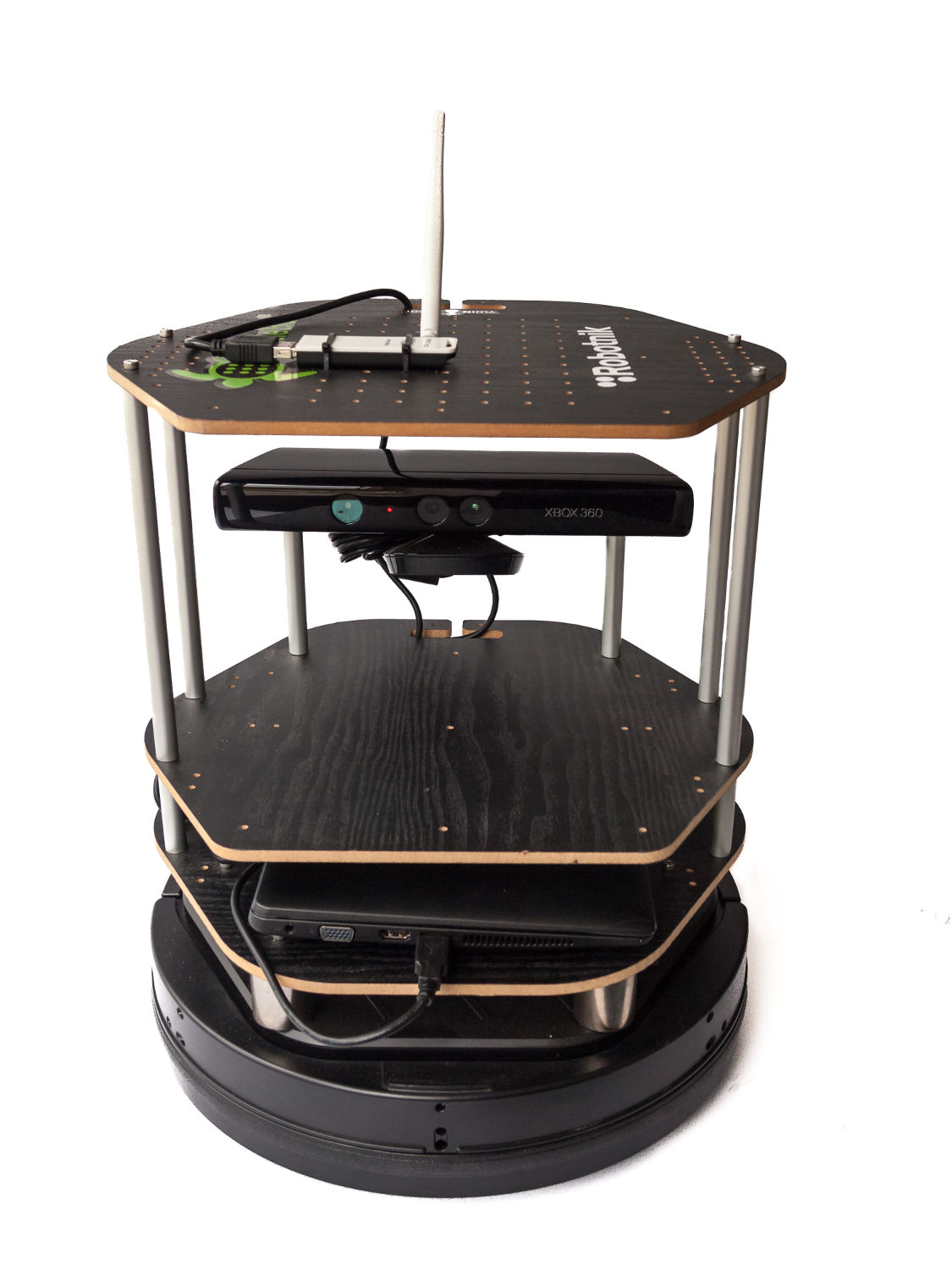
We are using a TurtleBot 2 as a mobile base. The algorithm is implemented as a ROS node using a ROS node for capturing and analyzing the packets We are using the ROS navigation stack for navigation, localization and path planning using the Microsoft Kinect and odometry. The navigation is facilitated by a pre-learned map using OpenSlam’s Gmapping and amcl. As a medium we are using off-the-shelf usb 802.11 wireless dongles and tcpdump/libpcap for capturing packets. For all captured packets sent via the correct MAC-address, RSSI values are extracted from the Radiotap headers. The robot is depicted in fig. 1.

4.2 Internal Models

To limit the computational cost of learning an internal model we chose to learn on a maximum of randomly drawn $10,000$ samples from our data. In the experiments we easily exceed $30,000$ samples. In the following two subsections, section 4.2.1 and section 4.2.2, we give a short overview over the two chosen instantiations of internal models and their implementation as learning strategies.

4.2.1 Local Ridge Regression

Ridge regression is a linear least squares model with a Tikhonov regularization (Tikhonov,, 1943). We use a local version of this by only fitting it to data inside of some radius to have a similar model as used in gradient-based algorithms. We used Ridge regression implemented by scikit-learn (Pedregosa et al.,, 2011) with a local radius of $5\text{\,}\mathrm{m}$ and regularization parameter $\alpha=1.0$. No preprocessing of the data was used.

Even though using this model is similar to the idea of a locally linear Taylor approximation as used in gradient-based methods, it is superior in that it averages over an area, mitigating the effects of small scale fading and noise and in that it is regularized in order to prevent instabilities and overfitting.

4.2.2 Multilayer Perceptron

As a second example of an internal model we chose an MLP with two input neurons, a hidden layer of 100 sigmoid neurons and one linear output neuron. All layers also have access to a bias node. Classic backpropagation with a small momentum term for three epochs was used for learning. We chose to use a fixed number of epochs to limit computational cost. We are not interested in full convergence and cross-validation since the algorithm checks the predictions of the model against real measured data constantly and re-learns the model if the prediction errors surpass a threshold. The network and learning was implemented using PyBrain (Schaul et al.,, 2010). We preprocessed the data to remove the mean and scale it to unit variance because those are assumed by our implementation of artificial neural networks.

5 Experiments

All experiments are performed in a regular office environment with about $20$ different active access points and countless clients in the $2.4\text{\,}\mathrm{GHz}$ band in the test environment. The source node was emitting around $200$ dummy $\text{packets}/s$ which were then captured by the robot.

We also did a complete mapping of the experimental area in terms of RSSI using our setup. The resulting hexagonal histogram is depicted in fig. 2. The bins of the histogram are larger than the wavelength of the wireless signal which means that it represents pure path loss and no interference effects such as small scale fading. We measured an average logarithmic Gaussian noise with a standard deviation of $4\text{\,}\mathrm{dB}$.

Figure 2: Histogram of the example target function $f$ with $422,206$ measurement samples. The position of the target node is depicted as a red star.

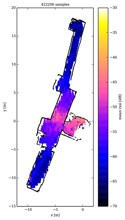
To accurately model small scale fading and other interference effects, a very accurate simulation or even the complete solution of Maxwell’s equations is necessary. This is computationally costly and requires accurate knowledge of material properties of walls etc. Effective models on the other hand are cheaper to calculate but only represent an abstract, stochastic model of the environment. Thus we chose to work directly with real world experiments in order not to lose or miss systematic physical effects such as small scale fading.

Since we performed the experiments during regular office hours, a lot of disturbances such a persons walking, opening and closing doors, changing network load etc. affected the measurements and path planning. Additionally, the algorithm itself is stochastic. Thus, a large number of experiments would have to be conducted to gain statistically sound results. We chose to show some typical experiments instead.

Five typical runs for the two different internal model implementations discussed in section 4.2 are depicted in fig. 3 and fig. 4 respectively. For all experiments the robot starts from the same initial position. The plots show trajectories, points where the model was updated as well as the signal strength as a function of the way travelled.

Figure 3: Experiments done with Ridge regression as an internal model. Top panels shows trajectories on the map of the used office space and lower panels show the history of the measured RSSI values as a function of the distance covered and the moving average over $1\text{\,}\mathrm{m}$. The red star denotes the position of the source. Red circles on the trajectory denote model updates. The initial position of the robot is marked with a red cross.

Figure 4: Experiments done with an MLP as an internal model. Top panels shows trajectories on the map of the used office space and lower panels show the history of the measured RSSI values as a function of the distance covered and the moving average over $1\text{\,}\mathrm{m}$. The red star denotes the position of the source. Red circles on the trajectory denote model updates. The initial position of the robot is marked with a red cross.

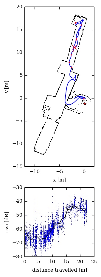
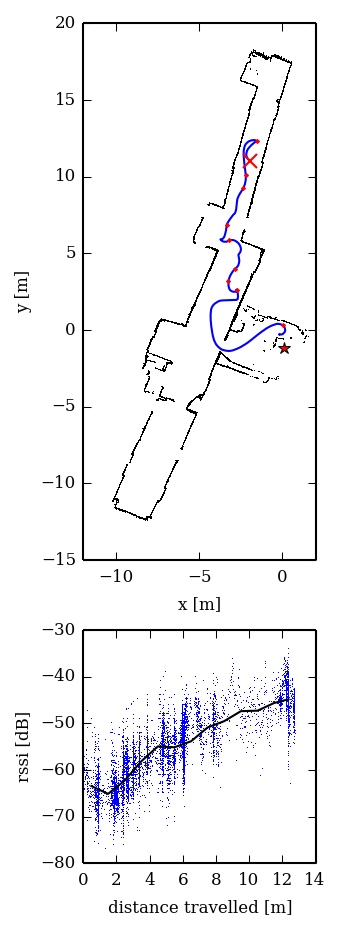
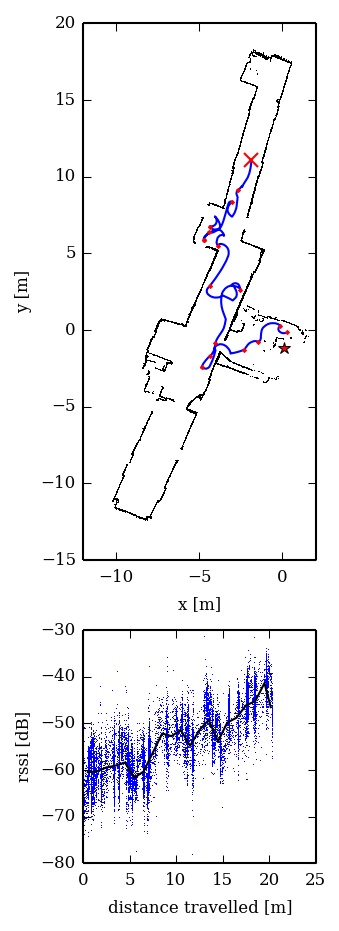
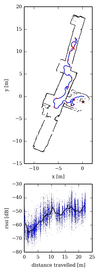
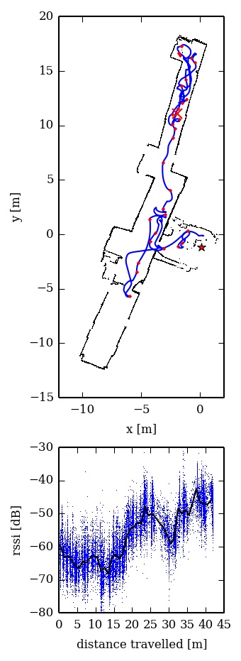
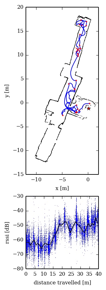
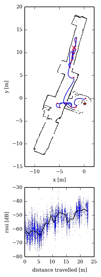
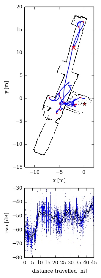
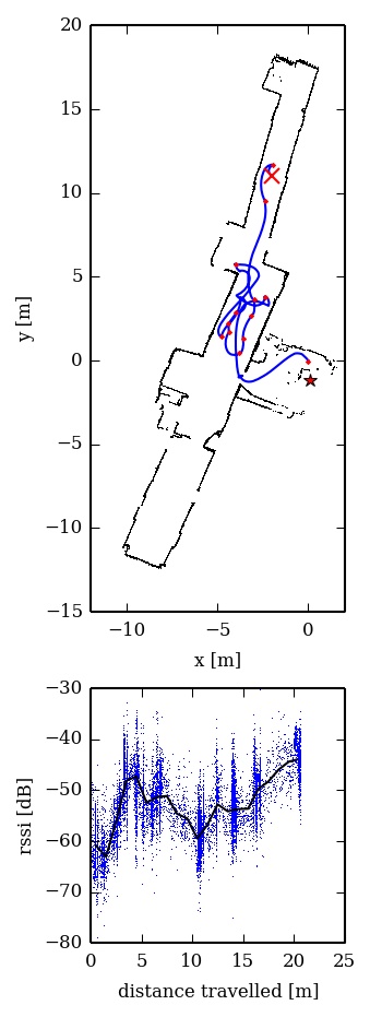
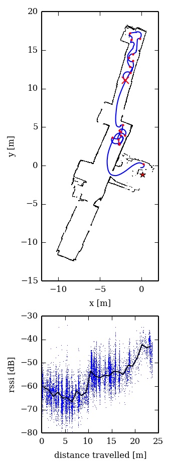
The trajectories show several distinct variations which can shed some light on how the algorithm works. In the beginning of each experiment the robot does not posses any knowledge about the signal strength distribution and starts with an initial random step. For the next five iterations $\epsilon$ is higher than $0.5$ and since the $\epsilon$-steps are novelty driven, the probability of continuing in the same direction as the initial random step is higher than the probability of turning around. Once $\epsilon$ is approaching its final value of $0.1$ and the robot has collected enough samples of the signal strength distribution, it either turns around if it initially went into the wrong direction or it continues on towards the maximum. Once the robot passes the room where the target node is located, it shows a similar behaviour. Either the internal model correctly predicts the position of the target node and the robot directly enters the room or the robot passes by the room but then turns around after the prediction error of the internal model measured against the collected samples passes the error threshold and the model is updated with new samples.

Considering the measurement history of the experiments, it is clear how big of a challenge the task is. Especially far away from the source, the gradients are much smaller than the noise of the measurements. Using finite difference gradient methods would only work for impractically large measurement steps or would lead to very noisy trajectories close to biased random walks. In contrast, both internal models seem to be able to cope with the noise and possible local maxima.

The particular choice of the internal model does not seem to make much of a difference though. This may be due to the simple (and convex) nature of the underlying function, which is essentially the path loss function measured and depicted in fig. 2. The choice of a concrete model might be more important when working with more complex target functions as discussed in section 6. In addition to the two exemplary models shown here, we also tried Support Vector Regression, Kernel Ridge Regression, different other configurations of an MLP, k-Nearest Neighbors Regression and Radius Nearest Neighbor Regression. All representations converged albeit with different convergence speeds. We believe that the choice of the meta-algorithm, i.e., constant model validation and novelty driven $\epsilon$-greedy search, will lead to convergence of the algorithm as long as the particular model is in principle able to represent the target function.

6 Extensions

6.1 Idea und Theory

Figure 5: Example target function $f$ for finding the optimal position to bridge two network nodes as a 1-dimensional simplification. The signal strength of the two nodes with a toy path loss models are plotted on the left y-axis. The target function $f$ is plotted on the right y-axis.

The presented algorithm can readily be extended to solve different tasks by noting that in essence it is just maximizing an unknown function with access to point measurements. The most straightforward extensions in the networking context would thus be to replace signal strength with any other interesting metric like for example Packet-Delivery Ratio (PDR) or Bit-Error Rate (BER). These metrics might be more noisy and contain a lot of local minima but the algorithm is able to cope with that by design.

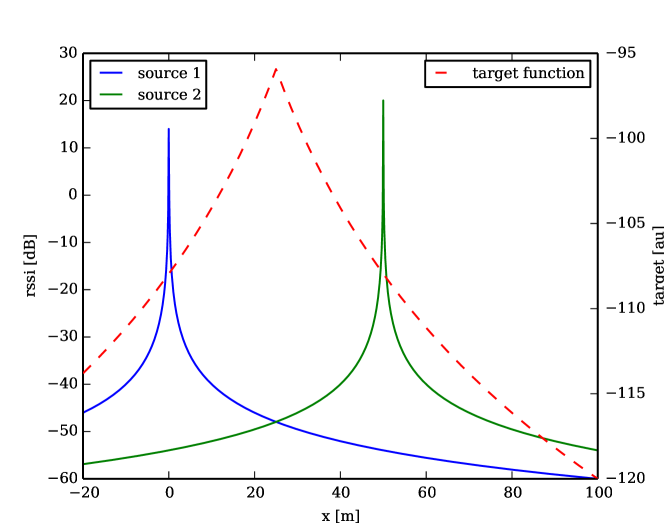
More complex tasks can be easily constructed using compound metrics. As an example we consider the task of bridging two network nodes. Practically, this means moving to the point with the maximal but equal signal strength to both nodes. We construct a single metric fulfilling this criteria using the signal strengths of both nodes using a target function $f$ like

$$f=-\lvert\text{RSSI}_{1}-\text{RSSI}_{2}\rvert-\lvert\text{RSSI}_{1}+\text{RSSI}_{2}\rvert$$

where the indices $1$ and $2$ correspond to both nodes in question. This target function $f$ with toy signal strength path loss functions for both nodes is depicted in fig. 5.

The target function shows a clear maximum at exactly the center between the two source positions, so maximising it leads to maximal and equal signal strengths of both nodes.

This is only a toy example and other task-specific metrics can be designed making this algorithm very versatile in formulating and solving tasks for mobile nodes in wireless networks. A cross-layer approach would be especially interesting. For more complicated target functions, which are probably also more noisy, more complex internal models can be beneficial.

6.2 Experiment

Figure 6: Histogram of the example target function $f$ with $469,108$ measurement samples. The positions of the two nodes to be bridged are depicted as red stars.

Figure 7: The top panel depicts the trajectory of the robot for one experiment using the target function $f$. The initial position of the robot is marked with a red cross. The positions of the two nodes which have to be bridged are depicted as red stars. Model updated are denoted by red points. The lower panel shows the measurements of the target function as a function of travelled distance and the moving average over $1\text{\,}\mathrm{m}$ of the measurements.

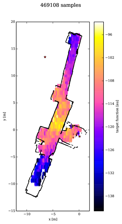
We did exemplary experiments with two nodes and the target function shown above. One of the nodes was the one used for the earlier experiments and the second one was placed in a different office. Both nodes were simple USB wireless adapters dongles sending packets. Again, the experiments were conducted during regular office hours. fig. 6 shows the histogram of the measured values over all experiments conducted. As expected the function has one maximum somewhere between both nodes.

Using the target function $f$ means that the noise of the measurements of both sources are combined following the law of propagation of uncertainty, which yields for the case of the same but independent noise for both nodes and the use of the target function $f$ twice the noise of a single node, which is around $4\text{\,}\mathrm{dB}$. We measured a standard deviation of about $9\text{\,}\mathrm{arb.unit}$ for our experiments which agrees well with the predicted error.

This also means that the magnitude of measured gradients would be less than the noise of the experiment, which means that a gradient descent algorithm would show a behaviour similar to a random walk with drift instead of a noisy gradient descent. Convergence would not be impacted by this high error but convergence speed would be low.

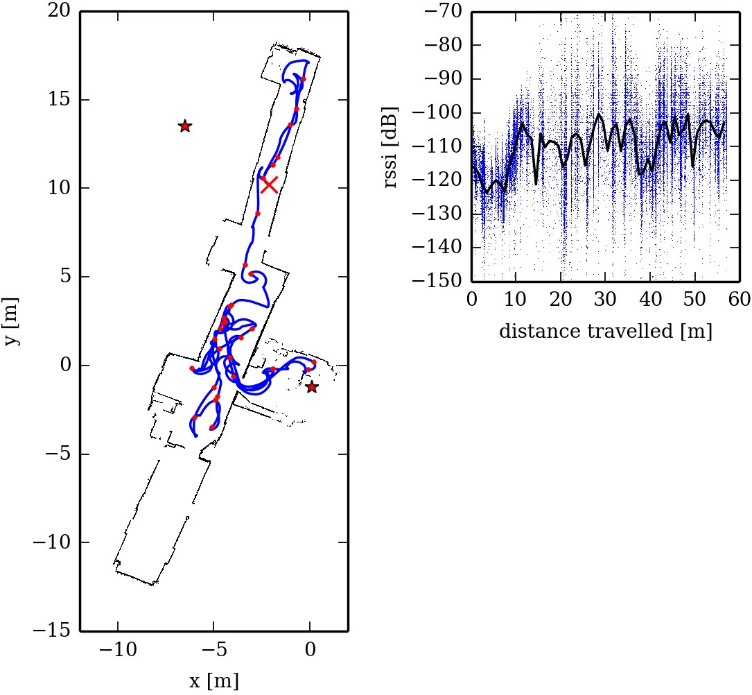
fig. 7 depicts an exemplary experiment. We used an MLP as the internal model with the same parameters as for the single source experiment but we changed the error threshold to $7\text{\,}\mathrm{arb.unit}$ to account for the increased noise. The trajectory of the robot converges to the area of the maximum of fig. 6. The experiment was terminated before a stable maximum was reached because we chose to anneal $\epsilon$ to $0.1$ instead of $0.0$ which means that no fixed position can be reached by design. The magnitude of the noise can be seen in the measurement log of fig. 7.

The behaviour of the algorithm certainly can be improved by tuning parameters but the general idea of testing the internal model predictions against real measurements and refining it when necessary in combination with the $\epsilon$-greedy strategy ensures convergence even without optimized parameters and in spite of very noisy measurements.

7 Conclusions

In this paper we have introduced a class of algorithms to solve a number of tasks related to network robotics, specifically to autonomous mobile network nodes interacting with a wireless network. Beginning with the most basic task of source seeking, the general algorithm has shown to be effective in real world scenarios by a series of experiments with a real physical robot in an office environment. We then showed how this algorithm can be extended to various other tasks, which can be encountered by a mobile network node, such as maximizing the PDR to a certain target node or bridging two network nodes. For the bridging scenario an exemplary experiment has been conducted successfully.

Furthermore, we have given insight into the robotics view on the problem and have discussed the relationship to conventional algorithms. We believe that this discussion can further the field of network robotics in an interdisciplinary manner and can also lead to new insights in other related fields.

References

- Atanasov et al., (2012) Atanasov, N., Le Ny, J., Michael, N., and Pappas, G. J. (2012). Stochastic source seeking in complex environments. In Robotics and Automation (ICRA), 2012 IEEE International Conference on, pages 3013–3018. IEEE.
- Berg and Brown, (1972) Berg, H. C. and Brown, D. A. (1972). Chemotaxis in escherichia coli analysed by three-dimensional tracking. Nature, 239(5374):500–504.
- Blum and Hafner, (2014) Blum, C. and Hafner, V. V. (2014). Gradient-based taxis algorithms for network robotics. arXiv preprint arXiv:1409.7580.
- Braitenberg, (1986) Braitenberg, V. (1986). Vehicles: Experiments in synthetic psychology. MIT press.
- Daniel et al., (2010) Daniel, K., Rohde, S., Goddemeier, N., and Wietfeld, C. (2010). A communication aware steering strategy avoiding self-separation of flying robot swarms. In Intelligent Systems (IS), 2010 5th IEEE International Conference, pages 254–259. IEEE.
- Dantu et al., (2009) Dantu, K., Goyal, P., and Sukhatme, G. (2009). Relative bearing estimation from commodity radios. In Robotics and Automation, 2009. ICRA’09. IEEE International Conference on, pages 3871–3877. IEEE.
- Demiris and Khadhouri, (2006) Demiris, Y. and Khadhouri, B. (2006). Hierarchical attentive multiple models for execution and recognition of actions. Robotics and autonomous systems, 54(5):361–369.
- Derenick et al., (2011) Derenick, J., Fink, J., and Kumar, V. (2011). Localization using ambiguous bearings from radio signal strength. In Intelligent Robots and Systems (IROS), 2011 IEEE/RSJ International Conference on, pages 3248–3253. IEEE.
- Fink and Kumar, (2010) Fink, J. and Kumar, V. (2010). Online methods for radio signal mapping with mobile robots. In Robotics and Automation (ICRA), 2010 IEEE International Conference on, pages 1940–1945. IEEE.
- Han et al., (2009) Han, D., Andersen, D. G., Kaminsky, M., Papagiannaki, K., and Seshan, S. (2009). Access point localization using local signal strength gradient. Passive and Active Network Measurement, pages 99–108.
- Haruno et al., (1999) Haruno, M., Wolpert, D. M., and Kawato, M. (1999). Multiple paired forward-inverse models for human motor learning and control. Advances in neural information processing systems, pages 31–37.
- Hauert et al., (2010) Hauert, S., Leven, S., Zufferey, J.-C., and Floreano, D. (2010). Communication-based swarming for flying robots. In International Workshop on Self-Organized Systems, number LIS-POSTER-2010-001.
- Little and Sommer, (2013) Little, D. Y. and Sommer, F. T. (2013). Learning and exploration in action-perception loops. Frontiers in Neural Circuits, 7(37).
- Mattern and Floerkemeier, (2010) Mattern, F. and Floerkemeier, C. (2010). From the internet of computers to the internet of things. In From active data management to event-based systems and more, pages 242–259. Springer.
- Paul et al., (2011) Paul, L. Y., Twigg, J. N., and Sadler, B. M. (2011). Radio signal strength tracking and control for robotic networks. SPIE Defense, Security, and Sensing, pages 803116–803116.
- Pedregosa et al., (2011) Pedregosa, F., Varoquaux, G., Gramfort, A., Michel, V., Thirion, B., Grisel, O., Blondel, M., Prettenhofer, P., Weiss, R., Dubourg, V., Vanderplas, J., Passos, A., Cournapeau, D., Brucher, M., Perrot, M., and Duchesnay, E. (2011). Scikit-learn: Machine learning in Python. Journal of Machine Learning Research, 12:2825–2830.
- Schaul et al., (2010) Schaul, T., Bayer, J., Wierstra, D., Sun, Y., Felder, M., Sehnke, F., Rückstieß, T., and Schmidhuber, J. (2010). PyBrain. Journal of Machine Learning Research, 11:743–746.
- Schillaci et al., (2012) Schillaci, G., Lara, B., and Hafner, V. V. (2012). Internal simulations for behaviour selection and recognition. In Salah, A. A., del Solar, J. R., Mericli, C., and Oudeyer, P.-Y., editors, HBU, volume 7559 of Lecture Notes in Computer Science, pages 148–160. Springer.
- Sutton and Barto, (1998) Sutton, R. S. and Barto, A. G. (1998). Introduction to reinforcement learning. MIT Press.
- Tikhonov, (1943) Tikhonov, A. N. (1943). On the stability of inverse problems. In Dokl. Akad. Nauk SSSR, volume 39, pages 195–198.
- Twigg et al., (2012) Twigg, J. N., Fink, J. R., Yu, P., and Sadler, B. M. (2012). Rss gradient-assisted frontier exploration and radio source localization. In Robotics and Automation (ICRA), 2012 IEEE International Conference on, pages 889–895. IEEE.
- Wadhwa et al., (2011) Wadhwa, A., Madhow, U., Hespanha, J., and Sadler, B. M. (2011). Following an rf trail to its source. In Communication, Control, and Computing (Allerton), 2011 49th Annual Allerton Conference on, pages 580–587. IEEE.
- Wolpert et al., (2011) Wolpert, D. M., Diedrichsen, J., and Flanagan, J. R. (2011). Principles of sensorimotor learning. Nature Reviews Neuroscience, 12(12):739–751.
- Wolpert et al., (2003) Wolpert, D. M., Doya, K., and Kawato, M. (2003). A unifying computational framework for motor control and social interaction. Philosophical Transactions of the Royal Society of London. Series B: Biological Sciences, 358(1431):593–602.
- PDR
- Packet-Delivery Ratio
- BER
- Bit-Error Rate
- RSSI
- Received Signal Strength Indicator