Emission-rotation correlation in pulsars: new discoveries with optimal techniques

Abstract

Pulsars are known to display short-term variability. Recently, examples of longer-term emission variability have emerged that are often correlated with changes in the rotational properties of the pulsar. To further illuminate this relationship, we have developed techniques to identify emission and rotation variability in pulsar data, and determine correlations between the two. Individual observations may be too noisy to identify subtle changes in the pulse profile. We use Gaussian process (GP) regression to model noisy observations and produce a continuous map of pulse profile variability. Generally, multiple observing epochs are required to obtain the pulsar spin frequency derivative ($\dot{\nu}$). GP regression is, therefore, also used to obtain $\dot{\nu}$, under the hypothesis that pulsar timing noise is primarily caused by unmodelled changes in $\dot{\nu}$. Our techniques distinguish between two types of variability: changes in the total flux density versus changes in the pulse shape. We have applied these techniques to 168 pulsars observed by the Parkes radio telescope, and see that although variations in flux density are ubiquitous, substantial changes in the shape of the pulse profile are rare. We reproduce previously published results and present examples of profile shape changing in seven pulsars; in particular, a clear new example of correlated changes in profile shape and rotation is found in PSR J1602$-$5100. In the shape changing pulsars, a more complex picture than the previously proposed two state model emerges. We conclude that our simple assumption that all timing noise can be interpreted as $\dot{\nu}$ variability is insufficient to explain our dataset.

1 Introduction

Pulsars are employed as precision timing tools, due to the stability of their emission and of their rotation. The average radio pulse shape (known as the pulse profile) has traditionally been thought to remain steady over decades, and extreme rotational stability results from the high angular momentum of a rapidly spinning, dense star. Pulsar stability exists even in the presence of nulling and mode-changing: short-term emission variations that were first observed soon after the discovery of pulsars (Backer, 1970a, b). These discontinuous changes occur on time-scales ranging from a few pulse periods to hours and days (Wang et al., 2007). Mode-changing pulsars switch between two or more quasi-stable states, while nulling is thought to be an extreme form of mode-changing, with one state showing no or low emission. These effects aside, the pulse profile has long been considered a stable characteristic of each pulsar. The last decade, however, has witnessed a number of counter-examples to this perceived stability.
A small, emerging population of radio pulsars have shown pulse profile changes on time-scales of months to years (e.g. Lyne et al., 2010). These changes are often accompanied by timing noise, a term given to the unexplained, systematic deviation from the modelled rotational behaviour of a pulsar, often seen in younger pulsars. Although common, the causes of timing noise are poorly understood. One possibility is that timing noise is due (at least in part) to unmodelled variability in the spin-frequency derivative or spindown rate ($\dot{\nu}$) of the pulsar. Under this assumption, timing noise can be modelled as a time-variable $\dot{\nu}$, which leads to the observed correlation between pulse profile and $\dot{\nu}$ variations (Lyne et al., 2010; Keith et al., 2013; Brook et al., 2013).
An extreme example of correlated emission and rotation variability is observed in a group of intermittent pulsars (Kramer et al., 2006; Camilo et al., 2012; Lorimer et al., 2012). Such objects cycle quasi-periodically between intervals in which the pulsar is emitting normally, and those in which no emission is detected. This cyclic behaviour occurs on time-scales of months to years. All known intermittent pulsars lose rotational energy at a much higher rate when their emission is visible; one possible explanation is changing magnetospheric currents (Kramer et al., 2006).
Neutron star glitches, characterised by a discrete increase and gradual relaxation of the rotational frequency, have also recently been linked to pulse profile variability in radio pulsars (Weltevrede et al., 2011; Keith et al., 2013), providing additional links between emission and rotation. Furthermore, examples of glitches and irregular spindown properties associated with emission variability, have been seen in magnetars (Woods & Thompson, 2006), where dramatic profile changes, related to changes in the magnetic field structure have been observed both in X-rays and radio (e.g. Camilo et al., 2007).
Any unmodelled variability is detrimental to experiments that rely on precision pulsar timing, such as the search for gravitational waves using pulsar timing arrays. The observed correlation between timing and pulse profile variability suggests that this information may be used to improve the precision of pulsar timing experiments. In addition, it is revealing a new type of phenomenology that may hold information on the interiors and environments of pulsars.
In this work we make the assumption that all unmodelled timing variations can be attributed to changes in $\dot{\nu}$. Under this assumption we investigate the pulse profile and timing variability in a large number of pulsars to identify any correlation. We have analysed data from 168 pulsars that have been monitored for up to eight years by the Parkes radio telescope. These objects represent a population of young, energetic pulsars, known to show the most timing noise, thus offering possibilities to test the above hypothesis. The only exception is PSR J0738$-$4042, which is monitored due to its known variable behaviour (Brook et al., 2013). We present nine interesting examples of pulsar variability in this paper, including PSR J0738$-$4042 and two pulsars previously studied in Lyne et al. (2010).
In Section 2, we detail the observations. Section 3 describes the data analysis techniques used to detect both emission and rotational variability. The results from nine pulsars are presented in Section 4, followed by a discussion and conclusions in sections 5 and 6 respectively.

2 Observations

Since 2007, 168 pulsars have been observed on a roughly monthly basis at 1369 MHz with the Parkes radio telescope and the Multibeam receiver as part of the Fermi timing programme (Weltevrede et al., 2010). The data were recorded with one of the Parkes Digital Filterbank systems (PDFB1/2/3/4) with a total bandwidth of 256 MHz in 1024 frequency channels. Radio frequency interference was removed using median-filtering in the frequency domain and then manually excising bad sub-integrations. Flux densities have been calibrated by comparison to the continuum radio source 3C 218. The data were then polarization-calibrated for both differential gain and phase, and for cross coupling of the receiver. The MEM method based on long observations of 0437-4715 was used to correct for cross coupling (van Straten, 2004). Flux calibrations from Hydra A were used to further correct the bandpass. After this calibration, profiles were formed of total intensity (Stokes parameter I), and averaged over time and frequency. The profiles were cross-correlated with templates with a high signal-to-noise ratio (S/N) to obtain times of arrival (TOAs), using standard techniques for pulsar timing (Hobbs et al., 2006). The template used to calculate the TOAs is noiseless, generated iteratively from a set of von Mises functions in order to represent the profile, formed from the summation of all observations.

3 Data Analysis

The objective of the data analysis is to model the variability of pulse profiles that have been sampled at irregular intervals, and compute the $\dot{\nu}$ timeseries for each pulsar. We have developed a technique that models the pulse profile data as a function of time, allowing us to interpolate between the epochs of observation. This builds on work by Brook et al. (2013). This process also allows better visualisation of sparsely sampled data. Irregular sampling again raises difficulties in the calculation of $\dot{\nu}$, which we have also addressed using similar inference techniques. These techniques are based on Gaussian process (GP) non-parametric modelling, details of which are provided in the following.

3.1 Pulse profile variability maps

We use the term variability map to describe an interpolated plot that maps the differences (i.e. the profile residuals) between the pulse profile at each observation and a constant model. The model is taken to be the median of all observed profiles in a dataset. Panels A and B of Figure 3 are examples of variability maps. Before the observed pulse profiles can be compared with the constant model, we process them to ensure the off-pulse baseline is centred on zero. Some observations are considered unreliable and excluded from further analysis. A pulse profile is excluded using the following empirical rule which has been found to perform well in rejecting spurious observations: if the standard deviation of the off-pulse region is greater than a factor of two larger than the median value taken from the off-pulse regions across all epochs. Observations are also removed manually if they show extreme and isolated profile deviations that can likely be attributed to instrumental failure.
All pulse profiles originally consist of 1024 phase bins across the pulse period. If S/N is low for any pulsar then pulse profile variations can become difficult to detect. In cases where the profile with the highest S/N in a pulsar dataset has a peak value less than 20 times the standard deviation of the off-pulse noise, the S/N is increased by reducing the number of phase bins to 128. The individual profiles are aligned by cross-correlation with the median over all epochs. Using the timing information to align the profiles is not possible, given the amount of timing noise in the data. Aligning the profiles is essential for the modelling that follows, as the timeseries of each pulse phase bin is modelled independently. In the few observations where large profile deviations occur, it is possible that the alignment may be slightly biased in that direction, however, all observations have been individually inspected to exclude the possibility that this effect plays an important role.
We use variability maps to monitor two types of profile variability: changes in the flux density across the whole pulse profile, and changes in the relative flux density of profile components, i.e. shape variations. In this paper, we primarily focus on the latter, as large flux density variations are observed in most of the pulsar data analysed in this work, and are thought to be primarily attributable to the effects of refractive scintillation. To uncover the less common pulse profile shape changes, we normalise all observations by the mean on-pulse flux density.
Two median profiles were calculated for each pulsar dataset: one for the normalised data described above and one for the non-normalised, flux calibrated data. The relevant median profile was then subtracted from each observation, leaving the profile residual (following Brook et al., 2013). For each of the pulse profile phase bins, we compute a GP regression model that best describes the profile residuals (Rasmussen & Williams, 2006; Roberts et al., 2012), which we observe to often have sharp turnover features. The covariance function chosen for this analysis, therefore, employs a kernel from the Matern class:

$$k(x_{i},x_{j})=\sigma_{f}^{2}\frac{2^{1-\mu}}{\Gamma(\mu)}\left(\frac{\sqrt{2\mu}d}{\lambda}\right)^{\mu}K_{\mu}\left(\frac{\sqrt{2\mu}d}{\lambda}\right),$$ (1)

where $\Gamma$ is the gamma function, $K_{\mu}$ is a modified Bessel function, d is the distance $|x_{i}-x_{j}|$ between any two epochs (training points), $\sigma_{f}^{2}$ is the maximum allowable covariance, and $\lambda$ is the characteristic lengthscale, i.e. a parameter which reflects how significantly the distance between $x_{i}$ and $x_{j}$ affects $k(x_{i},x_{j})$. The positive covariance parameter $\mu$ was chosen to be 3/2 to provide a level of smoothness and flexibility to the covariance function that is suitable for the kind of trends we are trying to model (Rasmussen & Williams, 2006):

$$k_{3/2}(x_{i},x_{j})=\sigma_{f}^{2}\left(1+\frac{\sqrt{3}d}{\lambda}\right)\exp\left(-\frac{\sqrt{3}d}{\lambda}\right).$$ (2)

This Matern covariance kernel was combined with a white noise kernel $\sigma_{n}^{2}\delta_{x_{i}x_{j}}$ to model the uncertainty in the profile data, where $\delta_{x_{i}x_{j}}$ is the Kronecker delta function and $\sigma_{n}$ is the standard deviation of the noise term in the model. The choice of hyperparameters $\theta$ ($\sigma_{f}$, $\lambda$, $\sigma_{n}$) for the covariance function employed by the GP, is made by maximising log $p(\textbf{y}|\textbf{x},\theta)$. In this process we constrain the lengthscale $\lambda$ between 30 and 300 days, which we find to result in the models best representing the data. The GP takes the training points (the observed data; $x_{i}$ and corresponding $y_{i}$) and calculates test points, i.e. the most likely value $y_{*}$ for any value $x_{*}$, and its variance:

$$y_{*}=K_{*}K_{ij}^{-1}\textbf{y}$$ (3)

$$var(y_{*})=K_{**}-K_{*}K_{ij}^{-1}K_{*}^{T},$$ (4)

where $K_{ij}$ is a covariance matrix with components $k(x_{i},x_{j})$ over all training points, $K_{*}$ is a matrix which reflects covariance between a test point and the training points and has components $k(x_{*},x_{i})$. The covariance of a test point $K_{**}=k(x_{*},x_{*})$.
A GP regression model is produced for all phase bins, with test points computed at one day intervals. These models are then combined to produce a continuous variability map, which highlights deviations across the pulse profile and across the data span (e.g. Panels A and B of Figure 3).

3.2 Rotational Variability

As mentioned in the introduction, we are testing the hypothesis that all unmodelled variations in pulsar timing can be explained as time-variable changes in $\dot{\nu}$. In order to calculate a time variable $\dot{\nu}$, we use the timing residuals, which are the differences between observed pulse TOAs and a timing model with a constant set of parameters (e.g. pulse period, period derivative, position, proper motion). The model is optimised by using a least-squares-fitting procedure to minimize the timing residuals.
In the case of a pulsar with time variable $\dot{\nu}$, a timing model with constant parameters will result in systematic timing residuals. Keith et al. (2013) describe how the second derivative of these timing residuals represents a $\dot{\nu}$ term that is additional to the timing model. We have developed a new technique which employs GP regression to analytically model the timing residuals, allowing us to produce a continuous function representing $\dot{\nu}$ for each pulsar. The Keith et al. calculation is based on the interpolation technique of Deng et al. (2012), who use a generalised Wiener filter as a maximum likelihood estimator for pulsar timing residuals. This technique can be considered a special case of our fully Bayesian inference method (Rasmussen & Williams, 2006). While the Deng et al. technique provides a means to smoothly interpolate between residuals, it does not provide uncertainties for the interpolated data. This makes it non-trivial to obtain useful uncertainty estimates of the derivative values of a model produced by maximum likelihood estimation; Keith et al. find the second derivative of their timing residual interpolation by numerically differentiating twice. In contrast, Gaussian process regression allows us to analytically model the second derivative directly from the timing residuals, with associated fully Bayesian error estimation. GP regression does not require regularly evenly sampled data.
For this technique, we use a squared exponential covariance kernel because it is infinitely differentiable:

$$k(x_{i},x_{j})=\sigma_{f}^{2}\exp\left(\frac{-d^{2}}{2\lambda^{2}}\right),$$ (5)

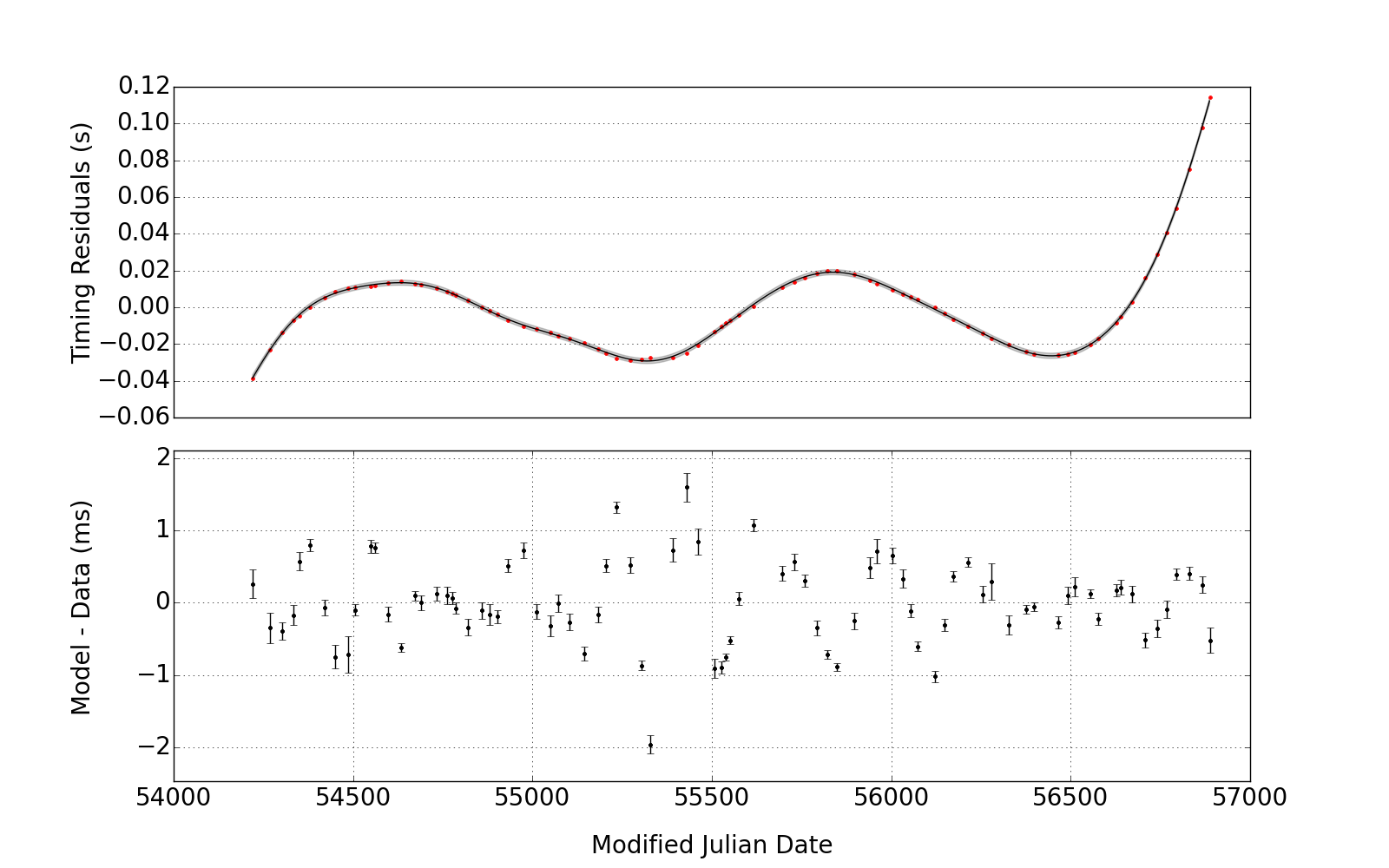
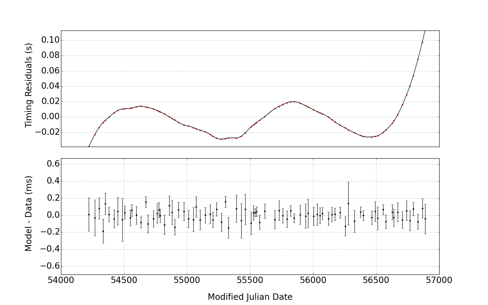
along with the white noise kernel. When observing how well the GP model and optimised covariance hyperparameters $\theta$ fit to the timing residuals, however, we noticed that one kernel was not always sufficient to describe them. Adding a second squared exponential kernel to the covariance function models the timing residuals more accurately in all but two of the nine pulsars detailed in this work. As an example, Figures 1 and 2 show the timing residuals of PSR J0940$-$5428 fitted with a GP using one and two kernels respectively. The discrepancies between the data and the model are also shown. The error bars in the lower panel represent $\sigma_{TOA}$, the uncertainty in the TOA measurement. It is clear that the single kernel model in Figure 1 systematically deviates from the TOA measurements, whereas the same panel of Figure 2 reveals a near perfect fit.
To calculate $\dot{\nu}$, we optimised the hyperparameters $\theta$, as described in Section 3.1. Whether the covariance function contains one or two kernels, the value of each lengthscale was restricted to between 30 and 1000 days; all other parameters were unbounded. The optimised covariance hyperparameters $\theta$ were then carried forward to calculate the second derivative of the GP regression model of the timing residuals; following Holsclaw et al. (2013), the second derivative of a GP model can be estimated using the second derivative of the covariance kernel. In the case of the squared exponential kernel:

$$k^{{}^{\prime\prime}}(x_{i},x_{j})=\frac{\sigma_{f}^{2}}{\lambda^{2}}\exp\left(\frac{-d^{2}}{2\lambda^{2}}\right)\left(1-\frac{d^{2}}{\lambda^{2}}\right).$$ (6)

The second derivative of the GP model:

$$\frac{d^{2}y_{*}}{dx^{2}}=K^{{}^{\prime\prime}}_{*}K_{ij}^{-1}\textbf{y}.$$ (7)

The value of $\dot{\nu}$ can trivially be shown to be:

$$\nu\frac{d^{2}y_{*}}{dx^{2}}.$$ (8)

The variance of this method is given by:

$$var\left(\frac{d^{2}y_{*}}{dx^{2}}\right)=A-K^{{}^{\prime\prime}}_{*}K_{ij}^{-1}K^{{}^{\prime\prime}}_{*},$$ (9)

where $A$ is the diagonal terms of $k^{{}^{\prime\prime\prime\prime}}(x_{i},x_{j})$, which gives:

$$\frac{3\sigma_{f}^{2}}{\lambda^{4}}$$ (10)

in the case of one covariance kernel. When plotting the $\dot{\nu}$ model, test points were calculated only for days on which the pulsar was observed.

Figure 1: The timing residuals and GP model for PSR J0940$-$5428 using one kernel in the covariance function. Top panel: The red points are the timing residuals. The black trace shows the GP model, which has a covariance function that employs one kernel with a lengthscale of 276 days. The shaded 2$\sigma$ uncertainty region indicates the range of GP models that can describe the data. Bottom panel: The GP model minus the timing residuals at the epochs of the observations. The structure seen here implies an ill-fitting model that does not account for the short-term periodic behaviour seen in the data. The uncertainty in bottom panel is that of the timing residuals.

Figure 2: The timing residuals and GP model for PSR J0940$-$5428. As Figure 1, but employing two kernels in the covariance function; the lengthscales are 60 days and 471 days. The lack of structure in the bottom panel suggests a well-fitting model and justifies the number of kernels and optimised parameters used in the covariance function.

PSR J	PSR B	$\nu$ (s-1)	$\dot{\nu}$ (s-2)	DM (cm-3pc)	Age (Yr)	$B_{surface}$ (G)	$\dot{E}$ (Js${}^{-1})$
0738$-$4042	0736$-$40	2.667	$-1.150\times 10^{-14}$	160.8	$3.68\times 10^{6}$	$7.88\times 10^{11}$	$1.2\times 10^{33}$
0742$-$2822	0740$-$28	5.997	$-6.049\times 10^{-13}$	73.782	$1.57\times 10^{5}$	$1.69\times 10^{12}$	$1.4\times 10^{35}$
0908$-$4913	0906-49	9.367	$-1.329\times 10^{-12}$	180.37	$1.12\times 10^{5}$	$1.29\times 10^{12}$	$4.9\times 10^{35}$
0940$-$5428	$-$	11.423	$-4.289\times 10^{-12}$	134.5	$4.22\times 10^{4}$	$1.72\times 10^{12}$	$1.9\times 10^{36}$
1105$-$6107	$-$	15.825	$-3.963\times 10^{-12}$	271.01	$6.33\times 10^{4}$	$1.01\times 10^{12}$	$2.5\times 10^{36}$
1359$-$6038	1356$-$60	7.843	$-3.899\times 10^{-13}$	293.71	$3.19\times 10^{5}$	$9.10\times 10^{11}$	$1.2\times 10^{35}$
1600$-$5044	1557$-$50	5.192	$-1.365\times 10^{-13}$	260.56	$6.03\times 10^{5}$	$9.99\times 10^{11}$	$2.8\times 10^{34}$
1602$-$5100	1558$-$50	1.157	$-9.316\times 10^{-14}$	170.93	$1.97\times 10^{5}$	$7.85\times 10^{12}$	$4.3\times 10^{33}$
1830$-$1059	1828$-$11	2.469	$-3.659\times 10^{-13}$	161.50	$1.07\times 10^{5}$	$4.99\times 10^{12}$	$3.6\times 10^{34}$

Table 1: Properties of the pulsars showing notable variability.

Pulsar	Max. Cov.	Len.	Noise RMS	Max. Cov. i	Len. i	Max. Cov. ii	Len. ii	Noise RMS	Mean TOA
	1 Kernel	1 Kernel	1 Kernel	2 Kernels	2 Kernels	2 Kernels	2 Kernels	2 Kernels	RMS
	(Secs.)	(Days)	(Secs.)	(Secs.)	(Days)	(Secs.)	(Days)	(Secs.)	(Secs.)
J0738$-$4042	$4.0\times 10^{-3}$	321.9	$1.3\times 10^{-4}$	$4.0\times 10^{-6}$	185.6	$1.7\times 10^{-2}$	893.0	$1.3\times 10^{-4}$	$2.1\times 10^{-5}$
J0742$-$2822	$3.7\times 10^{-2}$	121.4	$2.7\times 10^{-4}$	$3.6\times 10^{-1}$	633.4	$2.2\times 10^{-5}$	59.5	$1.7\times 10^{-4}$	$1.1\times 10^{-5}$
J0908$-$4913	$6.1\times 10^{-5}$	125.1	$8.3\times 10^{-5}$	$6.0\times 10^{-7}$	73.0	$1.2\times 10^{-4}$	229.6	$6.5\times 10^{-5}$	$2.4\times 10^{-6}$
J0940$-$5428	$6.3\times 10^{-3}$	275.5	$6.5\times 10^{-4}$	$3.1\times 10^{-2}$	471.3	$2.2\times 10^{-6}$	59.5	$1.1\times 10^{-4}$	$1.1\times 10^{-4}$
J1105$-$6107	$6.1\times 10^{-4}$	120.4	$6.0\times 10^{-4}$	$2.7\times 10^{-3}$	234.3	$2.7\times 10^{-6}$	51.4	$4.7\times 10^{-4}$	$3.1\times 10^{-5}$
J1359$-$6038	$8.4\times 10^{-4}$	233.6	$6.3\times 10^{-5}$	$9.5\times 10^{-7}$	124.0	$1.2\times 10^{-2}$	780.9	$4.7\times 10^{-5}$	$5.0\times 10^{-6}$
J1600$-$5044	$1.6\times 10^{-4}$	395.2	$1.2\times 10^{-4}$	$5.6\times 10^{-7}$	118.0	$2.4\times 10^{-4}$	615.2	$6.0\times 10^{-5}$	$4.4\times 10^{-6}$
J1602$-$5100	$2.2\times 10^{-1}$	166.3	$3.0\times 10^{-4}$	$4.7\times 10^{-5}$	95.8	$5.6\times 10^{+0}$	506.9	$2.4\times 10^{-4}$	$2.2\times 10^{-5}$
J1830$-$1059	$1.1\times 10^{-3}$	108.5	$4.8\times 10^{-4}$	$2.1\times 10^{-5}$	61.8	$1.9\times 10^{-3}$	227.9	$3.4\times 10^{-4}$	$3.8\times 10^{-5}$

Table 2: The optimised parameters (maximum covariance, lengthscale and noise rms) for a covariance function with one and two kernels, along with the mean TOA rms for each pulsar. An underlined pulsar name indicates that one kernel was used to calculate $\dot{\nu}$. The $\dot{\nu}$ model for all other pulsars was produced using two kernels.

3.3 Correlation maps

Lyne et al. (2010) show a correlation between $\dot{\nu}$ and various metrics of profile shape. In order to understand which regions of the profile may be correlated and whether changes are coincident or occur with a lag, we calculate Spearman’s rank correlation coefficient (SRCC) between the timeseries of $\dot{\nu}$ and of the profile residuals in each phase bin of the pulse profile. We choose SRCC, as it is a measure of the monotonic relationship between the variables, yet linearity is not required.
We apply a lag between each pair of timeseries, up to 500 days in both directions and calculate how SRCC changes. The result is a correlation map for each pulsar (e.g. Panel C of Figure 4). In these maps, we can identify regions of the pulse profile that show most correlation with $\dot{\nu}$, and gain information about the temporal relationship between the two timeseries.
To permit the correlation calculations, we require the two timeseries to be sampled at the same rate. The GP model of the profile residuals provides a value at daily intervals. We, therefore, produce $\dot{\nu}$ models (as described in Section 3.2) which are also sampled at one day intervals.
SRCC is only calculated for the pulse phase bins that lie within the on-pulse region. We have defined this to be the region where the flux density of the median pulse profile of a dataset is greater than 1/30 of its peak value.

4 Results

We have applied the techniques described in Section 3 to data from 168 pulsars observed by the Parkes radio telescope. In the following, we first show results from pulsars with previously documented variability. We then present new examples, discovered using our techniques. Finally, we comment on the remainder of the pulsars in the dataset.

4.1 Known Variable Pulsars

4.1.1 PSR J0738$-$4042 (B0736$-$40)

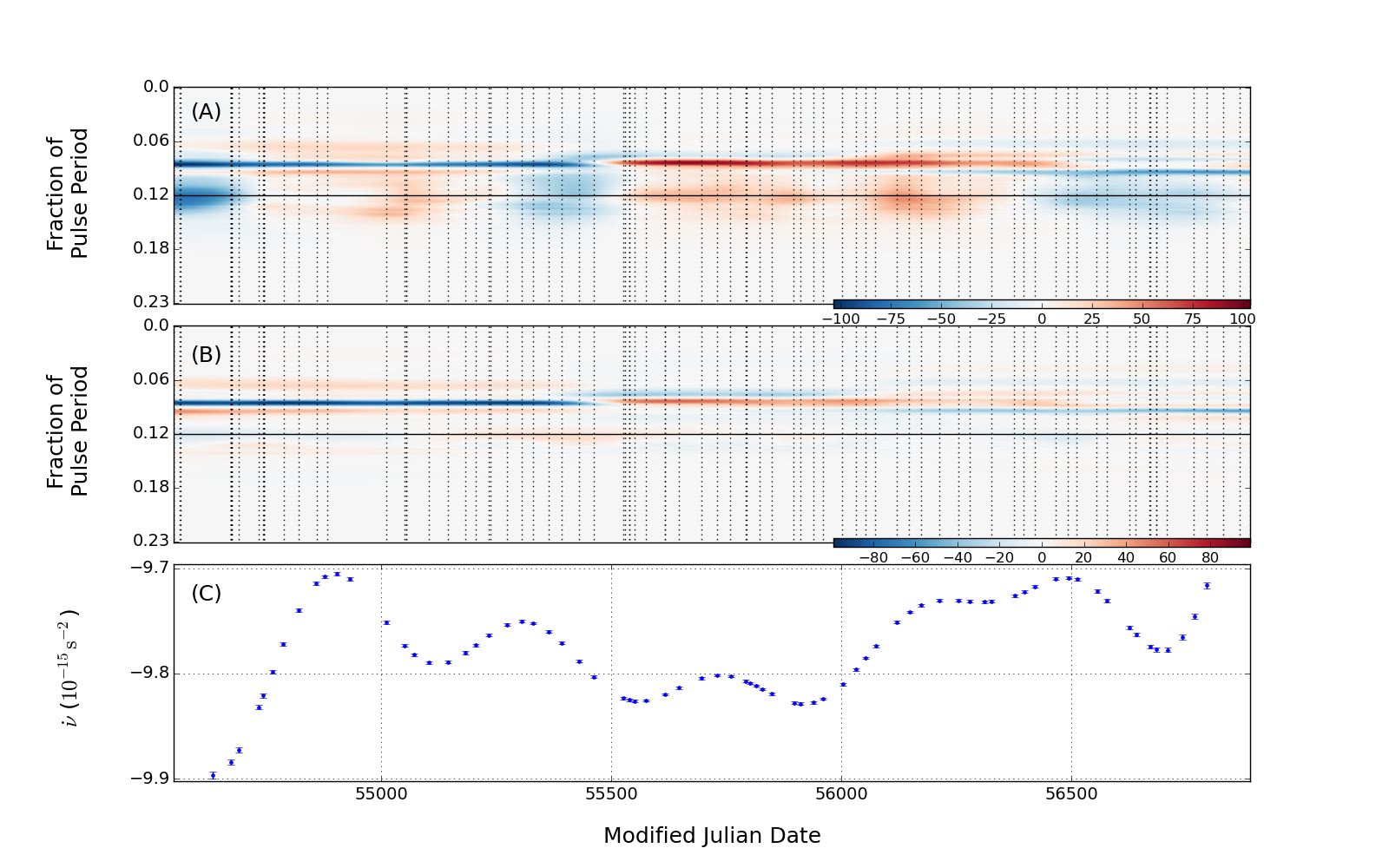
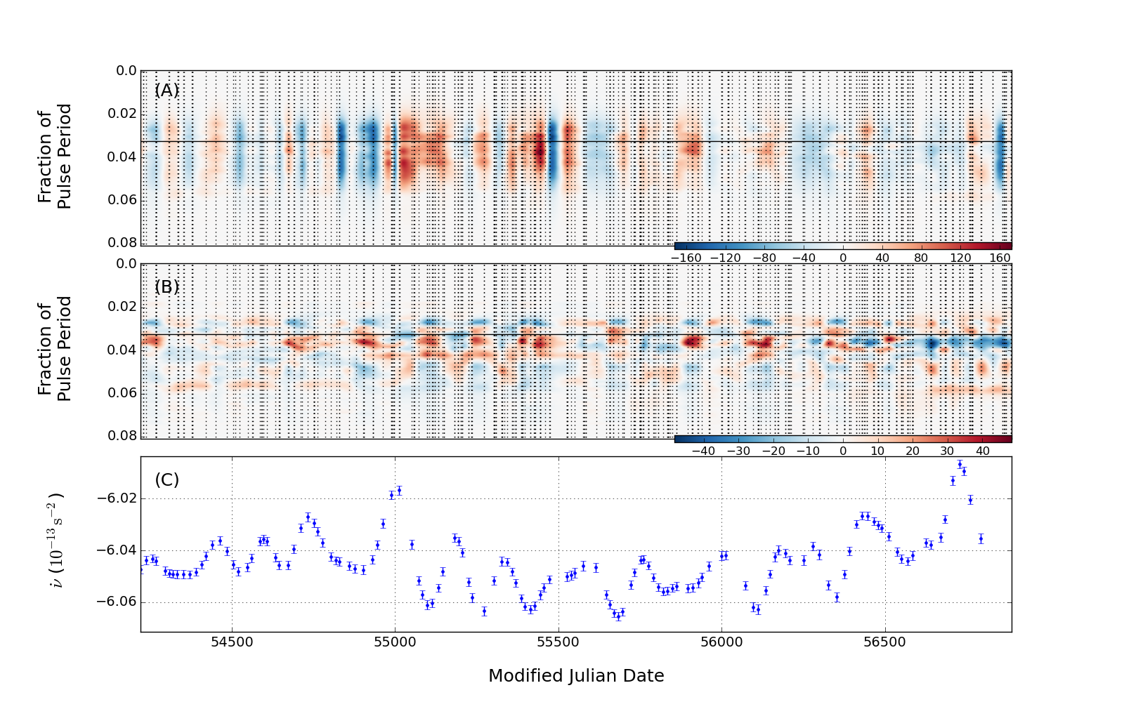
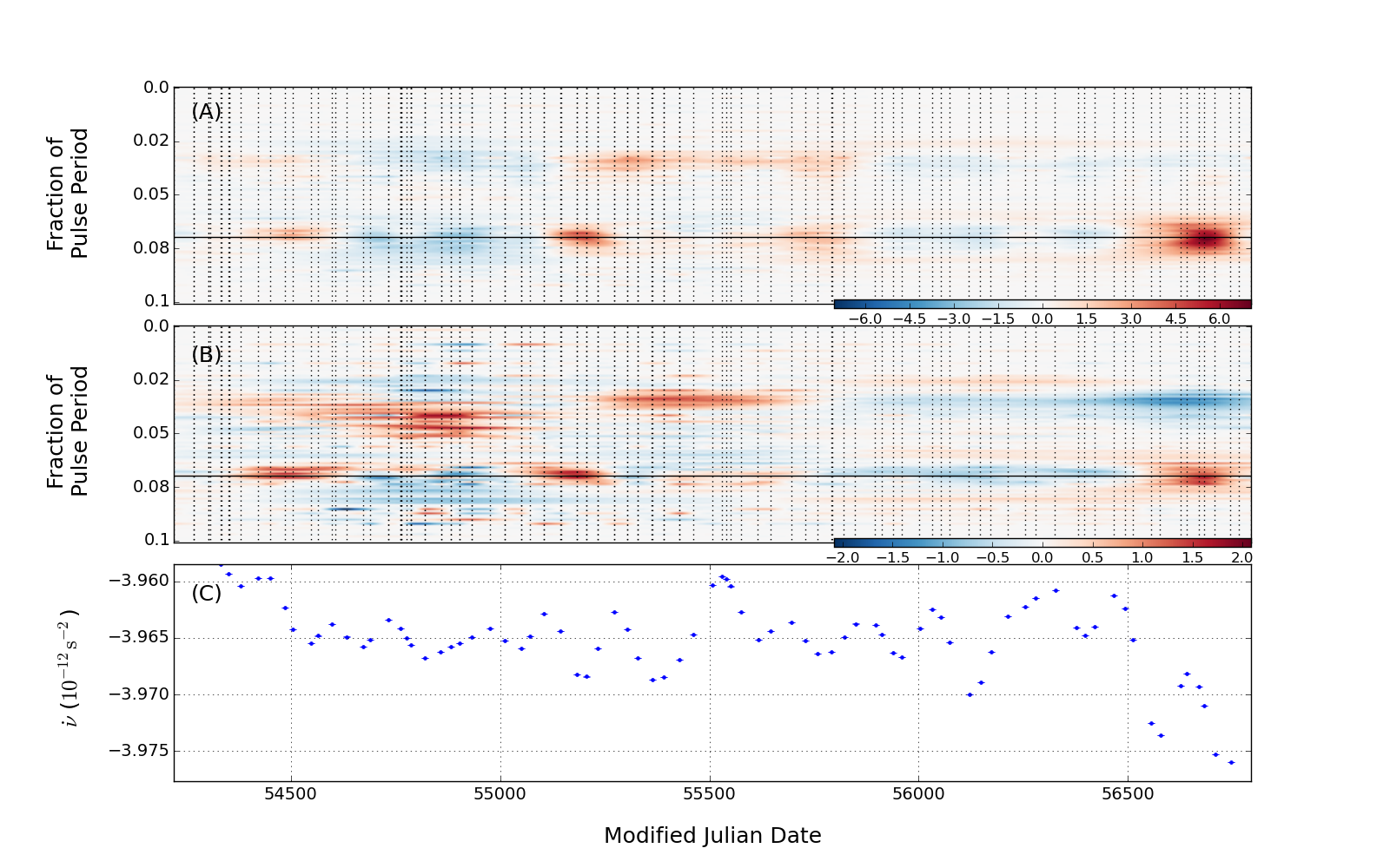
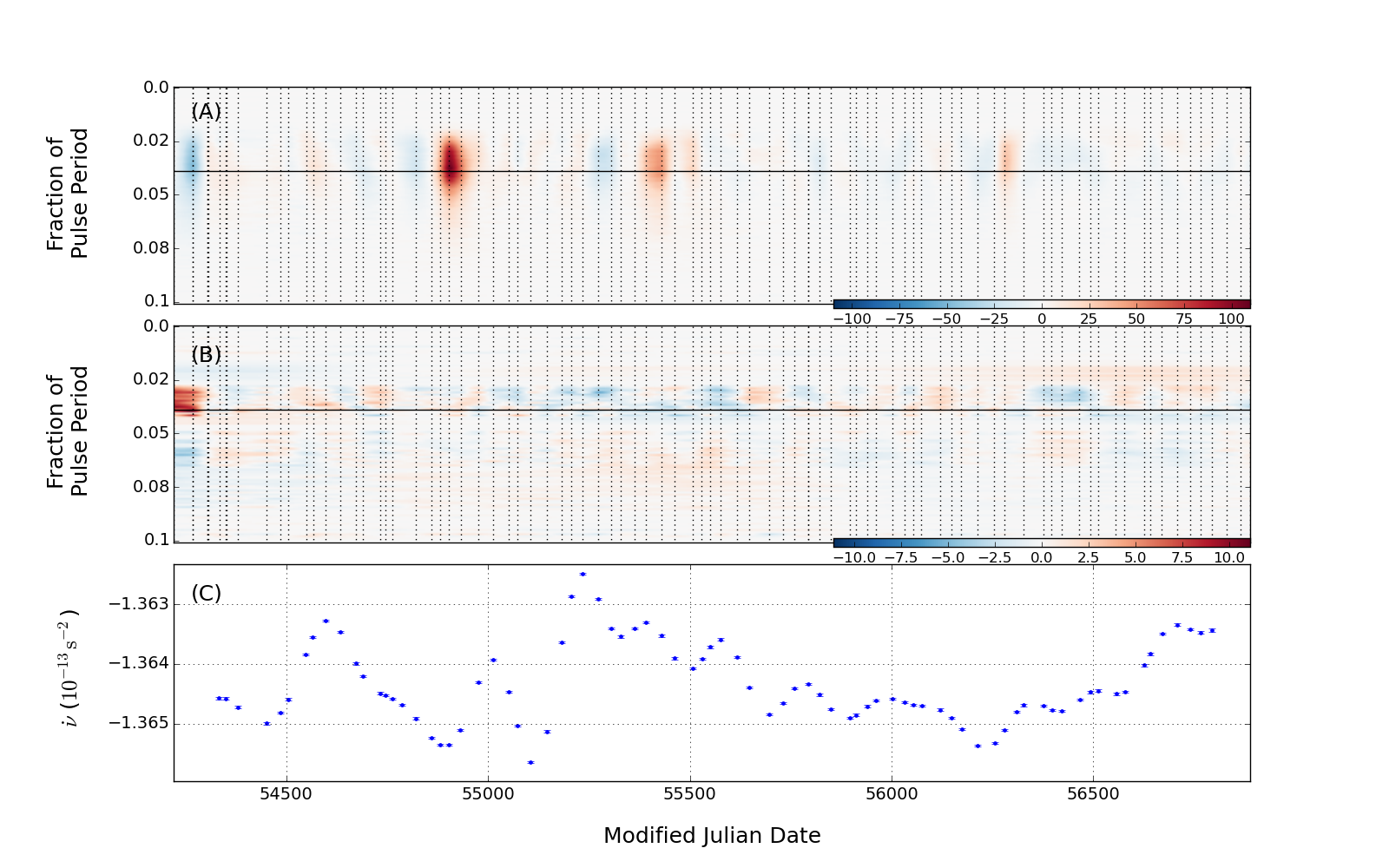
PSR J0738$-$4042 is a bright pulsar with rotational properties typical of the main population of middle-aged, isolated radio pulsars. Despite this, it is known to show a dramatic change in both pulse profile and $\dot{\nu}$, beginning in 2005 and resulting in a new profile component (Karastergiou et al., 2011; Brook et al., 2013). Regular Parkes observations of the pulsar began in March 2008. Figure 3 shows that a prominent change in profile shape occurred in November 2010 ($\sim$ MJD 55525), when the relative size of the transient component (around pulse phase 0.08) increased significantly, and has shown a trend of gradual recession ever since.
Figure 3 shows a pattern of systematic changes that last hundreds of days. In addition, different regions of the profile appear to vary in a correlated or anti-correlated manner. Comparing Panels A and B, shows this to be a good example of a pulsar that exhibits a combination of profile shape changes (Panel B) and total flux density changes (Panel A). Panel C reveals high S/N variability in the estimated $\dot{\nu}$ with what appears to be the periodic signature of a residual error in the position of the pulsar. The value of $\dot{\nu}$ does not display any unusual behaviour around MJD 55525 when the primary change in pulse profile shape occurs.
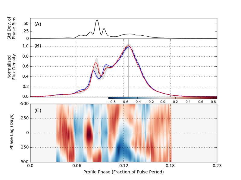
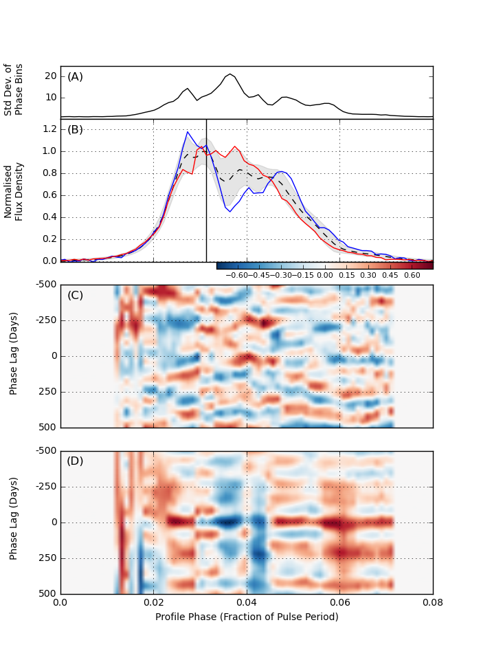
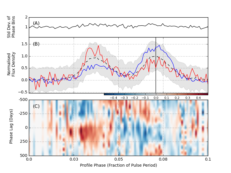
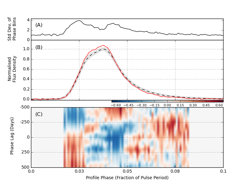
Panel A of Figure 4 highlights the regions of the profile that are most variable. Examples of two significantly different profiles are shown in red and blue in Panel B. Panel C shows a complicated relationship between $\dot{\nu}$ and the profile changes, with highest correlation seen at a pulse phase of $\sim$ 0.075, and a lag of around zero. The previously noted correlation and anti-correlation between regions of the profile can also be seen in Panel C, in the alternating vertical patches.
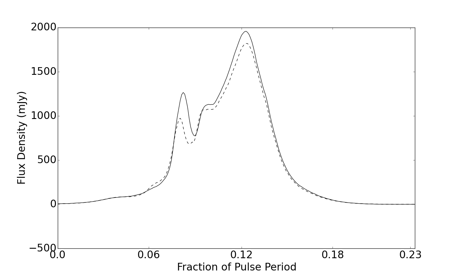
To illustrate the connection between different regions of the profile, in Figure 5 we show the average profile of all the epochs where the transient component is bright and compare it to the average of all remaining epochs. We see that the main component is also brighter when the transient component is bright, and note a small suppression at the leading edge.

Figure 3: Pulse profile and spindown variability for PSR J0738$-$4042. Panel A: Map showing the difference between the flux calibrated observations and the median profile across the dataset. The units are the median of the standard deviation of all off-peak regions of the dataset. The solid horizontal line highlights the profile peak, and the vertical dashed lines show the dates of the included observations. Panel B: As Panel A, but the observations are first normalised by the total flux density of the on-pulse region(s). Panel C: Value of $\dot{\nu}$ on observation dates.

Figure 4: Pulse profile variability and correlation map for PSR J0738$-$4042. Panel A: The standard deviation of the data in each profile phase bin, in units of the mean standard deviation of the off-pulse phase bins. We define an off-pulse phase bin to be one in which the median pulse profile of a dataset is less than 1/30 of its peak. Panel B: Black dashed line traces the median of normalised pulse profiles across all included observations. The blue and red profiles are examples that show the extent of shape changes. The blue profile was observed on MJD 54548, red on MJD 55616. The shaded area denotes 2$\sigma$ above and below the median profile. The solid vertical line marks the peak of the profile. Panel C: SRCC for $\dot{\nu}$ and pulse profile variability as a function of the pulse phase and lag between the two timeseries. A negative lag means that $\dot{\nu}$ is lagging the flux density variability.

Figure 5: Links between the profile shape and the flux density of PSR J0738$-$4042. The solid line traces the median of pulse profiles that were observed between MJD 55525 and MJD 56492, i.e. the epochs over which the transient leading edge component is at its most prominent relative to the profile peak. The dashed line traces the median of the pulse profiles that fall outside this epoch. The solid line shows that when the leading edge component is relatively prominent, the absolute flux density of the profile peak is higher.

4.1.2 PSR J0742$-$2822 (B0740$-$28)

PSR J0742$-$2822 is known to display profile changes that correlate with $\dot{\nu}$ variations (Keith et al., 2013) and exhibits the most rapid changes of the six state-switching pulsars analysed in Lyne et al. (2010).
Panel A of Figure 6 shows the flux density across the whole pulse profile to vary. The individual observations show that the flux density varies by $\sim$ 50% of its median value. The rapid changes in profile shape can be seen in Panel B of Figure 6. This is most pronounced between MJD 55000 and MJD 55500, where the changes in pulse profile can be seen, by eye, to correlate with the $\dot{\nu}$ changes in Panel C of Figure 6. The $\dot{\nu}$ timeseries is very similar to the timeseries published by Keith et al. (2013), using largely the same dataset. As described previously, it is calculated without enforcing a particular window and the error bars are computed using all data that contribute to each point.
Keith et al. summarise the profile changes by introducing a shape parameter. They show that the shape parameter correlates particularly well with $\dot{\nu}$ after a glitch (included in the timing model) occurs at MJD 55022. Because of this, the disorganized pre-glitch correlation map becomes organized post-glitch, where high correlation is observed at zero lag. On closer inspection of Panel C of Figure 7, $\dot{\nu}$ appears to be anti-correlated with the two profile peaks, and correlated with the central trough. In contrast, in Panel D, $\dot{\nu}$ appears to be correlated with the peaks, and anti-correlated with the trough. It follows, and can be seen, that certain phases of the pulse profile are correlated and anti-correlated with others. This phenomenon can also be seen clearly in PSR J0738$-$4042, PSR J1830$-$1059 and PSR J1602$-$5100.
Panel A of Figure 7 shows that the variability across the profile does not follow the profile shape; the maximum variability is near the centre of the profile as show in the examples of Panel B.

Figure 6: Pulse profile and spindown variability for PSR J0742$-$2822. As Figure 3 otherwise.

Figure 7: Pulse profile variability and correlation map for PSR J0742$-$2822. In Panel B, the blue profile was observed on MJD 56642, red on MJD 55445. Panel C shows a correlation map composed of data preceding a glitch on MJD 55022. Panel D is composed only of data after the glitch. Otherwise as Figure 4.

4.1.3 PSR J1830$-$1059 (B1828$-$11)

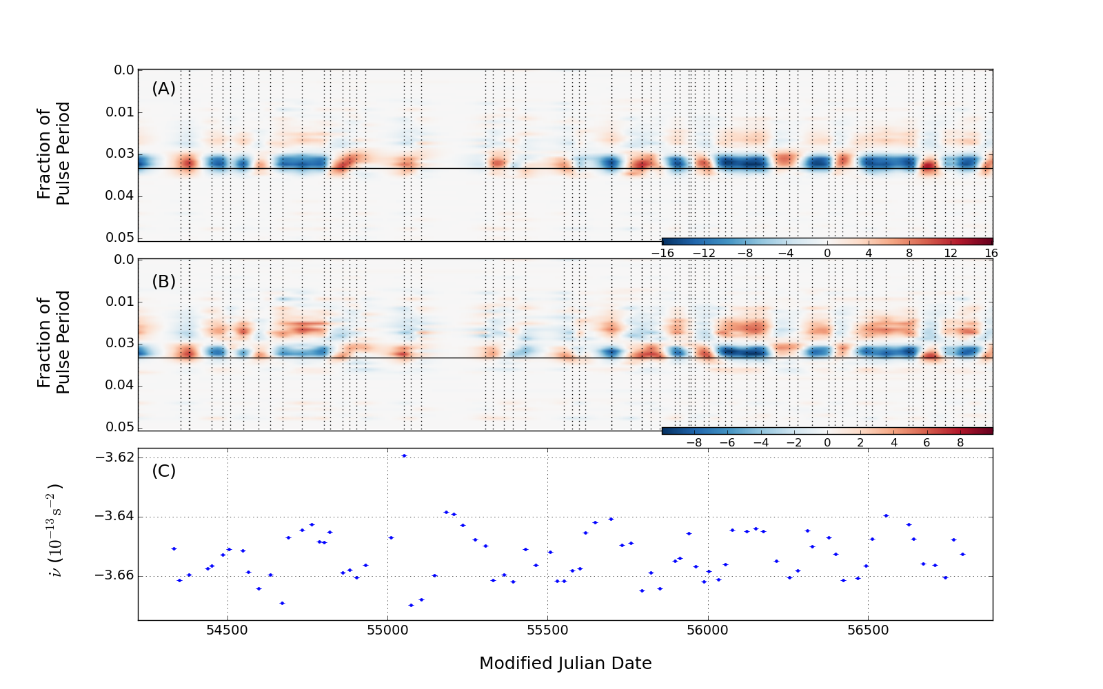
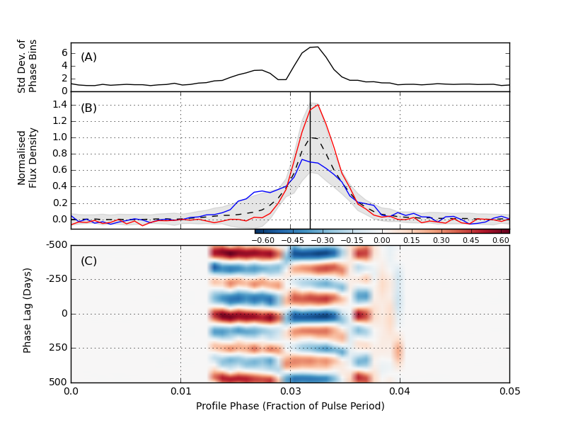
Long-term variability in both the pulse profile shape and spindown rate are well established in PSR J1830$-$1059, along with correlation between the two (Lyne et al., 2010). The variability has been attributed to free precession (Stairs et al., 2000; Jones, 2012) or the effects of an orbiting quark planet (Liu et al., 2007). Quasi-periodic profile changes can be seen clearly in Panels A and B of Figure 8. By eye, these both seem to correlate with $\dot{\nu}$ in Panel C.
The two example profiles in Panel B of Figure 9 illustrate the differences in profile shape, where power from the leading edge migrates to the pulse peak, and vice versa. Panel A shows that the region just before pulse phase 0.03 remains relatively constant.
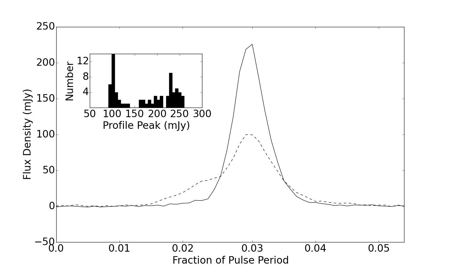
Figure 10 demonstrates that the two profile states have different flux density levels; one has a peak flux density that is more than a factor of two greater than that of the other. The more intense state appears to have a simple profile composed of only one component, whereas the dimmer state has a leading edge component. The mean flux density of the on-pulse region of the two states is not equal; the narrow state has a mean flux density around 1.4 times larger than the wide state.
As a result of the relationship between flux density and profile shape, we see in Figure 8 that the variations in the Panel A also seem to be correlated with those in Panels B and C. This suggests that the observed changes in flux density for PSR J1830$-$1059 are the result of intrinsic processes, rather than propagation effects.
Panel C of Figure 9 shows the correlation between $\dot{\nu}$ and profile shape at each pulse phase, as a function of the lag between the two timeseries. As the pulse profile shape is known to vary in synchronisation with $\dot{\nu}$, we see the strongest correlation occurring around zero lag. We also see that the timseries are correlated when $\dot{\nu}$ has a $\pm$ 500 day lag. This is due to the fact that $\dot{\nu}$ has a cycle of around 500 days, as seen in Panel C of Figure 8.
It is worth noting that the $\dot{\nu}$ variability shows the same pattern of major and minor peaks, as published in Lyne et al. (2010).

Figure 8: Pulse profile and spindown variability for PSR J1830$-$1059. As Figure 3 otherwise.

Figure 9: Pulse profile variability and correlation map for PSR J1830$-$1059. In Panel B, the blue profile was observed on MJD 54548, red on MJD 54381. Otherwise as Figure 4.

Figure 10: Links between the profile shape and flux density of PSR J1830$-$1059. The solid line traces the median of pulse profile that have a peak flux density greater than 150 mJy. The dashed line traces the median of pulse profiles that have a peak flux density lower than 150 mJy. The profiles with the highest flux density are also seen to be the most narrow. The inset shows the flux density level of the profile peaks to be bimodal, reflecting the two states.

4.2 New Variable Pulsars

4.2.1 PSR J0908$-$4913 (B0906$-$49)

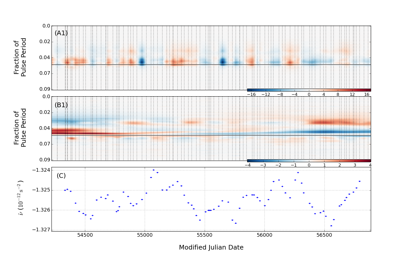
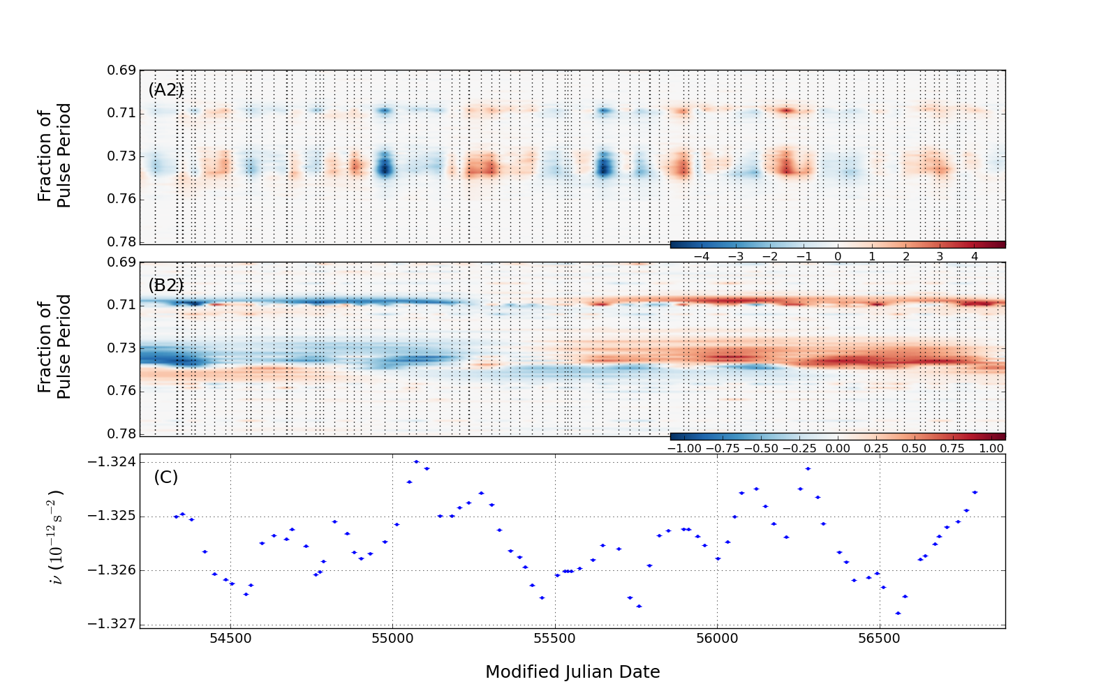
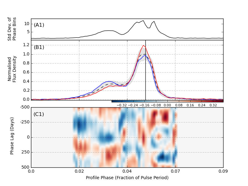
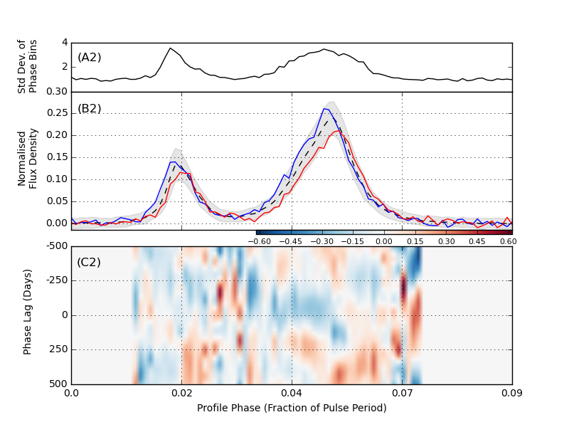
The profile of PSR J0908$-$4913 consists of a main pulse (MP) and an interpulse (IP), and has been show by Kramer & Johnston (2008) to be an orthogonal rotator. Profile-wide flux density variations can be seen in both the MP and IP (Panels A1 and A2 of Figure 11 respectively); the emission received from PSR J0908$-$4913 varies quasi-periodically across the dataset. The flux calibrated profiles vary by up to $\sim$ 50% from the median, which has a peak of around 1000 mJy. The changes in the shape of the pulse profile (Panels B1 and B2 of Figure 11), however, are slight and gradual across the dataset; both IP components and a precursor to the MP steadily grow with respect to the MP. In Panel C, $\dot{\nu}$ shows quasi-periodicity. We see slow variability with three local minima around 54500, 55500 and 56500, between which, we see around four shorter-term cycles. There is no obvious correlation with the shape changes, as is confirmed by the correlation maps in Figure 12. Given the alignment techniques used, the two example profiles in Panels B1 and B2 of Figure 12 show what appears to be a shift in phase in the IP, which is not seen in the MP.

Figure 11: Pulse profile and spindown variability for the MP and IP of PSR J0908$-$4913. Panels A1 and B1 relate to the MP, while Panels A2 and B2 relate to the and IP. As Figure 3 otherwise.

Figure 12: Pulse profile variability and correlation map for the MP and IP of PSR J0908$-$4913. Panels A1, B1 and C1 relate to the MP, while Panels A2, B2 and C2 relate to the IP. In Panel B1 and B2, the blue profile was observed on MJD 56670, red on MJD 54350. Otherwise as Figure 4.

4.2.2 PSR J0940$-$5428

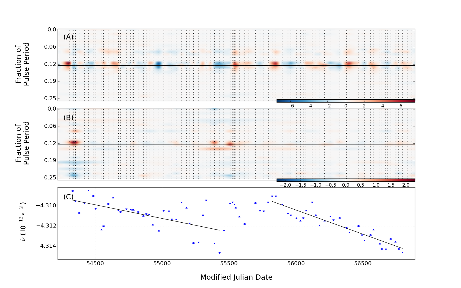
PSR J0940$-$5428 is a faint pulsar; the peak of the median profile is $\sim$ 12 mJy. The pulsar shows only low significance variations in flux density and profile shape (Panels A and B of Figure 13 respectively). We feature PSR J0940$-$5428, however, as an example of $\dot{\nu}$ changes in the absence of significant pulse profile variability. Panel C of Figure 13, shows systematic changes of $\dot{\nu}$ on a time-scale of $\sim$ 200 days, and also two longer-term trends, the gradients of which are marked by solid lines. A steady $\dot{\nu}$ gradient is indicative of a constant $\ddot{\nu}$ term that is absent in the timing model. From left to right, the two $\ddot{\nu}$ terms are $-2.73\times 10^{-18}$ s^-2day^-1 and $-4.80\times 10^{-18}$ s^-2day^-1.
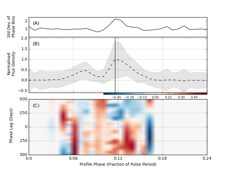
The lack of pulse profile variability is reflected by Panel A and Panel B of Figure 14, in which the deviations of the on-pulse phase bins are comparable to the off-pulse deviations across the profile. As expected, the correlation plot in Panel C of Figure 14 does not show any significant structure.

Figure 13: Pulse profile and spindown variability for PSR J0940$-$5428. The black sold lines in Panel C are best fit to the data points that they span. The left gradient is $-2.73\times 10^{-18}$ s^-2day^-1 and the right gradient is $-4.80\times 10^{-18}$ s^-2day^-1. As Figure 3 otherwise.

Figure 14: Pulse profile variability and correlation map for PSR J0940$-$5428. As Figure 4 except there are no red and blue traces representing pulse profile changes, as they are minimal. This number of phase bins for this pulsar has been reduced to 128.

4.2.3 PSR J1105$-$6107

PSR J1105$-$6107 has a spin period of 63 ms and characteristic age of only 63 kyr. The pulsar has a possible association with a nearby supernova remnant (Kaspi et al., 1997). Both Panel A and Panel B of Figure 15 highlight systematic profile variations. One significant shape change (in the relative size of the two profile components) occurs over several observations, beginning $\sim$ MJD 56500. This change coincides with an increase in $\dot{\nu}$, seen in Panel C. Aside from this, any shape changes are subtle and the profile shape is largely stable across the dataset. This is demonstrated in Panel A of Figure 16; the level of on- and off-pulse profile deviation is approximately the same.
The nature and degree of the profile changes is shown in Panel B of Figure 16. Panel C shows that the highest SRCCs between $\dot{\nu}$ and flux density variability occur around zero lag in the leftmost of the two components.

Figure 15: Pulse profile and spindown variability for PSR J1105$-$6107. As Figure 3 otherwise.

Figure 16: Pulse profile variability and correlation map for PSR J1105$-$6107. In Panel B, the blue profile was observed on MJD 56640, red on MJD 55304. Otherwise as Figure 4.

4.2.4 PSR J1359$-$6038 (B1356$-$60)

The flux density of this pulsar systematically varies by $\sim$ 10% around the median. Panels A and B of Figure 18 indicate that there is some profile variability throughout the dataset, but the most significant shape changes by far occur on three observation days: MJD 56512, 56513 and 56531 (Panel B of Figure 17). The normalised pulse profiles of these observations are substantially wider and shorter than the median profile. Panel C shows that this change in pulse shape approximately coincides with a drop in spindown rate.
Panel A of Figure 18 demonstrates that most variability is occurring at the peak and in the wings of the pulse profile. Panel B shows examples of extreme profile shapes; the red profile reflects the shape of the three anomalous observations discussed above. This profile is mostly outside the grey 2$\sigma$ bands of the median profile, confirming that these short-term profile shape changes exceed the typical level of profile variability across the dataset. In Panel C of Figure 18, the highest level of correlation is seen when the $\dot{\nu}$ variability lags the flux density variability by 250 days (a phase lag of -250 days).

Figure 17: Pulse profile and spindown variability for PSR J1359$-$6038. As Figure 3 otherwise.

Figure 18: Pulse profile variability and correlation map for PSR J1359$-$6038. In Panel B, the blue profile was observed on MJD 54268, red on MJD 56512. Otherwise as Figure 4.

4.2.5 PSR J1600$-$5044 (B1557$-$50)

Observations of this pulsars over a 13 year dataset from Hartebeesthoek Radio Astronomy Observatory showed evidence of cyclic variations in both the dispersion measure and $\dot{\nu}$ of PSR J1600$-$5044 (Chukwude, 2002). The two appear anti-correlated, and are attributed to free precession of the pulsar.
In the Parkes dataset, flux calibrated observations of PSR J1600$-$5044 show significant variability; the peak of the median profile is $\sim$ 800 mJy, which increases systematically to $\sim$ 1500 mJy (MJD 54902) before dropping back to the level of the median value. The process occurs over $\sim$ 120 days and can be seen in Panel A of Figure 19). These flux density variations are expected to be largely due to refractive scintillation, and are eliminated by the normalisation process. Panel B shows that no significant variability is seen in pulse profile shape, with the exception of the first two observations of the dataset. Slow $\dot{\nu}$ variability is seen in Panel C, between which, shorter-term cycles are observed.
In Figure 20, Panel A shows that the most variability occurs at the leading and trailing edges of the pulse profile; the median value is shown in Panel B. The red trace in this panel represents the profile shape of the first two observations in the dataset. The narrow nature of the grey 2$\sigma$ bands demonstrates the relative stability of the profile. The correlation plot in Panel C of Figure 20 does not show significant structure. This is expected, due to the lack of profile shape variation in the dataset.

Figure 19: Pulse profile and spindown variability for PSR J1600$-$5044. As Figure 3 otherwise.

Figure 20: Pulse profile variability and correlation map for PSR J1600$-$5044. The red profile was observed on MJD. This profile shape is seen in the only two observations with noticeable deviations from the median. As Figure 4 otherwise

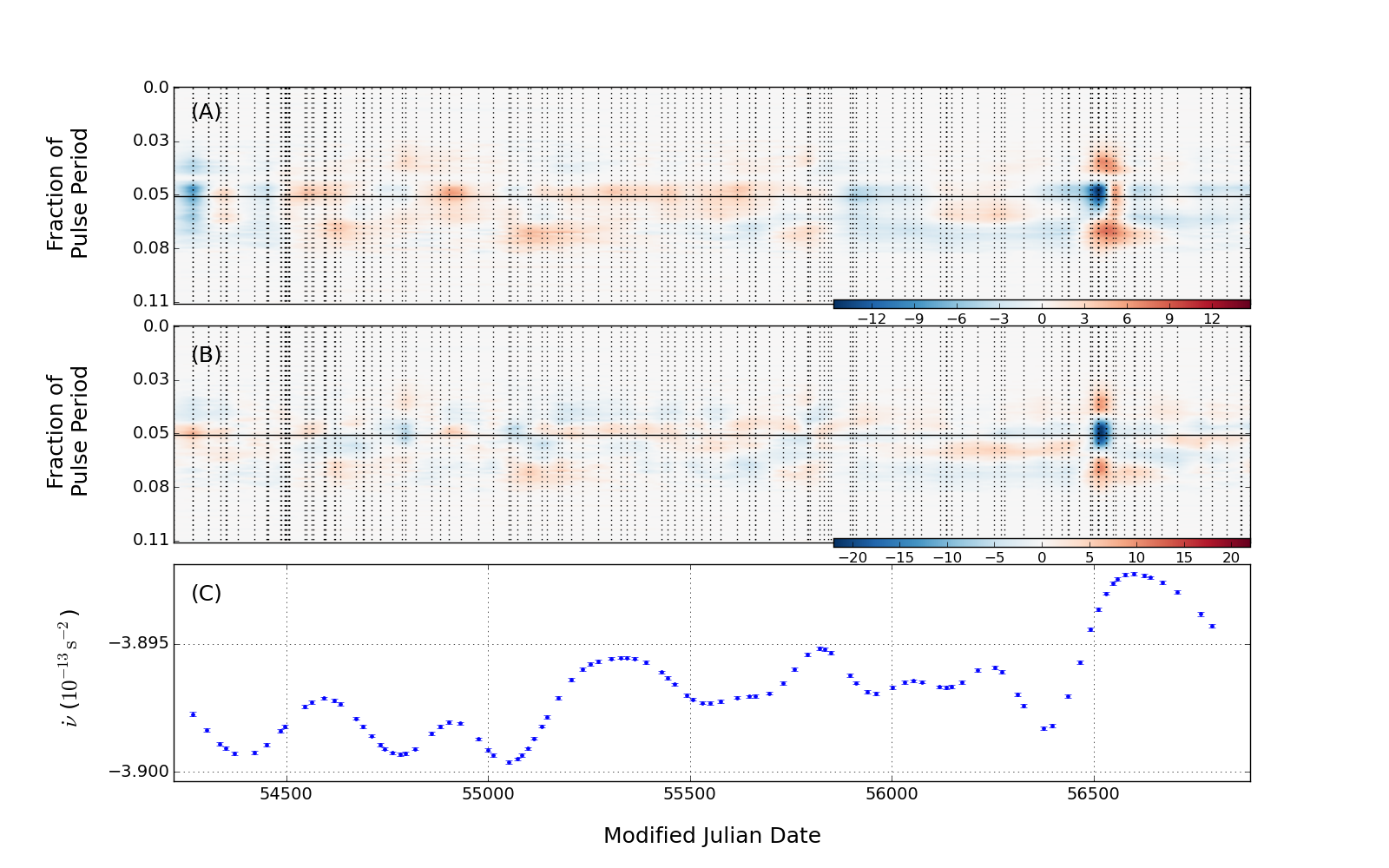
4.2.6 PSR J1602$-$5100 (B1558$-$50)

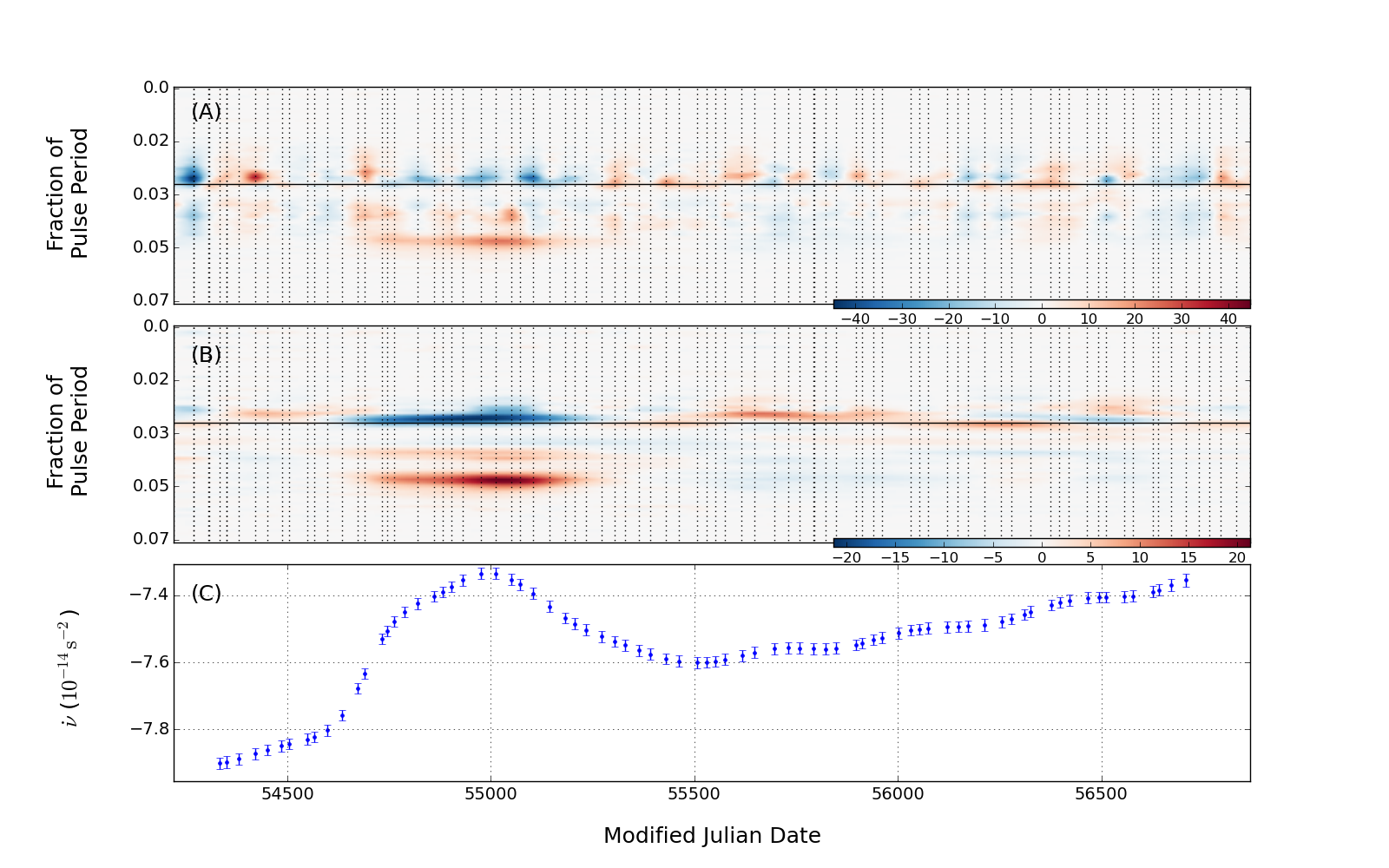
PSR J1602$-$5100 has the smallest spin frequency of the nine pulsars featured in this work, and consequently only PSR J0738$-$4042 has a lower spindown luminosity $\dot{E}$. A dramatic change in the pulse profile can be seen in both Panel A and Panel B of Figure 21, beginning at $\sim$ MJD 54700 and occurring over $\sim$ 600 days. A drop in $\dot{\nu}$ of $\sim$ 5%, which is correlated with the shape change, can be seen in Panel C; both sets of variations appear to begin, peak and end at approximately the same time.
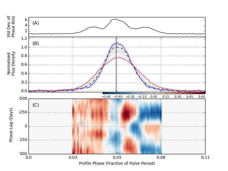
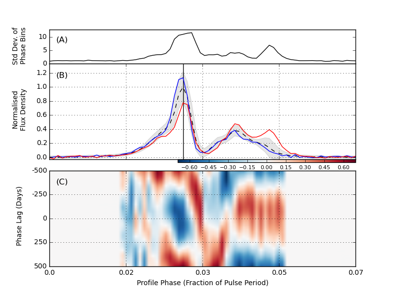
Panel A of Figure 22 shows that the most variability occurs in the profile peak, and in a trailing edge component. The extent of the pulse profile shape variations can be seen in Panel B. In the correlation map (Panel C), SRCC between $\dot{\nu}$ and flux density variability is seen to be strongest around the pulse profile phase at which the transient component appears. The rising baseline of $\dot{\nu}$ (indicative of an unmodelled $\ddot{\nu}$ parameter) was flattened prior to the correlation calculations.
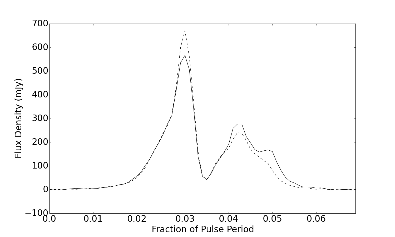
The flux calibrated observations show that the appearance of the new peak at the trailing edge of the smaller profile component coincides with a drop in flux density at the primary profile component (Figure 23).

Figure 21: Pulse profile and spindown variability for PSR  J1602$-$5100. As Figure 3 otherwise.

Figure 22: Pulse profile variability and correlation map for PSR J1602$-$5100. In the middle panel, the blue profile was observed on MJD 54420, red on MJD 55072. Otherwise as Figure 9.

Figure 23: Links between the profile shape and the flux density of PSR J1602$-$5100. The solid line traces the median of pulse profiles that were observed between MJD 54672 and MJD 55304, i.e. the epoch over which the transient component appeared. The dashed line traces the median of the pulse profiles that fall outside this epoch. When the transient trailing edge component is present, the peak flux is seen to fall.

4.3 Other Pulsars in the Dataset

The pulsars described above were chosen because they displayed some type of noteworthy variability. The pulse profile variability maps of all 168 pulsars in our dataset were assessed by eye. A non-detection of variability results from a stable pulse profile, but also from variations that are undetectable due to an insufficient S/N. The extent to which variability can be detected in noisy profiles is discussed in the next section.
Performing the rotational variability analysis revealed that many of the pulsars in our dataset displayed a yearly cycle in $\dot{\nu}$, signifying a positional inaccuracy in the pulsar timing model. Rotational variability may, therefore, remain hidden in those pulsars. We leave it for future work to investigate whether our modelling technique can be used to better determine the position and proper motion, as opposed to techniques involving the removal of timing noise (Coles et al., 2011).
When analysing profile variability, only 9 out of the 168 pulsars show significant profile shape changes. PSR J1302$-$6350 and PSR J1825$-$0935 were not featured in this work but our analysis revealed their known variability (Johnston et al., 1994; Lyne et al., 2010). In order to determine the type of profile variability that can pass undetected by our analysis techniques, we produced a series of simulated pulsar datasets. Artificial pulse profiles were created and spaced approximately 30 days apart, spanning around 5 years in duration. The pulse profile begins as a simple Gaussian function. After around a year of the simulation, a small transient component grows and recedes on the trailing edge of the profile over the course of 3 years of the simulation. Noise with a standard deviation of 0.02 of the main pulse peak was added to all profiles. The effects of refractive scintillation were simulated by scaling each profile by a random factor. 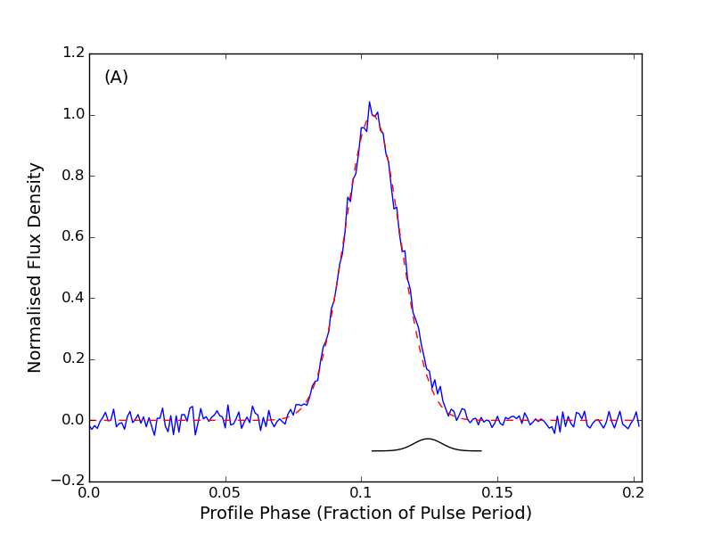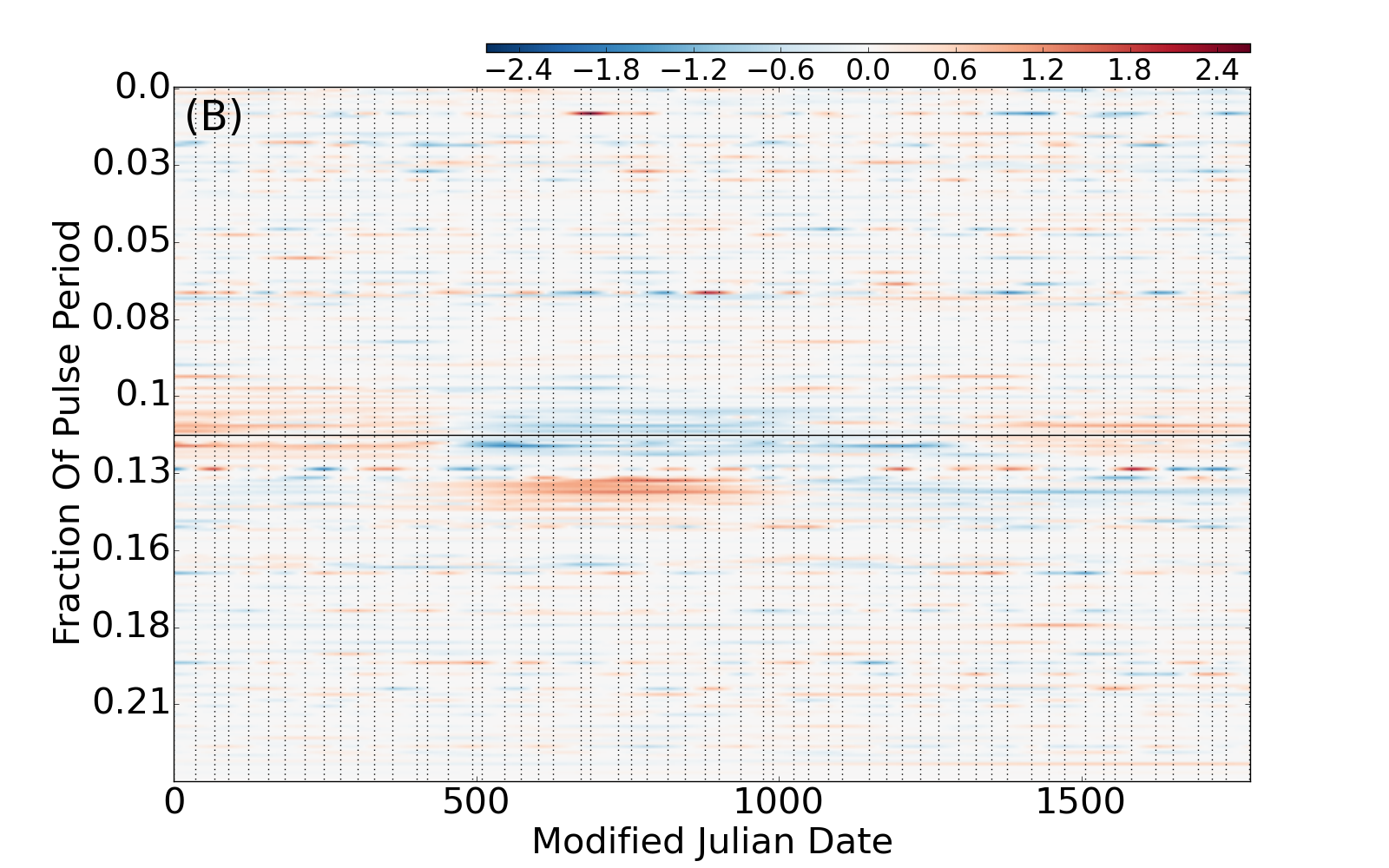The factor is drawn from a distribution around 1.0 with a standard deviation of 0.2. Panel A of Figure 24 shows the almost imperceivable transient component (between phase fraction 1.2 and 1.3) at its maximum. In this case, the peak of the component was chosen to be twice the standard deviation of the noise added to the profiles. Despite the apparently subtle nature of the profile variation, it can be clearly seen in the corresponding variability map (Panel B of Figure 24). This is because GP regression is sensitive to even faint trends that persist over multiple data points.
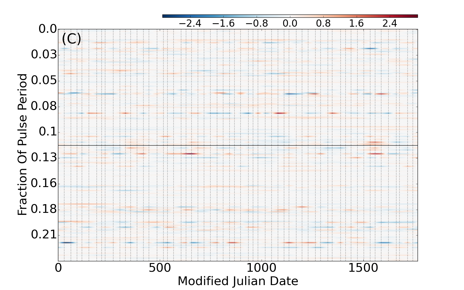
To mimic the case in which the profile variability has a time-scale comparable or shorter than the observing cadence, we shuffled the pulse profiles so that the growth and recession of the transient component was no longer coherent. The resulting variability map shown in Panel C of Figure 24. Although the magnitude of the profile deviation is the same, the variability is not highlighted by the detection technique. When GP regression is employed to model the flux density variability seen in each pulse phase bin, any profile features that occur in single observations only, will have little effect on the model and, therefore, on the emission variability map overall. This is desirable if the single observation has produced a spurious pulse profile due to instrumental failure, but conversely, any genuine profile deviations that occur in single observations may not feature in the final emission variability map.

Figure 24: The variability maps resulting from simulated pulse profiles. Over the $\sim$ 5 year simulation, a transient components grows and recedes over a $\sim$ 2.5 year span, on the trailing edge of the pulse profile. Panel A shows a comparison between the noiseless profile template (red dashed line) and the profile at the height of its deviation with noise included (blue solid line). The transient component is shown (at its most prominent) at the phase at which it appears, as a black solid line. Panels B and C show the difference between the simulated profiles and the profile template. The units are the median of the standard deviation of all off-pulse regions of the simulated profiles. The solid horizontal line highlights the profile peak, and the vertical dashed lines show the date of the simulated observations. Panel B is the variability map that results from this simulated dataset. Panel C shows the variability map that results after the simulated profiles are randomly shuffled in time.

5 Discussion

5.1 New Techniques

We have developed a new technique for measuring $\dot{\nu}$ by employing GP regression to model the second derivative of the timing residuals. The uncertainty of our $\dot{\nu}$ values is small because the GP regression prediction at any point is informed by many neighbouring data points (the extent of which is dependent on the covariance parameters). As described in Section 3.2, our techniques provide fully Bayesian error estimation, which is not the case when timing residuals are modelled using a maximum likelihood estimator. Additionally, the method is analytical, in contrast to previous techniques, in which $\dot{\nu}$ is numerically calculated from the information within the span of a small window.
When fitting a non-parametric function to the timing residuals, all but two of the nine pulsars featured in this paper were best fit by a covariance function that contained two squared exponential kernels plus a noise model. Table 2 shows the optimised covariance parameters when fitting the timing residuals with one and with two kernels in the covariance function. Where the data is best fit by two kernels, this suggests that at least two physical processes are responsible for the timing noise that we observe.
Using the above technique to measure $\dot{\nu}$, along with our method to map pulse profile shape changes, we have been able to reproduce the quasi-periodic variability already observed in PSR J0742$-$2422 (Lyne et al., 2010; Keith et al., 2013) and PSR J1830$-$1059 (Lyne et al., 2010).
A very useful property of a GP, is that it can combine derivative and integral observations. If, in the future, we are able to successfully use pulse profile variability as a proxy to calculate $\dot{\nu}$ values, these data can be easily combined with timing residuals in further GP regression.

5.2 PSR J1602$-$5100

The above techniques have also uncovered a striking new example of correlated $\dot{\nu}$ and profile shape variability in PSR J1602$-$5100. This pulsar exhibits a dramatic change in profile shape over $\sim$ 600 days, with a simultaneous reduction in $\dot{\nu}$. Such sudden and dramatic changes have previously been attributed to exterior material entering the pulsar magnetosphere (Cordes & Shannon, 2008; Shannon et al., 2013; Brook et al., 2013). The reconfiguration in current within the magnetosphere, induced by the introduction of external material, would simultaneously affect the braking torque and hence $\dot{\nu}$. The value of $\dot{\nu}$ of PSR J1602$-$5100 is observed to decrease with the appearance of a new profile component. This is comparable to the 2005 event seen in PSR J0738$-$4042, hypothesised to be caused by an asteroid encounter (Brook et al., 2013). The changes observed in PSR J0738$-$4042 have persisted, whereas PSR J1602$-$5100 returned to its previous state after $\sim$ 600 days. The change in $\dot{\nu}$ over this period can be approximated as a step-function, and interpreted as a reduction in the total outflowing plasma above the polar caps. The magnitude of the current change can be inferred from the change in $\dot{\nu}$ following Kramer et al. (2006). The difference between the pre- and post-step $\dot{\nu}$ values corresponds to a reduction in the charge density $\rho$ of $\sim 9\times 10^{-9}$ C cm^-3, where $\rho=3I\Delta\dot{\nu}/R_{pc}^{4}B_{0}$, the moment of inertia $I$ is taken to be 10⁴⁵ g cm², the magnetic field $B_{0}=3.2\times 10^{19}\sqrt{-\dot{\nu}/\nu^{3}}$ G, polar cap radius $R_{pc}=\sqrt{2\pi R^{3}\nu/c}$ and where the neutron star radius $R$ is taken to be $10^{6}$ cm. We can relate the difference in charge density associated with the two $\dot{\nu}$ states to mass supplied to the pulsar, by multiplying it by the speed of light, the polar cap area and the duration of the new spindown state. Over 600 days (the duration of the dramatic profile and $\dot{\nu}$ changes), this amounts to $\sim 10^{14}$ g, which lies within the range of known solar system asteroid masses, and is consistent with the mass range of asteroids around neutron stars proposed by Cordes & Shannon (2008).

5.3 Correlated Variability

The present interpretation of the correlated long-term variations observed in emission and rotation, involves charged particle currents in the pulsar magnetosphere (Kramer et al., 2006); distinct pulsar states can be explained by differing levels of magnetospheric plasma. Changing plasma levels are expected to modify both the material outflow along open field lines at the polar cap, and the subsequent emission produced. Plasma variations would also vary the braking torque on the pulsar, and we would expect to see a change in $\dot{\nu}$ accompanying any significant change in emission. The correlated variability that has been previously observed in pulse profiles and rotation are, therefore, evidence of intrinsic processes.
In this paper, we have demonstrated that pulse profile shape can be shown to correlate with $\dot{\nu}$, although the relationship does not appear to be simple. Of the nine pulsars analysed in this paper, seven show significant changes in pulse profile shape to various degrees and on various time-scales. Of those, five also show some degree of $\dot{\nu}$ variation that could be considered correlated. It is particularly interesting that no change in $\dot{\nu}$ is seen to accompany the dramatic profile shape change seen in PSR J0738$-$4042.
When interpreting these results, we must consider the possibility that the relationship beween $\dot{\nu}$ and pulse profile variability is more complex than anticipated and/or that the relationship is simple, but that we are unable to accurately record the variability involved. When analysing the rotational variations, for example, we have made the hypothesis that timing noise is due to changes in the braking torque on the pulsar, observable as changes in $\dot{\nu}$. Other possible sources of timing noise are, inadequate calibration of the raw observations (e.g. van Straten, 2006), and failure to correct for variations in the interstellar dispersion (e.g. You et al., 2007). With regard to the pulse profile variability analysis, the simulation described in Section 4.3 demonstrates that trends that persist over multiple observations can be detected by the techniques described in this work, providing they have a magnitude above $\sim$ two times the level of the observation noise. Therefore, profile faint variability that also has a short time-scale will often go undetected. Additionally, when testing the correlation between the variability of flux density in individual (or small groups of) pulse phase bins and the spindown rate, we acknowledge that the latter is measured much more accurately than the former. Longer observation times would, in general, produce more stable pulse profiles and allow extraordinary deviations to be more easily identified. The standard deviation of the mean profile is proportional to 1/$\sqrt{n}$, where $n$ is the number of pulses it includes. 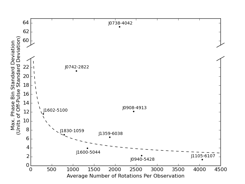As each pulsar has a different rotational period, and has observations of varying length, the degree of their profile stability is also expected to be different. Figure 25 plots the average number of rotations in an observation against the maximum amount of deviation in the pulse profile. It is interesting to note that most of the pulsars featured in this paper follow the expected trend, with the stark exception being PSR J0738$-$4042; sections of the pulse profile clearly remain unstable since the dramatic changes undergone in 2005. PSR J0742$-$2822 and PSR J0908$-$4913 also show substantially more deviation than that expected from their average observation length.

Figure 25: The maximum amount of deviation of a pulsar’s profile as a function of the average number of rotations per observation. The dashed line shows the $y=1/\sqrt{x}$ function that best fits all data points with the exception of PSR J0738$-$4042, PSR 0742$-$2822 and PSR J0908$-$4913.

5.4 The Relationship Between Shape and Mean Flux Density

We have shown that changes in the shape of the pulse profile can be accompanied by changes in its mean flux density. This is seen most clearly in PSR J1830$-$1059, in which the narrow emission state has a mean flux density around 1.4 times larger than the wide state. In other words, the flux density of the leading edge component and of the peak are in anti-correlation. Such anti-correlation (and correlation) is also seen in other pulsars, most notably PSR J0738$-$4042 and PSR J1602$-$5100.
For PSR J1830$-$1059, it is possible to predict the spindown rate from the radio flux density received from the pulsar. In this respect, parallels can be drawn between the behaviour of PSR J1830$-$1059 and that of the intermittent pulsars; both have two states in which higher emission is coupled to more rapid spindown.
The relationship between pulse profile shape and mean flux density cannot be easily investigated in most pulsars, because large variations in pulse profile flux density, due to refractive scintillation, are ubiquitous; the pulse profile varies as a whole, and its shape is maintained. For some pulsars, these flux density variations are coherent over multiple observations, i.e., on a time-scale of hundreds of days. As these variations are thought to be primarily due to effects of propagation, we expect, and find, that pulse profile flux density and $\dot{\nu}$ are not well correlated in general. It is for this reason that the correlation maps produced in this work show the relationship between the normalised pulse profiles and $\dot{\nu}$. It should be noted that the nature of the normalisation process itself can result in some apparent anti-correlation between different phases of the pulse profile.
When considering the changing shape of a pulse profile, it is noteworthy that throughout the normalised flux density plots in this paper, we see varying levels of deviation across the pulse profile. For example, the standard deviation in one leading edge component of PSR J0738$-$4042 is $\sim$ 63 times larger than the mean standard deviation seen across the off-pulse phase bins (Panels A and B of Figure 4). This is in contrast to other sections of the profile that show much less deviation. Further investigation of single pulses would elucidate the differing levels of deviation across a pulse profile. This fact also offers the opportunity to improve pulsar timing by preferentially employing the most stable sections of the pulse profile when performing template matching.

6 Conclusions

We have analysed 168 pulsar datasets, each spanning up to eight years in length, and presented results from nine pulsars. We have employed GP regression as part of new analysis techniques in order to model pulse profile variability. Simulations have shown that this is most easily detected if the profile deviations occur over multiple observations and have a magnitude at least twice the level of the observational noise.
GP regression was also used to infer $\dot{\nu}$ under the assumption that all timing noise is the result of unmodelled changes in $\dot{\nu}$. Our variability detection techniques have accurately reproduced known pulsar variability, and also discovered some clear new examples. The most notable new variability was found in PSR J1602$-$5100; dramatic pulse profile changes along with a $\sim$ 5% rise and fall in $\dot{\nu}$ occur simultaneously over a $\sim$ 600 day span.
The correlation between $\dot{\nu}$ and changes in pulse profile shape is clear in some pulsars, but not in others. We must consider that one or more of the following is true: (i) The intrinsic relationship between $\dot{\nu}$ and pulse profile variability is possibly more complex than has been postulated previously. (ii) Our ability to detect pulse profile variability is often insufficient to show the underlying correlation with $\dot{\nu}$. (iii) Our hypothesis that unmodelled changes in $\dot{\nu}$ are primarily responsible for timing noise, may be invalid. Problems regarding the detection of pulse profile variability will be mitigated by more sensitive instruments and longer integration times.
Finally, we have observed a strong relationship between the shape changes of PSR J1830$-$1059 and its mean flux density, both of which are correlated with $\dot{\nu}$. One pulse profile shape has a mean flux density around 1.4 times that of the other, meaning that the monitoring of either the profile shape or the mean flux density would permit the removal of most of the timing noise in this pulsar.

References

- Backer (1970a) Backer D. C., 1970a, Nature, 228, 42
- Backer (1970b) Backer D. C., 1970b, Nature, 228, 1297
- Brook et al. (2013) Brook P. R., Karastergiou A., Buchner S. et al., 2014, ApJ, 780, L31
- Camilo et al. (2007) Camilo, F. Cognard I., Ransom S. M. et al., 2007, ApJ, 663, 497
- Camilo et al. (2012) Camilo F., Ransom S. M., Chatterjee S., Johnston S., Demorest P., 2012, ApJ, 746, 53
- Chukwude (2002) Chukwude A. E., 1997, African Skies, 7, 41
- Coles et al. (2011) Coles W., Hobbs G., Champion D. J., Manchester R. N., Verbiest J. P. W., 2011, MNRAS, 418, 561
- Cordes & Shannon (2008) Cordes J. M., Shannon R. M., 2008, ApJ, 682, 1152
- Deng et al. (2012) Deng X. P., Coles W., Hobbs G. et al., 2012, MNRAS, 424, 244
- Gaensler et al. (1998) Gaensler B. M., Stappers B. W., Frail D. A., Johnston S., 1998, ApJ, 499, L69
- Hobbs et al. (2006) Hobbs G. B., Edwards R. T., Manchester R. N., 2006, MNRAS, 369, 655
- Holsclaw et al. (2013) Holsclaw T. et al., 2013, Technometrics, 55:1, 57-67, DOI: 10.1080/00401706.2012.723918
- Johnston et al. (1994) Johnston S., Manchester R. N., Lyne A. G. et al., 1994, MNRAS, 268, 430
- Jones (2012) Jones D. I., 2012, MNRAS, 420, 2325
- Karastergiou et al. (2011) Karastergiou A., Roberts S. J., Johnston S. et al., 2011, MNRAS, 415, 251
- Kaspi et al. (1997) Kaspi V. M., Bailes M., Manchester R. N. et al., 1998, ApJ, 499, L69
- Keith et al. (2013) Keith M. J., Shannon R. M., Johnston S., 2013, MNRAS, 423, 3080
- Kramer et al. (2006) Kramer M., Lyne A. G., O’Brien J. T., Jordan C. A., Lorimer D. R., 2006, Science, 312, 549
- Kramer & Johnston (2008) Kramer M., Johnston S., 2008, MNRAS, 390, 87
- Liu et al. (2007) Liu K., Yue Y. L., Xu R. X., 2007, MNRAS, 381, L1
- Lorimer et al. (2012) Lorimer D. R., Lyne A. G., McLaughlin M. A. et al., 2012 ApJ, 758, 141
- Lyne et al. (2010) Lyne A., Hobbs G., Kramer M., Stairs I., Stappers B., 2010, Science, 329, 408
- Rasmussen & Williams (2006) Rasmussen C. E., Williams C. K. I., 2006, Gaussian Processes for Machine Learning, The MIT Press
- Roberts et al. (2012) Roberts S., Osborne M., Ebden M. et al., 2012, Phil. Trans. R. Soc. A, 371
- Shannon et al. (2013) Shannon R. M., Cordes J. M., Metcalfe T. S. et al., 2013, ApJ, 766, 5
- Stairs et al. (2000) Stairs I. H., Lyne A. G., Shemar S. L., 2000, Nature, 406, 484
- van Straten (2004) van Straten W., 2004, ApJS152, 129
- van Straten (2006) van Straten W., 2006, ApJ642, 1004
- Wang et al. (2007) Wang N., Manchester R. N., Johnston S., 2007, MNRAS, 377, 1383
- Weltevrede et al. (2010) Weltevrede P., Johnston S., Manchester R. N. et al., 2010, Proc. Astr. Soc. Aust., 27, 64
- Weltevrede et al. (2011) Weltevrede P., Johnston S., Espinoza C. M., 2011, MNRAS, 411, 1917
- Woods & Thompson (2006) Woods P. M., Thompson C., 2006, in Compact Stellar X-Ray Sources, ed. Lewin W. H. G., van der Klis M., (Cambridge: Cambridge Univ. Press), 547
- You et al. (2007) You X. P., Hobbs G., Coles W. A. et al., 2007, MNRAS, 378, 493