A fast method to estimate speciation parameters in a model of isolation with an initial period of gene flow
and to test alternative evolutionary scenarios.

Abstract

We consider a model of “isolation with an initial period of migration” (IIM), where an ancestral population instantaneously split into two descendant populations which exchanged migrants symmetrically at a constant rate for a period of time but which are now completely isolated from each other. A method of Maximum Likelihood estimation of the parameters of the model is implemented, for data consisting of the number of nucleotide differences between two DNA sequences at each of a large number of independent loci, using the explicit analytical expressions for the likelihood obtained in Wilkinson-Herbots (2012). The method is demonstrated on a large set of DNA sequence data from two species of Drosophila, as well as on simulated data. The method is extremely fast, returning parameter estimates in less than 1 minute for a data set consisting of the numbers of differences between pairs of sequences from 10,000s of loci, or in a small fraction of a second if all loci are trimmed to the same estimated mutation rate. It is also illustrated how the maximized likelihood can be used to quickly distinguish between competing models describing alternative evolutionary scenarios, either by comparing AIC scores or by means of likelihood ratio tests. The present implementation is for a simple version of the model, but various extensions are possible and are briefly discussed.

Introduction

In recent years, molecular genetic data have been used extensively to learn about the evolutionary processes that gave rise to the observed genetic variation. One important example is the use of genetic data to try to infer whether or not gene flow occurred between closely related species during or after speciation (see for example reviews by Nadachowska 2010, Pinho and Hey 2010, Smadja and Butlin 2011, Bird et al. 2012 and a large number of references in these papers). Such applications typically use computer programs such as MDIV (Nielsen and Wakeley 2001), IM (Hey and Nielsen 2004, Hey 2005), IMa (Hey and Nielsen 2007), MIMAR (Becquet and Przeworski 2007) or IMa2 (Hey 2010), based on the “isolation with migration” (IM) model, which assumes that a panmictic ancestral population instantaneously split into two or more descendant populations some time in the past and that migration occurred between these descendant populations at a constant rate ever since. Whilst such methods have been extensively and successfully applied to study the relationships between different populations within species, the assumption of migration continuing at a constant rate until the present is unrealistic when studying relationships between species. Becquet and Przeworski (2009) and Strasburg and Rieseberg (2010) investigated by means of simulations how robust parameter estimates (migration rates, divergence times and effective population sizes), obtained by methods based on the IM model, are to violations of the IM model assumptions. Becquet and Przeworski (2009) found that parameter estimates obtained with IM and MIMAR are often biased when the assumptions of the IM model are violated, and concluded that these methods are highly sensitive to the assumption of a constant migration rate since the population split. Theoretical results derived by Wilkinson-Herbots (2012) also suggested that estimated levels of gene flow obtained by applying an IM model to species which are now completely isolated cannot simply be interpreted as average levels of gene flow over time. Thus, whilst computer programs based on the IM model can be used to test for departure from a complete isolation model (which assumes that an ancestral population instantaneously split into two or more descendant populations which have been completely isolated ever since), the actual parameter estimates obtained may be difficult to interpret if the IM model is not an accurate description of the history of the populations or species concerned. Furthermore, in some studies the programs IMa or IMa2 have also been used to estimate the times when migration events occurred, and to try to distinguish between scenarios of speciation with gene flow and scenarios of introgression, and it has recently been demonstrated that such inferences about the timing of gene flow (obtained with programs based on the IM model) are not valid (Strasburg and Rieseberg 2011, Sousa et al. 2011). Becquet and Przeworski (2009), Strasburg and Rieseberg (2011) and Sousa et al. (2011) all suggested that more realistic models of population divergence and speciation are needed.

A first step in trying to make the IM model more suitable for the study of speciation is to allow gene flow to occur during a limited period of time, followed by complete isolation of the species, and such models have been studied by Teshima and Tajima (2002), Innan and Watanabe (2006) and Wilkinson-Herbots (2012). In the latter paper, a model of “isolation with an initial period of migration” (IIM) was studied where a panmictic ancestral population gave rise to two or more descendant populations which exchanged migrants symmetrically at a constant rate for a period of time, after which they became completely isolated from each other. Explicit analytical expressions were derived for the probability that two DNA sequences (from the same descendant population or from different descendant populations) differ at $k$ nucleotide sites, assuming the infinite sites model of neutral mutation. It was suggested that these results may be useful for Maximum Likelihood estimation of the parameters of the model, if one pair of DNA sequences is available at each of a large number of independent loci, and that such an ML method should be very fast as it is based on an explicit expression for the likelihood rather than on computation by means of numerical approximations or MCMC simulation. However the proposed ML estimation method had not yet been implemented and its usefulness was still to be demonstrated. In this paper we present an implementation of the ML estimation method for the parameters of the “isolation with an initial period of migration” model proposed in Wilkinson-Herbots (2012), and we illustrate its potential by applying it to a set of DNA sequence data from Drosophila simulans and Drosophila melanogaster previously analysed by Wang and Hey (2010) and Lohse et al. (2011). The parameter estimates and maximized likelihood obtained for the IIM model are also compared to those under an IM model and an isolation model, and it is illustrated that the method makes it possible to distinguish between more and less plausible evolutionary scenarios, by comparing AIC scores or by means of likelihood ratio tests. The implementation was done in R (R Development Core Team 2011). The R code for the MLE method described is included as Supplementary Material and can readily be pasted into an R document. This MLE algorithm is very fast indeed: for the Drosophila data mentioned above (using the number of nucleotide differences between two DNA sequences at each of approximately 30,000 loci), we obtained estimates of the parameters of the IIM model using a desktop PC; the program returned results instantly (i.e. in a small fraction of a second) if all loci had been trimmed to the same estimated mutation rate (as proposed by Lohse et al. 2011), or in approximately 20 seconds if the full sequences (and hence different mutation rates at different loci) were used.

Whereas most earlier methods used large samples from a small number of loci, recent advances in DNA sequencing technology and the advent of whole-genome sequencing have led to an increased interest in methods which (like that described in this paper) can handle data from a small number of individuals at a large number of loci (for example, Takahata 1995; Takahata et al. 1995; Takahata and Satta 1997; Yang 1997, 2002; Innan and Watanabe 2006; Wilkinson-Herbots 2008; Burgess and Yang 2008; Wang and Hey 2010; Yang 2010; Hobolth et al. 2011; Li and Durbin 2011; Lohse et al. 2011; Wilkinson-Herbots 2012; Zhu and Yang 2012; Andersen et al. 2014). This type of data set has two advantages. Firstly, data from even a very large number of individuals at the same locus tend to contain only little information about very old divergence or speciation events because typically the individuals’ ancestral lineages will have coalesced to a very small number of ancestral lineages by the time the event of interest is reached, and in such contexts a data set consisting of a small number of DNA sequences at each of a large number of independent loci may be more informative (Maddison and Knowles 2006; Wang and Hey 2010; Lohse et al. 2010, 2011). Secondly, considering small numbers of sequences at large numbers of independent loci is mathematically much easier and computationally much faster than working with large numbers of sequences at the same locus. In particular, explicit analytical expressions for the likelihood have been obtained for pairs or triplets of sequences for a number of demographic models (for example, Takahata et al. 1995; Wilkinson-Herbots 2008; Lohse et al. 2011; Wilkinson-Herbots 2012; Zhu and Yang 2012), which substantially speeds up computation and maximization of the likelihood.

New Approaches

We obtain Maximum Likelihood estimates of the parameters of the “isolation with initial migration” (IIM) model studied in Wilkinson-Herbots (2012), for the case of $n=2$ descendant populations or species. This model assumes that, time $\tau_{0}$ ago ($\tau_{0}>0$), a panmictic ancestral population instantaneously split into two descendant populations which subsequently exchanged migrants symmetrically at a constant rate until time $\tau_{1}$ ago ($0<\tau_{1}<\tau_{0}$), when they became completely isolated from each other (see Figure 1).

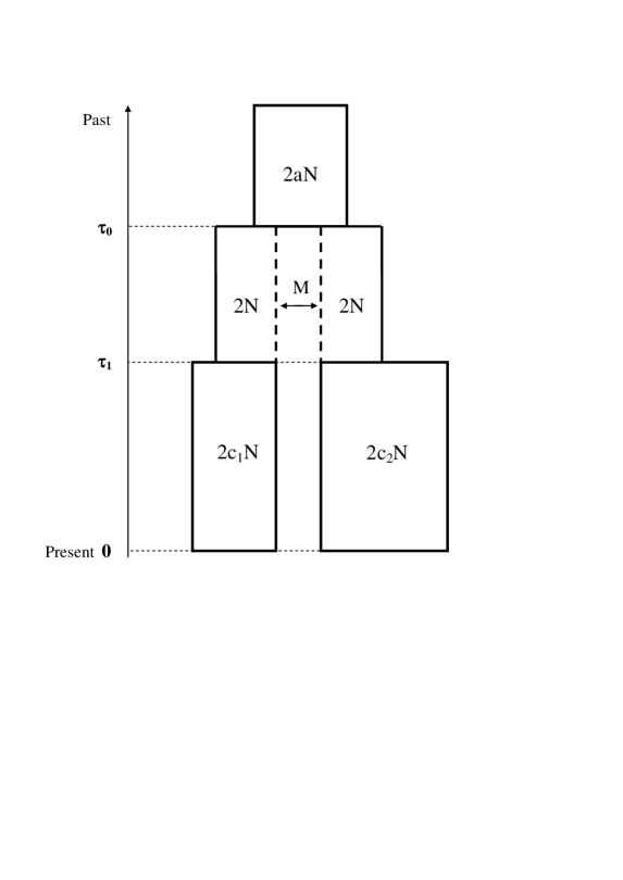
Figure 1: The “isolation with initial migration” (IIM) model.

Focusing on DNA sequences at a single locus that is not subject to intragenic recombination, the ancestral population is assumed to have been of constant size $2aN$ homologous sequences until the split occurred time $\tau_{0}$ ago, where $N$ is large. Between time $\tau_{0}$ ago and time $\tau_{1}$ ago, the two descendant populations were of constant size $2N$ sequences each and exchanged migrants at a constant rate $m$, where $m$ is the proportion of each descendant population that was replaced by immigrants each generation. The current size of descendant population $i$ is $2c_{i}N$ sequences ($i=1,2$), and is assumed to have been constant since migration ended time $\tau_{1}$ ago. As is standard in coalescent theory and assuming that reproduction within populations follows the neutral Wright-Fisher model, time is measured in units of $2N$ generations (this also applies to the times $\tau_{0}$ and $\tau_{1}$); in practical applications where the Wright-Fisher model does not hold, $N$ is interpreted as the effective population size. The “scaled” migration and mutation rates are defined as $M=4Nm$ and $\theta=4N\mu$, respectively, where $\mu$ is the mutation rate per DNA sequence per generation at the locus concerned. The work described in this paper assumes that mutations are selectively neutral and follow the infinite sites model (Watterson 1975). Extensions to other neutral mutation models are feasible but have not yet been implemented.

For this IIM model, Wilkinson-Herbots (2012) found the probability that two homologous DNA sequences differ at $k$ nucleotide sites: denoting by $S_{ij}$ the number of nucleotide differences between two homologous sequences sampled from descendant populations $i$ and $j$ ($i,j\in\{1,2\}$) and using the subscript $\theta$ to indicate the scaled mutation rate at the locus concerned, we have for $k=0,1,2,\ldots$

$$P_{\theta}(S_{ii}=k) = \frac{(c_{i}\theta)^{k}}{(1+c_{i}\theta)^{k+1}}\left(1-e^{-\tau_{1}(\frac{1}{c_{i}}+\theta)}\sum_{l=0}^{k}\frac{\left(\frac{1}{c_{i}}+\theta\right)^{l}\tau_{1}^{l}}{l!}\right)$$ (1)

$$\mbox{}+e^{-\frac{1}{c_{i}}\tau_{1}}\sum_{r=1}^{2}A_{0r}\frac{\lambda_{r}\theta^{k}}{(\lambda_{r}+\theta)^{k+1}}\left(e^{-\theta\tau_{1}}\sum_{l=0}^{k}\frac{(\lambda_{r}+\theta)^{l}\tau_{1}^{l}}{l!}-e^{-\lambda_{r}(\tau_{0}-\tau_{1})-\theta\tau_{0}}\sum_{l=0}^{k}\frac{(\lambda_{r}+\theta)^{l}\tau_{0}^{l}}{l!}\right)$$

$$\mbox{}+\frac{e^{-\frac{1}{c_{i}}\tau_{1}-\theta\tau_{0}}(a\theta)^{k}}{(1+a\theta)^{k+1}}\left(\sum_{l=0}^{k}\frac{\left(\frac{1}{a}+\theta\right)^{l}\tau_{0}^{l}}{l!}\right)\sum_{r=1}^{2}A_{0r}e^{-\lambda_{r}(\tau_{0}-\tau_{1})}$$

for a pair of sequences from the same descendant population, and

$$P_{\theta}(S_{12}=k) = \sum_{r=1}^{2}A_{1r}\frac{\lambda_{r}\theta^{k}}{(\lambda_{r}+\theta)^{k+1}}\left(e^{-\theta\tau_{1}}\sum_{l=0}^{k}\frac{(\lambda_{r}+\theta)^{l}\tau_{1}^{l}}{l!}-e^{-\lambda_{r}(\tau_{0}-\tau_{1})-\theta\tau_{0}}\sum_{l=0}^{k}\frac{(\lambda_{r}+\theta)^{l}\tau_{0}^{l}}{l!}\right)$$ (2)

$$\mbox{}+\frac{e^{-\theta\tau_{0}}(a\theta)^{k}}{(1+a\theta)^{k+1}}\left(\sum_{l=0}^{k}\frac{\left(\frac{1}{a}+\theta\right)^{l}\tau_{0}^{l}}{l!}\right)\sum_{r=1}^{2}A_{1r}e^{-\lambda_{r}(\tau_{0}-\tau_{1})}$$

for a pair of sequences from different descendant populations, where

$$\begin{array}[]{ll}\lambda_{1}={\displaystyle\frac{nM+n-1-\sqrt{D}}{2(n-1)}{}{}{}{}{}{}{}{}{}{}{}{}{}{}{}{}{}}&\lambda_{2}={\displaystyle\frac{nM+n-1+\sqrt{D}}{2(n-1)}}\end{array}$$

with

$$D=(nM+n-1)^{2}-4(n-1)M$$

and where

$$\begin{array}[]{ll}A_{01}={\displaystyle\frac{\lambda_{2}-1}{\lambda_{2}-\lambda_{1}}{}{}{}{}{}{}{}{}{}{}{}{}{}{}{}{}{}{}{}{}{}{}{}{}{}{}{}{}{}{}{}}&A_{02}={\displaystyle\frac{1-\lambda_{1}}{\lambda_{2}-\lambda_{1}}}\\ A_{11}={\displaystyle\frac{\lambda_{2}}{\lambda_{2}-\lambda_{1}}}&A_{12}={\displaystyle\frac{-\lambda_{1}}{\lambda_{2}-\lambda_{1}}}.\end{array}$$

Thus for pairwise difference data of the form $\{k_{l};l=1,\ldots,K\}$, consisting of the number of nucleotide differences between one pair of DNA sequences at each of $K$ independent loci, the likelihood under the IIM model is given by

$$\prod_{l=1}^{K}P_{\theta^{(l)}}(S_{i_{l}j_{l}}=k_{l})$$ (3)

where $i_{l}$ and $j_{l}$ denote the locations (i.e. the population labels) of the two DNA sequences sampled at the $l$th locus, and where each factor $P_{\theta^{(l)}}(S_{i_{l}j_{l}}=k_{l})$ is given by equation (1) or (2) as appropriate, replacing $\theta$ by the scaled mutation rate $\theta^{(l)}$ for the $l$th locus. Note that the above derivation of the likelihood assumes that there is no recombination within loci and free recombination between loci. In order to jointly estimate all the parameters of the model, data from between-population sequence comparisons as well as within-population sequence comparisons from both populations should be included in the above likelihood (where each pairwise comparison must be at a different, independent locus). The above explicit formula for the likelihood allows rapid computation and maximization, so that ML estimates can easily be obtained, as well as AIC scores and likelihood ratios comparing the IIM model with competing models such as the “complete isolation” model and the symmetric “isolation-with-migration” model. Similar ML methods were first developed by Takahata et al. (1995) for a number of different demographic models: a single population of constant size, a population undergoing an instantaneous change of size, and complete isolation models for two and for three species. Innan and Watanabe (2006) developed an extension of Takahata et al.’s MLE method to a more sophisticated model of gradual population divergence than the IIM model considered in this paper, but their calculation of the likelihood relies on numerical computation of the probability density function of the coalescence time using recursion equations on a series of time points (and then numerically integrating over the coalescence time to find the probability of $k$ nucleotide differences), which can be time-consuming; in addition, the accuracy of their recursion and likelihood calculation depend on the number of time points considered. The method described in the present paper assumes a simpler model than Innan and Watanabe’s, but is faster because both the calculation of the pdf of the coalescence time and the integration over the coalescence time to find the probability of $k$ nucleotide differences have already been done, in an exact way, to give equations (1) and (2) above, leaving far less computation to be done.

In order to obtain good starting values for the likelihood maximization under the IIM model, our implementation first fits a complete isolation model, as the latter model gives a more tractable likelihood surface and is therefore less sensitive to the choice of starting values. The parameter estimates obtained for the complete isolation model are then used as starting values to fit the IIM model; this was found to reduce the possibility that the program might otherwise converge on a local maximum rather than on the global maximum of the likelihood under the IIM model. Whilst the theoretical results obtained make it possible to directly compute ML estimates of the original parameters of the IIM model as described above ($\tau_{1},\tau_{0},c_{1},c_{2},a,M,\theta$), our implementation uses the following reparameterizations as this improved performance and robustness:

$$\begin{array}[]{l}T_{1}=\theta\tau_{1},\,\,V=\theta(\tau_{0}-\tau_{1}),\vspace*{2mm}\\ \theta_{1}=c_{1}\theta,\,\,\theta_{2}=c_{2}\theta,\,\,\theta_{a}=a\theta\end{array}$$ (4)

(similar to the choice of parameters in, for example, Yang 2002, and Hey and Nielsen 2004), i.e. $T_{1}$ and $V$ represent respectively the time since the end of gene flow and the duration of the period of gene flow, measured by twice the expected number of mutations per lineage during the period concerned; $\theta_{1},\theta_{2}$ and $\theta_{a}$ are the “population size parameters” of the current descendant populations and the ancestral population, respectively ($\theta=4N\mu$ is the population size parameter of each descendant population during the migration stage of the model). ML estimates are obtained jointly for the parameters $T_{1},V,\theta_{1},\theta_{2},\theta,\theta_{a},M$, and these can readily be converted to ML estimates of the original model parameters if required. Our computer code is included as Supplementary Material.

Equations (1) and (2) rely on the assumption of symmetric migration and equal population sizes during the period of gene flow. Without these assumptions, an explicit analytical formula for the likelihood becomes difficult to obtain. Simulation results suggest however that our method is reasonably robust to minor violations of these assumptions; furthermore, it is possible to extend our method to allow for asymmetric migration and unequal population sizes (Costa RJ and Wilkinson-Herbots HM, work in progress).

Results

Application to Drosophila data

To illustrate the MLE method for the IIM model described above, we applied this method to the genomic data set of D. simulans and D. melanogaster compiled and analyzed by Wang and Hey (2010), and reanalyzed by Lohse et al. (2011), who both used an IM model assuming a constant migration rate from the onset of speciation until the present. The data consist of alignments of 30,247 blocks of intergenic sequence of 500 bp each, from two inbred lines of D. simulans and from one inbred line each of D. melanogaster and D. yakuba, and have been pre-processed as described in Wang and Hey (2010) and Lohse et al. (2011). We also follow these authors in using D. yakuba as an outgroup to estimate the relative mutation rate at each locus. As our method uses the number of nucleotide differences between one pair of sequences at each locus, we had to choose two of the three sequences (which we will denote by D.sim1, D.sim2 and D.mel for brevity) at each locus. There are of course many ways in which this can be done (for example, one could choose two sequences at random at each locus, as done by Wang and Hey 2010). In order to use all the data, and to be able to check to what extent our results depend on our choice of sequences, we took the following approach: three (overlapping) pairwise data sets were formed by alternately assigning loci to the comparisons D.mel - D.sim1, D.mel - D.sim2 and D.sim1 - D.sim2, where data set 1 starts with D.mel - D.sim1 at locus 1 (D.mel - D.sim2 at locus 2, D.sim1 - D.sim2 at locus 3, and so on), data set 2 uses D.mel - D.sim2 at locus 1 (D.sim1 - D.sim2 at locus 2, …), and data set 3 starts with D.sim1 - D.sim2 at locus 1 (D.mel - D.sim1 at locus 2, …). Thus each sequence at each locus is used in exactly two of the three data sets, and each data set contains between-species differences at approximately 20,000 loci and within-species (D. simulans) differences at approximately 10,000 loci. ML estimates and estimated standard errors for the IIM model parameters $(T_{1},V,\theta_{1},\theta,\theta_{a},M)$ were obtained for each of the three data sets and then averaged over the three data sets. For comparison, in addition to fitting an IIM model as described above, we also obtained ML estimates assuming an IIM model with $\theta_{1}=\theta$ (or equivalently, $c_{1}=1$, i.e. not allowing for a change of population size at the end of the migration period), a symmetric IM model (which corresponds to putting $T_{1}=0$ in the IIM model), and a complete isolation model (which corresponds to assuming $M=0$ in addition to $T_{1}=0$; the size of descendant population 2 is irrelevant here). The results are given in Table 1.

Table 1: ML estimates, maximized loglikelihood ($\ln\hat{L}$), likelihood ratio test statistic ($\Lambda$) and AIC score, obtained by fitting the different models to the three sets of Drosophila sequence data.

data	model	$\hat{T}_{1}$	$\hat{V}$	$\hat{\theta}_{1}$	$\hat{\theta}$	$\hat{\theta}_{a}$	$\hat{M}$	$\ln\hat{L}$	$\Lambda$	AIC
set 1	isolation		13.66		5.67	4.69		-90,097.17	1,175.66	180,200.34
	IM		14.79		5.54	3.97	0.0209	-89,509.34	270.65	179,026.68
	IIM with $\theta_{1}=\theta$	5.87	9.99		5.47	3.48	0.1389	-89,374.01	518.43	178,758.03
	IIM	7.22	9.38	6.70	2.68	3.22	0.0888	-89,114.80		178,241.60
	(s.e.)	(0.20)	(0.16)	(0.11)	(0.12)	(0.09)	(0.0059)
set 2	isolation		13.57		5.72	4.77		-90,339.14	1,185.38	180,684.28
	IM		14.80		5.58	3.98	0.0227	-89,746.45	347.39	179,500.90
	IIM with $\theta_{1}=\theta$	6.27	9.88		5.49	3.37	0.1793	-89,572.76	685.95	179,155.51
	IIM	7.62	9.43	6.85	2.31	3.05	0.0904	-89,229.78		178,471.56
	(s.e.)	(0.17)	(0.15)	(0.11)	(0.11)	(0.09)	(0.0054)
set 3	isolation		13.63		5.59	4.72		-89,979.56	1,094.44	179,965.12
	IM		14.69		5.48	4.04	0.0193	-89,432.34	291.86	178,872.68
	IIM with $\theta_{1}=\theta$	6.29	9.67		5.39	3.46	0.1635	-89,286.41	548.28	178,582.82
	IIM	7.31	9.31	6.62	2.56	3.23	0.0870	-89,012.27		178,036.54
	(s.e.)	(0.20)	(0.16)	(0.11)	(0.12)	(0.09)	(0.0058)
average	IIM	7.39	9.38	6.72	2.52	3.16	0.0887
	(s.e.)	(0.19)	(0.15)	(0.11)	(0.11)	(0.09)	(0.0057)

NOTE – The values of the likelihood ratio test statistic $\Lambda$ shown are for the comparison of the model concerned (considered to be the null model) against the model immediately underneath it. Estimated standard errors (numbers in brackets) are provided for the model with the best fit, i.e. the full IIM model. The bottom section of the table gives the parameter estimates under the IIM model, averaged over the three data sets; for each parameter, the average of the estimated standard errors for the three data sets is given in brackets, which serves as an estimated upper bound on the standard error of the averaged parameter estimate (estimates of the exact standard errors would be hard to obtain as the three data sets overlap).

Fitting the full IIM model took approximately 20 seconds for each of the three data sets, on a desktop PC. Estimated mutation rates, and hence the estimates of the parameters $T_{1},V,\theta_{1},\theta$ and $\theta_{a}$ defined in (4), are averages over all the loci considered. Mutation rate heterogeneity between loci was accounted for by estimating the relative mutation rate at each locus from comparison with the outgroup D. yakuba, as proposed in Wang and Hey (2010) (see “Materials and Methods” for further details); for simplicity these relative mutation rates are treated as known constants (see also Yang 1997, 2002), i.e. uncertainty about the relative mutation rates is ignored. Table 2 shows the estimates (averages over the three data sets) converted to times in years, diploid effective population sizes, and the migration rate per generation, for each of the four models considered.

Table 2: ML estimates of D. simulans - D. melanogaster divergence times, effective population sizes and migration rate per generation, under the different models considered, obtained with the full sequence data.

model	$\hat{t}_{1}$	$\hat{t}_{0}$	$\hat{N}_{1}$	$\hat{N}$	$\hat{N}_{a}$	$\hat{m}$
isolation		2.97my		6.18m	5.16m
IM		3.22my		6.04m	4.36m	$8.68\times 10^{-10}$
IIM with $c_{1}=1~{}~{}~{}~{}~{}$	1.34my	3.49my		5.95m	3.75m	$6.75\times 10^{-9}$
IIM	1.61my	3.66my	7.33m	2.75m	3.45m	$8.11\times 10^{-9}$
(s.e.)	(0.04my)	(0.03my)	(0.12m)	(0.12m)	(0.10m)	($0.59\times 10^{-9}$)

NOTE – The abbreviations “my” and “m” stand for “million years” and “million individuals”. The times $t_{1}$ and $t_{0}$ denote, respectively, the time since complete isolation of D. simulans and D. melanogaster (for the IIM model), and the time since the onset of speciation (for all models), i.e. these are the times $\tau_{1}$ and $\tau_{0}$ converted into years (see Fig.1). $N$ denotes the effective size of D. simulans in the isolation and IM models, and during the migration stage of the IIM model; $N_{1}=c_{1}N$ denotes the present effective size of D. simulans in the full IIM model; $N_{a}=aN$ is the effective size of the ancestral population. The estimates shown are the averages of the estimates obtained for the three (overlapping) data sets described in the text. For the IIM model, the averaged estimated standard error is also given (in brackets) for each parameter; this is an estimated upper bound on the standard error of the averaged parameter estimate.

These conversions assume a generation time of 0.1 year and a 10 million year speciation time between D. yakuba and D. melanogaster/D. simulans (as assumed by Wang and Hey 2010, and by Lohse et al. 2011; see also Powell 1997). It is seen that the IIM model places the onset of speciation ($\hat{t}_{0}=3.66$ million years) further back into the past than both the isolation model and the IM model, whereas the estimated time since complete isolation of the two species under the IIM model ($\hat{t}_{1}=1.61$ million years) is more recent than under the isolation model. Under the IIM model we obtain an estimated ancestral effective population size of $3.45$ million individuals, splitting into two populations containing $2.75$ million individuals each during the time interval when gene flow occurred, with D. simulans expanding to a current effective population size of $7.33$ million individuals. Note that the estimated migration rate per generation ($\hat{m}$) is an order of magnitude higher under the IIM model than under the IM model.

On the one hand, our averaging of the estimated standard errors over the three data sets (bottom rows of Tables 1 and 2) will have given us an overestimate of the standard error of the averaged parameter estimates. On the other hand, however, it should be noted that these estimated standard errors underrepresent the true total amount of uncertainty, as they do not account for uncertainty about the relative mutation rates at the different loci (which have been treated as known constants, whereas in practice we have estimated them from comparison with D. yakuba). Care should be taken therefore in the interpretation of the estimated standard errors stated in Tables 1 and 2.

Table 1 also gives the maximized loglikelihood ($\ln\hat{L}$) for the different models fitted, for each of the three data sets. It is seen that, amongst the models being compared, the full IIM model consistently gives by far the best loglikelihood value, though of course this model also has the largest number of parameters. The easiest way of comparing the fit of the different models is by using Akaike’s Information Criterion, AIC, which was designed to compare competing models with different numbers of parameters (AIC scores were also used in, for example, Takahata et al. 1995, Nielsen and Wakeley 2001, and Carstens et al. 2009). For each model (and for the same data), AIC is defined as

$$\mbox{AIC}=-2\ln\hat{L}+2\times\mbox{number of independently adjusted parameters within the model}$$

(Akaike 1972, 1974). Thus a larger maximized likelihood leads to a lower AIC score, subject to a penalty for each additional model parameter. The “Minimum AIC Estimate” (MAICE) is then defined by the model (and the Maximum Likelihood estimates of the model parameters) which gives the smallest AIC value amongst the competing models considered. Table 1 includes, for each data set, the AIC scores of the different models considered. It is seen that for each of the three data sets, the MAICE is given by the full IIM model. Thus, out of all the models considered here, the IIM model provides the best fit to the data, as measured by the AIC scores. The results in Table 1 also show that an IIM model with $\theta_{1}=\theta$ has a substantially better AIC score than a symmetric IM model, suggesting that the improved fit of the IIM model compared to the IM model is indeed due at least in part to accounting for the eventual complete isolation of the two species, and is not due solely to allowing differences between population sizes.

An alternative approach is to perform a series of likelihood ratio tests for nested models (see, for example, Cox 2006, Section 6.5 on “Tests and model reduction”). Focusing on any one of the three data sets in Table 1, if we start with the full IIM model and look upwards, each of the models considered reduces to the model immediately above it by fixing the value of one parameter: respectively $\theta_{1}=\theta$, $T_{1}=0$, and $M=0$. Each pair of “neighbouring” models can then be formally compared by means of a likelihood ratio test, where the null hypothesis represents the simpler of the two models (i.e. the one with fewer free parameters). If the null hypothesis is true, then the test statistic

$$\Lambda=2\times\left(\ln\hat{L}(\mbox{alternative model})-\ln\hat{L}(\mbox{null model})\right)$$

should approximately follow a $\chi^{2}_{1}$ distribution if the “null” value of the parameter concerned is an interior point of the parameter space (as is the case when we test $\theta_{1}=\theta$), whereas we might expect $\Lambda$ to follow approximately a $\frac{1}{2}\times 0+\frac{1}{2}\times\chi^{2}_{1}$ mixture if the “null” value of the parameter concerned lies on the boundary of the parameter space (as is the case in the tests of $T_{1}=0$ and $M=0$); using a $\chi^{2}_{1}$ distribution in the latter case is conservative (Self and Liang 1987; see also our simulation results below). The value of the likelihood ratio test statistic $\Lambda$ is given in Table 1 for each possible null model, when evaluated against the model immediately underneath it. For each model comparison, the value of the test statistic $\Lambda$ is so large that the simpler model is rejected in favour of the more complex model underneath it, with, in each case, a very small p-value ($p<<10^{-10}$) providing overwhelming evidence against the simpler model. Thus these likelihood ratio tests also identify the full IIM model as the most plausible amongst the different models considered.

Simulation results

Simulations were done to assess how well our method performs and how reliable the estimates obtained in the previous section are. From the three pairwise sets of Drosophila sequence data considered in Table 1, we arbitrarily selected the first one (“data set 1”) and mimicked this data set in our simulations.

Simulations from the IIM model

Each simulated data set consists of the number of nucleotide differences between a pair of DNA sequences sampled from descendant population 1 for 10,082 independent loci, and the number of differences between a pair of DNA sequences taken from different descendant populations for 20,165 independent loci, generated under the full IIM model with “true” parameter values equal to the estimates obtained for data set 1 (i.e. $T_{1}=7.22$, $V=9.38$, $\theta_{1}=6.70$, $\theta=2.68$, $\theta_{a}=3.22$ and $M=0.0888$) and the infinite sites model of neutral mutation. These numbers of loci for both types of comparison match those in Drosophila data set 1, and so do the relative mutation rates assumed at the different loci. One hundred such data sets were generated. For each simulated data set, ML estimates of the parameters were obtained using our R program for the IIM model, i.e. the method described in “New Approaches”. The resulting estimates are shown in Figure 2.

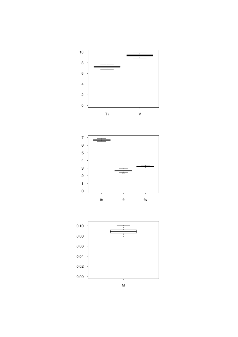
Figure 2: ML estimates obtained for 100 simulated data sets. The simulations assumed an IIM model with true parameter values $T_{1}=7.22$, $V=9.38$, $\theta_{1}=6.70$, $\theta=2.68$, $\theta_{a}=3.22$ and $M=0.0888$. Each simulated data set consists of the number of nucleotide differences between two DNA sequences from descendant population 1 at 10,082 independent loci, and between two DNA sequences from different descendant populations at 20,165 independent loci. Different loci were assumed to have different mutation rates: the relative mutation rates used at the different loci match those of the Drosophila data considered in this paper.

As one would expect, it is seen that (at least for a large sample size) our ML estimation procedure gives estimates centred on, and close to, the “true” parameter values.

In order to assess whether our method enables us to correctly select the IIM model from amongst the different models considered, when the IIM model is in fact the true underlying model, we also mimicked the type of analysis as was shown for data set 1 in Table 1: for each simulated data set, we fitted an isolation model, a symmetric IM model, an IIM model with $\theta_{1}=\theta$, and a full IIM model, and computed the AIC scores and the values of the likelihood ratio test statistic $\Lambda$. Both procedures (using AIC scores or likelihood ratio tests) correctly identified the full IIM model as the best-fitting model, for each of the 100 simulated data sets. The smallest difference obtained between the AIC scores of any two neighbouring models was in fact $242.96$, with the simpler model always having the worse AIC score, and the smallest difference observed between the AIC scores of the full IIM model and any other model was $409.93$, indicating that the IIM model could be identified with ease. For the likelihood ratio approach, comparing the value of the test statistic $\Lambda$ for a pair of neighbouring models with the $\chi^{2}_{1}$ distribution gave in all cases a $p$-value much smaller than $10^{-10}$, providing extremely strong evidence against the simpler of the two models compared (the smallest value of $\Lambda$ obtained for any pair of neighbouring models was $244.96$, whereas the $(1-10^{-10})$ quantile of the $\chi^{2}_{1}$ distribution is only $41.82$). When comparing the full IIM model directly with the isolation model by means of a likelihood ratio test, the smallest value of $\Lambda$ observed amongst the simulated data sets was $1158.40$, again giving a $p$-value very much smaller than $10^{-10}$ (using the $\chi^{2}_{3}$ distribution) for each of the 100 simulated data sets.

Simulations from the isolation model

We also simulated 100 data sets under the isolation model, to further investigate the performance of our method in identifying the correct model, and whether false positives may be produced – in particular, whether a signal of gene flow may be obtained when in reality there was no gene flow. The “true” parameter values assumed in the simulations were those obtained from fitting an isolation model to Drosophila data set 1 (see Table 1). Two of the simulated data sets were problematic, in that only the isolation model could be fitted: due to some large values ($>200$) for the simulated numbers of nucleotide differences between pairs of sequences from different species, R was unable to evaluate the likelihood for any of the other models in the relevant part of the parameter space. For the remaining $98$ simulated data sets for which all models could be fitted, a likelihood ratio test using as the null distribution the naive $\chi^{2}$ distribution (with degrees of freedom equal to the difference between the number of parameters in the two models being compared) gave better results than did comparison of AIC scores. On the basis of AIC scores, an incorrect model was selected for as many as 19 of the simulated data sets: in 6 cases the IM model gave the lowest AIC score, in 2 cases the IIM model with $\theta_{1}=\theta$, and in 11 cases the full IIM model. However, in 6 of the 11 cases where the full IIM model was selected, the estimated migration rate was $0$ so that this “IIM” model was in fact an isolation model but with an additional small change of population size.

A likelihood ratio test of the isolation model against the IM model at a significance level of $1\%$ resulted in acceptance of the isolation model for all 98 data sets, regardless of whether we used $\chi^{2}_{1}$ or $(\frac{1}{2}\times 0+\frac{1}{2}\times\chi^{2}_{1})$ as the null distribution. At a significance level of $5\%$, the isolation model was rejected for 4 of the 98 simulated data sets if we used $\chi^{2}_{1}$, and for 6 of the simulated data sets if the mixed $\chi^{2}$ distribution was used. Figure 3

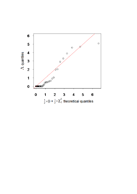
Figure 3: QQ-plot of the likelihood ratio test statistic $\Lambda=2\times(\ln\hat{L}(\mbox{IM})-\ln\hat{L}(\mbox{isolation}))$ against the $\chi^{2}_{1}$ distribution (left), and against the mixture $\frac{1}{2}\times 0+\frac{1}{2}\times\chi^{2}_{1}$ (right). On the vertical axis we have plotted the sample quantiles of the values of $\Lambda$ observed when testing the isolation model against the IM model for $100$ data sets simulated from the isolation model (2 data sets have been omitted as R was unable to fit the IM model - please see the main text for further details). The line $y=x$ is also shown for ease of comparison.

shows that the use of $\chi^{2}_{1}$ as the null distribution is indeed conservative, and suggests that this may be preferable to using the mixed $\chi^{2}$ distribution.

Similarly, at a significance level of $1\%$, a likelihood ratio test of the isolation model against the IIM model with $\theta_{1}=\theta$ led to acceptance of the isolation model for all 98 data sets, whether we used $\chi^{2}_{2}$ or the mixture $(\frac{1}{4}\times 0+\frac{1}{2}\times\chi^{2}_{1}+\frac{1}{4}\times\chi^{2}_{2})$ as the null distribution. At a significance level of $5\%$, the use of $\chi^{2}_{2}$ resulted in rejection of the isolation model for 1 of the 98 data sets, whilst the use of $(\frac{1}{4}\times 0+\frac{1}{2}\times\chi^{2}_{1}+\frac{1}{4}\times\chi^{2}_{2})$ as the null distribution led to rejection of the isolation model for 5 of the data sets. The QQ-plots shown in Figure 4 confirm again that the use of $\chi^{2}_{2}$ in this case is conservative.

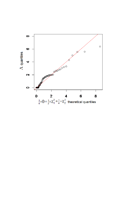
Figure 4: QQ-plot of the likelihood ratio test statistic $\Lambda=2\times(\ln\hat{L}(\mbox{IIM with $\theta_{1}=\theta$})-\ln\hat{L}(\mbox{isolation}))$ against the $\chi^{2}_{2}$ distribution (left), and against the mixture $\frac{1}{4}\times 0+\frac{1}{2}\times\chi^{2}_{1}+\frac{1}{4}\times\chi^{2}_{2}$ (right). On the vertical axis we have plotted the sample quantiles of the values of $\Lambda$ observed when testing the isolation model against the IIM model with $\theta_{1}=\theta$ for $100$ data sets simulated from the isolation model (2 data sets have been omitted as R was unable to fit the IIM model with $\theta_{1}=\theta$). The line $y=x$ is also shown for ease of comparison.

Similarly, the QQ-plots in Figure 5 indicate that the use of the $\chi^{2}_{3}$ distribution is conservative when testing the isolation model against the full IIM model, and that this may be preferable to the use of a mixed $\chi^{2}$ distribution. A likelihood ratio test at a significance level of $1\%$ led to acceptance of the isolation model for all 98 data sets if a $\chi^{2}_{3}$ distribution was used, and resulted in rejection of the isolation model for 1 of the 98 data sets when using the mixed $(\frac{1}{4}\times\chi^{2}_{1}+\frac{1}{2}\times\chi^{2}_{2}+\frac{1}{4}\times\chi^{2}_{3})$ distribution. At a significance level of $5\%$, using the $\chi^{2}_{3}$ distribution resulted in rejection of the isolation model for 4 of the 98 data sets (in 2 of these 4 cases the estimated migration rate was $0$, reducing the IIM model to an isolation model with an additional slight change of population size), whereas the use of the mixed $\chi^{2}$ distribution led to rejection of the isolation model for 12 of the 98 data sets (in 6 of these 12 cases, the estimated migration rate was $0$).

Figure 5: QQ-plot of the likelihood ratio test statistic $\Lambda=2\times(\ln\hat{L}(\mbox{IIM})-\ln\hat{L}(\mbox{isolation}))$ against the $\chi^{2}_{3}$ distribution (left), and against the mixture $\frac{1}{4}\times\chi^{2}_{1}+\frac{1}{2}\times\chi^{2}_{2}+\frac{1}{4}\times\chi^{2}_{3}$ (right). On the vertical axis we have plotted the sample quantiles of the values of $\Lambda$ obtained when testing the isolation model against the full IIM model for $100$ data sets simulated from the isolation model (2 data sets have been omitted as R was unable to fit the IIM model). The line $y=x$ is also shown for ease of comparison.

Discussion

In this paper we have presented a very fast method to obtain ML estimates and to distinguish between different evolutionary scenarios, using nucleotide difference data from pairs of sequences at a large number of independent loci. The IIM model considered allows for an initial period of gene flow between two diverging populations or species, followed by a period of complete isolation, and is more appropriate in the context of speciation than the IM model commonly used in the literature (which assumes that gene flow continues at a constant rate all the way until the present time). We have illustrated the speed and power of our method by applying it to a large data set from two related species of Drosophila, and to simulated data. Fitting an IIM model to a data set of approximately 30,000 loci (with an average length of about 400 bp and varying mutation rates) from two species of Drosophila took approximately 20 seconds on a desktop PC; this time included fitting an isolation model first in order to obtain good starting values for the parameters. Moreover, the results made it possible to distinguish between more and less plausible models (representing alternative evolutionary scenarios) with ease, and identified the IIM model as providing the best fit amongst the models considered.

The Drosophila data set studied in this paper was previously analysed by Wang and Hey (2010), who compiled the data, and by Lohse et al. (2011). Both fitted IM models to these data, assuming that gene flow occurred at a constant rate from the time of separation of the two species until the present time. In Tables 1 and 2, alongside our results for the IIM model, we also included parameter estimates for a symmetric IM model, for the sake of comparison. As expected, our IM results are in close agreement with those of Lohse et al. (2011), who fitted two versions of the IM model, one with symmetric migration and one with migration in only one direction (D. simulans to D. melanogaster forward in time, motivated by Wang and Hey’s results). They found that their estimated migration rate for the symmetric model is approximately half that obtained for the model with migration in one direction, i.e. both models gave the same estimated total number of migrants per generation between the two species in the two directions combined, whereas their estimates of the other parameters are virtually identical for the two models (see p.23 of their Supporting Information). Our IM results are also in good agreement with those of Wang and Hey (2010), even though they fitted a more general version of the IM model (allowing for unequal sizes of the two species and unequal migration rates in the two directions) and assumed the Jukes-Cantor model of mutation, whereas our results and those of Lohse et al. (2011) assume the infinite sites model for its mathematical simplicity. Indeed, Lohse et al. (2011) comment on how little difference the assumption of the infinite sites model makes to the IM results for the pairwise Drosophila data, compared to Wang and Hey’s results based on the Jukes-Cantor model. Of more interest is the comparison of these authors’ IM results with those obtained for our IIM model. We note firstly that their estimates of 3.04 million years (Wang and Hey 2010) or 2.98 million years (Lohse et al. 2011) for the simulans-melanogaster speciation time, and also our IM estimate of 3.22 million years, fall in between our IIM estimates of 3.66 million years for the time since the onset of speciation ($t_{0}$) and 1.61 million years for the time since complete isolation of these two species ($t_{1}$). Secondly, under the IM model the amount of gene flow between the two species (in the two directions combined) was estimated at 0.0134 migrant gene copies per generation (Wang and Hey 2010), 0.0255 migrant gene copies per generation (Lohse et al. 2011, asymmetric IM model), 0.0256 (Lohse et al. 2011, symmetric IM model), or 0.0210 migrant gene copies per generation (our IM results in Table 1, averaged over the three data sets). These estimates are considerably smaller than the corresponding estimate of 0.0887 migrant gene copies per generation during the period of migration under our IIM model.

Lohse et al. (2011) also considered a trimmed version of the Wang and Hey (2010) Drosophila data, where they shortened all loci to a fixed number of nucleotide differences between D. melanogaster and the D. yakuba outgroup, so that the estimated mutation rate for all loci was equal. This assumption that all loci have the same mutation rate massively speeds up the computation of the likelihood, since in this case the probability of $k$ differences needs to be calculated only once for each observed value of $k$, rather than having to calculate this probability over and over again for different mutation rates at different loci. Further to this idea, we also implemented a simplified, much faster, version of our MLE method to be used for data sets where all loci have the same mutation rate (this R code is also included as Supplementary Material). Applying this version of our IIM program to the trimmed Drosophila data (still approximately 30,000 loci) gave virtually instant results on a desktop PC, i.e. the computing time was $<<1$ second. However, the substantial shortening of loci did result in loss of information, and the distinction between more and less plausible models was not always as clear anymore, as the differences between the values of the maximized loglikelihood for the different models (and hence the values of the likelihood ratio test statistic $\Lambda$, and the differences between the AIC scores of different models) were not as large as they were for the full sequence data. Nevertheless, the full IIM model could still be identified as giving the best fit amongst the models considered in this paper, both on the basis of AIC scores and by means of likelihood ratio tests. Table 3 gives the estimates obtained by fitting the IIM model to the trimmed data; the conversion to times in years, diploid effective population sizes and migration rate per generation was done using a generation time of 0.1 year and a 10 million year speciation time between D. yakuba and {D. melanogaster, D. simulans}, as before. The results are broadly in agreement with the corresponding estimates for the full sequence data (see Table 2, bottom row).

Table 3: ML estimates of D. simulans - D. melanogaster divergence times, effective population sizes and migration rate per generation, under the full IIM model, obtained with the trimmed sequence data.

model	$\hat{t}_{1}$	$\hat{t}_{0}$	$\hat{N}_{1}$	$\hat{N}$	$\hat{N}_{a}$	$\hat{m}$
IIM	1.52my	3.67my	6.04m	3.94m	3.82m	$11.27\times 10^{-9}$
(s.e.)	(0.16my)	(0.10my)	(0.11m)	(0.33m)	(0.18m)	($2.89\times 10^{-9}$)

NOTE – The abbreviations “my” and “m” stand for “million years” and “million individuals”. The times $t_{1}$ and $t_{0}$ denote, respectively, the time since complete isolation of D. simulans and D. melanogaster, and the time since the onset of speciation, i.e. these are the times $\tau_{1}$ and $\tau_{0}$ converted into years (see Fig.1). The effective population sizes $N_{1}$, $N$ and $N_{a}$ refer respectively to the present D. simulans population, each population during the migration stage of the model, and the ancestral population. The estimates shown have been averaged over the three overlapping data sets described in the text. The averaged estimated standard error is also given (in brackets) for each parameter; this is an estimated upper bound on the standard error of the averaged parameter estimate.

The purpose of our analysis of the Drosophila data was merely to illustrate the potential of our method, rather than to draw any firm conclusions about the evolutionary history of the particular species concerned. Whilst the IIM model provides the best fit to the Drosophila data amongst the different models considered in this paper, it is likely that more realistic models can be constructed which provide yet a better fit than the version of the IIM model considered here. Our assumption of equal population sizes and symmetric migration during the period of gene flow in the model is obviously an unrealistic oversimplification, but was made for the sake of mathematical tractability and computational speed. An extension of our method to a more general IIM model allowing for unequal migration rates and unequal population sizes during the migration stage of the model is possible and is being developed (Costa RJ and Wilkinson-Herbots HM, work in progress). Similarly, the current implementation of our method assumes the infinite sites model of neutral mutation because of its mathematical ease. Extensions of our method to other neutral mutation models (for example, the Jukes-Cantor model) can be done but have not yet been implemented. It should also be feasible to extend our method to incorporate more than two species.

Whilst our method explicitly allows for mutation rate heterogeneity between loci (whether due to variation in sequence length or variation in the mutation rate per site, or both), our current implementation assumes that accurate estimates of the relative mutation rates of the different loci are available (our implementation treats the relative mutation rates as known constants). This limitation will become less important as more and more genome sequences become available, allowing more accurate estimation of the relative mutation rates. For our analysis of the Drosophila data presented in this paper, however, the relative mutation rates of the different loci were estimated by comparison of {D. simulans, D. melanogaster} with the outgroup D. yakuba, as was done also by Wang and Hey (2010) and by Lohse et al. (2011). Using more than one outgroup sequence (if available) to estimate the relative mutation rate at each locus should improve the accuracy. It may also be possible to adapt our method to incorporate uncertainty about the relative mutation rates by modelling mutation rate variation as a random variable and integrating out over it (see Yang 1997, or the “all-rate” method proposed by Wang and Hey 2010).

Materials and Methods

The Drosophila data considered in this paper are the D. melanogaster - D. simulans divergence data compiled and analyzed by Wang and Hey (2010); we used the subset of the data that was studied also by Lohse et al. (2011). The data consist of alignments of 30,247 segments of intergenic sequence of length 500 bp each, from two inbred lines of D. simulans and one inbred line of D. melanogaster, and from an inbred line of D. yakuba for use as an outgroup. The data have been pre-processed as described in Wang and Hey (2010) and Lohse et al. (2011); the version of the data used is that labelled “WangHeyRaw” in the Supporting Information of Lohse et al. (2011). As our method uses pairwise nucleotide differences, subsets of the data were formed by selecting one pair of sequences from each locus (i.e. D.mel - D.sim1, D.mel - D.sim2, or D.sim1 - D.sim2). Three such subsets were formed as described in the Section on “Results”; these three data sets overlap as each sequence at each locus is used in two of the three data sets. Parameter estimates and estimated standard errors were obtained for each of these three data sets separately and then averaged over the three data sets. This gives too large estimates of the standard errors of the averaged parameter estimates; however, due to the overlap between the data sets, more accurate estimated standard errors would be difficult to obtain.

Following Wang and Hey (2010) and Lohse et al. (2011), mutation rate heterogeneity between loci was accounted for by comparing the D. melanogaster and D. simulans sequences with the outgroup D. yakuba. Calculating the outgroup divergence $d_{l}$ between {D. simulans, D. melanogaster} and D. yakuba at locus $l$ as a weighted average over the available sequences, assigning 25% weight to each of the simulans sequences and 50% weight to the single melanogaster sequence, the relative mutation rate $r_{l}$ of locus $l$ was estimated as $r_{l}=d_{l}/\bar{d}$, where $\bar{d}$ is the average of the $d_{l}$ over all loci. The scaled mutation rate at locus $l$ is then given by $\theta^{(l)}=r_{l}\theta$, where $\theta$ is the average scaled mutation rate over all the loci considered. The relative mutation rates $r_{l}$ are treated as fixed constants in the likelihood maximization (see also Yang 1997, 2002).

Estimates of the parameters of the IIM model were obtained by maximizing the likelihood, given by equation (3), using the reparameterization (4). In order to obtain reasonable starting values for the likelihood maximization under the IIM model, it can be helpful to first fit an isolation model, as the latter has a more tractable likelihood surface. Estimated standard errors are obtained from the inverted Hessian matrix. The computer code was written in R and is included as Supplementary Material. Table 1 shows the results obtained for the three sets of Drosophila data.

To convert the parameter estimates into readily interpretable units, we followed Wang and Hey (2010) and Lohse et al. (2011) in using a generation time of $g=0.1$ year and a 10 million year speciation time between D. yakuba and {D. simulans, D. melanogaster} (see also Powell 1997), which gives us an estimate of $\bar{\mu}=2.29\times 10^{-7}$ for the mutation rate per locus per generation, averaged over all the loci included in the analysis. The converted estimates given in Table 2 were then calculated according to the following equations:

$$t_{1} = T_{1}\times\frac{g}{2\bar{\mu}}$$

$$t_{0} = (T_{1}+V)\times\frac{g}{2\bar{\mu}}$$

for the times in years since complete isolation and since the onset of speciation, respectively;

$$N=\frac{\theta}{4\bar{\mu}}$$

for the effective size (number of diploid individuals) of either population during the migration stage of the model, and similarly for all other population sizes; and

$$m=\frac{M}{\theta}\times\bar{\mu}$$

for the migration rate per generation. Estimated standard errors for the converted estimates were obtained by re-running a reparameterized version of the program, in terms of $T_{0}=T_{1}+V$ and $\Psi=\frac{M}{\theta}$ instead of $V$ and $M$, using the ML estimates already obtained as starting values, allowing easy computation of the Hessian matrix. As before, estimated standard errors were computed separately for each of the three data sets and then averaged.

Following Lohse et al. (2011) we also analyzed a trimmed version of the Wang and Hey (2010) Drosophila data, where each locus was cut after 16 nucleotide differences between D. melanogaster and D. yakuba, and the remainder of the locus was ignored; the 2,090 loci which had fewer than 16 differences between D. melanogaster and D. yakuba were omitted altogether, leaving 28,157 trimmed loci for analysis. This trimming amounts to a shortening of the loci by roughly a factor of 3 on average. Again, three (overlapping) subsets of the data were formed, each containing one pair of sequences from each locus (i.e. D.mel - D.sim1, D.mel - D.sim2, or D.sim1 - D.sim2) as described above and in the Section on “Results”. Parameter estimates and estimated standard errors were obtained for each of these three data sets separately and then averaged over the three data sets. We used a simplified version of our R code written specifically for data sets where all loci have the same estimated mutation rate; this simplified code is also included as Supplementary Material. The likelihood calculation uses the frequencies of the observed numbers of pairwise differences, which is much faster than the corresponding code for the case where different loci have different mutation rates: for the trimmed Drosophila data, instead of evaluating 28,157 terms in the loglikelihood (one term for each locus), only about 50 different terms need to be calculated (corresponding to the different values of the number of pairwise differences observed, within and between species) and multiplied by their frequencies, which hugely speeds up the likelihood computation and maximization. Table 3 shows the results obtained under the IIM model, after conversion into conventional units as explained above, using a mutation rate of $\mu=8\times 10^{-8}$ per locus per generation for the trimmed data (see also Lohse et al 2011).

Simulated pairwise difference data were generated by first simulating the coalescence times of pairs of sequences and then superimposing neutral mutation under the infinite sites model; our R code is included as Supplementary Material. For pairs of sequences from the same species, our simulation algorithm uses the “shortcut” provided by equations (8) and (9) in Wilkinson-Herbots (2012), exploiting the fact that the distribution of the coalescence time of a pair of sequences sampled from the same species in the IIM model is a mixture of two “piecewise exponential” distributions (with “change points” $\tau_{1}$ and $\tau_{0}$), eliminating the need to explicitly simulate migration events.

Supplementary Material

The R code which fits an IIM model and an isolation model to pairwise difference data from a large number of independent loci is supplied as Supplementary Material. The R code for simulating pairwise difference data under the IIM model is also provided.

References

Akaike H. 1972. Information theory and an extension of the maximum likelihood principle. In: Petrov BN, Csaki F, editors. Proc. 2nd Int. Symp. Information Theory, Supp. to Problems of Control and Information Theory. p. 267-281.

Akaike H. 1974. A new look at the statistical model identification. IEEE Transactions on Automatic Control AC-19:716-723.

Andersen LN, Mailund T, Hobolth A. 2014. Efficient computation in the IM model. J Math Biol. 68:1423-51.

Becquet C, Przeworski M. 2007. A new approach to estimate parameters of speciation models with application to apes. Genome Res. 17:1505-1519.

Becquet C, Przeworski M. 2009. Learning about modes of speciation by computational approaches. Evolution 63:2547-2562.

Bird CE, Fernandez-Silva I, Skillings DJ, Toonen RJ. 2012. Sympatric speciation in the post “modern synthesis” era of evolutionary biology. Evol Biol. 39:158-180.

Burgess R, Yang Z. 2008. Estimation of hominoid ancestral population sizes under Bayesian coalescent models incorporating mutation rate variation and sequencing errors. Mol Biol Evol. 25:1979-1994.

Carstens BC, Stoute HN, Reid NM. 2009. An information-theoretical approach to phylogeography. Mol Ecol 18:4270-4282.

Cox DR. 2006: Principles of Statistical Inference. Cambridge University Press.

Hey J. 2005. On the number of New World founders: a population genetic portrait of the peopling of the Americas. PLoS Biol. 3:965-975.

Hey J. 2010. Isolation with migration models for more than two populations. Mol Biol Evol 27:905-920.

Hey J, Nielsen R. 2004. Multilocus methods for estimating population sizes, migration rates and divergence time, with applications to the divergence of Drosophila pseudoobscura and D. persimilis. Genetics 167:747-760.

Hey J, Nielsen R. 2007. Integration within the Felsenstein equation for improved Markov Chain Monte Carlo methods in population genetics. Proc Natl Acad Sci USA. 104:2785-2790.

Hobolth A, Andersen LN, Mailund T. 2011. On computing the coalescence time density in an isolation-with-migration model with few samples. Genetics 187:1241-1243.

Innan H, Watanabe H. 2006. The effect of gene flow on the coalescent time in the human-chimpanzee ancestral population. Mol Biol Evol. 23:1040-1047.

Li H, Durbin R. 2011. Inference of human population history from individual whole-genome sequences. Nature 475(7357):493-496.

Lohse K, Sharanowski B, Stone GN. 2010. Quantifying the Pleistocene history of the oak gall parasitoid cecidostiba fungosa using twenty intron loci. Evolution 64:2664-2681.

Lohse K, Harrison RJ, Barton NH. 2011. A general method for calculating likelihoods under the coalescent process. Genetics 189:977-987.

Maddison WP, Knowles LL. 2006. Inferring phylogeny despite incomplete lineage sorting. Syst Biol. 55:21-30.

Nadachowska K. 2010. Divergence with gene flow - the amphibian perspective. Herpetological Journal 20:7-15.

Nielsen R, Wakeley J. 2001. Distinguishing migration from isolation: a Markov Chain Monte Carlo approach. Genetics 158:885-896.

Pinho C, Hey J. 2010. Divergence with gene flow: models and data. Annu Rev Ecol Evol Syst. 41:215-230.

Powell JR. 1997. Progress and Prospects in Evolutionary Biology: The Drosophila Model. Oxford University Press.

R Development Core Team. 2011. R: A language and environment for statistical computing. R Foundation for Statistical Computing, Vienna, Austria. URL http://www.R-project.org/.

Self SG, Liang KY. 1987. Asymptotic properties of Maximum Likelihood Estimators and Likelihood Ratio Tests under non-standard conditions. J Am Stat Assoc. 82:605-610.

Smadja CM, Butlin RK. 2011. A framework for comparing processes of speciation in the presence of gene flow. Mol Ecol. 20:5123-5140.

Sousa VC, Grelaud A, Hey J. 2011. On the nonidentifiability of migration time estimates in isolation with migration models. Molecular Ecology 20:3956-3962.

Strasburg JL, Rieseberg LH. 2010. How robust are “isolation with migration” analyses to violations of the IM model? A simulation study. Mol Biol Evol. 27:297-310.

Strasburg JL, Rieseberg LH. 2011. Interpreting the estimated timing of migration events between hybridizing species. Molecular Ecology 20:2353-2366.

Takahata N. 1995. A genetic perspective on the origin and history of humans. Annu Rev Ecol Syst. 26:343-372.

Takahata N, Satta Y, Klein J. 1995. Divergence time and population size in the lineage leading to modern humans. Theor Popul Biol. 48:198-221.

Takahata N, Satta Y. 1997. Evolution of the primate lineage leading to modern humans: phylogenetic and demographic inferences from DNA sequences. Proc Natl Acad Sci USA. 94:4811-4815.

Teshima KM, Tajima F. 2002. The effect of migration during the divergence. Theor Popul Biol. 62:81-95.

Wang Y, Hey J. 2010. Estimating divergence parameters with small samples from a large number of loci. Genetics 184:363-379.

Watterson GA. 1975. On the number of segregating sites in genetical models without recombination. Theor Popul Biol. 7:256-276.

Wilkinson-Herbots HM. 2008. The distribution of the coalescence time and the number of pairwise nucleotide differences in the ”isolation with migration” model. Theor Popul Biol. 73:277-288.

Wilkinson-Herbots HM. 2012. The distribution of the coalescence time and the number of pairwise nucleotide differences in a model of population divergence or speciation with an initial period of gene flow. Theor Popul Biol. 82:92-108.

Yang Z. 1997. On the estimation of ancestral population sizes of modern humans. Genet Res Camb. 69:111-116.

Yang Z. 2002. Likelihood and Bayes estimation of ancestral population sizes in hominoids using data from multiple loci. Genetics 162:1811-1823.

Yang Z. 2010. A likelihood ratio test of speciation with gene flow using genomic sequence data. Genome Biol Evol. 2:200-211.

Zhu T, Yang Z. 2012. Maximum Likelihood implementation of an isolation-with-migration model with three species for testing speciation with gene flow. Mol Biol Evol. 29:3131-3142.