Predictive Entropy Search for Multi-objective Bayesian Optimization

Abstract

We present PESMO, a Bayesian method for identifying the Pareto set of multi-objective optimization problems, when the functions are expensive to evaluate. The central idea of PESMO is to choose evaluation points so as to maximally reduce the entropy of the posterior distribution over the Pareto set. Critically, the PESMO multi-objective acquisition function can be decomposed as a sum of objective-specific acquisition functions, which enables the algorithm to be used in decoupled scenarios in which the objectives can be evaluated separately and perhaps with different costs. This decoupling capability also makes it possible to identify difficult objectives that require more evaluations. PESMO also offers gains in efficiency, as its cost scales linearly with the number of objectives, in comparison to the exponential cost of other methods. We compare PESMO with other related methods for multi-objective Bayesian optimization on synthetic and real-world problems. The results show that PESMO produces better recommendations with a smaller number of evaluations of the objectives, and that a decoupled evaluation can lead to improvements in performance, particularly when the number of objectives is large.

1 Introduction

We address the problem of optimizing $K$ real-valued functions ${f_{1}(\mathbf{x}),\ldots,f_{K}(\mathbf{x})}$ over some bounded domain ${\mathcal{X}\subset\mathds{R}^{d}}$, where $d$ is the dimensionality of the input space. This is a more general, challenging and realistic scenario than the one considered in traditional optimization problems where there is a single-objective function. For example, in a complex robotic system, we may be interested in minimizing the energy consumption while maximizing locomotion speed Ariizumi et al. (2014). When selecting a financial portfolio, it may be desirable to maximize returns while minimizing various risks. In a mechanical design, one may wish to minimize manufacturing cost while maximizing durability. In each of these multi-objective examples, it is unlikely to be possible to optimize all of the objectives simultaneously as they may be conflicting: a fast-moving robot probably consumes more energy, high-return financial instruments typically carry greater risk, and cheaply manufactured goods are often more likely to break. Nevertheless, it is still possible to find a set of optimal points $\mathcal{X}^{\star}$ known as the Pareto set Collette & Siarry (2003). Rather than a single best point, this set represents a collection of solutions at which no objective can be improved without damaging one of the others.

In the context of minimization, we say that $\mathbf{x}$ Pareto dominates $\mathbf{x}^{\prime}$ if ${f_{k}(\mathbf{x})\leq f_{k}(\mathbf{x}^{\prime})\;\forall k}$, with at least one of the inequalities being strict. The Pareto set $\mathcal{X}^{\star}$ is then the subset of non-dominated points in $\mathcal{X}$, i.e., the set such that ${\forall\mathbf{x}^{\star}\in\mathcal{X}^{\star}}$, ${\forall\mathbf{x}\in\mathcal{X}}$, ${\exists\,k\in 1,\ldots,K}$ for which ${f_{k}(\mathbf{x}^{\star})<f_{k}(\mathbf{x})}$. The Pareto set is considered to be optimal because for each point in that set one cannot improve in one of the objectives without deteriorating some other objective. Given $\mathcal{X}^{\star}$, the user may choose a point from this set according to their preferences, e.g., locomotion speed vs. energy consumption. The Pareto set is often not finite, and most strategies aim at finding a finite set with which to approximate $\mathcal{X}^{\star}$ well.

It frequently happens that there is a high cost to evaluating one or more of the functions $f_{k}(\cdot)$. For example, in the robotic example, the evaluation process may involve a time consuming experiment with the embodied robot. In this case, one wishes to minimize the number of evaluations required to obtain a useful approximation to the Pareto set $\mathcal{X}^{\star}$. Furthermore, it is often the case that there is no simple closed form for the objectives $f_{k}(\cdot)$, i.e., they can be regarded as black boxes. One promising approach in this setting has been to use a probabilistic model such as a Gaussian process to approximate each function Knowles (2006); Emmerich (2008); Ponweiser et al. (2008); Picheny (2015). At each iteration, these strategies use the uncertainty captured by the probabilistic model to generate an acquisition (utility) function, the maximum of which provides an effective heuristic for identifying a promising location on which to evaluate the objectives. Unlike the actual objectives, the acquisition function is a function of the model and therefore relatively cheap to evaluate and maximize. This approach contrasts with model-free methods based on genetic algorithms or evolutionary strategies that are known to be effective for approximating the Pareto set, but demand a large number of function evaluations Deb et al. (2002); Li (2003); Zitzler & Thiele (1999).

Despite these successes, there are notable limitations to current model-based approaches: 1) they often build the acquisition function by transforming the multi-objective problem into a single-objective problem using scalarization techniques (an approach that is expected to be suboptimal), 2) the acquisition function generally requires the evaluation of all of the objective functions at the same location in each iteration, and 3) the computational cost of evaluating the acquisition function typically grows exponentially with the number of objectives, which limits their applicability to optimization problems with just 2 or 3 objectives.

We describe here a strategy for multi-objective optimization that addresses these concerns. We extend previous single-objective strategies based on stepwise uncertainty reduction to the multi-objective case Villemonteix et al. (2009); Hernández-Lobato et al. (2014); Henning & Schuler (2012). In the single-objective case, these strategies choose the next evaluation location based on the reduction of the Shannon entropy of the posterior estimate of the minimizer $\mathbf{x}^{\star}$. The idea is that a smaller entropy implies that the minimizer $\mathbf{x}^{\star}$ is better identified; the heuristic then chooses candidate evaluations based on how much they are expected to improve the quality of this estimate. These information gain criteria have been shown to often provide better results than other alternatives based, e.g., on the popular expected improvement Hernández-Lobato et al. (2014); Henning & Schuler (2012); Shah & Ghahramani (2015).

The extension to the multi-objective case is obtained by considering the entropy of the posterior distribution over the Pareto set $\mathcal{X}^{\star}$. More precisely, we choose the next evaluation as the one that is expected to most reduce the entropy of our estimate of $\mathcal{X}^{\star}$. The proposed approach is called predictive entropy search for multi-objective optimization (PESMO). Several experiments involving real-world and synthetic optimization problems, show that PESMO can lead to better performance than related methods from the literature. Furthermore, in PESMO the acquisition function is expressed as a sum across the different objectives, allowing for decoupled scenarios in which we can choose to only evaluate a subset of objectives at any given location. In the robotics example, one might be able to decouple the problems by estimating energy consumption from a simulator even if the locomotion speed could only be evaluated via physical experimentation. Another example, inspired by Gelbart et al. (2014), might be the design of a low-calorie cookie: one wishes to maximize taste while minimizing calories, but calories are a simple function of the ingredients, while taste could require human trials. The results obtained show that PESMO can obtain better results with a smaller number of evaluations of the objective functions in such scenarios. Furthermore, we have observed that the decoupled evaluation provides significant improvements over a coupled evaluation when the number of objectives is large. Finally, unlike other methods Ponweiser et al. (2008); Picheny (2015), the computational cost of PESMO grows linearly with the number of objectives.

2 Multi-objective Bayesian Optimization via Predictive Entropy Search

In this section we describe the proposed approach for multi-objective optimization based on predictive entropy search. Given some previous evaluations of each objective function $f_{k}(\cdot)$, we seek to choose new evaluations that maximize the information gained about the Pareto set $\mathcal{X}^{\star}$. This approach requires a probabilistic model for the unknown objectives, and we therefore assume that each $f_{k}(\cdot)$ follows a Gaussian process (GP) prior Rasmussen & Williams (2006), with observation noise that is i.i.d. Gaussian with zero mean. GPs are often used in model-based approaches to multi-objective optimization because of their flexibility and ability to model uncertainty Knowles (2006); Emmerich (2008); Ponweiser et al. (2008); Picheny (2015). For simplicity, we initially consider a coupled setting in which we evaluate all objectives at the same location in any given iteration. Nevertheless, the approach described can be easily extended to the decoupled scenario.

Let ${\mathcal{D}=\{(\mathbf{x}_{n},\mathbf{y}_{n})\}_{n=1}^{N}}$ be the data (function evaluations) collected up to step $N$, where $\mathbf{y}_{n}$ is a $K$-dimensional vector with the values resulting from the evaluation of all objectives at step $n$, and $\mathbf{x}_{n}$ is a vector in input space denoting the evaluation location. The next query $\mathbf{x}_{N+1}$ is the one that maximizes the expected reduction in the entropy $H(\cdot)$ of the posterior distribution over the Pareto set $\mathcal{X}^{\star}$, i.e., $p(\mathcal{X}^{\star}|\mathcal{D})$. The acquisition function of PESMO is hence:

$$\alpha(\mathbf{x}) =H(\mathcal{X}^{\star}|\mathcal{D})-\mathds{E}_{\mathbf{y}}\left[H(\mathcal{X}^{\star}|\mathcal{D}\cup\{(\mathbf{x},\mathbf{y})\})\right]\,,$$ (1)

where $\mathbf{y}$ is the output of all the GP models at $\mathbf{x}$ and the expectation is taken with respect to the posterior distribution for $\mathbf{y}$ given by these models, ${p(\mathbf{y}|\mathcal{D},\mathbf{x})=\prod_{k=1}^{K}p(y_{k}|\mathcal{D},\mathbf{x})}$. The GPs are assumed to be independent a priori. This acquisition function is known as entropy search (Villemonteix et al., 2009; Henning & Schuler, 2012). Thus, at each iteration we set the location of the next evaluation to ${\mathbf{x}_{N+1}=\text{arg max}_{\mathbf{x}\in\mathcal{X}}\,\alpha(\mathbf{x})}$.

A practical difficulty, however, is that the exact evaluation of Eq. (1) is generally infeasible and the function must be approximated; we follow the approach described in Hernández-Lobato et al. (2014); Houlsby et al. (2012). In particular, Eq. (1) is the mutual information between $\mathcal{X}^{\star}$ and $\mathbf{y}$ given $\mathcal{D}$. The mutual information is symmetric and hence we can exchange the roles of the variables $\mathcal{X}^{\star}$ and $\mathbf{y}$, leading to an expression that is equivalent to Eq. (1):

$$\alpha(\mathbf{x}) =H(\mathbf{y}|\mathcal{D},\mathbf{x})-\mathds{E}_{\mathcal{X}^{\star}}\left[H(\mathbf{y}|\mathcal{D},\mathbf{x},\mathcal{X}^{\star})\right]\,,$$ (2)

where the expectation is now with respect to the posterior distribution for the Pareto set $\mathcal{X}^{\star}$ given the observed data, and $H(\mathbf{y}|\mathcal{D},\mathbf{x},\mathcal{X}^{\star})$ measures the entropy of $p(\mathbf{y}|\mathcal{D},\mathbf{x},\mathcal{X}^{\star})$, i.e., the predictive distribution for the objectives at $\mathbf{x}$ given $\mathcal{D}$ and conditioned to $\mathcal{X}^{\star}$ being the Pareto set of the objective functions. This alternative formulation is known as predictive entropy search Hernández-Lobato et al. (2014) and it significantly simplifies the evaluation of the acquisition function $\alpha(\cdot)$. In particular, we no longer have to evaluate or approximate the entropy of the Pareto set, $\mathcal{X}^{\star}$, which may be quite difficult. The new acquisition function obtained in Eq. (2) favors the evaluation in the regions of the input space for which $\mathcal{X}^{\star}$ is more informative about $\mathbf{y}$. These are precisely also the regions in which $\mathbf{y}$ is more informative about $\mathcal{X}^{\star}$.

The first term in the r.h.s. of Eq. (2) is straight-forward to evaluate; it is simply the entropy of the predictive distribution $p(\mathbf{y}|\mathcal{D},\mathbf{x})$, which is a factorizable $K$-dimensional Gaussian distribution. Thus, we have that

$$H(\mathbf{y}|\mathcal{D},\mathbf{x})=\frac{K}{2}\log(2\pi e)+\sum_{i=1}^{K}0.5\log(v_{k}^{\text{PD}})\,,$$ (3)

where $v_{k}^{\text{PD}}$ is the predictive variance of $f_{k}(\cdot)$ at $\mathbf{x}$. The difficulty comes from the evaluation of the second term in the r.h.s. of Eq. (2), which is intractable and must be approximated; we follow Hernández-Lobato et al. (2014) and approximate the expectation using a Monte Carlo estimate of the Pareto set, $\mathcal{X}^{\star}$ given $\mathcal{D}$. This involves sampling several times the objective functions from their posterior distribution $p(f_{1},\ldots,f_{K}|\mathcal{D})$. This step is done as in Hernández-Lobato et al. (2014) using random kernel features and linear models that accurately approximate the samples from $p(f_{1},\ldots,f_{K}|\mathcal{D})$. In practice, we generate 10 samples from the posterior of each objective $f_{k}(\cdot)$.

Given the samples of the objectives, we must optimize them to obtain a sample from the Pareto set $\mathcal{X}^{\star}$. Note that unlike the true objectives, the sampled functions can be evaluated without significant cost. Thus, given these functions, we use a grid search with ${d\times 1,000}$ points to solve the corresponding multi-objective problem to find $\mathcal{X}^{\star}$, where $d$ is the number of dimensions. Of course, in high dimensional problems such a grid search is expected to be sub-optimal; in that case, we use the NSGA-II evolutionary algorithm (Deb et al., 2002). The Pareto set is then approximated using a representative subset of $50$ points. Given such a sample of $\mathcal{X}^{\star}$, the differential entropy of $p(\mathbf{y}|\mathcal{D},\mathbf{x},\mathcal{X}^{\star})$ is estimated using the expectation propagation algorithm Minka (2001a), as described in the proceeding section.

2.1 Approximating the Conditional Predictive Distribution Using Expectation Propagation

To approximate the entropy of the conditional predictive distribution $p(\mathbf{y}|\mathcal{D},\mathbf{x},\mathcal{X}^{\star})$ we consider the distribution $p(\mathcal{X}^{\star}|f_{1},\ldots,f_{K})$. In particular, $\mathcal{X}^{\star}$ is the Pareto set of $f_{1},\ldots,f_{K}$ iff ${\forall\mathbf{x}^{\star}\in\mathcal{X}^{\star},\forall\mathbf{x}^{\prime}\in\mathcal{X},\exists\,k\in 1,\ldots,K}$ such that $f_{k}(\mathbf{x}^{\star})\leq f_{k}(\mathbf{x}^{\prime})$, assuming minimization. That is, each point within the Pareto set has to be better or equal to any other point in the domain of the functions in at least one of the objectives. Let $\mathbf{f}$ be the set $\{f_{1},\ldots,f_{K}\}$. Informally, the conditions just described can be translated into the following un-normalized distribution for $\mathcal{X}^{\star}$:

$$p(\mathcal{X}^{\star}|\mathbf{f}) \propto\prod_{\mathbf{x}^{\star}\in\mathcal{X}^{\star}}\prod_{\mathbf{x}^{\prime}\in\mathcal{X}}\left[1-\prod_{k=1}^{K}\Theta\left(f_{k}(\mathbf{x}^{\star})-f_{k}(\mathbf{x}^{\prime})\right)\right]$$

$$=\prod_{\mathbf{x}^{\star}\in\mathcal{X}^{\star}}\prod_{\mathbf{x}^{\prime}\in\mathcal{X}}\psi(\mathbf{x}^{\prime},\mathbf{x}^{\star})\,,$$ (4)

where ${\psi(\mathbf{x}^{\prime},\mathbf{x}^{\star})=1-\prod_{k=1}^{K}\Theta\left(f_{k}(\mathbf{x}^{\star})-f_{k}(\mathbf{x}^{\prime})\right)}$, $\Theta(\cdot)$ is the Heaviside step function, and we have used the convention that ${\Theta(0)=1}$. Thus, the r.h.s. of Eq. (4) is non-zero only for a valid Pareto set. Next, we note that in the noiseless case $p(\mathbf{y}|\mathbf{x},\mathbf{f})=\prod_{i=1}^{K}\delta(y_{k}-f_{k}(\mathbf{x}))$, where $\delta(\cdot)$ is the Dirac delta function; in the noisy case we simply replace the delta functions with Gaussians. We can hence write the unnormalized version of $p(\mathbf{y}|\mathcal{D},\mathbf{x},\mathcal{X}^{\star})$ as:

$$p(\mathbf{y}|\mathcal{D},\mathbf{x},\mathcal{X}^{\star}) \propto\int p(\mathbf{y}|\mathbf{x},\mathbf{f})p(\mathcal{X}^{\star}|\mathbf{f})p(\mathbf{f}|\mathcal{D})d\mathbf{f}$$

$$\propto\int\prod_{i=1}^{K}\delta(y_{k}-f_{k}(\mathbf{x}))\prod_{\mathbf{x}^{\star}\in\mathcal{X}^{\star}}\psi(\mathbf{x},\mathbf{x}^{\star})$$

$$\quad\quad\times\!\!\!\!\prod_{\mathbf{x}^{\prime}\in\mathcal{X}\setminus\{\mathbf{x}\}}\!\!\!\!\psi(\mathbf{x}^{\prime},\mathbf{x}^{\star})\,p(\mathbf{f}|\mathcal{D})\,d\mathbf{f}\,,$$ (5)

where we have separated out the factors $\psi$ that do not depend on $\mathbf{x}$, the point in which the acquisition function $\alpha(\cdot)$ is going to be evaluated. The approximation to the r.h.s. of Eq. (5) is obtained in two stages. First, we approximate $\mathcal{X}$ with the set ${\tilde{\mathcal{X}}=\{\mathbf{x}_{n}\}_{n=1}^{N}\cup\mathcal{X}^{\star}\cup\{\mathbf{x}\}}$, i.e., the union of the input locations where the objective functions have been already evaluated, the current Pareto set and the candidate location $\mathbf{x}$ on which $\alpha(\cdot)$ should be evaluated. Then, we replace each non-Gaussian factor $\psi$ with a corresponding approximate Gaussian factor $\tilde{\psi}$ whose parameters are found using expectation propagation (EP) Minka (2001a). That is,

$$\psi(\mathbf{x}^{\prime},\mathbf{x}^{\star}) =1-\prod_{k=1}^{K}\Theta\left(f_{k}(\mathbf{x}^{\star})-f_{k}(\mathbf{x}^{\prime})\right)$$

$$\approx\tilde{\psi}(\mathbf{x}^{\prime},\mathbf{x}^{\star})=\prod_{k=1}^{K}\tilde{\phi}_{k}(f_{k}(\mathbf{x}^{\prime}),f_{k}(\mathbf{x}^{\star}))\,,$$ (6)

where each approximate factor $\tilde{\phi}_{k}$ is an unnormalized two-dimensional Gaussian distribution. In particular, we set $\tilde{\phi}_{k}(f_{k}(\mathbf{x}^{\prime}),f_{k}(\mathbf{x}^{\star}))=\exp\left\{-\frac{1}{2}\bm{\upsilon}_{k}^{\text{T}}\tilde{\mathbf{V}}_{k}\bm{\upsilon}_{k}+\tilde{\mathbf{m}}_{k}^{\text{T}}\bm{\upsilon}_{k}\right\}$, where we have defined ${\bm{\upsilon}_{k}=(f_{k}(\mathbf{x}^{\prime}),f_{k}(\mathbf{x}^{\star}))^{\text{T}}}$, and $\tilde{\mathbf{V}}_{k}$ and $\tilde{\mathbf{m}}_{k}$ are parameters to be adjusted by EP, which refines each $\tilde{\psi}$ until convergence to enforce that it looks similar to the corresponding exact factor $\psi$ (Minka, 2001a). The approximate factors $\tilde{\psi}$ that do not depend on the candidate input $\mathbf{x}$ are reused multiple times to evaluate the acquisition function $\alpha(\cdot)$, and they only have to be computed once. The $|\mathcal{X}^{\star}|$ factors that depend on $\mathbf{x}$ must be obtained relatively quickly to guarantee that $\alpha(\cdot)$ is not very expensive to evaluate. Thus, in practice we only update those factors once using EP, i.e., they are not refined until convergence.

Once EP has been run, we approximate $p(\mathbf{y}|\mathcal{D},\mathbf{x},\mathcal{X}^{\star})$ by the normalized Gaussian that results from replacing each exact factor $\psi$ by the corresponding approximate $\tilde{\psi}$. Note that the Gaussian distribution is closed under the product operation, and because all non-Gaussian factors in Eq. (5) have been replaced by Gaussians, the result is a Gaussian distribution. That is, ${p(\mathbf{y}|\mathcal{D},\mathbf{x},\mathcal{X}^{\star})\approx\prod_{i=1}^{K}\mathcal{N}(f_{k}(\mathbf{x})|m_{k}^{\text{CPD}},v_{k}^{\text{CPD}})}$, where the parameters $m_{k}^{\text{CPD}}$ and $v_{k}^{\text{CPD}}$ can be obtained from each $\tilde{\psi}$ and $p(f_{1},\ldots,f_{K}|\mathcal{D})$. If we combine this result with Eq. (3), we obtain an approximation to the acquisition function in Eq. (2) that is given by the difference in entropies before and after conditioning on the Pareto sets. That is,

$$\alpha(\mathbf{x}) \approx\sum_{k=1}^{K}\frac{\log v_{k}^{\text{PD}}(\mathbf{x})}{2}-\frac{1}{S}\sum_{s=1}^{S}\frac{\log v_{k}^{\text{CPD}}(\mathbf{x}|\mathcal{X}^{\star}_{(s)})}{2}\,,$$ (7)

where $S$ is the number of Monte Carlo samples, $\{\mathcal{X}^{\star}_{(s)}\}_{s=1}^{S}$ are the Pareto sets sampled to approximate the expectation in Eq. (2), and $v_{k}^{\text{PD}}(\mathbf{x})$ and $v_{k}^{\text{CPD}}(\mathbf{x}|\mathcal{X}^{\star}_{(s)})$ are respectively the variances of the predictive distribution at $\mathbf{x}$, before and after conditioning to $\mathcal{X}^{\star}_{(s)}$. Last, in the case of noisy observations around each $f_{k}(\cdot)$, we just increase the predictive variances by adding the noise variance. The next evaluation is simply set to ${\mathbf{x}_{N+1}=\text{arg max}_{\mathbf{x}\in\mathcal{X}}\,\alpha(\mathbf{x})}$.

Note that Eq. (7) is the sum of $K$ functions

$$\alpha_{k}(\mathbf{x}) =\frac{\log v_{k}^{\text{PD}}(\mathbf{x})}{2}-\frac{1}{S}\sum_{s=1}^{S}\frac{\log v_{k}^{\text{CPD}}(\mathbf{x}|\mathcal{X}^{\star}_{(s)})}{2}\,,$$ (8)

that intuitively measure the contribution of each objective to the total acquisition. In a decoupled evaluation setting, each $\alpha_{k}(\cdot)$ can be individually maximized to identify the location ${\mathbf{x}_{k}^{\text{op}}={\text{arg max}}_{\mathbf{x}\in\mathcal{X}}\,\,\alpha_{k}(\mathbf{x})}$, on which it is expected to be most useful to evaluate each of the $K$ objectives. The objective $k$ with the largest individual acquisition $\alpha_{k}(\mathbf{x}_{k}^{\text{op}})$ can then be chosen for evaluation in the next iteration. This approach is expected to reduce the entropy of the posterior over the Pareto set more quickly, i.e., with a smaller number of evaluations of the objectives, and to lead to better results.

The total computational cost of evaluating the acquisition function $\alpha(\mathbf{x})$ includes the cost of running EP, which is $\mathcal{O}(Km^{3})$, where ${m=N+|\mathcal{X}_{(s)}^{\star}|}$, $N$ is the number of observations made and $K$ is the number of objectives. This is done once per each sample $\mathcal{X}_{(s)}^{\star}$. After this, we can re-use the factors that are independent of the candidate location $\mathbf{x}$. The cost of computing the predictive variance at each $\mathbf{x}$ is hence $\mathcal{O}(K|\mathcal{X}_{(s)}^{\star}|^{3})$. In our experiments, the size of the Pareto set sample $\mathcal{X}_{(s)}^{\star}$ is 50, which means that $m$ is a few hundred at most. The supplementary material contains additional details about the EP approximation to Eq. (5).

3 Related Work

ParEGO is another method for multi-objective Bayesian optimization Knowles (2006). ParEGO transforms the multi-objective problem into a single-objective problem using a scalarization technique: at each iteration, a vector of $K$ weights ${\bm{\theta}=(\theta_{1},\ldots,\theta_{K})^{\text{T}}}$, with ${\theta_{k}\in[0,1]}$ and ${\sum_{k=1}^{K}\theta_{k}=1}$, is sampled at random from a uniform distribution. Given $\bm{\theta}$, a single-objective function is built:

$$f_{\bm{\theta}}(\mathbf{x})=\text{max}_{k=1}^{K}(\theta_{k}f_{k}(\mathbf{x}))+\rho\sum_{k=1}^{K}\theta_{k}f_{k}(\mathbf{x})$$ (9)

where $\rho$ is set equal to $0.05$. See (Nakayama et al., 2009, Sec. 1.3.3) for further details. After step $N$ of the optimization process, and given $\bm{\theta}$, a new set of $N$ observations of $f_{\bm{\theta}}(\cdot)$ are obtained by evaluating this function in the already observed points $\{\mathbf{x}_{n}\}_{n=1}^{N}$. Then, a GP model is fit to the new data and expected improvement Mockus et al. (1978); Jones et al. (1998) is used find the location of the next evaluation $\mathbf{x}_{N+1}$. The cost of evaluating the acquisition function in ParEGO is $\mathcal{O}(N^{3})$, where $N$ is the number of observations made. This is the cost of fitting the GP to the new data (only done once). Thus, ParEGO is a simple technique that leads to a fast acquisition function. Nevertheless, it is often outperformed by more advanced approaches (Ponweiser et al., 2008).

SMSego is another technique for multi-objective Bayesian optimization Ponweiser et al. (2008). The first step in SMSego is to find a set of Pareto points $\tilde{\mathcal{X}}^{\star}$, e.g., by optimizing the posterior means of the GPs, or by finding the non-dominated observations. Consider now an optimistic estimate of the objectives at input location $\mathbf{x}$ given by ${m^{\text{PD}}_{k}(\mathbf{x})-c\cdot v_{k}^{\text{PD}}(\mathbf{x})^{1/2}}$, where $c$ is some constant, and $m^{\text{PD}}_{k}(\mathbf{x})$ and $v_{k}^{\text{PD}}(\mathbf{x})$ are the posterior mean and variance of the $k$th objective at location $\mathbf{x}$, respectively. The acquisition value computed at a candidate location $\mathbf{x}\in\mathcal{X}$ by SMSego is given by the gain in hyper-volume obtained by the corresponding optimistic estimate, after an $\epsilon$-correction has been made. The hyper-volume is simply the volume of points in functional space above the Pareto front (this is simply the function space values associated to the Pareto set), with respect to a given reference point Zitzler & Thiele (1999). Because the hyper-volume is maximized by the actual Pareto set, it is a natural measure of performance. Thus, SMSego does not reduce the problem to a single-objective. However, at each iteration it has to find a set of Pareto points and to fit a different GP to each one of the objectives. This gives a computational cost that is $\mathcal{O}(KN^{3})$. Finally, evaluating the gain in hyper-volume at each candidate location $\mathbf{x}$ is also more expensive than the computation of expected improvement in ParEGO.

A similar method to SMSego is the Pareto active learning (PAL) algorithm Zuluaga et al. (2013). At iteration $N$, PAL uses the GP prediction for each point $\mathbf{x}\in\mathcal{X}$ to maintain an uncertainty region $\mathcal{R}_{N}(\mathbf{x})$ about the objective values associated with $\mathbf{x}$. This region is defined as the intersection of $\mathcal{R}_{N-1}(\mathbf{x})$, i.e., the uncertainty region in the previous iteration, and $\mathcal{Q}_{c}(\mathbf{x})$, defined as as the hyper-rectangle with lower-corner given by ${m^{\text{PD}}_{k}(\mathbf{x})-c\cdot v_{k}^{\text{PD}}(\mathbf{x})^{0.5}}$, for ${k=1,\ldots,K}$, and upper-corner given by ${m^{\text{PD}}_{k}(\mathbf{x})+c\cdot v_{k}^{\text{PD}}(\mathbf{x})^{1/2}}$, for ${k=1,\ldots,K}$, for some constant $c$. Given these regions, PAL classifies each point $\mathbf{x}\in\mathcal{X}$ as Pareto-optimal, non-Pareto-optimal or uncertain. A point is classified as Pareto-optimal if the worst value in $\mathcal{R}_{N}(\mathbf{x})$ is not dominated by the best value in $\mathcal{R}_{N}(\mathbf{x}^{\prime})$, for any other ${\mathbf{x}^{\prime}\in\mathcal{X}}$, with an $\epsilon$ tolerance. A point is classified as non-Pareto-optimal if the best value in $\mathcal{R}_{N}(\mathbf{x})$ is dominated by the worst value in $\mathcal{R}_{N}(\mathbf{x}^{\prime})$ for any other ${\mathbf{x}^{\prime}\in\mathcal{X}}$, with an $\epsilon$ tolerance. All other points remain uncertain. After the classification, PAL chooses the uncertain point $\mathbf{x}$ with the largest uncertainty region $\mathcal{R}_{N}(\mathbf{x})$. The total computational cost of PAL is hence similar to that of SMSego.

The expected hyper-volume improvement (EHI) Emmerich (2008) is a natural extension of expected improvement to the multi-objective setting Mockus et al. (1978); Jones et al. (1998). Given the predictive distribution of the GPs at a candidate input location $\mathbf{x}$, the acquisition is the expected increment of the hyper-volume of a candidate Pareto set $\tilde{\mathcal{X}}^{\star}$. Thus, EHI also needs to find a Pareto set $\tilde{\mathcal{X}}^{\star}$. This set can be obtained as in SMSego. A difficulty is, however, that computing the expected increment of the hyper-volume is very expensive. For this, the output space is divided in a series of cells, and the probability of improvement is simply obtained as the probability that the observation made at $\mathbf{x}$ lies in a non-dominated cell. This involves a sum across all non-dominated cells, whose number grows exponentially with the number of objectives $K$. In particular, the total number of cells is $(|\tilde{\mathcal{X}}^{\star}|+1)^{K}$. Thus, although some methods have been suggested to speed-up its calculation, e.g., Hupkens et al. (2014), EHI is only feasible for a 2 or 3 objectives at most.

Sequential uncertainty reduction (SUR) is another method proposed for multi-objective Bayesian optimization Picheny (2015). The working principle of SUR is similar to that of EHI. However, SUR considers the probability of improving the hyper-volume in the whole domain of the objectives $\mathcal{X}$. Thus, SUR also needs to find a set of Pareto points $\tilde{\mathcal{X}}^{\star}$. These can be obtained as in SMSego. The acquisition computed by SUR is simply the expected decrease in the area under the probability of improving the hyper-volume, after evaluating the objectives at a new candidate location $\mathbf{x}$. The SUR acquisition is computed also by dividing the output space in a total of $(|\tilde{\mathcal{X}}^{\star}|+1)^{K}$ cells, and the area under the probability of improvement is obtained using a Sobol sequence as the integration points. Although some grouping of the cells has been suggested Picheny (2015), SUR is an extremely expensive criterion that is only feasible for 2 or 3 objectives at most.

The proposed approach, PESMO, differs from the methods described in this section in that 1) it does not transform the multi-objective problem into a single-objective, 2) the acquisition function of PESMO can be decomposed as the sum of $K$ individual acquisition functions, and this allows for decoupled evaluations, and 3) the computational cost of PESMO is linear in the total number of objectives $K$.

4 Experiments

We compare PESMO with the other strategies for multi-objective optimization described in Section 3: ParEGO, SMSego, EHI and SUR. We do not compare results with PAL because it is expected to give similar results to those of SMSego, as both methods are based on a lower confidence bound. We have coded all these methods in the software for Bayesian optimization Spearmint. In all GP models we use a Matérn covariance function, and all hyper-parameters (noise, length-scales and amplitude) are approximately sampled from their posterior distribution (we generate 10 samples from this distribution). The acquisition function of each method is averaged over these samples. In ParEGO we consider a different scalarization (i.e., a different value of $\bm{\theta}$) for each sample of the hyper-parameters. In SMSego, EHI and SUR, for each hyper-parameter sample we consider a different Pareto set $\tilde{\mathcal{X}}^{\star}$, obtained by optimizing the posterior means of the GPs. The resulting Pareto set is extended by including all non-dominated observations. Finally, at iteration $N$, each method gives a recommendation in the form of a Pareto set obtained by optimizing the posterior means of the GPs (we average the posterior means over the hyper-parameter samples). The acquisition function of each method is maximized using L-BFGS. A grid of size $1,000$ is used to find a good starting point for the optimization process. The gradients of the acquisition function are approximated by differences (except in ParEGO).

4.1 Accuracy of the PESMO Approximation

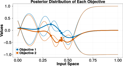
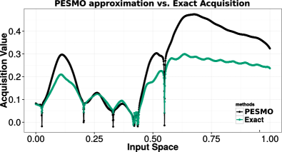
One question to be experimentally addressed is whether the proposed approximations are sufficiently accurate for effective identification of the Pareto set. We compare in a one-dimensional problem with two objectives the acquisition function computed by PESMO with a more accurate estimate obtained via expensive Monte Carlo sampling and a non-parametric estimator of the entropy Singh et al. (2003). Figure 1 (top) shows at a given step the observed data and the posterior mean and the standard deviation of each of the two objectives. The figure on the bottom shows the corresponding acquisition function computed by PESMO and by the Monte Carlo method (Exact). We observe that both functions look very similar, including the location of the global maximizer. This indicates that Eq. (7), obtained by expectation propagation, is potentially a good approximation of Eq. (2), the exact acquisition function. The supplementary material has extra results that show that each of the individual acquisition functions computed by PESMO, i.e., $\alpha_{k}(\cdot)$, for ${k=1,2}$, are also accurate.

Figure 1: (top) Observations of each objective and posterior mean and standard deviations of each GP model. (bottom) Estimates of the acquisition function (2) by PESMO, and by a Monte Carlo method combined with a non-parametric estimator of the entropy (Exact), which is expected to be more accurate. Best seen in color.

4.2 Experiments with Synthetic Objectives

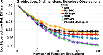
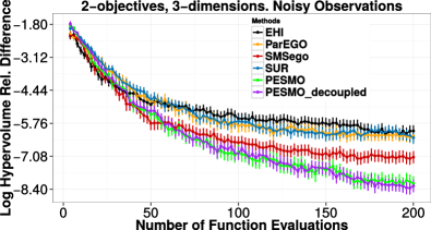
To initially compare PEMS with other approaches, we consider a 3-dimensional problem with 2 objectives obtained by sampling the functions from the corresponding GP prior. We generate 100 of these problems and report the average performance of each method, when considering noiseless observations and when the observations are contaminated with Gaussian noise with standard deviation equal to $0.1$. The performance metric employed is the hyper-volume indicator, which is maximized by the actual Pareto set Zitzler & Thiele (1999). More precisely, at each iteration we report the logarithm of the relative difference between the hyper-volume of the actual Pareto set, which is obtained by optimizing the actual objectives, and the hyper-volume of the recommendation, which is obtained by optimizing the posterior means of the GPs. Figure 2 (left-column) shows, as a function of the evaluations made, the average performance of each method with the corresponding error bars. PESMO obtains the best results, and when executed in a decoupled scenario slight improvements are observed, although only in the case of noisy observations.

Table 1 shows the average time in seconds required by each method to determine the next evaluation. The fastest method is ParEGO followed by SMSego and PESMO. The decoupled version of PESMO, $\text{{\small PESMO}}_{\text{dec}}$, takes more time because it has to optimize $\alpha_{1}(\cdot)$ and $\alpha_{2}(\cdot)$. The slowest methods are EHI and SUR; most of their cost is in the last iterations, in which the Pareto set size, $|\tilde{\mathcal{X}}^{\star}|$, is large due to non-dominated observations. The cost of evaluating the acquisition function in EHI and SUR is $\mathcal{O}((|\tilde{\mathcal{X}}^{\star}|+1)^{K})$, leading to expensive optimization via L-BFGS. In PESMO the cost of evaluating $\alpha(\cdot)$ is $\mathcal{O}(K|\mathcal{X}_{(s)}^{\star}|^{3})$ because $K$ linear systems are solved. These computations are faster because they are performed using the open-BLAS library, which is optimized for each processor. The acquisition function of EHI and SUR does not involve solving linear systems and hence these methods cannot use open-BLAS. Note that we also keep fixed $|\mathcal{X}_{(s)}^{\star}|=50$ in PESMO.

Figure 2: (left-column) Average log relative difference between the hyper-volume of the recommendation and the maximum hyper-volume for each number of evaluations made. We consider noiseless (top) and noisy observations (bottom). The problem considered has 2 objectives and 3 dimensions. (right-column) Similar results for a problem with 4 objectives and 6 dimensions. We do not compare results with EHI and SUR because they are infeasible due to their exponential cost with the number of objectives. Best seen in color.

Table 1: Avg. time in seconds doing calculations per iteration.

PESMO		$\text{PESMO}_{\text{dec}}$		ParEGO		SMSego		EHI		SUR
33$\pm$	1.0	52$\pm$	2.5	11$\pm$	0.2	16$\pm$	1.3	405$\pm$	115	623$\pm$	59

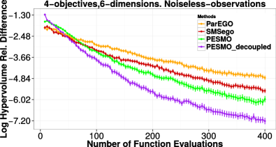
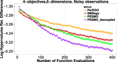
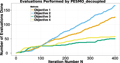
We have carried out additional synthetic experiments with 4 objectives on a 6-dimensional input space. In this case, EHI and SUR become infeasible, so we do not compare results with them. Again, we sample the objectives from the GP prior. Figure 2 (right-column) shows, as a function of the evaluations made, the average performance of each method. The best method is PESMO, and in this case, the decoupled evaluation performs significantly better. This improvement is because in the decoupled setting, PESMO identifies the most difficult objectives and evaluates them more times. In particular, because there are 4 objectives it is likely that some objectives are more difficult than others just by chance. Figure 3 illustrates this behavior for a representative case in which the first two objectives are non-linear (difficult) and the last two objectives are linear (easy). We note that the decoupled version of PESMO evaluates the first two objectives almost three times more.

Figure 3: (top) Contour curves of 4 illustrative objectives on 6 dimensions obtained by changing the first two dimensions in input space while keeping the other 4 fixed to zero. The first 2 objectives are non-linear while the 2 last objectives are linear. (bottom) Number of evaluations of each objective done by $\text{{\small PESMO}}_{\text{decoupled}}$ as a function of the iterations performed $N$. Best seen in color.

4.3 Finding a Fast and Accurate Neural Network

We consider the MNIST dataset (LeCun et al., 1998) and evaluate each method on the task of finding a neural network with low prediction error and small prediction time. These are conflicting objectives because reducing the prediction error will involve larger networks which will take longer at test time. We consider feed-forward networks with ReLus at the hidden layers and a soft-max output layer. The networks are coded in Keras (http://github.com/fchollet/keras) and they are trained using Adam (D. Kingma, 2014) with a minibatch size of $4,000$ instances during $150$ epochs. The adjustable parameters are: The number of hidden units per layer (between $50$ and $300$), the number of layers (between $1$ and $3$), the learning rate, the amount of dropout, and the level of $\ell_{1}$ and $\ell_{2}$ regularization. The prediction error is measured on a set of $10,000$ instances extracted from the training set. The rest of the training data, i.e., $50,000$ instances, is used for training. We consider a logit transformation of the prediction error because the error rates are very small. The prediction time is measured as the average time required for doing $10,000$ predictions. We compute the logarithm of the ratio between the prediction time of the network and the prediction time of the fastest network, (i.e., a single hidden layer and $50$ units). When measuring the prediction time we do not train the network and consider random weights (in Spearmint the time objective is also set to ignore irrelevant parameters). Thus, the problem is suited for a decoupled evaluation because both objectives can be evaluated separately. We run each method for a total of $200$ evaluations of the objectives and report results after $100$ and $200$ evaluations. Because there is no ground truth and the objectives are noisy, we re-evaluate 3 times the values associated with the recommendations made by each method (in the form of a Pareto set) and average the results. Then, we compute the Pareto front (i.e., the function space values of the Pareto set) and its hyper-volume. We repeat these experiments $50$ times and report the average results across repetitions.

Figure 4: Avg. Pareto fronts obtained by each method after 100 (left) and 200 (right) evaluations of the objectives. Best seen in color.

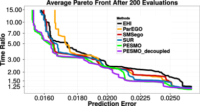Table 2 shows the hyper-volumes obtained in the experiments (the higher, the better). The best results, after $100$ evaluations of the objectives, correspond to the decoupled version of PESMO, followed by SUR and by the coupled version. When $200$ evaluations are done, the best method is PESMO in either setting, i.e., coupled or decoupled. After PESMO, SUR gives the best results, followed by SMSego and EHI. ParEGO is the worst performing method in either setting. In summary, PESMO gives the best overall results, and its decoupled version performs much better than the other methods when the number of evaluations is small.

Table 2: Avg. hyper-volume after $100$ and $200$ evaluations.

# Eval.	PESMO		$\text{PESMO}_{\text{dec}}$		ParEGO		SMSego		EHI		SUR
100	66.2$\pm$	.2	67.6$\pm$	.1	62.9$\pm$	1.2	65.0$\pm$	.3	64.0$\pm$	.9	66.6$\pm$	.2
200	67.8$\pm$	.1	67.8$\pm$	.1	66.1$\pm$	.2	67.1$\pm$	.2	66.6$\pm$	.2	67.2$\pm$	.1

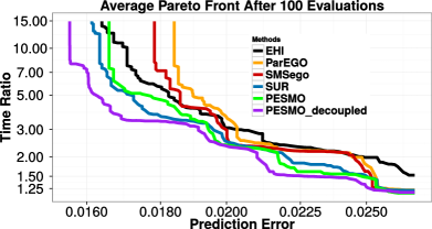
Figure 4 shows the average Pareto front obtained by each method after $100$ and $200$ evaluations of the objectives. The results displayed are consistent with the ones in Table 2. In particular, PESMO is able to find networks that are faster than the ones found by the other methods, for a similar prediction error on the validation set. This is especially the case of PESMO when executed in a decoupled setting, after doing only $100$ evaluations of the objectives. We also note that PESMO finds the most accurate networks, with almost $1.5\%$ of prediction error in the validation set.

Figure 5: Number of evaluations of each objective done by $\text{PESMO}_{\text{decoupled}}$, as a function of the iteration number $N$, in the problem of finding good neural networks. Best seen in color.

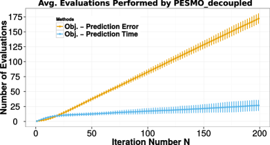
The good results obtained by $\text{{\small PESMO}}_{\text{decoupled}}$ are explained by Figure 5, which shows the average number of evaluations of each objective. More precisely, the objective that measures the prediction time is evaluated just a few times. This makes sense because it depends on only two parameters, i.e., the number of layers and the number of hidden units per layer. It is hence simpler than the prediction error. $\text{{\small PESMO}}_{\text{decoupled}}$ is able to detect this and focuses on the evaluation of the prediction error. Of course, evaluating the prediction error more times is more expensive, since it involves training the neural network more times. Nevertheless, this shows that $\text{{\small PESMO}}_{\text{decoupled}}$ is able to successfully discriminate between easy and difficult objective functions.

The supplementary material has extra experiments comparing each method on the task of finding an ensemble of decision trees of small size and good prediction accuracy.

5 Conclusions

We have described PESMO, a method for multi-objective Bayesian optimization. At each iteration, PESMO evaluates the objective functions at the input location that is most expected to reduce the entropy of posterior estimate of the Pareto set. Several synthetic experiments show that PESMO has better performance than other methods from the literature. That is, PESMO obtains better recommendations with a smaller number of evaluations, both in the case of noiseless and noisy observations. Furthermore, the acquisition function of PESMO can be understood as a sum of $K$ individual acquisition functions, one per each of the $K$ objectives. This allows for a decoupled evaluation scenario, in which the most promising objective is identified by maximizing the individual acquisition functions. When run in a decoupled evaluation setting, PESMO is able to identify the most difficult objectives and, by focusing on their evaluation, it provides better results. This behavior of PESMO has been illustrated on a multi-objective optimization problem that consists of finding an accurate and fast neural network. Finally, the computational cost of PESMO is small. In particular, it scales linearly with the number of objectives $K$. Other methods have an exponential cost with respect to $K$ which makes them infeasible for more than 3 objectives.

Appendix A Detailed Description of Expectation Propagation

In this section we describe in detail the specific steps of the EP algorithm that is required for the evaluation of the proposed acquisition function, PESMO. More precisely, we show how to compute the EP approximation to the conditional predictive distribution of each objective $f_{k}$. From the main manuscript we know that that this distribution is obtained by multiplying the GP posteriors by the product of all the approximate factors. We also show how to implement the EP updates to refine each approximate factor. In our implementation we assume independence among the $K$ objective functions.

We assume the reader is familiar with the steps of the expectation propagation algorithm, as described in Minka (2001b).

Recall from the main manuscript that all EP approximate factors $\tilde{\psi}$ are Gaussian and given by:

$$\tilde{\psi}(\mathbf{x}_{i},\mathbf{x}_{j}^{\star}) =\prod_{k=1}^{K}\tilde{\phi}_{k}(\mathbf{x}_{i},\mathbf{x}^{\star}_{j})\,,$$ (10)

where

$$\tilde{\phi}_{k}(\mathbf{x}_{i},\mathbf{x}_{j}^{\star}) =\exp\left\{-0.5\left(f_{k}(\mathbf{x}_{i})^{2}\tilde{v}_{i,j,k}+f_{k}(\mathbf{x}_{j}^{\star})^{2}\tilde{v}_{i,j,k}^{\star}+f_{k}(\mathbf{x}_{j}^{\star})f_{k}(\mathbf{x}_{i})\tilde{c}_{i,j,k}\right)\right.$$

$$\quad\left.+\tilde{m}_{i,j,k}f_{k}(\mathbf{x}_{i})+\tilde{m}_{i,j,k}^{\star}f_{k}(\mathbf{x}_{j}^{\star})\right\}\,,$$ (11)

for some input location $\mathbf{x}_{i}$ and for some $\mathbf{x}_{j}^{\star}$ extracted from the current sampled Pareto set $\mathcal{X}^{\star}$. Note that in (11), $\tilde{v}_{i,k}$, $\tilde{v}_{j,k}^{\star}$, $\tilde{c}_{i,j,k}$, $\tilde{m}_{i,k}$ and $\tilde{m}_{j,k}^{\star}$ are parameters fixed by EP.

A.1 Reconstruction of the Conditional Predictive Distribution

In this section we show how to obtain a conditional predictive distribution for each objective function $f_{k}$, given a sampled Pareto set $\mathcal{X}^{\star}=\{\mathbf{x}_{1}^{\star},\ldots,\mathbf{x}_{M}^{\star}\}$ of size $M$, and a set of $N$ input locations $\hat{\mathcal{X}}=\{\mathbf{x}_{1},\ldots,\mathbf{x}_{N}\}$, with corresponding observations of the $k$-th objective $\mathbf{y}_{k}$. We also assume that we are given the EP approximate factors $\tilde{\psi}$.

Define $\mathbf{f}_{k}=(f_{k}(\mathbf{x}_{1}^{\star}),\ldots,f_{k}(\mathbf{x}_{M}^{\star}),f_{k}(\mathbf{x}_{1}),\ldots,f_{k}(\mathbf{x}_{N}))^{\text{T}}$. We are interested in computing

$$p(\mathbf{f}_{k}|\mathcal{X}^{\star},\hat{\mathcal{X}},\mathbf{y}_{k}) \approx q(\mathbf{f}_{k})=Z^{-1}p(\mathbf{f}_{k}|\hat{\mathcal{X}},\mathbf{y}_{k})\prod_{\mathbf{x}\in\mathcal{X}^{\star}\cup\hat{\mathcal{X}}}\prod_{\begin{subarray}{c}\mathbf{x}^{\star}\neq\mathbf{x}\\ \mathbf{x}^{\star}\in\mathcal{X}^{\star}\end{subarray}}\tilde{\phi}_{k}(\mathbf{x},\mathbf{x}^{\star})\,,$$ (12)

for some normalization constant $Z$. In (12) we have only considered those approximate factors that depend on the current objective function $f_{k}$ and ignored the rest. We note that $p(\mathbf{f}_{k}|\hat{\mathcal{X}},\mathbf{y}_{k})$ is simply the posterior distribution of the Gaussian process, which is a multi-variate Gaussian over $N+M$ variables with natural parameters $\tilde{\bm{\Sigma}}^{k}$ and $\tilde{\bm{\mu}}^{k}$. Furthermore, all EP approximate factors $\tilde{\psi}$ are Gaussian. Because the Gaussian distribution is closed under the product operation, $q(\mathbf{f}_{k})$ is a multi-variate Gaussian distribution over $N+M$ variables with natural parameters $\mathbf{S}^{k}$ and $\mathbf{m}^{k}$ obtained as:

$$S_{i,i}^{k} =\tilde{\Sigma}_{i,i}^{k}+\sum_{j=M+1}^{N+M}\tilde{v}_{j,i,k}^{\star}+\sum_{j\neq i}\tilde{v}_{i,j,k}+\sum_{\begin{subarray}{c}j=1\\ j\neq i\end{subarray}}^{M}\tilde{v}_{j,i,k}^{\star}\quad\text{for}\quad i=1,\ldots,M\,,$$

$$S_{i,i}^{k} =\tilde{\Sigma}_{i,i}^{k}+\sum_{j=1}^{M}\tilde{v}_{i,j,k}\quad\text{for}\quad i=M+1,\ldots,N+M\,,$$

$$S_{i,j}^{k} =\tilde{\Sigma}_{i,j}^{k}+\tilde{c}_{i,j,k}\quad\text{for}\quad i=M+1,\ldots,N+M\,,\quad\text{and}\quad j=1,\ldots,M\,,$$

$$S_{i,j}^{k} =\tilde{\Sigma}_{j,i}^{k}+\tilde{c}_{j,i,k}+\tilde{c}_{i,j,k}\quad\text{for}\quad i=1,\ldots,M\,,\quad\text{and}\quad j=1,\ldots,M\,,\quad\text{and}\quad i\neq j\,,$$

$$S_{i,j}^{k} =\tilde{\Sigma}_{i,j}^{k}\quad\text{for}\quad i=M+1,\ldots,N+M\,,\quad\text{and}\quad j=M+1,\ldots,M+M\,,\quad\text{and}\quad i\neq j\,,$$

$$S_{j,i}^{k} =S_{i,j}^{k}\quad\text{for}\quad i\neq j\,,$$

$$m_{i}^{k} =\tilde{\mu}_{i}^{k}+\sum_{j=M+1}^{N+M}\tilde{m}_{j,i,k}^{\star}+\sum_{j\neq i}\tilde{m}_{i,j,k}+\sum_{\begin{subarray}{c}j=1\\ j\neq i\end{subarray}}^{M}\tilde{m}_{j,i,k}^{\star}\quad\text{for}\quad i=1,\ldots,M\,,$$

$$m_{i}^{k} =\tilde{\mu}_{i}^{k}+\sum_{j=1}^{M}\tilde{m}_{i,j,k}\quad\text{for}\quad i=M+1,\ldots,N+M\,.$$ (13)

From these natural parameters we can obtain, respectively, the covariance matrix $\bm{\Sigma}^{k}$ and the mean vector $\bm{\mu}^{k}$ by computing $(\mathbf{S}^{k})^{-1}$ and $(\mathbf{S}^{k})^{-1}\mathbf{m}^{k}$. This has a total cost that is $\mathcal{O}((N+M)^{3})$ since we have to invert a matrix of size $(N+M)\times(N+M)$. Importantly, this operations has to be performed only once at each iteration of the optimization process, and the result can be reused when evaluating the acquisition at different input locations.

A.2 The Conditional Predictive Distribution at a New Point

Consider now the computation of the conditional distribution for $f_{k}$ at a new candidate location $\mathbf{x}_{N+1}$. Assume that we have already obtained $q(\mathbf{f}_{k})$ from the previous section and that we have already obtained the parameters of the required approximate factors by using EP. We are interested in evaluating the conditional predictive variance for $f_{k}(\mathbf{x}_{N+1})$. For this, we need to evaluate:

$$p(f_{k}(\mathbf{x}_{N+1})|\hat{\mathcal{X}},\mathcal{X}^{\star},\mathbf{x}_{N+1}) \approx\int{Z}^{-1}q(\mathbf{f}_{k},f_{k}(\mathbf{x}_{N+1}))\prod_{\mathbf{x}^{\star}\in\mathcal{X}^{\star}}\tilde{\phi}_{k}(\mathbf{x}_{N+1},\mathbf{x}^{\star})d\mathbf{f}_{k}\,,$$ (14)

where $Z$ is simply a normalization constant and $q(\mathbf{f}_{k},f_{k}(\mathbf{x}_{N+1}))$ is a multivariate Gaussian distribution which results by extending $q(\mathbf{f}_{k})$ with one extra dimension for $f_{k}(\mathbf{x}_{N+1})$. Recall that $\mathbf{f}_{k}=(f_{k}(\mathbf{x}_{1}^{\star}),\allowbreak\ldots,f_{k}(\mathbf{x}_{M}^{\star}),f_{k}(\mathbf{x}_{1}),\ldots,f_{k}(\mathbf{x}_{N}))^{\text{T}}$. Again, in (14) we have only considered those approximate factors that depend on $f_{k}$. The covariances between $\mathbf{f}_{k}$ and $f_{k}(\mathbf{x}_{N+1})$ are obtained from the GP posterior for $f_{k}$ given the observed data. The mean and the variance of $f_{k}(\mathbf{x}_{N+1})$ to be used in $q(\mathbf{f}_{k},f_{k}(\mathbf{x}_{N+1}))$ can also be obtained in a similar way. Because all the factors in the r.h.s. of (14) are Gaussian, the result of the integral is a univariate Gaussian distribution.

Define $\tilde{\mathbf{f}}_{k}=(f_{k}(\mathbf{x}_{1}^{\star}),\ldots,f_{k}(\mathbf{x}_{M}^{\star}),f_{k}(\mathbf{x}_{N+1}))^{\text{T}}$. Because $\prod_{\mathbf{x}^{\star}\in\mathcal{X}^{\star}}\tilde{\phi}_{k}(\mathbf{x}_{N+1},\mathbf{x}^{\star})$ does not depend on $f_{k}(\mathbf{x}_{1}),\ldots,f_{k}(\mathbf{x}_{N})$, we can marginalize these variables in the r.h.s. of (14) to get something proportional to:

$$\int q(\tilde{\mathbf{f}}_{k})\prod_{\mathbf{x}^{\star}\in\mathcal{X}^{\star}}\tilde{\phi}_{k}(\mathbf{x}_{N+1},\mathbf{x}^{\star})\prod_{i=1}^{M}df_{k}(\mathbf{x}_{i}^{\star})\propto\int\mathcal{N}(\tilde{\mathbf{f}}_{k}|(\mathbf{S}^{x})^{-1}\mathbf{m}^{x},(\mathbf{S}^{x})^{-1})\prod_{i=1}^{M}df_{k}(\mathbf{x}_{i}^{\star})=$$

$$\mathcal{N}(f_{k}(\mathbf{x}_{N+1})|m_{x},\sigma_{x}^{2})\,,$$ (15)

where $\mathbf{m}^{x}$ and $\mathbf{S}^{x}$ are the natural parameters of the approximate conditional predictive distribution for $\tilde{\mathbf{f}}_{k}$, which is Gaussian. Similarly, $m_{x}$ and $\sigma_{x}^{2}$ are the mean and variance of the Gaussian approximation to $p(f_{k}(\mathbf{x}_{N+1}|\hat{\mathcal{X}},\mathcal{X}^{\star},\mathbf{x}_{N+1})$.

We are interested in the evaluation of $\sigma_{x}^{2}$, which is required for entropy computation. It is clear that $\sigma_{x}^{2}$ is given by the last diagonal entry of $(\mathbf{S}^{x})^{-1}$. In consequence, we now show how to compute $\mathbf{S}^{x}$ and $(\mathbf{S}^{x})^{-1}_{M+1,M+1}$. We do not give the details for computing $m_{x}$, because only the variance is required for the entropy computation.

Each entry in $\mathbf{S}^{x}$ is given by:

$$S_{i,j}^{x} =S_{i,j}^{k}\quad\text{for}\quad 1\leq i\leq M\quad\text{and}\quad 1\leq j\leq M\,,\quad\text{and}\quad i\neq j\,,$$

$$S_{i,j}^{x} =\text{cov}(f_{k}(\mathbf{x}_{N+1}),f(\mathbf{x}_{j}^{\star}))+\tilde{c}_{N+1,j,k}\quad\text{for}\quad 1\leq j\leq M\quad\text{and}\quad i=M+1\,,$$

$$S_{j,i}^{x} =S_{i,j}^{x}\quad\text{for}\quad j\neq i\,,\quad\text{and}\quad 1\leq i,j\leq M\,,$$

$$S_{i,i}^{x} =S_{i,i}^{k}+\tilde{v}_{N+1,j,k}^{\star}\,,\text{for}\quad 1\leq i\leq M\,,$$

$$S_{M+1,M+1}^{x} =\text{var}(f_{k}(\mathbf{x}_{N+1}))+\sum_{j=1}^{M}\tilde{v}_{N+1,j,k}\,,$$ (16)

where $\tilde{v}_{N+1,i,k}$, $\tilde{v}_{N+1,i,k}^{\star}$, and $\tilde{c}_{N+1,i,k}$ are the parameters of each of the $M$ factors $\tilde{\phi}_{k}(\mathbf{x}_{N+1},\mathbf{x}_{j}^{\star})$, for $j=1,\ldots,M$. Furthermore, $\text{var}(f_{k}(\mathbf{x}_{N+1}))$ and $\text{cov}(f_{k}(\mathbf{x}_{N+1})$ are the posterior variance of $f_{k}(\mathbf{x}_{N+1})$ and the posterior covariance between $f_{k}(\mathbf{x}_{N+1})$ and $f_{k}(\mathbf{x}_{j}^{\star})$.

We note that $\mathbf{S}^{x}$ has a block structure in which only the last row and column depend on $\mathbf{x}_{N+1}$. This allows to compute $\sigma_{x}^{2}=(\mathbf{S}^{x})^{-1}_{M+1,M+1}$ with cost $\mathcal{O}(M^{3})$ using the formulas for block matrix inversion. All these computations are carried out using the open-BLAS library for linear algebra operations which is particularly optimized for each processor.

Given $\sigma_{x}^{2}$ we only have to add the variance of the additive Gaussian noise $\epsilon^{k}_{N+1}$ to obtain the final variance of the Gaussian approximation to the conditional predictive distribution of $y^{k}_{N+1}=f_{k}(\mathbf{x}_{N+1})+\epsilon_{N+1}^{k}$.

A.3 Update of an Approximate Factor

EP updates until convergence each of the approximate factors $\tilde{\psi}$. Given an exact factor $\psi(\mathbf{x}_{i},\mathbf{x}_{j}^{\star})$, in this section we show how to update the corresponding EP approximate factor $\tilde{\psi}(\mathbf{x}_{i},\mathbf{x}_{j}^{\star})$. For this, we assume that we have already obtained the parameters $\bm{\mu}^{k}$ and $\bm{\Sigma}^{k}$ of each of the $K$ conditional predictive distributions, $q(\mathbf{f}_{k})$, as described in Section A.1. The form of the exact factor is:

$$\psi(\mathbf{x}_{i},\mathbf{x}_{j}^{\star}) =1-\prod_{k=1}^{K}\Theta\left(f_{k}(\mathbf{x}_{j}^{\star})-f_{k}(\mathbf{x}_{i})\right)\,.$$ (17)

Note that this factor only depends on $f_{k}(\mathbf{x}_{i})$ and $f_{k}(\mathbf{x}_{j}^{\star})$ for $k=1,\ldots,K$. This means that we are only interested in the distribution of these variables under $q(\mathbf{f}_{k})$, for $k=1,\ldots,K$, and can ignore (marginalize in $q$) all other variables. Thus, in practice we will work with $q(f_{k}(\mathbf{x}_{i}),f_{k}(\mathbf{x}_{j}^{\star}))$, for $k=1,\ldots,K$. These are bi-variate Gaussian distributions. Let the means, variances and covariance parameters of one of these distributions be respectively: $m_{i,j,k}$, $m_{i,j,k}^{\star}$, $v_{i,j,k}$, $v_{i,j,k}^{\star}$ and $c_{i,j,k}$.

A.3.1 Computation of the Cavity Distribution

The first step of the update is to compute and old distribution $q^{\text{old}}$, known as the cavity distribution, which is obtained by removing the approximate factor $\tilde{\psi}(\mathbf{x}_{i},\mathbf{x}_{j}^{\star})$ from the product of the $K$ approximations $q(f_{k}(\mathbf{x}_{i}),f_{k}(\mathbf{x}_{j}^{\star}))$, for $k=1,\ldots,K$. Recall that $\tilde{\psi}(\mathbf{x}_{i},\mathbf{x}_{j}^{\star})=\prod_{k=1}^{K}\tilde{\phi}_{k}(\mathbf{x}_{i},\mathbf{x}_{j}^{\star})$. This can be done by division. Namely, $q^{\text{old}}(f_{k}(\mathbf{x}_{i}),f_{k}(\mathbf{x}_{j}^{\star}))\propto q(f_{k}(\mathbf{x}_{i}),f_{k}(\mathbf{x}_{j}^{\star}))/\tilde{\phi}_{k}(\mathbf{x}_{i},\mathbf{x}_{j}^{\star})$, for $k=1,\ldots,K$. Because all the factors are Gaussian, the result is another bi-variancete Gaussian distribution. Let the corresponding old parameters be: $m^{\text{old}}_{i,j,k}$, $m^{\text{old}\star}_{i,j,k}$, $v^{\text{old}}_{i,j,k}$, $v_{i,j,k}^{\text{old}\star}$ and $c^{\text{old}}_{i,j,k}$. These parameters are obtained by subtracting from the natural parameters of $q(f_{k}(\mathbf{x}_{i}),f_{k}(\mathbf{x}_{j}^{\star}))$, the natural parameters of $\tilde{\phi}_{k}$. The resulting natural parameters are then transformed into standard mean and covariance parameters to get the parameters of $q^{\text{old}}(f_{k}(\mathbf{x}_{i}),f_{k}(\mathbf{x}_{j}^{\star}))$. This step is performed as indicated in the last paragraph of Section A.1, and it involves computing the inverse of a $2\times 2$ matrix, which is something very easy and inexpensive to do in practice.

A.3.2 Computation of the Moments of the Tilted Distribution

Given each $q^{\text{old}}(f_{k}(\mathbf{x}_{i}),f_{k}(\mathbf{x}_{j}^{\star}))$, for $k=1,\ldots,K$, the next step of the EP algorithm is to compute the moments of a tilted distribution defined as:

$$\hat{p}(\{f_{k}(\mathbf{x}_{i}),f_{k}(\mathbf{x}_{j}^{\star})\}_{k=1}^{K}) =\hat{Z}^{-1}\psi(\mathbf{x}_{i},\mathbf{x}_{j}^{\star})\prod_{k=1}^{K}q^{\text{old}}(f_{k}(\mathbf{x}_{i}),f_{k}(\mathbf{x}_{j}^{\star}))\,,$$ (18)

where $\hat{Z}$ is just a normalization constant that guarantees that $\hat{p}$ integrates up to one.

Importantly, the normalization constant $\hat{Z}$ can be computed in closed form and is given by:

$$\hat{Z} =1-\prod_{k=1}^{K}\Phi\left(\frac{m^{\text{old}}_{i,j,k}-m^{\text{old}\star}_{i,j,k}}{\sqrt{v^{\text{old}}_{i,j,k}+v^{\text{old}\star}_{i,j,k}-2c^{\text{old}}_{i,j,k}}}\right)\,,$$ (19)

where $\Phi(\cdot)$ is the c.p.f. of a standard Gaussian distribution. The moments (mean vector and covariance matrix) of $\hat{p}$ can be readily obtained from the derivatives of $\log\hat{Z}$ with respect to the parameters of $q^{\text{old}}(f_{k}(\mathbf{x}_{i}),f_{k}(\mathbf{x}_{j}^{\star}))$, as indicated in the Appendix of Hernández-Lobato (2009).

A.3.3 Computation of the Individual Approximate Factors

Given the moments of the tilted distribution $\hat{p}(\{f_{k}(\mathbf{x}_{i}),f_{k}(\mathbf{x}_{j}^{\star})\}_{k=1}^{K})$, it is straight-forward to obtain the parameters of the approximate factors $\tilde{\phi}_{k}$, for $k=1,\ldots,K$, whose product approximates $\psi(\mathbf{x}_{i},\mathbf{x}_{j}^{\star})$. The idea is that the product of $\tilde{\psi}(\mathbf{x}_{i},\mathbf{x}_{j}^{\star})=\prod_{i=1}^{K}\tilde{\phi}_{k}(\mathbf{x}_{i},\mathbf{x}_{j}^{\star})$ and $\prod_{k=1}^{K}q^{\text{old}}(f_{k}(\mathbf{x}_{i}),f_{k}(\mathbf{x}_{j}^{\star}))$ should lead to a Gaussian distribution with the same moments as the tilted distribution $\hat{p}$.

The detailed steps to find each $\tilde{\phi}_{k}$ are: (i) Define a Gaussian distribution with the same moments as $\hat{p}$, denoted $\prod_{k=1}^{K}q^{\text{new}}(f_{k}(\mathbf{x}_{i}),f_{k}(\mathbf{x}_{j}^{\star}))$. Note that this distribution factorizes across each objective $k$. Let the parameters of this distribution be $m^{\text{new}}_{i,j,k}$, $m^{\text{new}\star}_{i,j,k}$, $v^{\text{new}}_{i,j,k}$, $v_{i,j,k}^{\text{new}\star}$ and $c^{\text{new}}_{i,j,k}$, for $k=1,\ldots,K$. (ii) Transform these parameters to natural parameters, and subtract to them the natural parameters of $\prod_{k=1}^{K}q^{\text{old}}(f_{k}(\mathbf{x}_{i}),f_{k}(\mathbf{x}_{j}^{\star}))$. (iii) The resulting natural parameters are the natural parameters of each updated $\tilde{\phi}_{k}$. Note that this operation involves going from standard parameters to natural parameters. Again, this can be done as indicated in the last paragraph of Section A.1. For this, the inverse of the corresponding $2\times 2$ covariance matrix of each Gaussian factor of $\prod_{k=1}^{K}q^{\text{new}}(f_{k}(\mathbf{x}_{i}),f_{k}(\mathbf{x}_{j}^{\star}))$ is required. Because these are $2\times 2$ matrices, this operation is inexpensive and very fast to compute.

A.4 Parallel EP Updates and Damping

In our EP implementation we updated in parallel each of the approximate factors $\tilde{\psi}$, as indicated in Gerven et al. (2009). That is, we computed the corresponding cavity distribution for each factor $\psi$ and updated the corresponding approximate factor $\tilde{\psi}$ afterwards. Next, the EP approximation was reconstructed as indicated in Section A.1.

We also employed damped EP updates in our implementation Minka & Lafferty (2002). That is, the parameters of each updated factor are set to be a linear combination of the old parameters and the new parameters. The use of damped updates prevents very large changes in the parameter values. It is hence very useful to improve the convergence properties of the algorithm. Finally, damping does not change the convergence points of EP.

Appendix B Finding a Small and Accurate Ensemble of Decision Trees

In this section we evaluate each of the methods from the main manuscript in the task of finding an ensemble of decision trees of small size that has low prediction error. We measure the ensemble size in terms of the sum of the total number of nodes in each of trees of the ensemble. Note that the objectives considered are conflicting because it is expected that an ensemble of small size has higher prediction error than an ensemble of larger size. The dataset considered is the German Credit dataset, which is extracted from the UCI repository Lichman (2013). This is a binary classification dataset with 1,000 instances and 9 attributes. The prediction error is measured using a 10-fold-cross validation procedure that is repeated 5 times to reduce the variance of the estimates.

Critically, to get ensembles of decision trees with good prediction properties one must encourage diversity in the ensemble Dietterich (2000). In particular, if all the decision trees are equal, there is no gain from aggregating them in an ensemble. However, too much diversity can also lead to ensembles of poor prediction performance. For example, if the predictions made are completely random, one cannot obtain improved results by aggregating the individual classifiers. In consequence, we consider here several mechanisms to encourage diversity in the ensemble, and let the amount of diversity be specified in terms of adjustable parameters.

To build the ensemble we employed decision trees in which the data is split at each node, and the best split is chosen by considering each time a random set of attributes —we use the Decision-Tree implementation provided in the python package scikit-learn for this, and the number of random attributes is an adjustable parameter. This is the approach followed in Random Forest Breiman (2001) to generate the ensemble classifiers. Each tree is trained on a random subset of the training data of a particular size, which is another adjustable parameter. This approach is known in the literature as subbagging Bühlmann & Yu (2001), and has been shown to lead to classification ensembles with good prediction properties. We consider also an extra method to introduce diversity known as class-switching Martínez-Muñoz & Suárez (2005). In class-switching, the labels of a random fraction of the training data are changed to a different class. The final ensemble prediction is computed by majority voting.

In summary, the adjustable parameters are: the number of decision trees built (between $1$ and $1,000$), the number of random features considered at each split in the building process of each tree (between $1$ and $9$), the minimum number of samples required to split a node (between $2$ and $200$), the fraction of randomly selected training data used to build each tree, and the fraction of training instances whose labels are changed (after doing the sub-sampling process).

Finally, we note that this setting is suited to the decoupled version of PESMO since both objectives can be evaluated separately. In particular, the total number of nodes is estimated by building only once the ensemble without leaving any data aside for validation, as opposed to the cross-validation approach used to estimate the ensemble error, which requires to build several ensembles on subsets of the data, to then estimate the prediction error on the data left out for validation.

We run each method for $200$ evaluations of the objectives and report results after $100$ and $200$ evaluations. That is, after $100$ and $200$ evaluations, we optimize the posterior means of the GPs and provide a recommendation in the form of a Pareto set. As in the experiments reported in the main manuscript with neural networks, we re-estimate three times the objectives associated to each Pareto point from the recommendation made by each method, and average results. The goal of this averaging process is to reduce the noise in the final evaluation of the objectives. These final evaluations are used to estimate the performance of each method using the hyper-volume. We repeat these experiments $50$ times and report the average results across repetitions.

Table 3: Avg. hyper-volume after $100$ and $200$ evaluations of the objectives.

# Eval.	PESMO		$\text{PESMO}_{\text{dec}}$		ParEGO		SMSego		EHI		SUR
100	8.742$\pm$	.006	8.755$\pm$	.009	8.662$\pm$	.019	8.719$\pm$	.012	8.731$\pm$	.009	8.739$\pm$	.007
200	8.764$\pm$	.007	8.758$\pm$	.007	8.705$\pm$	.008	8.742$\pm$	.006	8.727$\pm$	.008	8.756$\pm$	.006

Table 3 shows the average hyper-volume of the recommendations made by each method, after 100 and 200 evaluations of the objective functions. The table also shows the corresponding error bars. In this case the observed differences among the different methods are smaller than in the experiments with neural networks. Nevertheless, we observe that the decoupled version of PESMO obtains the best results after 100 evaluations. After this, PESMO in the coupled setting performs best, closely followed by SUR. After 200 evaluations, the best method is the coupled version of PESMO, closely followed by its decoupled version and by SUR. SMSego and EHI give worse results than these methods, in general. Finally, as in the experiments with neural networks reported in the main manuscript, ParEGO is the worst performing method. In summary, the best methods are PESMO in either setting (coupled or decoupled) and SUR. All other methods perform worse. Furthermore, the decoupled version of PESMO gives slightly better results at the beginning, i.e., after 100 evaluations.

Figure 6: Avg. Pareto fronts obtained by each method after 100 (top) and 200 (bottom) evaluations of the objectives. Best seen in color.

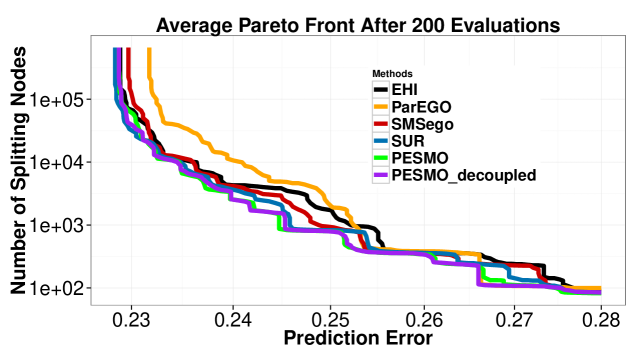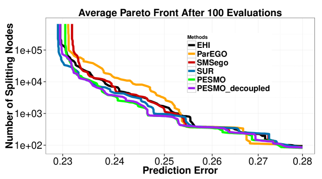
Figure 6 shows the average Pareto front (this is simply the values in functional space associated to the Pareto set) corresponding to the recommendations made by each method after 100 (top) and 200 evaluations of the objectives (bottom). We observe that PESMO finds ensembles with better properties than the ones found by EHI, SMSego and ParEGO. Namely, ensembles of smaller size for a similar or even better prediction error. The most accurate ensembles are found by SUR. Nevertheless, they have a very similar error to the one of the most accurate ensembles found by PESMO. Finally, we note that in some cases, PESMO is able to find ensembles of intermediate size with better prediction error than the ones found by SUR.

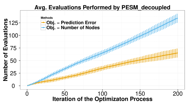
Figure 7 shows the average number of times that the decoupled version of PESMO evaluates each objective. We observe that in this case the objective that measures the number of nodes in the ensemble is evaluated more times. However, the difference between the number of evaluations of each objective is smaller than the difference observed in the case of the experiments with neural networks. Namely, 135 evaluations of one objective versus 65 evaluations of the other, in this case, compared to 175 evaluations versus 25 evaluations, in the case of the experiments with neural networks. This may explain why in this case the differences between the coupled and the decoupled version of PESMO are not as big as in the experiments reported in the main manuscript.

Figure 7: Number of evaluations of each objective done by $\text{PESMO}_{\text{decoupled}}$, as a function of the iteration number $N$, in the problem of finding a good ensemble of decision trees. Best seen in color.

Appendix C Accuracy of the Acquisition in the Decoupled Setting

One question to be experimentally addressed is whether the proposed approximations for the individual acquisition functions $\alpha_{k}(\cdot)$, for $k=1,\ldots,K$, with $K$ the total number of objectives are sufficiently accurate in the decoupled case of PESMO. For this, we extend the experiment carried out in the main manuscript, and compare in a one-dimensional problem with two objectives the acquisition functions $\alpha_{1}(\cdot)$ and $\alpha_{2}(\cdot)$ computed by PESMO, with a more accurate estimate obtained via expensive Monte Carlo sampling and a non-parametric estimator of the entropy Singh et al. (2003). This estimate measures the expected decrease in the entropy of the predictive distribution of one of the objectives, at a given location of the input space, after conditioning to the Pareto set. Importantly, in the decoupled case, the observations corresponding to each objective need not be located at the same input locations.

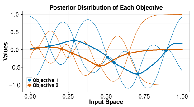
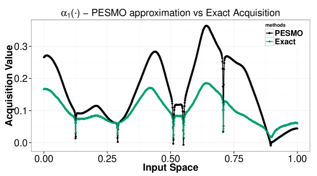
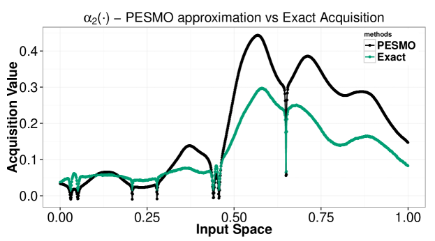
Figure 8 (top) shows at a given step of the optimization process, the observed data and the posterior mean and the standard deviation of each of the two objectives. The figure on the middle shows the corresponding acquisition function corresponding to the first objective, $\alpha_{1}(\cdot)$, computed by PESMO and by the Monte Carlo method (Exact). The figure on the bottom shows the same results for the acquisition function corresponding to the second objective, $\alpha_{2}(\cdot)$. We observe that both functions look very similar, including the location of the global maximizer. This indicates that the approximation obtained by expectation propagation is potentially good also in the decoupled setting.

Figure 8: (top) Observations of each objective and posterior mean and standard deviations of each GP model. (middle) Estimates of the acquisition function corresponding to the first objective, $\alpha_{1}(\dot{)}$, by PESMO, and by a Monte Carlo method combined with a non-parametric estimator of the entropy. (bottom) Same results for the acquisition function corresponding to the second objective $\alpha_{2}(\cdot)$. Best seen in color.

References

- Ariizumi et al. (2014) Ariizumi, R., Tesch, M., Choset, H., and Matsuno, F. Expensive multiobjective optimization for robotics with consideration of heteroscedastic noise. In 2014 IEEE International Conference on Intelligent Robots and Systems, pp. 2230–2235, 2014.
- Breiman (2001) Breiman, Leo. Random forests. Machine Learning, 45:5–32, 2001.
- Bühlmann & Yu (2001) Bühlmann, Peter and Yu, Bin. Analyzing Bagging. Annals of Statistics, 30:927–961, 2001.
- Collette & Siarry (2003) Collette, Y. and Siarry, P. Multiobjective Optimization: Principles and Case Studies. Springer, 2003.
- D. Kingma (2014) D. Kingma, J. Ba. Adam: A method for stochastic optimization. 2014. arXiv:1412.6980.
- Deb et al. (2002) Deb, K., Pratap, A., Agarwal, S., and Meyarivan, T. A fast and elitist multiobjective genetic algorithm: NSGA-II. IEEE Transactions on Evolutionary Computation, 6:182–197, 2002.
- Dietterich (2000) Dietterich, Thomas G. Ensemble methods in machine learning. In Multiple classifier systems, pp. 1–15. Springer, 2000.
- Emmerich (2008) Emmerich, A. The computation of the expected improvement in dominated hypervolume of Pareto front approximations. Technical Report LIACS TR-4-2008, Leiden University, The Netherlands, 2008.
- Gelbart et al. (2014) Gelbart, Michael A., Snoek, Jasper, and Adams, Ryan P. Bayesian optimization with unknown constraints. In Thirtieth Conference on Uncertainty in Artificial Intelligence, 2014.
- Gerven et al. (2009) Gerven, Marcel Van, Cseke, Botond, Oostenveld, Robert, and Heskes, Tom. Bayesian source localization with the multivariate Laplace prior. In Advances in Neural Information Processing Systems 22, pp. 1901–1909, 2009.
- Henning & Schuler (2012) Henning, P. and Schuler, C. J. Entropy search for information-efficient global optimization. Journal of Machine Learning Research, 13:1809–1837, 2012.
-
Hernández-Lobato (2009)
Hernández-Lobato, Daniel.
Prediction Based on Averages over Automatically Induced
Learners: Ensemble Methods and Bayesian Techniques.
PhD thesis, Computer Science Department, Universidad Autónoma
de Madrid, 2009.
Online available at: http://arantxa.ii.uam.es/d̃hernan/
docs/Thesis_color_links.pdf. - Hernández-Lobato et al. (2014) Hernández-Lobato, J. M., Hoffman, M. W., and Ghahramani, Z. Predictive entropy search for efficient global optimization of black-box functions. In Advances in Neural Information Processing Systems 27, pp. 918–926. 2014.
- Houlsby et al. (2012) Houlsby, N., Hernández-lobato, J. M., H., F., and Ghahramani, Z. Collaborative gaussian processes for preference learning. In Advances in Neural Information Processing Systems 25, pp. 2096–2104. 2012.
- Hupkens et al. (2014) Hupkens, I., Emmerich, M., and Deutz, A. Faster computation of expected hypervolume improvement. 2014. arXiv:1408.7114 [cs.DS].
- Jones et al. (1998) Jones, D. R., Schonlau, M., and Welch, W. J. Efficient global optimization of expensive black-box functions. Journal of Global Optimization, 13(4):455–492, 1998.
- Knowles (2006) Knowles, J. ParEGO: a hybrid algorithm with on-line landscape approximation for expensive multiobjective optimization problems. IEEE Transactions on Evolutionary Computation, 10:50–66, 2006.
- LeCun et al. (1998) LeCun, Y., Bottou, L., Bengio, Y., and Haffner, P. Gradient-based learning applied to document recognition. Proceedings of the IEEE, 86(11):2278–2324, 1998.
- Li (2003) Li, X. A non-dominated sorting particle swarm optimizer for multiobjective optimization. In Genetic and Evolutionary Computation — GECCO 2003, pp. 37–48. 2003.
- Lichman (2013) Lichman, M. UCI machine learning repository, 2013. URL http://archive.ics.uci.edu/ml.
- Martínez-Muñoz & Suárez (2005) Martínez-Muñoz, Gonzalo and Suárez, Alberto. Switching class labels to generate classification ensembles. Pattern Recognition, 38:1483–1494, 2005.
- Minka (2001a) Minka, T. A Family of Algorithms for Approximate Bayesian Inference. PhD thesis, MIT, 2001a.
- Minka (2001b) Minka, T. Expectation propagation for approximate Bayesian inference. In Annual Conference on Uncertainty in Artificial Intelligence, pp. 362–36, 2001b.
- Minka & Lafferty (2002) Minka, T. and Lafferty, J. Expectation-propagation for the generative aspect model. In Proceedings of the 18th Conference on Uncertainty in Artificial Intelligence, pp. 352–359, 2002.
- Mockus et al. (1978) Mockus, J., Tiesis, V., and Zilinskas, A. The application of Bayesian methods for seeking the extremum. Towards Global Optimization, 2(117-129):2, 1978.
- Nakayama et al. (2009) Nakayama, H., Yun, Y., and M.Yoon. Sequential Approximate Multiobjective Optimization Using Computational Intelligence. Springer, 2009.
- Picheny (2015) Picheny, V. Multiobjective optimization using Gaussian process emulators via stepwise uncertainty reduction. Statistics and Computing, 25:1265–1280, 2015.
- Ponweiser et al. (2008) Ponweiser, W., Wagner, T., Biermann, D., and Vincze, M. Multiobjective optimization on a limited budget of evaluations using model-assisted -metric selection. In Parallel Problem Solving from Nature – PPSN X, pp. 784–794. 2008.
- Rasmussen & Williams (2006) Rasmussen, C. E. and Williams, C. K. I. Gaussian Processes for Machine Learning (Adaptive Computation and Machine Learning). The MIT Press, 2006.
- Shah & Ghahramani (2015) Shah, A. and Ghahramani, Z. Parallel predictive entropy search for batch global optimization of expensive objective functions. In Advances in Neural Information Processing Systems 28, pp. 3312–3320. 2015.
- Singh et al. (2003) Singh, H., Misra, N., Hnizdo, V., Fedorowicz, A., and Demchuk, E. Nearest neighbor estimates of entropy. American journal of mathematical and management sciences, 23:301–321, 2003.
- Villemonteix et al. (2009) Villemonteix, J., Vazquez, E., and Walter, E. An informational approach to the global optimization of expensive-to-evaluate functions. Journal of Global Optimization, 44:509–534, 2009.
- Zitzler & Thiele (1999) Zitzler, E. and Thiele, L. Multiobjective evolutionary algorithms: a comparative case study and the strength pareto approach. IEEE Transactions on Evolutionary Computation, 3:257–271, 1999.
- Zuluaga et al. (2013) Zuluaga, M., Krause, A., Sergent, G., and Püschel, M. Active learning for multi-objective optimization. In International Conference on Machine Learning, pp. 462–470, 2013.