Quantile universal threshold for model selection
Efficient recovery of a low-dimensional structure from high-dimensional data has been pursued in various settings including wavelet denoising, generalized linear models and low-rank matrix estimation. By thresholding some parameters to zero, estimators such as lasso, elastic net and subset selection allow to perform not only parameter estimation but also variable selection, leading to sparsity. Yet one crucial step challenges all these estimators: the choice of the threshold parameter . If too large, important features are missing; if too small, incorrect features are included.
Within a unified framework, we propose a new selection of at the detection edge under the null model. To that aim, we introduce the concept of a zero-thresholding function and a null-thresholding statistic, that we explicitly derive for a large class of estimators. The new approach has the great advantage of transforming the selection of from an unknown scale to a probabilistic scale with the simple selection of a probability level. Numerical results show the effectiveness of our approach in terms of model selection and prediction.
Keywords: Convex optimization, high-dimensionality, sparsity, regularization, thresholding, variable screening.
1 Introduction
Many real world examples in which the number of features of the model can be dramatically larger than the sample size have been identified in various domains such as genomics, finance and image classification, to name a few. In those instances, the maximum likelihood estimation principle fails. Beyond existence and uniqueness issues, it tends to perform poorly when is large relative to due to its high variance. Motivated by the seminal papers of James and Stein (1961) and Tikhonov (1963), a considerable amount of literature has concentrated on parameter estimation using regularization techniques. In both parametric and nonparametric models, a reasonable prior or constraints are set on the parameters in order to reduce the variance of the estimator and the complexity of the fitted model, at the price of a bias increase.
We consider a class of regularization techniques, called thresholding, which:
-
(i)
assumes a certain transform of the true model parameter is sparse, meaning
(1) has small cardinality. For example, coordinate-sparsity is induced by , whereas variation-sparsity is induced by with the first order difference matrix;
-
(ii)
results in an estimated support
(2) whose cardinality is governed by the choice of a threshold parameter .
Thresholding techniques are employed in various settings such as linear regression (Donoho and Johnstone, 1994; Tibshirani, 1996), generalized linear models (Park and Hastie, 2007), low-rank matrix estimation (Mazumder et al., 2010; Cai et al., 2010), density estimation (Donoho et al., 1996; Sardy and Tseng, 2010), linear inverse problems (Donoho, 1995), compressed sensing (Donoho, 2006; Candès and Romberg, 2007) and time series (Neto et al., 2012).
Selection of the threshold is crucial to perform effective model selection. It amounts to selecting basis coefficients in wavelet denoising, or genes responsible for a cancer type in microarray data analysis. In change-point detection, it is equivalent to detecting locations of jumps of a function. A too large results in a simplistic model missing important features whereas a too small leads to a model including many features outside the true model. A typical goal is variable screening, that is,
| (3) |
holds with high probability, along with few false detections . For a suitably chosen , certain estimators allow variable screening. The optimal threshold for model identification often differs from the threshold aimed at prediction optimality (Yang, 2005; Leng et al., 2006; Meinshausen and Bühlmann, 2006; Zou, 2006), and it turns out that models aimed at good prediction are typically more complex.
Classical methodologies to select consist in minimizing a criterion. Examples include cross-validation, AIC (Akaike, 1998), BIC (Schwarz, 1978) and Stein unbiased risk estimation (SURE) (Stein, 1981). In low-rank matrix estimation, Owen and Perry (2009) and Josse and Husson (2012) employ cross-validation whereas Candès et al. (2013) and Josse and Sardy (2016) apply SURE. The latter methodology is also used in regression (Donoho and Johnstone, 1994; Zou et al., 2007; Tibshirani and Taylor, 2012), and reduced rank regression (Mukherjee et al., 2015). Because traditional information criteria do not adapt well to the high-dimensional setting, generalizations such as GIC (Fan and Tang, 2013) and EBIC (Chen and Chen, 2008) have been suggested.
In this paper, we propose a new threshold selection method that aims at a good identification of the support , and that follows the same paradigm in various domains. Our approach has the advantage of transforming the selection of from an unknown scale to a probabilistic scale with the simple selection of a probability level. In Section 2, we first review thresholding estimators in linear regression, generalized linear models, low-rank matrix estimation and density estimation. We then introduce the key concept of a zero-thresholding function in Section 3 and derive explicit formulations. In Section 4, we define the null-thresholding statistic, which leads to our proposal: the quantile universal threshold. Some properties are derived. Finally, we illustrate the effectiveness of our methodology in Section 5 with four real data sets and simulated data. The appendices contain a proof, technical details and supplementary simulation studies.
2 Review of thresholding estimators
Thresholding estimators are extensively used in the following domains.
Linear regression. Consider the linear model
| (4) |
where and are matrices of covariates or discretized basis functions of sizes and respectively, and , are unknown coefficients. The vector corresponds to parameters assumed a priori to be nonzero, as is the case for the intercept.
For an observed , a large class of estimators is of the form
| (5) |
for a given loss and function . A well chosen penalty induces sparsity in . Note that the element notation “” indicates the minimizer might not be unique. In the following, we assume for simplicity that . The lasso (Tibshirani, 1996)
| (6) |
is among the most popular techniques. Other examples include:
-
(i)
Total variation (Rudin et al., 1992), WaveShrink (Donoho and Johnstone, 1994), adaptive lasso (Zou, 2006), group lasso (Yuan and Lin, 2006), generalized lasso (Tibshirani and Taylor, 2011), sparse group lasso (Simon et al., 2013), least absolute deviation (LAD) lasso (Wang et al., 2007), which minimizes , square root lasso (Belloni et al., 2011), which minimizes and group square root lasso (Bunea et al., 2014).
- (ii)
Convex methodologies (i) also include the Dantzig selector (Candès and Tao, 2007). Note that although ridge regression (Hoerl and Kennard, 1970), bridge (Fu, 1998) and smoothing splines (Wahba, 1990) are of the form (5), they do not threshold.
Generalized linear models (GLMs). The canonical model assumes the log-likelihood is of the form
| (7) |
a known function, and denoting the th row of and respectively (Nelder and Wedderburn, 1972). As an extension of lasso, Sardy et al. (2004) and Park and Hastie (2007) define
| (8) |
where and . Other penalties such as group lasso (Meier et al., 2008) have been proposed.
Low-rank matrix estimation. Consider the model , where is a low-rank matrix and . Inspired by lasso, an estimate of (Mazumder et al., 2010; Cai et al., 2010) is given by
where and respectively denote the Frobenius and trace norm. For a fixed , the solution is with the singular value decomposition of , and .
Density estimation. Let . A regularized estimate of the discretized density is
where , , , , denotes the th order statistic and is the first order difference matrix (Sardy and Tseng, 2010).
Motivated by the preceding examples in GLMs and low-rank matrix estimation, a definition of a thresholding estimator is the following.
Definition 1.
Assume , with sparse for a certain function and a vector of nuisance parameters. Let be an estimator indexed by . We call a thresholding estimator if
We make use of this definition when introducing the zero-thresholding function in the next section and our methodology in Section 4.1.
3 The zero-thresholding function
A key property shared by a class of estimators is to set the estimated parameters to zero for a sufficiently large but finite threshold . This leads to the following definition.
Definition 2.
A thresholding estimator admits a zero-thresholding function if
The zero-thresholding function is hence determined uniquely up to sets of measure zero. Note that the equivalence implies equiprobability between setting all coefficients to zero and selecting the threshold large enough. It turns out that such a function has a closed form expression in many instances. Below we derive a catalogue for the estimators reviewed in Section 2.
Linear regression. Explicit formulations are the following:
-
•
Lasso, WaveShrink and the Dantzig selector: ; SCAD and MCP share the same zero-thresholding function when is orthonormal. For adaptive lasso, , where is a diagonal matrix of weights, for LAD-lasso, , where is the sign function applied componentwise, and for square root lasso, .
-
•
Group lasso and square root lasso: if the parameters are partitioned into prescribed groups so that , the zero-thresholding function is respectively and .
-
•
Generalized lasso: Assuming has full row rank, let denote a set of column indices such that , the submatrix of with columns indexed by , is invertible. Then, , where is the orthogonal projection matrix onto the range of , , and is the complement of . In one-dimensional total variation, .
-
•
Best subset:
(9) where . For orthogonal, .
-
•
Subbotin lasso: we conjecture that
where is the Subbotin-lasso estimate based on for any . This expression simplifies to (9) if , and to if is orthonormal.
For a convex objective function, derivation of the zero-thresholding function can be inferred from the Karush-Kuhn-Tucker conditions (Rockafellar, 1970). As an example, we consider LAD-lasso. A given is a minimum of the objective function if and only if , the subdifferential of evaluated at . The zero-thresholding function then follows from the result for all , .
Such a derivation can also be performed for estimators with a composite penalty involving a two-dimensional parameter ), for example:
Generalized linear models. The following Lemma shows that although the lasso GLM solution defined in (8) might not be unique, its fit is unique (see Appendix A.1 for the proof).
Lemma 1.
Assume is strictly convex on . For any fixed , , and , is unique.
The zero-thresholding function of is given in (10) below. Its derivation is based on Theorem 1 whose proof can be found in Appendix A.2.
Hence, for a strictly convex and setting if , the zero-thresholding function is
| (10) |
with any vector such that
| (11) |
and .
For the group lasso GLM, one obtains similarly
Lemma 1 implies does not depend on which solution to (11) is chosen. The set is the set of values based on which the maximum likelihood estimate (MLE) of with constraint exists. If the response variable is Gaussian, note that . An explicit formulation of when the intercept is unpenalized () is given in Table 1. For an arbitrary matrix and under certain assumptions, Giacobino (2017) shows that coincides with the set of values such that lasso GLM admits a solution. In particular, the following property holds.
Property 1.
Consider a Poisson, logistic or multinomial logistic regression model. Then, for any fixed , and , and any observed value , lasso GLM defined in (8) admits a solution if and only if a MLE of with constraint exists.
| Response distribution | |||
|---|---|---|---|
| Gaussian | 1 | ||
| Poisson | |||
| Bernoulli | |||
Low-rank matrix estimation. The zero-thresholding function is , the largest singular value of the noisy matrix .
Density estimation. The zero-thresholding function is with , .
4 The quantile universal threshold
4.1 Thresholding under the null
Inspired by Donoho and Johnstone (1994), we now consider the idea of choosing a threshold based on the null model , that is, selecting a threshold such that holds with high probability. From Definition 2, the events and are equiprobable. This conducts us to the zero-thresholding function under the null model.
Definition 3.
Assume admits a zero-thresholding function . The null-thresholding statistic is
| (12) |
with under .
Given a thresholding estimator and its null-thresholding statistic, selecting large enough such that is recovered with probability under the null model leads to the following new selection rule.
Definition 4.
The quantile universal threshold is the upper -quantile of defined in (12).
We discuss the selection of in Section 4.3. As we will see, it turns out such a choice results in good empirical and theoretical properties even in the case .
If the distribution of is unknown, can be computed numerically by Monte Carlo simulation. For instance, one can easily simulate realizations of square root lasso’s null-thresholding statistic , and compute by taking the appropriate upper quantile. Section 4.3 considers situations where a closed form expression of can be derived.
With the quantile universal threshold, selection of the regularization parameter is now redefined on a probabilistic scale through the probability level . QUT is a selection rule designed for model selection as it aims at good identification of the support of the estimand . If one is instead interested in good prediction, then the sparse model identified by QUT can be refitted by maximum likelihood. Such a two step approach has been considered (see Bühlmann and van de Geer (2011); Belloni and Chernozhukov (2013)) to mimic the behavior of adaptive lasso (Zou, 2006) and results in a smaller amount of shrinkage and bias of large coefficients.
4.2 Instances of QUT
A QUT-like selection rule supported by theoretical results has appeared in the following three settings.
Wavelet denoising. Donoho and Johnstone (1994) and Donoho et al. (1995) consider an orthonormal wavelet matrix and select the threshold of soft-WaveShrink as . Under the null model with wavelet coefficients , . It turns out that an oracle inequality and minimax properties hold with over a wide class of functions, that is, when . We show below that for a small tending to zero with .
Linear regression. Desirable properties of estimators such as the lasso, group lasso, square root lasso, group square root lasso or the Dantzig selector are satisfied if the tuning parameter is set to for a certain , such that the event holds with high probability, for instance with for a small . More precisely, upper bounds on the estimation and prediction error, as well as the screening property (3) hold with high probability assuming certain conditions on the regression matrix, the support of the coefficients and their magnitude; see Bühlmann and van de Geer (2011); Belloni et al. (2011); Bunea et al. (2014) and references therein.
Low-rank matrix estimation. Under the null model , it can be shown that with a noise level of , the empirical distribution of the singular values of the response matrix converges to a compactly supported distribution. By setting any singular value smaller than the upper bound of the support to zero, Gavish and Donoho (2014) derive optimal singular value thresholding operators.
In these three settings, the importance of the null model to select the threshold or to derive theoretical properties is worth noticing.
4.3 Properties of QUT
Before considering the choice of and deriving an explicit formulation of the quantile universal threshold in some settings, more theoretical properties are derived. Upper bounds on the estimation and prediction error of the lasso tuned with as well as a sufficient condition for the screening property (3) follow from the next property.
Property 2.
Assume the -compatibility condition is satisfied for of cardinality with , for a certain , , that is,
Then lasso (6) with satisfies with probability at least
-
(i)
,
-
(ii)
,
-
(iii)
.
If, in addition,
then with the same probability
Remark that can be made arbitrarily small for a well-chosen as long as the -compatibility condition is met. The proof of the property is omitted as it is essentially the same as for Theorem 6.1 in Bühlmann and van de Geer (2011) using the fact that the key statistic they bound with high probability is the null-thresholding statistic defined in (12). Note that the screening property is a direct consequence of (ii). Similar results can be shown for the group lasso, square root lasso, group square root lasso and the Dantzig selector.
Another important property of our methodology concerns the familywise error rate. Recall that when performing multiple hypothesis tests, it is defined as the probability of incorrectly rejecting at least one null hypothesis. In the context of variable selection, it is the probability of erroneously selecting at least one variable. It can be shown that if the null model is true, the familywise error rate is equal to the false discovery rate defined in Section 5.2. Hence, Definition 4 implies the following property.
Property 3.
Any thresholding estimator tuned with controls the familywise error rate as well as the false discovery rate at level in the weak sense.
The probability of the previous properties is determined by ; we recommend as Belloni et al. (2011). An alternative is to set tending to zero as the number of covariates goes to infinity. Donoho and Johnstone (1994) implicitly select a rate of convergence of (Josse and Sardy (2016) also select this rate).
Finally, an explicit formulation of the quantile universal threshold can be derived in the following settings:
-
(i)
In orthonormal regression with best subset selection and threshold discussed in Section 4.2, the equivalent penalty is satisfying . This result can be inferred from the null-thresholding statistic using (9), where . Generalizations such as GIC and EBIC also select a larger tuning parameter than BIC which performs poorly in the high-dimensional setting.
-
(ii)
In total variation, the null-thresholding statistic converges in distribution to the infinite norm of a Brownian bridge, leading to for (Sardy and Tseng, 2004). For block total variation, the null-thresholding statistic tends to the maximum of a Bessel bridge, which distribution is known (Pitman and Yor, 1999).
-
(iii)
In group lasso with orthonormal groups, each of size , extreme value theory leads to (Sardy, 2012).
5 Numerical results of lasso GLM
The QUT methodology for lasso and square root lasso is implemented in the qut package which is available from the Comprehensive R Archive Network (CRAN). In the following, QUTlasso and QUT stand for QUT applied to lasso and square root lasso respectively. CVmin refers to cross-validation, CV1se to a conservative variant of CVmin which takes into account the variability of the cross-validation error (Breiman et al., 1984), SS to stability selection (Meinshausen and Bühlmann, 2010) and GIC to the generalized information criterion (Fan and Tang, 2013). When applying GIC and QUTlasso, the variance is estimated with (14) and (15) respectively. The level is set to .
5.1 Real data
We briefly describe the four data sets considered to illustrate our approach in Gaussian and logistic regression:
-
•
riboflavin (Bühlmann et al., 2014): Riboflavin production rate measurements from a population of Bacillus subtilis with sample size and expressions from genes.
-
•
chemometrics (Sardy, 2008): Fuel octane level measurements with sample size and spectrometer measurements.
-
•
leukemia (Golub et al., 1999): Cancer classification of human acute leukemia cancer types based on samples of gene expression microarrays.
-
•
internetAd (Kushmerick, 1999): Classification of possible advertisements on internet pages based on features.
We randomly split one hundred times each data set into a training and a test set of equal size. Five lasso selection rules are compared including QUT. Except for CV1se, the final model is fitted by MLE with the previously selected covariates in order to improve prediction. In Figure 1, we report the number of nonzero coefficients selected on the training set, as well as the test set mean-squared prediction error and correct classification rate.
Good predictive performance is achieved by QUTlasso as well as GIC with a median model complexity between SS and CV1se. QUTlasso works remarkably well for chemometrics and leukemia. By selecting a large number of variables CV1se results in efficient prediction, whereas SS and show poor predictive performance due to the low complexity of the model. Moreover, GIC exhibits a larger variability than QUTlasso and QUT in terms of number of nonzero coefficients.

5.2 Synthetic data
Two prominent quality measures of model selection are the true positive rate and the false discovery rate , where , the proportion of selected nonzero features among all nonzero features, and , the proportion of falsely selected features among all selected features.
| Method | Response variable distribution | |||||
| Gaussian | Binomial | Poisson | ||||
| (,,snr) | (0.5,0,1) | (0.5,0,10) | (0.5,0,0.5) | |||
| lasso | ||||||
| CV1se | 0.23/0.27/0.87 | 0.26/0.42/0.10 | 0.28/0.34/3.35 | |||
| QUTlasso | 0.09/0.02/0.85 | 0.10/0.02/0.10 | 0.37/0.57/2.94 | |||
| SS | 0.12/0.03/0.81 | 0.11/0.03/0.10 | 0.13/0.02/3.27 | |||
| GIC | 0.10/0.04/0.85 | 0.13/0.12/0.10 | 0.35/0.50/2.98 | |||
| QUT | 0.05/0.01/0.92 | |||||
| (,,snr) | (0.1,0,1) | (0.1,0,10) | (0.3,0,0.5) | |||
| lasso | ||||||
| CV1se | 0.70/0.25/0.57 | 0.83/0.50/0.06 | 0.62/0.38/2.51 | |||
| QUTlasso | 0.61/0.00/0.35 | 0.67/0.00/0.04 | 0.64/0.44/1.96 | |||
| SS | 0.66/0.03/0.31 | 0.74/0.01/0.04 | 0.40/0.02/2.12 | |||
| GIC | 0.68/0.13/0.36 | 0.78/0.13/0.04 | 0.64/0.47/2.03 | |||
| QUT | 0.24/0.00/0.80 | |||||
| (,,snr) | (0.5,0.4,1) | (0.5,0.4,10) | (0.5,0.4,0.5) | |||
| lasso | ||||||
| CV1se | 0.18/0.79/0.67 | 0.15/0.80/0.08 | 0.24/0.82/2.56 | |||
| QUTlasso | 0.13/0.71/0.63 | 0.12/0.78/0.09 | 0.26/0.82/2.41 | |||
| SS | 0.03/0.03/0.92 | 0.02/0.08/0.11 | 0.03/0.03/3.64 | |||
| GIC | 0.06/0.37/0.83 | 0.06/0.48/0.10 | 0.24/0.81/2.37 | |||
| QUT | 0.02/0.25/0.92 | |||||
| (,,snr) | (0.5,0,10) | (0.5,0,20) | (0.5,0,2) | |||
| lasso | ||||||
| CV1se | 0.76/0.61/0.39 | 0.33/0.50/0.07 | 0.58/0.73/10.78 | |||
| QUTlasso | 0.20/0.00/0.66 | 0.12/0.02/0.07 | 0.64/0.77/9.04 | |||
| SS | 0.26/0.00/0.59 | 0.14/0.02/0.07 | 0.11/0.14/12.14 | |||
| GIC | 0.55/0.22/0.42 | 0.18/0.15/0.07 | 0.65/0.78 /9.10 | |||
| QUT | 0.06/0.00/0.88 | |||||
We perform a simulation based on Reid et al. (2014). Responses are generated from the linear, logistic and Poisson regression model with a sample size of and covariates. The intercept is set to one and unit noise variance is assumed in linear regression. The true parameter and predictor matrix are obtained as follows:
-
•
Elements of are generated randomly as with correlation between columns set to .
-
•
The support of is of cardinality and selected uniformly at random. Entries are generated from a distribution and scaled according to a certain signal to noise ratio, , being the covariance matrix of a single row of and for a noise variance in the Gaussian case.
Table 2 contains estimated TPR and FDR based on one hundred replications. We also report the predictive root mean squared error defined by ; here the expectation is taken over new predictive locations and training sets. Looking at TPR and FDR, the high complexity of CV1se and the low complexity of SS and are again observed. Looking at RMSE, QUTlasso often performs best thanks to a good sparse model before fitting by MLE. Finally, QUTlasso and GIC are comparable in terms of RMSE, but QUTlasso often has a better compromise between TPR and FDR.
5.3 Implementation details
Assuming a Gaussian distribution, the zero-thresholding function (10) yields the null-thresholding statistic
where is the orthogonal projection onto the range of and the null model is . Since is an ancillary statistic for , the quantile universal threshold can equivalently be defined as , being the upper -quantile of , where . Alike other criteria such as SURE, AIC, BIC and GIC, an estimate of is required; see Appendix B for a possible approach. In contrast, square root lasso’s null-thresholding statistic is pivotal with respect to both and , and LAD-lasso’s is pivotal with respect to when .
In Poisson and logistic regression, the null-thresholding statistic depends on which we estimate with the following procedure. First, calculate the MLE of based on the observed value with the constraint (it is the solution to (11)). Then, solve (8) with the corresponding quantile universal threshold. Finally, the estimate is where denotes the MLE based on with covariates selected by the previous procedure. In Appendix C, we conduct an empirical investigation of the sensitivity of our approach to the estimation of .
The random design setting is the situation where not only the response vector but also the matrix of covariates is random, like all four data sets in Section 5.1. To account for the variability due to random design, we define the quantile universal threshold as the upper -quantile of , with consisting of independent identically distributed rows. If the distribution of is unknown, is easy to compute with a Monte Carlo simulation which requires bootstrapping the rows of . Both fixed and random alternatives are implemented in our R package qut.
5.4 Conclusion
According to Ockham’s razor, if two selected models yield comparable predictive performances, the sparsest should be preferred. Lasso with QUT tends to be in accordance with this principle by selecting low complexity models that achieve good predictive performance. Moreover, a good compromise between high TPR and low FDR is obtained. A phase transition in variable screening corroborates these results in Appendix D. In comparison with stability selection, QUT is better in two ways: first, it offers a better compromise between low complexity and good predictive performance; second, not being based on resampling, it is faster and its output is not random. Finally, we observe that square root lasso has difficulties detecting significant variables, and its predictive performance is consequently not as good has that of lasso.
6 Acknowledgements
We thank Julie Josse for interesting discussions. The authors from the University of Geneva are supported by the Swiss National Science Foundation.
Appendix A Proofs
A.1 Proof of Lemma 1
It follows from the strict convexity of on and the convexity of on that the objective function in (8) is convex on . The solution set is thus convex.
Assume there exists two solutions and such that . Because the solution set is convex, is a solution for any . However,
where denotes the minimum value of the objective function and the strict inequality follows from the strict convexity of and the convexity of . In other words, is not in the solution set, a contradiction.
A.2 Proof of Theorem 1
Appendix B Variance estimation in linear models
When in (4) ( is assumed for simplicity), constructing a reliable estimator for is a challenging task and several estimators have been proposed. Reid et al. (2014) consider an estimator of the form
| (13) |
where is the lasso estimator tuned with cross-validation and denotes the number of estimated nonzero entries. Fan et al. (2012) propose refitted cross-validation (RCV). The data set is split into two equal parts, and . On each part, a model selection procedure is applied resulting in two different sets of nonzero indices , with respective cardinality and . This allows to compute
where is the orthogonal projection matrix onto the range of the submatrix of with columns indexed by . Finally, the RCV estimator is defined as
| (14) |
Consistency and asymptotic normality hold under some regularity assumptions. In practice, the lasso tuned with cross-validation is applied in the first stage.
We propose a new estimator of , refitted QUT, which is defined as
| (15) |
where is the RCV estimate with the lasso tuned with . Figure 2 shows boxplots of the three estimators of variance applied to the Gaussian data of Section 5.1. Refitted QUT has smallest variability and seems slightly more conservative than CV and RCV.

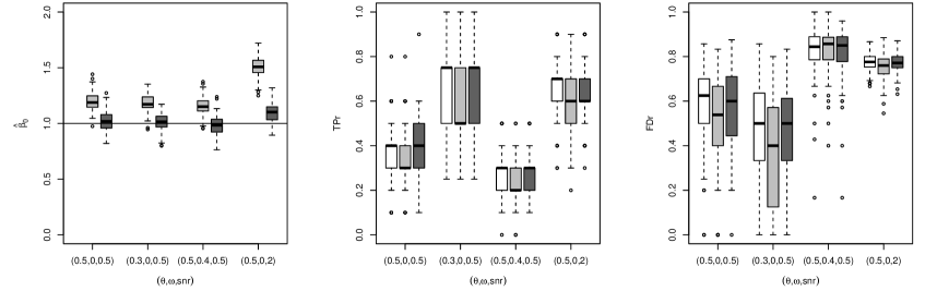
Appendix C Sensitivity study
As noted in Section 5.3, the null-thresholding statistic and therefore the quantile universal threshold are functions of the unknown intercept . In Figure 3, we empirically investigate the sensitivity of our method to the estimation of on the Poisson distributed data of Section 5.2. On the left panel, estimation of (dark grey) described at the end of Section 5.3 has low bias. Moreover we observe the relative median insensitivity of TPr and FDr to the estimate.
Appendix D Phase transition property
We now investigate the variable screening property and observe a phase transition. Given a thresholding estimator, if several tuning parameter values yield containing the true support , the smallest estimated model can be of interest since it minimizes the FDr. We call it the optimal inclusive model. This leads to the definition of the oracle inclusive rate which measures its cardinality relative to the estimated support.
Definition 5.
Assume and let if it exists. Let be the cardinality of . The oracle inclusive rate (OIR) is defined as , where
Models with have , whereas those with have minimum amongst all models with . Moreover, . A small OIr results from a complex model containing , whereas a null OIr results from . The latter could be due to a simplistic model or the variable screening property being unachievable, in which case does not exist.
We extend the simulation of Donoho and Tanner (2010) in compressed sensing to model (4) with unit noise variance assumed to be known. The entries of the matrix are assumed to be i.i.d. standard Gaussian. We set and vary the number of rows as well as the cardinality of the support of , . Nonzero entries are set to ten. One hundred predictor matrices and responses are generated for each pair .
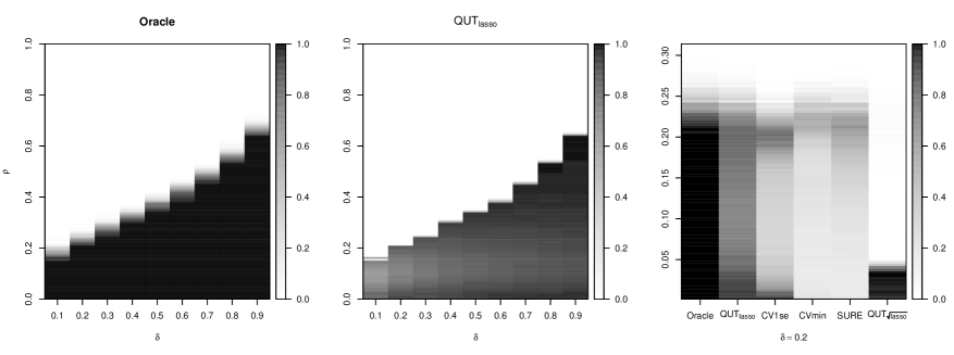
On the left panel of Figure 4, we report OIR for the oracle lasso selection rule which retains the optimal inclusive model if it exists. Values are plotted as a function of , the undersampling factor, and of , the sparsity factor. On the middle and right panel, we report OIR for QUTlasso along other methodologies as well as QUT. The following interesting behaviors are observed:
-
•
Phase transition of Oracle and QUT. Two regions can be clearly distinguished: a high OIR region due to a selected model containing few covariates outside the optimal model and a zero OIR region in which does not exist. The change between these regions is abrupt, as observed in compressed sensing.
-
•
Near oracle performance of QUT. Comparing the left and middle panels, the performance of QUT is nearly as good as that of the oracle selection rule, with the phase transition occurring at similar values of .
-
•
Low complexity of QUTlasso. Comparing several rules on the right panel, QUT has a high OIR. Moreover, CVmin has lower OIR than CV1se and is comparable to SURE. The low OIR of the three latter selection rules is due to the complexity of their selected model. This goes along the fact they are prediction-based methodologies whereas QUT aims at a good identification of the parameters.
-
•
Low OIR of QUT. This could be due to the fact that requires stronger conditions than lasso with a known variance to achieve variable screening (Belloni et al., 2011). Considering its zero-thresholding function, not only its numerator increases as the model deviates from the null model (as lasso), but also its denominator, making screening harder to reach with .
References
- Akaike [1998] H. Akaike. Information theory and an extension of the maximum likelihood principle. In Selected Papers of Hirotugu Akaike, pages 199–213. Springer, 1998.
- Belloni and Chernozhukov [2013] A. Belloni and V. Chernozhukov. Least squares after model selection in high-dimensional sparse models. Bernoulli, 19(2):521–547, 2013.
- Belloni et al. [2011] A. Belloni, V. Chernozhukov, and L. Wang. Square-root lasso: pivotal recovery of sparse signals via conic programming. Biometrika, 98(4):791–806, 2011.
- Breiman et al. [1984] L. Breiman, J. Friedman, R. Olshen, and C. Stone. Classification and Regression Trees. Wadsworth and Brooks/Cole Advanced Books & Software, Monterey, CA, 1984.
- Bühlmann and van de Geer [2011] P. Bühlmann and S. van de Geer. Statistics for High-Dimensional Data: Methods, Theory and Applications. Springer, Heidelberg, 2011.
- Bühlmann et al. [2014] P. Bühlmann, M. Kalisch, and L. Meier. High-dimensional statistics with a view toward applications in biology. Annual Review of Statistics and Its Application, 1:255–278, 2014.
- Bunea et al. [2014] F. Bunea, J. Lederer, and Y. She. The group square-root lasso: theoretical properties and fast algorithms. IEEE Transactions on Information Theory, 60(2):1313–1325, 2014.
- Cai et al. [2010] J.-F. Cai, E. J. Candès, and Z. Shen. A singular value thresholding algorithm for matrix completion. SIAM Journal on Optimization, 20(4):1956–1982, 2010.
- Candès and Romberg [2007] E. Candès and J. Romberg. Sparsity and incoherence in compressive sampling. Inverse Problems, 23(3):969–985, 2007.
- Candès and Tao [2007] E. Candès and T. Tao. The Dantzig selector: statistical estimation when is much larger than . The Annals of Statistics, 35(6):2313–2351, 2007.
- Candès et al. [2013] E. J. Candès, C. A. Sing-Long, and J. D. Trzasko. Unbiased risk estimates for singular value thresholding and spectral estimators. IEEE Transactions on Signal Processing, 61(19):4643–4657, 2013.
- Chen and Chen [2008] J. Chen and Z. Chen. Extended Bayesian information criteria for model selection with large model spaces. Biometrika, 95(3):759–771, 2008.
- Donoho [1995] D. L. Donoho. Nonlinear solution of linear inverse problems by wavelet-vaguelette decomposition. Applied and Computational Harmonic Analysis, 2(2):101–126, 1995.
- Donoho [2006] D. L. Donoho. Compressed sensing. IEEE Transactions on Information Theory, 52(4):1289–1306, 2006.
- Donoho and Johnstone [1994] D. L. Donoho and I. M. Johnstone. Ideal spatial adaptation by wavelet shrinkage. Biometrika, 81(3):425–455, 1994.
- Donoho and Tanner [2010] D. L. Donoho and J. Tanner. Precise undersampling theorems. Proceedings of the IEEE, 98(6):913–924, 2010.
- Donoho et al. [1995] D. L. Donoho, I. M. Johnstone, G. Kerkyacharian, and D. Picard. Wavelet shrinkage: asymptopia? Journal of the Royal Statistical Society: Series B, 57(2):301–369, 1995.
- Donoho et al. [1996] D. L. Donoho, I. M. Johnstone, G. Kerkyacharian, and D. Picard. Density estimation by wavelet thresholding. The Annals of Statistics, 24(2):508–539, 1996.
- Fan and Peng [2004] J. Fan and H. Peng. Nonconcave penalized likelihood with a diverging number of parameters. The Annals of Statistics, 32(3):928–961, 2004.
- Fan et al. [2012] J. Fan, S. Guo, and N. Hao. Variance estimation using refitted cross-validation in ultrahigh dimensional regression. Journal of the Royal Statistical Society: Series B, 74(1):37–65, 2012.
- Fan and Tang [2013] Y. Fan and C. Y. Tang. Tuning parameter selection in high dimensional penalized likelihood. Journal of the Royal Statistical Society: Series B, 75(3):531–552, 2013.
- Fu [1998] W. J. Fu. Penalized regressions: the bridge versus the lasso. Journal of Computational and Graphical Statistics, 7(3):397–416, 1998.
- Gavish and Donoho [2014] M. Gavish and D. L. Donoho. Optimal shrinkage of singular values. arXiv:1405.7511v2, 2014.
- Giacobino [2017] C. Giacobino. Thresholding estimators for high-dimensional data: model selection, testing and existence. PhD thesis, University of Geneva, 2017.
- Golub et al. [1999] T. R. Golub, D. K. Slonim, P. Tamayo, C. Huard, M. Gaasenbeek, J. P. Mesirov, H. Coller, M. L. Loh, J. R. Downing, M. A. Caligiuri, C. D. Bloomfield, and E. S. Lander. Molecular classification of cancer: class discovery and class prediction by gene expression monitoring. Science, 286(5439):531–537, 1999.
- Hoerl and Kennard [1970] A. E. Hoerl and R. W. Kennard. Ridge regression: biased estimation for nonorthogonal problems. Technometrics, 12(1):55–67, 1970.
- James and Stein [1961] W. James and C. Stein. Estimation with quadratic loss. In Proceedings of the Fourth Berkeley Symposium on Mathematical Statistics and Probability, Volume 1: Contributions to the Theory of Statistics, pages 361–379, Berkeley, California, 1961. University of California Press.
- Josse and Husson [2012] J. Josse and F. Husson. Selecting the number of components in PCA using cross-validation approximations. Computational Statististics and Data Analysis, 56(6):1869–1879, 2012.
- Josse and Sardy [2016] J. Josse and S. Sardy. Adaptive shrinkage of singular values. Statistics and Computing, 26(3):715–724, 2016.
- Kushmerick [1999] N. Kushmerick. Learning to remove internet advertisements. In Proceedings of the third international conference on Autonomous Agents, pages 175–181. ACM, 1999.
- Leng et al. [2006] C. Leng, Y. Lin, and G. Wahba. A note on the lasso and related procedures in model selection. Statistica Sinica, 16(4):1273–1284, 2006.
- Mazumder et al. [2010] R. Mazumder, T. Hastie, and R. Tibshirani. Spectral regularization algorithms for learning large incomplete matrices. Journal of Machine Learning Research, 11:2287–2322, 2010.
- Meier et al. [2008] L. Meier, S. van de Geer, and P. Bühlmann. The group lasso for logistic regression. Journal of the Royal Statistical Society, Series B, 70(1):53–71, 2008.
- Meinshausen and Bühlmann [2006] N. Meinshausen and P. Bühlmann. High-dimensional graphs and variable selection with the lasso. The Annals of Statistics, 34:1436–1462, 2006.
- Meinshausen and Bühlmann [2010] N. Meinshausen and P. Bühlmann. Stability selection. Journal of the Royal Statistical Society: Series B, 72(4):417–473, 2010.
- Mukherjee et al. [2015] A. Mukherjee, K. Chen, N. Wang, and J. Zhu. On the degrees of freedom of reduced-rank estimators in multivariate regression. Biometrika, 102(2):457–477, 2015.
- Nelder and Wedderburn [1972] J. A. Nelder and R. W. M. Wedderburn. Generalized linear models. Journal of the Royal Statistical Society: Series A, 135(3):370–384, 1972.
- Neto et al. [2012] D. Neto, S. Sardy, and P. Tseng. -penalized likelihood smoothing and segmentation of volatility processes allowing for abrupt changes. Journal of Computational and Graphical Statistics, 21(1):217–233, 2012.
- Owen and Perry [2009] A. B. Owen and P. O. Perry. Bi-cross-validation of the svd and the nonnegative matrix factorization. Annals of Applied Statistics, 3(2):564–594, 2009.
- Park and Hastie [2007] M. Y. Park and T. Hastie. -regularization-path algorithm for generalized linear models. Journal of the Royal Statistical Society: Series B, 69(4):659–677, 2007.
- Pitman and Yor [1999] J. Pitman and M. Yor. The law of the maximum of a bessel bridge. Electronic Journal of Probability, 4:1–35, 1999.
- Reid et al. [2014] S. Reid, R. Tibshirani, and J. Friedman. A study of error variance estimation in lasso regression. arXiv:1311.5274v2, 2014.
- Rockafellar [1970] R. T. Rockafellar. Convex Analysis. Princeton University Press, Princeton, 1970.
- Rudin et al. [1992] L. I. Rudin, S. Osher, and E. Fatemi. Nonlinear total variation based noise removal algorithms. Physica D, 60:259–268, 1992.
- Sardy [2008] S. Sardy. On the practice of rescaling covariates. International Statistical Review, 76(2):285–297, 2008.
- Sardy [2009] S. Sardy. Adaptive posterior mode estimation of a sparse sequence for model selection. Scandinavian Journal of Statistics, 36(4):577–601, 2009.
- Sardy [2012] S. Sardy. Smooth blockwise iterative thresholding: a smooth fixed point estimator based on the likelihood’s block gradient. Journal of the American Statistical Association, 107(498):800–813, 2012.
- Sardy and Tseng [2004] S. Sardy and P. Tseng. On the statistical analysis of smoothing by maximizing dirty markov random field posterior distributions. Journal of the American Statistical Association, 99(465):191–204, 2004.
- Sardy and Tseng [2010] S. Sardy and P. Tseng. Density estimation by total variation penalized likelihood driven by the sparsity information criterion. Scandinavian Journal of Statistics, 37(2):321–337, 2010.
- Sardy et al. [2004] S. Sardy, A. Antoniadis, and P. Tseng. Automatic smoothing with wavelets for a wide class of distributions. Journal of Computational and Graphical Statistics, 13(2):399–421, 2004.
- Schwarz [1978] G. Schwarz. Estimating the dimension of a model. The Annals of Statistics, 6(2):461–464, 1978.
- Simon et al. [2013] N. Simon, J. Friedman, T. Hastie, and R. Tibshirani. A sparse-group lasso. Journal of Computational and Graphical Statistics, 22(2):231–245, 2013.
- Stein [1981] C. M. Stein. Estimation of the mean of a multivariate normal distribution. The Annals of Statistics, 9(6):1135–1151, 1981.
- Tibshirani [1996] R. Tibshirani. Regression shrinkage and selection via the lasso. Journal of the Royal Statistical Society, Series B, 58(1):267–288, 1996.
- Tibshirani et al. [2005] R. Tibshirani, M. Saunders, S. Rosset, J. Zhu, and K. Knight. Sparsity and smoothness via the fused lasso. Journal of the Royal Statistical Society, Series B, 67(1):91–108, 2005.
- Tibshirani and Taylor [2011] R. J. Tibshirani and J. Taylor. The solution path of the generalized lasso. The Annals of Statistics, 39(3):1335–1371, 2011.
- Tibshirani and Taylor [2012] R. J. Tibshirani and J. Taylor. Degrees of freedom in lasso problems. The Annals of Statistics, 40(2):1198–1232, 2012.
- Tikhonov [1963] A. N. Tikhonov. Solution of incorrectly formulated problems and the regularization method. Soviet Mathematics Doklady, 4(4):1035–1038, 1963.
- Wahba [1990] G. Wahba. Spline Models for Observational Data. Society for Industrial and Applied Mathematics, Philadelphia, 1990.
- Wang et al. [2007] H. Wang, G. Li, and G. Jiang. Robust regression shrinkage and consistent variable selection through the LAD-lasso. Journal of Business & Economic Statistics, 25(3):347–355, 2007.
- Yang [2005] Y. Yang. Can the strengths of AIC and BIC be shared? A conflict between model indentification and regression estimation. Biometrika, 92(4):937–950, 2005.
- Yuan and Lin [2006] M. Yuan and Y. Lin. Model selection and estimation in regression with grouped variables. Journal of the Royal Statistical Society, Series B, 68(1):49–67, 2006.
- Zhang [2010] C.-H. Zhang. Nearly unbiased variable selection under minimax concave penalty. The Annals of Statistics, 38(2):894–942, 2010.
- Zou [2006] H. Zou. The adaptive lasso and its oracle properties. Journal of the American Statistical Association, 101(476):1418–1429, 2006.
- Zou and Hastie [2005] H. Zou and T. Hastie. Regularization and variable selection via the elastic net. Journal of the Royal Statistical Society: Series B, 67(2):301–320, 2005.
- Zou et al. [2007] H. Zou, T. Hastie, and R. Tibshirani. On the “degrees of freedom” of the lasso. The Annals of Statistics, 35(5):2173–2192, 2007.