Space-filling curves of self-similar sets (II): Edge-to-trail substitution rule

Abstract.

It is well-known that the constructions of space-filling curves depend on certain substitution rules. For a given self-similar set, finding such rules is somehow mysterious, and it is the main concern of the present paper.

Our first idea is to introduce the notion of skeleton for a self-similar set. Then, from a skeleton, we construct several graphs, define edge-to-trail substitution rules, and explore conditions ensuring the rules lead to space-filling curves. Thirdly, we summarize the classical constructions of the space-filling curves into two classes: the traveling-trail class and the positive Euler-tour class. Finally, we propose a general Euler-tour method, using which we show that if a self-similar set satisfies the open set condition and possesses a skeleton, then space-filling curves can be constructed. Especially, all connected self-similar sets of finite type fall into this class. Our study actually provides an algorithm to construct space-filling curves of self-similar sets.

MSC 2000: 28A80, 54C05.

1. Introduction

Space-filling curves (SFC) have fascinated mathematicians for over a century since Peano’s monumental work in 1890. In a series of three papers ([35], the present paper, and [36]), we develop a theory to construct SFCs of self-similar sets. For a given connected self-similar set, finding substitution rules leading to SFCs is a long-standing and difficult problem, and it is the main concern of the present paper.

1.1. A brief history of space-filling curves.

SFCs of the first generation were constructed by Peano (1890), Hilbert (1891), Sierpiński (1912) and Pólya (1913) ([30, 18, 40, 31]), where the base sets are squares or triangles. Later on, people found many beautiful reptiles as well as their space-filling curves, where the boundaries of the reptiles are fractals; for instance, Heighway dragon curve ([10]), Gosper curve ([16]), etc.. A survey of the early results can be found in Sagan [38]. In recent years, various interesting SFCs appear on the internet, see for example, “www.fractalcurves.com” ([47]) and “teachout1.net/village/” ([44]). Figure 2 illustrates two of them.

From the 1960’s to the 1980’s, two systematic methods were introduced to handle the SFCs. The first one is the $L$-system method introduced by Lindenmayer ([24]), a biologist; this method is known to a very wide audience, see Bader [5]. The second method is the recurrent set method introduced by Dekking [11], which is an improvement of the $L$-system method. See [35] for the comparing of the two methods.

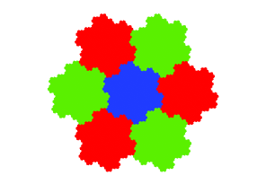
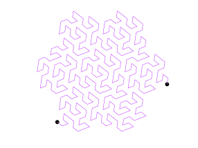
Figure 1. Gosper island and Gosper curve.

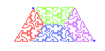
(a) Wedge tile

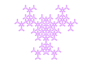
(b) Four-tile star

Figure 2. Two SFCs taking from [44]: (a) is discussed in Example 4.1, and a detailed discussion of (b) is given in Section 7 of [35].

All the known constructions of SFC depend on certain ‘substitution rules’. Indeed, the $L$-system method and the recurrent set method provide exact meaning of ‘substitution rule’ and build a bridge from substitution rules to SFCs, but they do not tell us how to construct substitution rules.

There are few works on the construction of substitution rules. Hata [17] shows that if a self-similar set is generated by a linear IFS (see Section 4 for the definition), then a substitution rule can be obtained. Another way is to consider the attractor of the so-called path-on-lattice IFS (this name is given by [35]). A path on a planar lattice defines a substitution rule as well as a self-similar set; if the self-similar set happens to satisfy the open set condition, then the substitution rule leads to a SFC. This method is widely used to find reptiles and space-filling curves by computer searching, see Fukuda et al. [15], Arndt [2] and “www.fractalcurves.com” [47]. But in this method, the self-similar sets are not priori given. Other attempts of constructing substitution rules for special self-similar sets can be found in Remes [37] and Sirvent [41, 42, 43].

Before stating our results, we note that as we did in [35], the terminology ‘space-filling curve’ is used in a strong sense, that is, it is a kind of optimal parametrization. Let ${\mathcal{H}}^{s}$ denote the $s$-dimensional Hausdorff measure.

Definition 1.1.

Let $K$ be a compact subset of ${\mathbb{R}}^{d}$ with $0<{\mathcal{H}}^{s}(K)<\infty$. An onto mapping $\psi:[0,1]\rightarrow K$ is called an optimal parametrization of $K$ if:

$(i)$ $\psi$ is almost one-to-one, that is, there exist $K^{\prime}\subset K$ and $I^{\prime}\subset[0,1]$ with full measures such that $\psi:~{}I^{\prime}\to K^{\prime}$ is a bijection;

$(ii)$ $\psi$ is measure-preserving in the sense that

$${\mathcal{H}}^{s}(\psi(F))=c{\mathcal{L}}(F)\text{ and }{\mathcal{L}}(\psi^{-1}(B))=c^{-1}{\mathcal{H}}^{s}(B),$$

for any Borel set $F\subset[0,1]$ and any Borel set $B\subset K$, where $c={\mathcal{H}}^{s}(K)$.

$(iii)$ $\psi$ is $1/s$-Hölder continuous, that is, there is a constant $c^{\prime}>0$ such that

$$|\psi(x)-\psi(y)|\leq c^{\prime}|x-y|^{\frac{1}{s}}\ \text{ for all }x,y\in[0,1].$$

Recall that a non-empty compact set $K\subset\mathbb{R}^{d}$ is called a self-similar set, if there exist contractive similitudes $S_{1},\dots,S_{N}:\mathbb{R}^{d}\to\mathbb{R}^{d}$ such that

$$K=\bigcup_{j=1}^{N}S_{j}(K).$$

The family $\{S_{1},\dots,S_{N}\}$ is called an iterated function system, or IFS in short; $K$ is called the invariant set of the IFS. (See for instance, [19, 14]). The IFS $\{S_{1},\dots,S_{N}\}$ is said to satisfy the open set condition (OSC), if there is an open set $U$ such that $\bigcup_{i=1}^{N}S_{i}(U)\subset U$ and the sets $S_{i}(U)$ are disjoint ([19]). If a self-similar set $K$ satisfies the OSC and has non-empty interior, then we call $K$ a self-similar tile; if in addition, the contraction ratios of $S_{i}$ are all equal , then $K$ is called a reptile ([20]).

In this paper, we introduce a new notion, called skeleton of a self-similar set, which is crucial in our theory. As soon as we have a skeleton, we construct a space-filling curve along the following line:

Skeleton $\rightarrow$ graphs and edge-to-trail substitution $\rightarrow$ space-filling curve $\rightarrow$ visualization.

To ‘see’ a SFC, we need to visualize or to approximate the curve, and this has been studied in [35]. In the following, we give a brief description of the first three steps.

1.2. Skeleton of a self-similar set

Let $\{S_{j}\}_{j=1}^{N}$ be an IFS with invariant set $K$. Let $A$ be a finite subset of $K$. We call $A$ a skeleton if it satisfies the following two conditions:

$(i)$ It is stable under iteration, that is, $A\subset\bigcup_{j=1}^{N}S_{j}(A)$;

$(ii)$ It is a representative with respect to the connectedness, that is, the so-called Hata graph associated with $A$ is connected. (See Section 2 for the precise definition.)

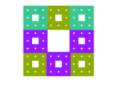
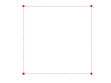
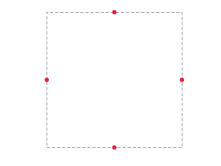
Figure 3. The Sierpiński carpet and two skeletons of it.

From now on, we always assume that $K$ is a connected self-similar set possessing a skeleton which we denote by

(1.1) $$A=\{a_{1},\dots,a_{m}\}.$$

1.3. Graphs and edge-to-trail substitution

First, we recall some terminologies of graph theory, see for instance, [6]. Let $H$ be a directed graph. We shall use $e_{1}+\dots+e_{k}$ to denote a walk consisting of the edges $e_{1},\dots,e_{k}$. We call the starting vertex and terminate vertex of a walk the origin and terminus, respectively. The walk is closed if the origin of $e_{1}$ and the terminus of $e_{k}$ coincide.

A walk is called a trail, if all the edges appearing in the walk are distinct. A trail is called a path if all the vertices are distinct. A closed path is called a cycle.

A subgraph $H^{\prime}$ of $H$ is called spanning, if $H^{\prime}$ contains all the vertices of $H$. An Euler trail in $H$ is a spanning trail in $H$ that contains all the edges of $H$. An Euler tour of $H$ is a closed Euler trail of $H$.

(a) Terdragon

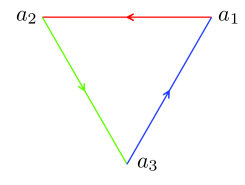
(b) Initial graph

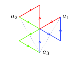
(c) Refined graph

Figure 4. An edge-to-trail substitution for Terdragon: an edge in (b) maps to the trail in (c) with the same color. Detail is given in Example 4.

Using the skeleton $A=\{a_{1},\dots,a_{m}\}$, we define

(1.2) $$G_{0}=\{\overrightarrow{a_{i}a_{j}};1\leq i,j\leq m\}$$

which is the directed complete graph with vertex set $A$.

We select a spanning subgraph $\Lambda=(A,V)$ of $G_{0}$ as the initial graph of our construction, where $A$ is the vertex set and $V$ is the edge set. Let $G$ be the union of affine images of $V$ under $S_{j}$, i.e.,

(1.3) $$G=\bigcup_{j=1}^{N}S_{j}(\Lambda).$$

We call $G$ the refined graph induced by $\Lambda$. (See Section 3.)

If for each edge $u\in V$, we can find a trail $P_{u}$ in $G$ which shares the origin and terminus with $u$, then we call the mapping

$$u\mapsto P_{u},u\in V$$

an edge-to-trail substitution.

1.4. Feasible edge-to-trail substitutions

Now we investigate when a rule $\tau$ leads to a space-filling curve, or equivalently, an optimal parametrization. Rao and Zhang [35] introduce linear graph-directed iterated function system (linear GIFS), which provides a criterion for optimal parameterizations. (See also Section 6.)

Theorem 1.1.

([35]) Let $\{E_{j}\}_{j=1}^{N}$ be the invariant sets of a linear GIFS satisfying the open set condition and $0<\mathcal{H}^{\delta}(E_{j})<\infty$ for $1\leq j\leq N$, where $\delta$ is the similarity dimension. Then $E_{j}$ admits optimal parameterizations for every $j=1,\dots,N$.

An edge-to-trail substitution induces a linear GIFS in a nature way (Theorem 7.1). We will impose conditions on edge-to-trail substitutions so that Theorem 1.1 can be applied.

First, using our point of view, we summarize the constructions of SFC in the literature into two classes, the traveling-trail method and the positive Euler-tour method, and provide a rigorous treatment to them.

(1) Traveling-trail method and self-similar zippers.

A trail of length $N$ in the refined graph $G=\bigcup_{j=1}^{N}S_{j}(\Lambda)$ is called a traveling trail, if for every $j\in\{1,\dots,N\}$, the trail contains exactly one edge in $S_{j}(\Lambda)$. We show that

Theorem 1.2.

If all the trails $P_{u}$ in a edge-to-trail substitution $\tau$ are traveling trails, then $\tau$ leads to a space-filling curve of $K$.

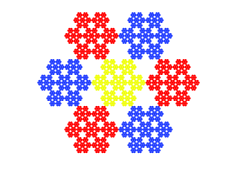
(a) Hexaflake fractal.

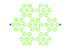
(b) By traveling-trail method.

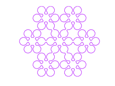
(c) By Euler-tour method.

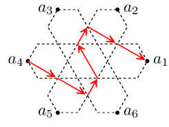
(d) Traveling trail from $a_{4}$ to $a_{1}$

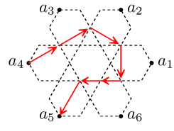
(e) Traveling trail from $a_{4}$ to $a_{5}$

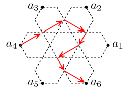
(f) Traveling trail from $a_{4}$ to $a_{6}$

Figure 5. Applying the traveling-trail method, we construct a space-filling curve of the Hexaflake fractal, see Figure (b). The details are given in Example 4.2. The Hexaflake can also be parameterized by the positive Euler-tour method, see Figure (c).

The following SFCs are constructed by this method (see Section 4): Peano curve, Hilbert curve, Heighway dragon curve, Gosper curve, curves in Fukuda et al. [15] and the web-sites [47, 44].

A special class of IFS, called self-similar zipper, is first introduced by Thurston ([46]) and plays a role in complex analysis ([4]). Recently, there are some works on self-similar zippers on the fractal aspect [3, 32, 45].

Definition 1.2.

Let $(S_{j})_{j=1}^{N}$ be an IFS where the mappings are ordered. If there exists a set $\{x_{0},\dots,x_{N}\}$ of points and a sequence $(\beta_{1},\dots,\beta_{N})\in\{-1,1\}^{N}$, such that the mapping $S_{j}$ takes the pair $(x_{0},x_{n})$ either into the pair $(x_{j-1},x_{j})$ if $s_{j}=1$ or into the pair $(x_{j},x_{j-1})$ if $s_{j}=-1$, then we call $(S_{j})_{n=1}^{N}$ a self-similar zipper.

We call $\{x_{0},\dots,x_{N}\}$ the set of vertices and call $(\beta_{1},\dots,\beta_{N})$ the vector of signature.

Indeed, there is a one-to-one correspondence between self-similar zippers and ‘symmetric’ linear GIFS with two states.

Theorem 1.3.

An IFS $(S_{i})_{i=1}^{N}$ is a self-similar zipper with signature $(\beta_{1},\dots,\beta_{N})$ if and only if the following ordered GIFS with two states

(1.4) $$\left\{\begin{split}E_{1}=&S_{1}(E_{\beta_{1}})+S_{2}(E_{\beta_{2}})+\dots+S_{N}(E_{\beta_{N}}),\\ E_{-1}=&S_{N}(E_{-\beta_{N}})+S_{N-1}(E_{-\beta_{N-1}})+\dots+S_{1}(E_{-\beta_{1}})\end{split}\right.$$

is a linear GIFS. If the OSC holds in addition, then the invariant set $K$ of $(S_{i})_{i=1}^{N}$ admits optimal parameterizations.

This theorem is proved in Section 6. Actually, the proof gives us an easy algorithm to determine whether an IFS is a zipper or not.

(2) Positive Euler-tour method.

A natural selection of the initial graph is $\Lambda=\overrightarrow{a_{1}a_{2}}+\dots+\overrightarrow{a_{m-1}a_{m}}+\overrightarrow{a_{m}a_{1}},$ the cycle passing all the elements of $A$. Next, we choose an Euler tour of the refined graph $G$ and a partition of this Euler tour. This partition can give us an edge-to-trail substitution, if a consistency condition is fulfilled (see Section 8). Besides, we pose two more conditions: the primitivity condition and pure-cell condition. We show that if these conditions are fulfilled, then the associated edge-to-trail substitution leads to a SFC of $K$ (Theorem 8.2).

The following curves are constructed by this method: Sierpiński curve, Terdragon curve in Dekking [11], the four-tile star in [44] (see Figure 2(b)). In this paper, we present two new examples: Sierpiński carpet (Example 5.2) and the Rocket tile (Example 5.3).

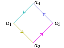
(a) Initial graph.

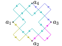
(b) Euler tour.

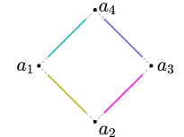
(c) Initial patterns.

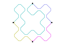
(d) The first iteration.

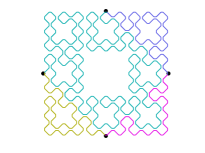
(e) The second interation.

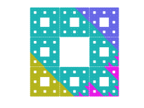
(f) Invariant sets of GIFS.

Figure 6. A space-filling curve of the Sierpiński carpet.

Does every self-similar sets admit space-filling curves? To answer this question, we introduce a general Euler-tour method.

(3) (General) Euler-tour method.

Let $\Lambda^{-1}$ be the reverse cycle of $\Lambda$ in the positive Euler-tour method. Now, in the refined graph $G$, we allow negative orientation, that is, for some $j$, we replace $S_{j}(\Lambda)$ by $S_{j}(\Lambda^{-1})$. Then we have much more choices, which produce more refined graphs and Euler tours, and increases the possibility of finding a feasible edge-to-trail substitution. We show that

Theorem 1.4.

Let $\{S_{j}\}_{j=1}^{N}$ be an IFS possessing skeletons and satisfying the open set condition. Then the invariant set $K$ admits space-filling curves. More precisely, either an rearrangement of $\{S_{j}\}_{j=1}^{N}$ is a self-similar zipper, or $K$ admits space-filling curves constructed by the Euler-tour method.

The difficult part of Theorem 1.4 is to prove the non self-similar zipper case, which we divide into two steps. First, we prove Theorem 8.2, which transfers the space-filling curve problem to a graph theory problem. Then, we solve the graph theory problem in Section 9 and 10, where we use a bubbling process to produce the desired Euler tour and then make a suitable choice of orientations of the basic cells.

Self-similar sets of finite type is an important class of fractals, see for instance, [34, 25, 7]. In a subsequent paper [36], we show that if $K$ is a self-similar set of finite type, then $K$ possesses skeletons. Consequently, we have

Theorem 1.5.

Let $K$ be a connected self-similar set of finite type and satisfying the open set condition. Then $K$ admits space-filling curves.

Example 1.1.

Integral self-affine tiles. Let $A$ be an integral $n\times n$ expanding matrix, and $D\subset{\mathbb{Z}}^{n}$ be a set with $\#D=|\det A|$, where $\#D$ denotes the cardinality of $D$. Let $T$ be the unique compact set satisfying

$$AT=\bigcup_{d\in D}T+D.$$

The set $T$ is called an integeral self-affine tile if it has positive Lebesgue measure. (See Lagarias and Wang [22] and the reference therein). By Theorem 1.5, every integral self-affine tile admits space-filling curves.

The Rocket tile is taken from Duvall et al. [13]. It is an integral self-similar tile with $9$ branches. A SFC is shown in Figure 7. The details are given in Example 5.3.

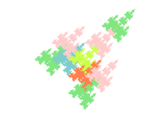
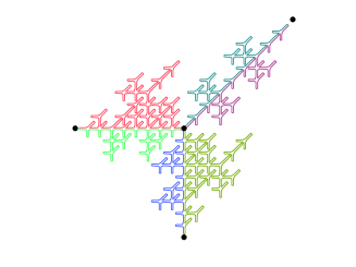
Figure 7. A space-filling curve of the Rocket tile.

Example 1.2.

The Christmas tree. The Christmas tree is a fractal with $5$ branches. Figure 13 provides a space-filling curve of it, where the negative orientation is involved; the details are given in Example 8.4. It can be parameterized with the positive Euler-tour method, but the parametrization is not measure-preserving, since the edge-to-trail substitution cannot be primitive.

The paper is organized as follows. In Section 2, we give a brief description of skeletons of self-similar sets. In Section 3, we describe the general philosophy of constructing edge-to-trail substitutions by graphs. Section 4 and Section 5 are devoted to the traveling-trail method and the positive Euler-tour method, respectively. In Section 6 and Section 7, we show an induced GIFS is always a linear GIFS, and Theorem 1.2 is proved there. Section 8-11 are devoted to the Euler-tour method, and Theorem 1.4 is proved in Section 11.

2. Skeleton of self-similar set

In this section, we give a brief introduction to skeletons of self-similar sets. A detailed study is carried out in Rao and Zhang [36].

Let ${\mathcal{S}}=\{S_{j}\}_{j=1}^{N}$ be an IFS with invariant set $K$. For any subset $A$ of $K$, we define a graph $H(A)$ as following: The vertex set is $\{S_{1},S_{2},\dots,S_{N}\}$, and there is an edge between two vertices $S_{i}$ and $S_{j}$ if and only if $S_{i}(A)\cap S_{j}(A)\neq\emptyset$. We call $H(A)$ the Hata graph induced by $A$.

Remark 2.1.

Such graphs are first studied by Hata [17], where he proved that a self-similar set $K$ is connected if and only if the graph $H(K)$ is connected.

Definition 2.1.

Let $K$ be a connected self-similar set, and let $A$ be a finite subset of $K$. We call $A$ a skeleton of $\{S_{j}\}_{j=1}^{N}$ (or $K$), if $A\subset\bigcup_{j=1}^{N}S_{j}(A)$ and the Hata graph $H(A)$ is connected.

Remark 2.2.

Kigami [21] and Morán [28] have studied the ‘boundary’ (also called ’vertices’ if it is finite) of a fractal. A skeleton is usually chosen to be a subset of the ‘boundary’ of a self-similar set since we want a small skeleton; for a so-called p.c.f. self-similar set, the set of vertices is a skeleton. Indeed, the choices of skeletons are much more arbitrary.

2.1. Iteration

We denote $\Sigma=\{1,\dots,N\}$ and call it an alphabet. Let $I=i_{1}i_{2}\dots i_{n}\in\Sigma^{n}$, we call it a word of length $n$. We denote the length of a word $I$ by $|I|$. We define the $n$-th iteration of $\mathcal{S}$ to be the IFS

$${\mathcal{S}}^{n}=\{S_{I};~{}I\in\Sigma^{n}\},$$

where

$$S_{I}=S_{i_{1}}\circ S_{i_{2}}\circ\cdots\circ S_{i_{n}},\quad\text{ if }I=i_{1}\dots i_{n}.$$

It is well-known that the invariant set $K$ of the IFS ${\mathcal{S}}$ is also the invariant set of ${\mathcal{S}}^{n}$ (see Falconer [14]). Similarly, we have

Proposition 2.3.

([36]) If $A$ is a skeleton of $\mathcal{S}$, then $A$ is also a skeleton of $\mathcal{S}^{n}$.

Using neighbour graph of self-similar sets, it is shown ([36]) that a connected self-similar set of finite type always possesses skeletons, and actually an algorithm of finding skeletons is given there. There do exist self-similar sets without skeletons.

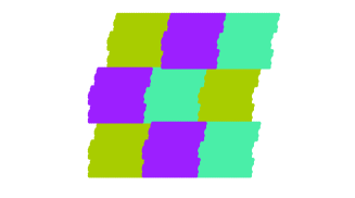
Figure 8. A reptile without skeleton, see [36].

3. Graphs and edge-to-trail substitutions: the general philosophy

Let $\mathcal{S}=\{S_{j}\}_{j=1}^{N}$ be an IFS possessing a skeleton and satisfying the OSC. Let us denote its invariant set by $K$, and let $A=\{a_{1},a_{2},\dots,a_{m}\}$ be a skeleton. Recall

$$G_{0}=\{\overrightarrow{a_{i}a_{j}};~{}1\leq i,j\leq m\},$$

is a directed complete graph with vertex set $A$. We note that the edges $\overrightarrow{a_{i}a_{j}}$ are abstract edges rather than oriented line segments; moreover, $i$ may be equal to $j$, see Example 4.1.

Next, we choose a subgraph $\Lambda=(A,V)$ of $G_{0}$, and we call $\Lambda$ the initial graph. To continue our construction, we need to define the affine copy of a directed graph.

Definition 3.1.

Let $G=(\mathcal{A},\Gamma)$ be a directed graph such that the vertex set $\mathcal{A}\subset\mathbb{R}^{d}$. Let $S:{\mathbb{R}}^{d}\to\mathbb{R}^{d}$ be a affine mapping. We define a directed graph $G_{S}=(S(\mathcal{A}),\Gamma_{S})$ as follows: there is an edge in $\Gamma_{S}$ from $S(x)$ to $S(y)$, if and only if there is an edge $e\in\Gamma$ from vertex $x$ to $y$. Moreover, we denote this edge by $(e,S)$. For simplicity, we shall denote $G_{S},\Gamma_{S},$ and $(e,S)$ by $S(G),S(\Gamma)$ and $S(e)$, respectively.

Remark 3.1.

(i) If $(\mathcal{A}_{1},\Gamma_{1})$ and $(\mathcal{A}_{2},\Gamma_{2})$ are two graphs without common edges, then we define their union to be the graph $(\mathcal{A}_{1}\cup\mathcal{A}_{2},\Gamma_{1}\cup\Gamma_{2})$.

(ii) Even if $S_{j}(e_{k})$ coincides with $S_{j^{\prime}}(e_{k^{\prime}})$ as oriented line segment, they should regarded as different edges, since $(e_{k},S_{j})\neq(e_{k^{\prime}},S_{j^{\prime}})$.

3.1. Refined graph and edge-to-trail substitution

Let $G$ be the union of affine images of $\Lambda$ under $S_{j}$, that is,

(3.1) $$G=\bigcup_{j=1}^{N}S_{j}(\Lambda),$$

and we call it the refined graph induced by $\Lambda$.

Let $\tau$ be a mapping from $V$ to trails of $G$; we shall denote $\tau(u)$ by $P_{u}$ to emphasize that $\tau(u)$ is a trail. We call $\tau$ an edge-to-trail substitution, if for all $u\in V$, $P_{u}$ has the same origin and terminus as $u$.

An edge-to-trail substitution $\tau$ can be thought as replacing each big edge $u$ by a trail $P_{u}$ consisting of small edges. Our goal is to construct feasible edge-to-trail substitutions which lead to SFCs.

3.2. Iteration of edge-to-trail substitutions

We use the following two rules to iterate $\tau$:

(i) For $I\in\bigcup_{n\geq 1}\{1,2,\dots,N\}^{n}$ and $u\in V$, if $\tau(u)=\gamma_{1}+\dots+\gamma_{\ell}$, we set

(3.2) $$\tau(S_{I}(u))=S_{I}(\gamma_{1})+\dots+S_{I}(\gamma_{\ell});$$

(ii) Set

$$\tau(w_{1}+w_{2}+\dots+w_{k})=\tau(w_{1})+\tau(w_{2})+\dots+\tau(w_{k})$$

if $w_{j}\in\{S_{I}(v);I\in\{1,2,\dots,N\}^{n},v\in V\}$ for some $n$.

Hence, we can define $\tau^{n}(u)$ recurrently, which is a trail consisting of small edges. Geometrically, we can explain $\tau^{n}(u)$ as an oriented broken line which provides an approximation of the corresponding SFC.

4. Traveling-trail method

Recall that a trail $P$ in $G=\bigcup_{j=1}^{N}S_{j}(\Lambda)$ is called a traveling trail, if for every $j$, $P$ contains exactly one edge in $S_{j}(\Lambda)$. Theorem 1.2 asserts that if all the trails $P_{u}$ in a edge-to-trail substitution $\tau$ are traveling trails, then $\tau$ leads to a SFC of $K$. We postpone the proof of Theorem 1.2 to Section 7. In this section, we summarize the SFCs constructed by this method.

4.1. Linear IFS

Let $K$ be a self-similar set. Assume that $K$ has a skeleton consisting of two points, say $A=\{a,b\}$. Denote $u=\overrightarrow{ab}$ and let $V=\{u\}$. If $S_{1}(u)+\cdots+S_{N}(u)$ is a trail from $a$ to $b$, where we use the symbol ‘+’ to connect the consecutive edges or sub-trails, then

(4.1) $$\tau:u\mapsto S_{1}(u)+\cdots+S_{N}(u)$$

is a feasible edge-to-trail substitution, since $\tau(u)$ is a traveling trail. Such IFS, called a linear IFS in [35], was first studied by De Rahm [12] and Hata [17], where they proved that a linear IFS leads to a SFC, which is a direct generalization of Peano’s original construction.

4.2. Self-similar zipper

Let $K$ be the invariant set of a self-similar zipper $\{S_{j}\}_{j=1}^{N}$ with vertices $\{x_{0},\dots,x_{N}\}$ and signature $\{\beta_{1},\dots,\beta_{N}\}$. Then $K$ possesses a skeleton $A=\{x_{0},x_{N}\}$. Denotes $u=\overrightarrow{x_{0}x_{N}}$ and set $V=\{u,u^{-1}\}$, where $u^{-1}$ denote the reverse edge of $u$. Clearly

$$\tau:\left\{\begin{array}[]{rl}u&\mapsto S_{1}(u^{\beta_{1}})+\cdots+S_{N}(u^{\beta_{N}})\\ \quad u^{-1}&\mapsto\text{reverse trail of }S_{1}(u^{\beta_{1}})+\cdots+S_{N}(u^{\beta_{N}})\end{array}\right.$$

is a feasible edge-to-trail substitution since both $\tau(u)$ and $\tau(u^{-1})$ are traveling trails. (The path-on-lattice IFS in [35] is a special case of the self-similar zipper). Hilbert curve, Heighway dragon curve and Gosper curve are obtained by this way. See Section 5 of [35] for details.

4.3. Space-filling curves of polygonal reptiles.

In the web-site Teachout [44], there are many interesting SFCs of polygonal reptiles. These curves are obtained by traveling-trail method. We take the Wedge tile as an example.

Example 4.1.

The Wedge Tile. The Wedge tile is a self-similar set generated by the IFS $\{S_{i}\}_{i=1}^{4}$, where the maps are indicated by Figure 9(a),(b). (Here we use an arrow to specify the linear part of $S_{j}$ contains reflection or not. )

We choose $A=\{a_{2},a_{4}\}$, two vertices of the wedge, to be the skeleton. Choose

$$V=\{\overrightarrow{a_{4}a_{2}},\overrightarrow{a_{2}a_{4}},\overrightarrow{a_{4}a_{4}}\}=:\{\alpha,\beta,\gamma\}.$$

Then

$$\tau:~{}\left\{\begin{array}[]{rl}\alpha&\mapsto S_{1}(\beta)+S_{2}(\beta)+S_{3}(\gamma)+S_{4}(\alpha),\\ \beta&\mapsto S_{4}(\beta)+S_{3}(\gamma)+S_{2}(\alpha)+S_{1}(\alpha),\\ \gamma&\mapsto S_{3}(\beta)+S_{4}(\gamma)+S_{2}(\alpha)+S_{1}(\alpha)\end{array}\right.$$

is an edge-to-trail substitution. The trails $\tau(\alpha)$ and $\tau(\gamma)$ are illustrated by Figure 9(c) and (d); the trail $\tau(\beta)$ is the reverse trail of $\tau(\alpha)$. A visualization of the SFC corresponding to $\tau$ is shown in Figure 2(a).

(a)

(b)

(c) A trail from $a_{4}$ to $a_{2}$.

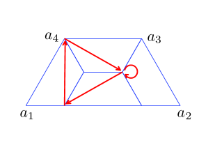
(d) A closed trail from $a_{4}$ to $a_{4}$.

Figure 9.

Example 4.2.

Hexaflake. Hexaflake is a fractal constructed by iteratively exchanging each hexagon by a flake of seven hexagons, see Figure 5 (a). We choose $A$ to be the vertex set of the original hexagon, and choose the initial graph to be

$$V=\{\overrightarrow{a_{i}a_{j}};~{}i\neq j\}.$$

Figure 5 (d)(e)(f) show the trails for $\overrightarrow{a_{4}a_{1}}$, $\overrightarrow{a_{4}a_{5}}$ and $\overrightarrow{a_{4}a_{6}}$. For any $\overrightarrow{a_{i}a_{j}}$, there is a similitude which maps one of $\overrightarrow{a_{4}a_{1}}$, $\overrightarrow{a_{4}a_{5}}$ and $\overrightarrow{a_{4}a_{6}}$ to $\overrightarrow{a_{i}a_{j}}$, and hence this similitude induces a trail which we define to be $\tau(\overrightarrow{a_{i}a_{j}})$. The rule $\tau$ satisfies the condition of Theorem 1.2. Figure 5(b) gives a visualization of the corresponding SFC.

A more popular sFC of Hexaflake is coustructed by the positive Euler-tour method, see Figure 5(c).

5. Positive Euler-tour method

Another frequently used method of constructing SFC is the positive Euler-tour method. Let $A=\{a_{1},\dots,a_{m}\}$ be a skeleton. Define

(5.1) $$\Lambda=\Lambda_{A}:=\overrightarrow{a_{1}a_{2}}+\cdots+\overrightarrow{a_{m-1}a_{m}}+\overrightarrow{a_{m}a_{1}}$$

to be the cycle passing $a_{1},\dots,a_{m}$ in turn. We denote the edge set of $\Lambda$ by

$$V^{+}=\{\overrightarrow{a_{1}a_{2}},\dots,\overrightarrow{a_{m-1}a_{m}},\overrightarrow{a_{m}a_{1}}\}.$$

We set $\Lambda$ to be our initial graph, and let $G=\bigcup_{i=1}^{N}S_{j}(\Lambda)$ be the refined graph.

Lemma 5.1.

The refine graph $G$ admits Euler tours.

Proof.

First, we prove $G$ is connected. Take two vertices $S_{i}(a)$ and $S_{j}(b)$ in $G$, where $a,b\in A$. Let $S_{i}=S_{i_{0}},S_{i_{1}},\dots,S_{i_{k}}=S_{j}$ be the vertices of a path connecting $S_{i}$ and $S_{j}$ in the Hata graph $H({\mathcal{S}},A)$. Then one can easily prove by induction that the graphs

$$S_{i_{0}}(\Lambda)\cup\cdots\cup S_{i_{\ell}}(\Lambda),\quad 0\leq\ell\leq k,$$

are all connected. Set $\ell=k$, we get that $G$ is connected.

Finally, $G$ admits Euler tour, since it is a disjoint union of closed trails (see [8]). ∎

Let $P$ be an Euler tour of the refined graph $G$. Let $P=P_{1}+\cdots+P_{m}$ be a partition of $P$ such that that for all $j$, $P_{j}$ is a sub-trail having the same origin and terminus as $v_{j}$. Then

$$\tau:v_{j}\mapsto P_{j},\quad j=1,2,\dots,m,$$

gives us an edge-to-trail substitution. If $P$ and the partition are carefully chosen, then $\tau$ will lead to a SFC. The rigorious treatment is given in Section 8.

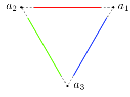
(a) Initial pattern

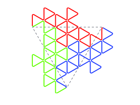
(b) The second iteration.

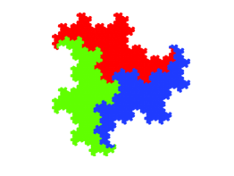
(c) Invariant sets of the GIFS.

Figure 10. A space-filling curve of Terdragon.

Example 5.1.

Terdragon. Terdragon is generated by the IFS

$$\{S_{1}(z)=\lambda z+1,\ ~{}S_{2}(z)=\lambda z+\omega,\ ~{}S_{3}(z)=\lambda z+\omega^{2}\},$$

where $\lambda=\exp(\pi{\mathbf{i}}/6)/\sqrt{3}$ and $\omega=\exp(2\pi{\mathbf{i}}/3)$. We choose the skeleton

$$A=\{a_{1},a_{2},a_{3}\}=\{-\omega^{2}/\lambda,-1/\lambda,-\omega/\lambda\},$$

which consists of the fixed points of $S_{j},j=1,2,3$. Choose the initial graph to be the cycle

$$\Lambda=\overrightarrow{a_{1}a_{2}}+\overrightarrow{a_{2}a_{3}}+\overrightarrow{a_{3}a_{1}}:=v_{1}+v_{2}+v_{3}$$

(see Figure 4(b)). The refined graph $G=S_{1}(\Lambda)\cup S_{2}(\Lambda)\cup S_{3}(\Lambda)$ is the graph in Figure 4(c). According to the of the Euler-partition in Figure 4(d), we obtain the following edge-to-trail substitution:

(5.2) $$\tau:\left\{\begin{array}[]{l}v_{1}\mapsto P_{v_{1}}=S_{1}(v_{1})+S_{2}(v_{3})+S_{2}(v_{1}),\\ v_{2}\mapsto P_{v_{2}}=S_{2}(v_{2})+S_{3}(v_{1})+S_{3}(v_{2}),\\ v_{3}\mapsto P_{v_{3}}=S_{3}(v_{3})+S_{1}(v_{2})+S_{1}(v_{3}).\end{array}\right.$$

Remark 5.2.

We shall see in Section 8 that SFCs obtained by the Euler-tour method are all closed curves, and the invariant sets of the induced GIFS form a partition of the original self-similar set $K$.

Example 5.2.

Sierpiński carpet. We choose the skeleton to be the middle points of the edges of the unit square, see Figure 3 (right). An Euler tour of the refine graph is shown in Figure 6 (b), and a partition of this Euler tour is indicated by colors. The edge-to-trail substitution is indicated by Figure 6 (a) and (d). Figure 6 (f) shows the invariants of GIFS associated with the edge-to-trail substitution, which form a partition of the carpet. (Dekking [11] gives a certain ‘parametrization’ of the carpet where there are infinitely many jumps.)

5.1. A stronger version of positive Euler tour method.

The initial cycle $\Lambda$ can be chosen to be any closed trail passing all the elements of $A$, say,

$$\Lambda=v_{1}+\cdots+v_{h}.$$

Still we can define refined graph, Euler-tour and its partition, and edge-to-trial substitution rule. In the following example, to make the visualizations self-avoid, we chooses a special closed trial $\Lambda$.

Example 5.3.

The Rocket Tile. The Rocket tile is generated by the IFS $\{S_{j}\}_{j=1}^{9}=\{(x+d)/3;{d\in D}\}$, where

$$D=\{-2,-1,-1+{\mathbf{i}},0,-{\mathbf{i}},-2{\mathbf{i}},1-{\mathbf{i}},1+{\mathbf{i}},2+2{\mathbf{i}}\}.$$

See Figure 11$(a)$. It is easy to check that $A=\{a_{1},a_{2},a_{3},a_{4}\}=\{0,-1,-{\mathbf{i}},1+{\mathbf{i}}\}$ is a skeleton. (The $a_{j}$’s are fixed points of $S_{4},S_{1},S_{6}\text{ and }S_{9}$ respectively.)

We choose the initial graph to be the closed trail

$$V=\overrightarrow{a_{1}a_{2}}+\overrightarrow{a_{2}a_{1}}+\overrightarrow{a_{1}a_{3}}+\overrightarrow{a_{3}a_{1}}+\overrightarrow{a_{1}a_{4}}+\overrightarrow{a_{4}a_{1}},$$

see Figure 11$(b)$. The refined graph of $V$ contains $54$ edges. An Euler tour of the refined graph is indicated by Figure 11$(c)$, where a partition of this tour is indicated by $6$ different colors. The edge-to-trail substitution is indicated in Figure 11$(b)$ and $(e)$.

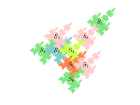
(a) Rocket.

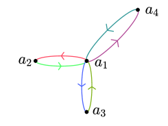
(b) Initial graph.

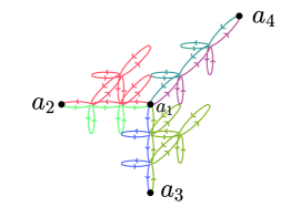
(c) Euler tour.

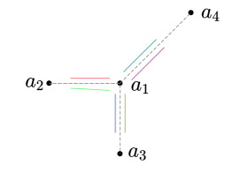
(d) Initial patterns.

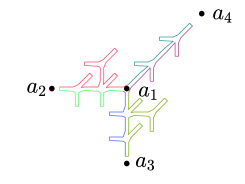
(e) The first interation.

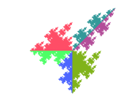
(f) Invariant sets of the GIFS.

Figure 11. A space-filling curve of the Rocket tile.

6. Linear GIFS

In this section, we recall the definition of the linear GIFS introduced in [35].

6.1. GIFS

Let $G=(\mathcal{A},\Gamma)$ be a directed graph with vertex set $\mathcal{A}$ and edge set $\Gamma$. Let

(6.1) $${\mathcal{G}}=\left(g_{\boldsymbol{\gamma}}:\mathbb{R}^{d}\rightarrow\mathbb{R}^{d}\right)_{{\boldsymbol{\gamma}}\in\Gamma}$$

be a family of similitudes. We call the triple $(\mathcal{A},\Gamma,{\mathcal{G}})$, or simply ${\mathcal{G}}$, a graph-directed iterated function system (GIFS). We call $({\mathcal{A}},\Gamma)$ the base graph of the GIFS. In what follows, we shall call ${\mathcal{A}}$ a state set instead of vertex set, to avoid confusion with other graphs. Very often but not always, we set ${\mathcal{A}}$ to be $\{1,\dots,N\}$.

Let $\Gamma_{ij}$ be the set of edges from state $i$ to $j$. It is well known that there exist unique non-empty compact sets $\{E_{i}\}_{i=1}^{N}$ satisfying

(6.2) $$E_{i}=\bigcup_{j=1}^{N}\bigcup_{{\boldsymbol{\gamma}}\in\Gamma_{ij}}g_{{\boldsymbol{\gamma}}}(E_{j}),\quad 1\leq i\leq N.$$

We call $\{E_{i}\}_{i=1}^{N}$ the invariant sets of the GIFS [26]. The set equations (6.2) provide an alternative way to define a GIFS. We shall call (6.2) the set equation form of GIFS (6.1).

6.2. Symbolic space related to a graph $G$

A sequence of edges in $G$, denoted by ${\boldsymbol{\omega}}=\omega_{1}\omega_{2}\dots\omega_{n}$, is called a walk, if the terminus of $\omega_{i}$ coincides with the origin of $\omega_{i+1}$. (Here we don’t use the notation $\omega_{1}+\cdots+\omega_{n}$ for simplicity.) We will use the following notations to for the sets of finite or infinite walks on $G=(\mathcal{A},\Gamma)$. For $i\in\mathcal{A}$, let

$$\Gamma_{i}^{k},\ \Gamma_{i}^{\ast}\text{ and }\Gamma_{i}^{\infty}$$

be the set of all walks with length $k$, the set of all walks with finite length, and the set of all infinite walks, emanating from the state $i$, respectively. Note that $\Gamma_{i}^{\ast}=\bigcup_{k\geq 1}\Gamma_{i}^{k}$.

For an infinite walk ${\boldsymbol{\omega}}=(\omega_{n})_{n=1}^{\infty}\in\Gamma_{i}^{\infty}$, we set ${\boldsymbol{\omega}}|_{k}=\omega_{1}\omega_{2}\dots\omega_{k}$ and call

$$[\omega_{1}\dots\omega_{n}]:=\{{\boldsymbol{\gamma}}\in\Gamma_{i}^{\infty};~{}~{}{\boldsymbol{\gamma}}|_{n}=\omega_{1}\dots\omega_{n}\}$$

the cylinder associated with $\omega_{1}\dots\omega_{n}$. For a walk ${\boldsymbol{\gamma}}=\gamma_{1}\dots\gamma_{n}$, we denote

$$E_{\boldsymbol{\gamma}}:=g_{\gamma_{1}}\circ\cdots\circ g_{\gamma_{n}}(E_{t({\boldsymbol{\gamma}})}),$$

where $t({\boldsymbol{\gamma}})$ denotes the terminus of the walk $\boldsymbol{\gamma}$ (and $\gamma_{n}$). Iterating (6.2) $k$-times, we obtain

(6.3) $$E_{i}=\bigcup_{{\boldsymbol{\gamma}}\in\Gamma_{i}^{k}}E_{\boldsymbol{\gamma}}.$$

We define a projection $\pi:(\Gamma_{1}^{\infty},\dots,\Gamma_{N}^{\infty})\rightarrow(\mathbb{R}^{d},\dots,\mathbb{R}^{d})$, where $\pi_{i}:\Gamma_{i}^{\infty}\rightarrow\mathbb{R}^{d}$ is defined by

(6.4) $$\{\pi_{i}({\boldsymbol{\omega}})\}:=\bigcap_{n\geq 1}E_{\boldsymbol{\omega|_{n}}}.$$

For $x\in E_{i}$, we call ${\boldsymbol{\omega}}$ a coding of $x$ if $\pi_{i}({\boldsymbol{\omega}})=x$. It is folklore that $\pi_{i}(\Gamma_{i}^{\infty})=E_{i}$.

6.3. Order GIFS and linear GIFS ([1, 35])

Let $({\mathcal{A}},\Gamma,\mathcal{G})$ be a GIFS. To study the ‘advanced’ connectivity property of the invariant sets, we equip a partial order on the edge set $\Gamma$ enlightened by set equation (6.3). Let $\Gamma_{i}=\Gamma_{i}^{1}$ be the set of edges emanating from the state $i$.

Definition 6.1.

We call the quadruple $({\mathcal{A}},\Gamma,\mathcal{G},\prec)$ an ordered GIFS, if $\prec$ is a partial order on $\Gamma$ such that

1. $\prec$ is a linear order when restricted on $\Gamma_{j}$ for every $j\in{\mathcal{A}}$;

2. elements in $\Gamma_{i}\text{ and }\Gamma_{j}$ are not comparable if $i\neq j$.

The order $\prec$ can be extend to $\Gamma_{i}^{n}$ and $\Gamma_{i}^{\infty}$ for every $i\in{\mathcal{A}}$. On $\Gamma_{i}^{n}$, two elements $\gamma_{1}\gamma_{2}\dots\gamma_{k}\prec\omega_{1}\omega_{2}\dots\omega_{k}$ if and only if $\gamma_{1}\dots\gamma_{\ell-1}=\omega_{1}\dots\omega_{\ell-1}$ and $\gamma_{\ell}\prec\omega_{\ell}$ for some $1\leq\ell\leq k$. Observe that $(\Gamma_{i}^{n},\prec)$ is a linear order. In the same manner, we can obtain a linear order of $\Gamma_{i}^{\infty}$, which we still denote by $\prec$. In the following, we say ${\boldsymbol{\omega}}$ is lower than ${\boldsymbol{\gamma}}$ if ${\boldsymbol{\omega}}\prec{\boldsymbol{\gamma}}$. Two walks ${\boldsymbol{\omega}}\prec{\boldsymbol{\gamma}}$ in $\Gamma_{i}^{n}$ are said to be adjacent if there is no walk ${\boldsymbol{\beta}}$ such that ${\boldsymbol{\omega}}\prec{\boldsymbol{\beta}}\prec{\boldsymbol{\gamma}}$.

Definition 6.2.

Let $({\mathcal{A}},\Gamma,\mathcal{G},\prec)$ be an ordered GIFS with invariant sets $\{E_{i}\}_{i=1}^{N}$. It is termed a linear GIFS, if for all $i\in{\mathcal{A}}$ and $k\geq 1$,

$$E_{\boldsymbol{\gamma}}\cap E_{\boldsymbol{\omega}}\neq\emptyset$$

provided ${\boldsymbol{\gamma}},{\boldsymbol{\omega}}$ are adjacent walks in $\Gamma_{i}^{k}$.

6.4. Chain condition

Let $(\mathcal{A},\Gamma,{\mathcal{G}},\prec)$ be an ordered GIFS. Fix $i\in\mathcal{A}$. Let ${\boldsymbol{\omega}}$ be an edge with emanating from state $i$. Let

$${\mathbf{\delta}}({\boldsymbol{\omega}})\text{ and }{\mathbf{\Delta}}({\boldsymbol{\omega}})$$

be the lowest and highest walks in $\Gamma_{i}^{\infty}$ initialled by the edge ${\boldsymbol{\omega}}$, respectively.

Definition 6.3.

An ordered GIFS is said to satisfy the chain condition, if for any $i\in{\mathcal{A}}$, and any two adjacent edges ${\boldsymbol{\omega}},{\boldsymbol{\gamma}}\in\Gamma_{i}$ with ${\boldsymbol{\omega}}\prec{\boldsymbol{\gamma}}$, it holds that

$$\pi_{i}({\mathbf{\Delta}}({\boldsymbol{\omega}}))=\pi_{i}({\mathbf{\delta}}({\boldsymbol{\gamma}})).$$

The chain condition provides a simple criterion for linear GIFS.

Theorem 6.1.

([35]) An ordered GIFS is a linear GIFS if and only if it satisfies the chain condition.

6.5. Proof of Theorem 1.3.

Let $\{S_{j}\}_{j=1}^{N}$ be a self-similar zipper with vertices $\{x_{0},\dots,x_{N}\}$ and signature $\{\beta_{1},\dots,\beta_{N}\}$. We define the following two-state GIFS:

(6.5) $$\left\{\begin{array}[]{l}E_{1}=S_{1}(E_{\beta_{1}})+\cdots+S_{N}(E_{\beta_{N}}),\\ E_{-1}=S_{N}(E_{-\beta_{N}})+\cdots+S_{1}(E_{-\beta_{1}}).\\ \end{array}\right.$$

Clearly $E_{1}=E_{-1}=K$ are the invariant sets of the above ordered GIFS, where $K$ is the invariant set of $\{S_{j}\}_{j=1}^{N}$.

Let $\pi:\{1,\dots,N\}\to K$ be the projection map associated with the IFS $\{S_{j}\}_{j=1}^{N}$. Let $\pi_{1}:\Gamma_{1}\to E_{1}$ and $\pi_{-1}:\Gamma_{-1}\to E_{-1}$ be the projections associated with $E_{1}$ and $E_{-1}$ defined as (6.4).

Let $\mathbf{\delta}$ and $\mathbf{\Delta}$ be the lowest path and highest path emanating from the state $E_{1}$, respectively. The form of $\mathbf{\delta}$ and $\mathbf{\Delta}$ are completely determined by $\beta_{1}$ and $\beta_{N}$. We claim that

$$\pi_{1}(\mathbf{\delta})=x_{0},\ \pi_{1}(\mathbf{\Delta})=x_{N}.$$

If $\beta_{1}=1$, then the lowest edge emanating from $E_{1}$ is $\omega=(E_{1},1,S_{1},E_{1})$, where the components of $\omega$ means the initial state, the order, the contraction map, and the terminal state, respectively; hence $\delta=(E_{1},1,S_{1},E_{1})^{\infty}$ and the contraction maps associated with $\delta$ is $(S_{1})^{\infty}$. On the other hand, the zipper condition implies that $S_{1}(x_{0})=x_{0}$, so we obtain

$$\pi_{1}(\delta)=\pi(1^{\infty})=x_{0}.$$

If $\beta_{N}=1$, then the highest edge emanating from $E_{1}$ is $(E_{1},N,S_{N},E_{1})$, hence $\delta=(E_{1},N,S_{N},E_{1})^{\infty}$ and the contraction maps associated with $\Delta$ is $(S_{N})^{\infty}$. On the other hand, the zipper condition implies that $S_{N}(x_{N})=x_{N}$, so we obtain

$$\pi_{1}(\Delta)=\pi(N^{\infty})=x_{N}.$$

A similar calculation as above shows that,

$$\pi_{1}(\delta)=\pi(1N^{\infty})=x_{0},\ \pi_{1}(\Delta)=\pi(N^{\infty})=x_{N}\quad\text{ if }\beta_{1}=-1,\beta_{N}=1;$$

$$\pi_{1}(\delta)=\pi(1^{\infty})=x_{0},\ \pi_{1}(\Delta)=\pi(N1^{\infty})=x_{N}\quad\text{ if }\beta_{1}=1,\beta_{N}=-1;$$

$$\pi_{1}(\delta)=\pi((1N)^{\infty})=x_{0},\ \pi_{1}(\Delta)=\pi((N1)^{\infty})=x_{N}\quad\text{ if }\beta_{1}=-1,\beta_{N}=-1.$$

Our claim is proved.

Let ${\mathbf{\delta}}^{\prime}$ and ${\mathbf{\Delta}}^{\prime}$ be the lowest path and highest path emanating from the state $E_{-1}$, respectively. Similarly, we have $\pi_{-1}({\mathbf{\delta}}^{\prime})=x_{N},\ \pi_{-1}({\mathbf{\Delta}}^{\prime})=x_{0}.$

Finally, notice that the zipper condition is exactly the chain condition, so (6.5) is a linear GIFS.

The other side is easy to prove. $\Box$

Remark 6.1.

Let $(S_{j})_{j=1}^{N}$ be an ordered IFS. One can easy calculate the four possibilities of the pair $\{x_{0},x_{N}\}$ in the above proof. Clearly $(S_{j})_{j=1}^{N}$ is a zipper if and only if there exists $(\beta_{1},\dots,\beta_{N})\in\{-1,1\}^{N}$ such that

$$S_{1}(\overrightarrow{x_{0}x_{N}}^{\beta_{1}})+\cdots+S_{N}(\overrightarrow{x_{0}x_{N}}^{\beta_{N}})$$

is a broken line.

7. Induced GIFS

In this section, we define the induced GIFS of edge-to-trail substitutions, especially we show that they are linear GIFS.

Let $\tau:u\mapsto P_{u},u\in V$ be an edge-to-trail substitution defined in Section 3. The trail $P_{u}$ can be written as

(7.1) $$P_{u}=S_{u,1}(v_{u,1})+\dots+S_{u,\ell_{u}}(v_{u,\ell_{u}}),$$

where $S_{u,j}\in\mathcal{S}$ and $v_{u,j}\in V$ for $j=1,\dots,\ell_{u}$.

According to $\tau$ we can construct an ordered GIFS as follows. Replacing $P_{u}$ by $E_{u}$ on the left hand side, and replacing $v$ by $E_{v}$ on the right hand side of (7.1), we obtain an ordered GIFS:

(7.2) $$E_{u}=S_{u,1}(E_{v_{u,1}})+\cdots+S_{u,\ell_{u}}(E_{v_{u,\ell_{u}}}),\quad u\in V,$$

which we the induced GIFS of $\tau$. In an ordered GIFS, we use $``+"$ to replace the $``\cup"$ in the set equation to emphasis the order structure.

Example 7.1.

Induced GIFS of Terdragon. The edge-to-trail substitution $\tau$ in Example 5.1 induces the following GIFS:

$$\left\{\begin{array}[]{l}E_{1}=S_{1}(E_{1})+S_{2}(E_{3})+S_{2}(E_{1}),\\ E_{2}=S_{2}(E_{2})+S_{3}(E_{1})+S_{3}(E_{2}),\\ E_{3}=S_{3}(E_{3})+S_{1}(E_{2})+S_{1}(E_{3}).\end{array}\right.$$

The invariant sets $E_{j}$ are illustrated in Figure 10(c).

Let

(7.3) $$(V,\Gamma,\mathcal{G},\prec)$$

be the basic-graph form of the ordered GIFS (7.2). The state set is $V$, which is the edges of the initial graph. The edge set $\Gamma$ consists of quadruples $(u,S_{j},v,k)$, that is, if $S_{j}(v)$ is the $k$-th edge in the trail $P_{u}$, then we add an edge to $\Gamma$ and denote this edge by

(7.4) $$(u,S_{j},v,k)\in\Gamma.$$

The contraction associated with this edge is $S_{j}$.

Theorem 7.1.

The induced GIFS (7.2) is a linear GIFS.

Proof.

Let $u\in V$. We denote by $a_{u}$ and $b_{u}$ the origin and the terminus of $u$ as an edge in the initial graph $\Lambda=(A,V)$. We claim that the lowest and highest elements in $\Gamma_{u}^{\infty}$ are codings of $a_{u}$ and $b_{u}$, respectively.

Let $S(v)$ be the first edge in $P_{u}$, then $\omega=(u,S,v,1)$ is the lowest edge emanating from $u$ in the basic graph $\Gamma$. It follows that

(7.5) $$a_{u}=S(a_{v}).$$

Therefore, if $(\omega_{n})_{n=1}^{\infty}$ is a coding of $a_{v}$, then

$$\omega(\omega_{n})_{n-1}^{\infty}$$

is a coding of $a_{u}$. Applying the same argument to $v$, we obtain a coding of $a_{u}$, such that the first two edges of this coding is the lowest walk in $\Gamma_{u}^{2}$. Continuing this argument, we conclude the lowest element in $\Gamma_{u}^{\infty}$ is a coding of $a_{u}$.

Similarly, the highest element in $\Gamma_{u}^{\infty}$ is a coding of $b_{u}$.

Now, let $\omega=(u,S,v,k)$ and $\gamma=(u,T,v^{\prime},k+1)$ be two consecutive edges in $\Gamma_{u}$. This means that $S(v)$ and $T(v^{\prime})$ are two adjacent edges in $P_{u}$, so $S(b_{v})=T(a_{v^{\prime}})$.

On the other hand, write $\Delta(\omega)=\omega(\omega_{n})_{n\geq 1}$, then $(\omega_{n})_{n\geq 1}$ is the highest coding in $\Gamma_{v}$. So $\pi_{v}((\omega_{n})_{n\geq q})=b_{v}$ by the claim above, and

$$\pi_{u}(\Delta(\omega))=S\circ\pi_{v}((\omega_{n})_{n\geq q})=S(b_{v}).$$

Similarly, we have $\pi_{u}(\delta(\gamma))=T(a_{v^{\prime}})$. This verifies the chain condition. Therefore, the ordered IFS in consideration is linear. ∎

Proof of Theorem 1.2. Let $\tau$ be an edge-to-trail substitution over $V$ such that $\tau(u)$ are all traveling trails. Let us denote the induced GIFS of $\tau$ by $(V,\Gamma,{\mathcal{G}},\prec)$. Let $g_{\omega}$ be the contraction associated with the edge $\omega$ in $\Gamma$.

Fix an $u\in V$. The traveling property of $\tau$ implies that the associated contractions with edges in $\Gamma_{u}^{n}$ are exactly the maps $S_{I},{I\in\{1,\dots,N\}^{n}}$, and each maps appears only once. It follows that

$$\bigcup_{{\boldsymbol{\omega}}\in\Gamma_{u}^{n}}g_{{\boldsymbol{\omega}}}(\{0\})=\bigcup_{I\in\{1,\dots,N\}^{n}}S_{I}(\{0\}),$$

where $g_{\boldsymbol{\omega}}=g_{\omega_{1}}\circ\cdots\circ g_{\omega_{n}}$ is the contraction associated to the trail ${\boldsymbol{\omega}}$. Taking the limit in Hausdorff metric at both sides, we obtain $E_{u}=K$. This proves that the invariant sets of the GIFS are all equal to $K$.

Moveover, if we ignor the order structure, then the induced GIFS degenerates to the original IFS of $K$, so the induced GIFS satisfies the OSC. Hence, $K$ admits optimal parameterizations according to Theorem 1.1. $\Box$

8. (General) Euler-tour method

In this section, we introduce the general Euler-tour method. Recall that $A=\{a_{1},\dots,a_{m}\}$ is a skeleton, and $\Lambda=(A,V^{+})$ is the cycle passing all elements of $A$, see Section 5. For simplicity, we denote

$$v_{j}=\overrightarrow{a_{j}a_{j+1}}\text{ and }v_{j}^{-1}=\overrightarrow{a_{j+1}a_{j}},\quad j=1,\dots,m,$$

where we identify $a_{m+1}$ with $a_{1}$. Then $\Lambda=v_{1}+v_{2}+\cdots+v_{m},$ and we denote $\Lambda^{-1}=v_{m}^{-1}+\cdots+v_{1}^{-1}$ to be the reverse of $\Lambda$.

Let $\beta=(\beta_{1},\beta_{2},\cdots,\beta_{N})\in\{1,-1\}^{N}$, and we call it an orientation vector. Denote

(8.1) $$G(\mathcal{S},A,\beta)=\bigcup_{j=1}^{N}S_{j}(\Lambda^{\beta_{j}}).$$

By the same argument as Lemma 5.1, one can show that $G(\mathcal{S},A,\beta)$ admits Euler tour.

Definition 8.1.

Let $P$ be an Euler tour of $G({\mathcal{S}},A,\beta)$, and let

$$P=P_{1}+\cdots+P_{m}$$

be a partition of $P$. We call it an Euler-partition of $G({\mathcal{S}},A_{\tau},\beta)$ if the initial points of $P_{1},\dots,P_{m}$, denoted by $a_{\tau^{\prime}(1)},\dots,a_{\tau^{\prime}(m)}$, is a permutation of $A$. We call $\tau^{\prime}$ the output permutation of $P_{1}+\cdots+P_{m}$.

(a) $P=P_{1}+P_{2}+P_{3}$

(b) $P^{-1}=P_{3}^{-1}+P_{2}^{-1}+P_{3}^{-1}$

(c) $P^{2}=P\circ P$

Figure 12. $G(\mathcal{S},A,\beta)$ and $G(\mathcal{S},A,-\beta)$.

8.1. Consistency and induced edge-to-trail substitution

Definition 8.2.

We say an Euler-partition $P_{1}+\cdots+P_{m}$ of $G(\mathcal{S},A,\beta)$ is consistent, if $P_{i}$ has the same origin and terminus as $v_{i}$ for each $i\in\{1,2,\dots,h\}$, or equivalently, its output permutation is the identity.

As soon as $P_{1}+\cdots+P_{m}$ is consistent, we can define an edge-to-trail substitution over

$$V=V^{+}\cup V^{-}=\{v_{1},\dots,v_{m}\}\cup\{v_{1}^{-1},\dots,v_{m}^{-1}\}$$

as

(8.2) $$\tau:v_{j}\mapsto P_{j}\text{ and }v_{j}^{-1}\mapsto P_{j}^{-1},\quad j=1,\dots,m.$$

We call $\tau$ the induced edge-to-trail substitution of the Euler-partition $P_{1}+\cdots+P_{m}$.

Remark 8.1.

Set $G=\bigcup_{i=1}^{N}S_{i}(\Lambda\cup\Lambda^{-1})=G(\mathcal{S},A,\beta)\cup G(\mathcal{S},A,-\beta)$, and we see that the generalized Euler-tour method is a special case of the construction in Section 3.

Denote the length of $P_{j}$ by $\ell_{j}$, then $P_{j}$ has the form

(8.3) $$P_{j}=S_{j,1}(u_{j,1})+S_{j,2}(u_{j,2})+\cdots+S_{j,\ell_{j}}(u_{j,\ell_{j}}),\quad j=1,\dots,m.$$

where $S_{j,k}\in\{S_{1},\dots,S_{N}\}$, and $u_{j,k}\in V$. Accordingly,

(8.4) $$P_{j}^{-1}=S_{j,\ell_{j}}(u^{-1}_{j,\ell_{j}})+\cdots+S_{j,2}(u^{-1}_{j,2})+S_{j,1}(u^{-1}_{j,1}),\quad j=1,\dots,m.$$

The substitution (8.2) induces the following linear GIFS (by Theorem 7.1 ):

(8.5) $$\left\{\begin{array}[]{c}E_{v_{j}}=S_{j,1}(E_{u_{j,1}})+S_{j,2}(E_{u_{j,2}})+\cdots+S_{j,\ell_{j}}(E_{u_{j,\ell_{j}}}),\\ E_{v_{j}^{-1}}=S_{j,\ell_{j}}(E_{u^{-1}_{j,\ell_{j}}})+\cdots+S_{j,2}(E_{u^{-1}_{j,2}})+S_{j,1}(E_{u^{-1}_{j,1}}).\end{array}\right.\quad 1\leq j\leq m.$$

For simplicity, we call GIFS (8.5) the induced GIFS of the Euler-partition $P_{1}+\cdots+P_{m}$. We shall use $(V,{\mathcal{E}},{\mathcal{G}},\prec)$ to denote this GIFS, as we explained in Section 7.

Now we give some basic properties of the induced GIFS.

Lemma 8.2.

(i) $E_{v}=E_{v^{-1}}$ for $v\in V$.

(ii) For each $v\in V$ and $i\in\{1,\dots,N\}$, $S_{i}(E_{v})$ appears exactly once in the right-hand side of (8.5).

(iii) $K=\bigcup_{v\in V^{+}}E_{v}$.

Proof.

(i) Set $F_{v}=E_{v^{-1}}$ for $v\in V$. Clearly $\{F_{v}\}_{v\in V}$ also satisfy the set equation (8.5) if we ignore the order structure. Hence (i) follows from the uniqueness of the invariant sets.

(ii) Since $P$ is an Euler tour, for each $v\in V$ and $i\in\{1,\dots,N\}$, the edge $S_{i}(v)$ appears exactly once in $P\cup P^{-1}$, which implies (ii).

(iii) Taking the union of both sides of (8.5) and using the conclusion of (ii), we have

(8.6) $$\bigcup_{v\in V}E_{v}=\bigcup_{j=1}^{m}\bigcup_{k=1}^{l_{j}}S_{j,k}(E_{u_{j,k}}\cup E_{u_{j,k}^{-1}})=\bigcup_{i=1}^{N}S_{i}(\cup_{v\in V}E_{v}).$$

Therefore, by the uniqueness of the invariant set of an IFS, we obtain

$$K=\bigcup_{v\in V}E_{v}=\bigcup_{v\in V^{+}}E_{v},$$

where the last equality holds since $E_{v}=E_{v^{-1}}$. ∎

Lemma 8.2 (ii) means that for each $v\in V$, there are exactly $N$ edges in $\Gamma$ terminating at $v$; moreover, the associated maps of these edges run over the maps $S_{1},\dots,S_{N}$.

8.2. Primitivity and the open set condition

To ensure the induced GIFS satisfies the OSC, we need a primitivity condition.

Since $E_{v}=E_{v^{-1}}$, in the induced GIFS, we can identify $E_{v}$ and $E_{v^{-1}}$ to simplify the discussion. By identifying $v$ and $v^{-1}$ in $\tau$, and ignoring the maps $S_{j}$ in $\tau(v)$, we define a morphism over $\{v_{1},\dots,v_{m}\}$ by

(8.7) $$\tau^{*}:~{}~{}v_{j}\longrightarrow|v_{j,1}|~{}|v_{j,2}|~{}\dots~{}|v_{j,l_{j}}|,\quad j=1,2,\dots,m,$$

where $|v|=|v^{-1}|=v$ for $v\in V^{+}$. We call $\tau^{*}$ the induced morphism. Recall that $\tau^{*}$ is primitive if there exists an integer $n$ such that for any $i,j\in\{1,2,\dots,m\}$, $v_{i}$ appears in $(\tau^{*})^{n}(v_{j})$; see for instance [33].

Definition 8.3.

We say a consistent Euler-partition $P_{1}+\cdots+P_{m}$ of $G({\mathcal{S}},A,\beta)$ is primitive, if the induced morphism $\tau^{*}$ is primitive.

Example 8.1.

Consider the Sierpiński gasket. Let $\beta=(1,-1,-1)$. Figure 12(a) illustrates a consistent partition $P_{1}+P_{2}+P_{3}$ , where the trails are indicated by colors. The induced edge-to-trail substitution is:

(8.8) $$\tau:\left\{\begin{array}[]{l}v_{1}\mapsto P_{1}=S_{1}(v_{1})+S_{2}(v_{3}^{-1})+S_{2}(v_{2}^{-1}),\\ v_{2}\mapsto P_{2}=S_{2}(v_{1}^{-1})+S_{1}(v_{2})+S_{3}(v_{3}^{-1}),\\ v_{3}\mapsto P_{3}=S_{3}(v_{2}^{-1})+S_{3}(v_{1}^{-1})+S_{1}(v_{3}).\\ \end{array}\right.$$

The induced morphism is

$$\tau^{*}:\left\{\begin{array}[]{cl}v_{1}&\mapsto v_{1}v_{3}v_{2},\\ v_{2}&\mapsto v_{1}v_{2}v_{3},\\ v_{3}&\mapsto v_{2}v_{1}v_{3}\end{array}\right.$$

and it is primitive. Figure 12 illustrates $\tau^{3}(\Lambda)$.

For a GIFS $(V,\Gamma,{\mathcal{F}})$, let $r_{e}$ be the contraction ratio of the mapping associated with the edge $e$. For $s>0$, the Mauldin-Williams matrix $M(s)$ is defined to be ([26])

(8.9) $$\left(\begin{array}[]{c}\sum_{e\in\Gamma_{uv}}r_{e}^{s}\\ \end{array}\right)_{u,v\in V}.$$

The real number $s$ satisfying $\Phi(M(s))=1$ is called the similarity dimension of the GIFS, where $\Phi(\cdot)$ denotes the spectral radius of a matrix.

Let ${\mathcal{H}}^{s}$ be the $s$-dimensional Hausdorff measure; a set $E$ is called an $s$-set, if $0<{\mathcal{H}}^{s}(E)<\infty$. A directed graph is said to be strongly connected, if for any pair of vertice $i$ and $j$, there is trail from $i$ to $j$. The following criterion of the OSC is proved in [26] (the ‘only if’ part) and [23] (the ‘if’ part).

Lemma 8.3.

Let ${\mathcal{F}}$ be a GIFS with a strongly connected base graph. Denote its invariant sets by $\{E_{j}\}_{j=1}^{N}$, and the self-similar dimension by $\delta$. Then ${\mathcal{F}}$ satisfies the open set condition if and only if

$$0<{\mathcal{H}}^{\delta}(E_{j})<+\infty$$

for some $1\leq j\leq N$ (or for all $1\leq j\leq N$).

Theorem 8.1.

Let $P_{1}+\cdots+P_{m}$ be a consistent and primitive Euler-partition of $G(S,A,\beta)$. Then the induced GIFS (8.5) satisfies the OSC, and

$$0<{\mathcal{H}}^{s}(E_{v})<\infty,\text{ for all }v\in V,$$

where $s=dim_{H}K$.

Proof.

First, we show that the similarity dimension of the induced GIFS is $s=\dim_{H}K$. Let $c_{j}$ be the contraction ratio of $S_{j}$. Then $s$ fulfills the equation $\sum_{j=1}^{N}c_{j}^{s}=1$ and $0<{\mathcal{H}}^{s}(K)<\infty$, since ${\mathcal{S}}$ satisfies the OSC. Recall that

(8.10) $$M(s)=\left(\begin{array}[]{c}\sum_{e\in\Gamma_{uv}}r_{e}^{s}\\ \end{array}\right)_{u,v\in V}.$$

By Lemma 8.2(ii), we have (since $\cup_{u\in V}\Gamma_{uv}$ is the set of edges with terminus $v$)

$$\sum_{u\in V}\sum_{e\in\Gamma_{uv}}r_{e}^{s}=\sum_{i=1}^{N}c_{i}^{s}=1,\quad v\in V,$$

namely, the sum of entries of each collum of $M(s)$ is $1$. By Perron-Frobenius Theorem (see Lemma 8.4 below), the spectral radius of $M(s)$ equals $1$, which implies that $s$ is the similarity dimension of the induced GIFS.

We identify $E_{v}$ and $E_{v^{-1}}$ in the induced GIFS (8.5) and forget the order, then we obtain a simplified GIFS as follows:

(8.11) $$E_{v_{j}}=S_{j,1}(E_{|u_{j,1}|})\cup S_{j,2}(E_{|u_{j,2}|})\cup\cdots\cup S_{j,\ell_{j}}(E_{|u_{j,\ell_{j}}|}),\quad j=1,\dots,m.$$

We have the following facts concerning the simplified GIFS:

$(i)$ The base graph of the simplified GIFS is strongly connected, since the induced morphism $\tau^{*}$ is primitive.

$(ii)$ The relation $\mathcal{H}^{s}(E_{v_{j}})>0$ holds for at least one $j$, since the union $K=\bigcup_{j=1}^{m}E_{v_{j}}$ is has a finite and positive $s$-dimensional Hausdorff measure.

$(iii)$ The simplified GIFS has the same similarity dimension as the induced GIFS, which is $s$. This is true because the sum of each row of the associated matrix $\tilde{M}(s)$ of the simplified GIFS is still $1$, where

$$\tilde{M}(s)=\left(\begin{array}[]{c}\sum_{e\in\Gamma_{uv}}r_{e}^{s}+\sum_{e\in\Gamma_{uv^{-1}}}r_{e}^{s}\\ \end{array}\right)_{u,v\in V^{+}}.$$

Item (i)-(iii) verify the conditions of Lemma 8.3, hence the simplified GIFS satisfies the OSC, which implies $0<{\mathcal{H}}^{s}(E_{v})<\infty$ for all $v\in V^{+}$ (again by Lemma 8.3).

Finally, we observe that if the simplified GIFS satisfies the OSC with open sets $U_{1},\dots,U_{m}$, then the induced GIFS satisfies the OSC with the open sets $U_{1},\dots,U_{m},U_{1},\dots,U_{m}$. ∎

The following is a part of the Perron-Frobenius Theorem, see for example [29].

Lemma 8.4.

(Perron-Frobenius Theorem) Let $B=[a_{ij}]$ be a non-negative $k\times k$ matrix.

(i) There is a non-negative eigenvalue $\lambda$ such that it is the spectral radius $B$.

(ii) We have $\displaystyle\min_{i}\left(\sum_{j=1}^{k}a_{ij}\right)\leq\lambda\leq\max_{i}\left(\sum_{j=1}^{k}a_{ij}\right)$.

8.3. Pure-cell property and the disjointness of $K=\bigcup_{v\in V^{+}}E_{v}$

Finally, we investigate when $K=\bigcup_{v\in V^{+}}E_{v}$ is a disjoint union in Hausdorff measure. For $I\in\Sigma^{n}$, we call the set of edges

$$\{S_{I}(v);v\in V\}\text{ and }\{S_{I}(v);v\in V^{-1}\})$$

a positive and a negative $S_{I}$-cell, respectively.

Definition 8.4.

Let $\tau$ be an edge-to-trail substitution induced by an Euler-partition $P_{1}+\cdots+P_{m}$. Let $I\subset\Sigma^{n}$. The cell $S_{I}(\Lambda^{\pm 1})$ is called a pure cell, if there exists $u\in V$ such that the $S_{I}$-cell is a subgraph of $\tau^{n}(u)$. In this case, we also say the partition $P_{1}+\cdots+P_{m}$ potentially contains pure cell.

Theorem 8.2.

Let ${\mathcal{S}}=\{S_{i}\}_{1\leq i\leq N}$ be an IFS satisfying the OSC, and let $A$ be a skeleton of ${\mathcal{S}}$. If there exist a vector $\beta\in\{-1,1\}^{N}$ and an Euler-partition $P_{1}+\cdots+P_{m}$ of $G({\mathcal{S}},A,\beta)$ such that the partition is consistent, primitive and potentially contains pure cells, then

(i) $K=\bigcup_{v\in V^{+}}E_{v}$ is a disjoint union in the $s$-dimensional Hausdorff measure, where $s=\dim_{H}K$;

(ii) the edge-to-trail substitution $\tau$ in (8.2) leads to a a space-filling curve of $K$.

Proof.

(i) Suppose that an $S_{I}$-cell is a pure cell, i.e., all the edges of the $S_{I}$-cell belong to $\tau^{n}(u)$ for some $u\in V$, where $n=|I|$. Without loss of generality, we may assume that the orientation of the $S_{I}$-cell is positive. Then all $S_{I}(E_{v}),v\in V^{+}$ appear in the right hand side of the $n$-th iteration of the set equation (8.5) corresponding to $E_{u}$. Hence, $\bigcup_{v\in V^{+}}S_{I}(E_{v})$ is a disjoint union in the $s$-dimensional Hausdorff measure, since the induced GIFS satisfies the OSC (by Theorem 8.1); it follows that its image under $S_{I}^{-1}$, $\bigcup_{v\in V^{+}}E_{v}$ is also a disjoint union in Hausdorff measure.

(ii) By Theorem 7.1, the induced GIFS is a linear GIFS. By Theorem 8.1, the induced GIFS satisfies the OSC, and all the invariant sets are $s$-sets.

Let $L_{j}={\mathcal{H}}^{s}(E_{v_{j}})$, and $L=\sum_{j=1}^{m}L_{j}$. By Theorem 1.1, for each $j\in\{1,\dots,m\}$, there exists an optimal parametrization $\varphi_{j}:[0,L_{j}]\mapsto E_{v_{j}}$ such that $\varphi_{j}(0)$ and $\varphi_{j}(L_{j})$ are the origins and terminus of $v_{j}$, respectively.

Let $\varphi:[0,L]\to K$ be the curve obtained by joining all the $\varphi_{i}$ one by one. Since $K=\bigcup_{v\in V^{+}}E_{v}$ is a disjoint union in measure, we conclude that $\varphi$ is an optimal parametrization of $K$. ∎

(a) Initial trail: positive

(b) Initial trail: negative

(c) Euler tour

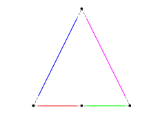
(d) Initial pattern

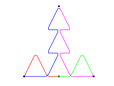
(e) First generation

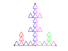
(f) Second generation

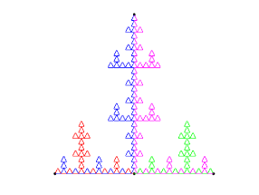
(g) Third generation

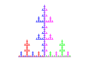
(h) Invariant sets of the linear GIFS

Figure 13. Christmas tree

8.4. The Christmas tree

The Christmas tree is the invariant set of the IFS $\{S_{j}\}_{j=1}^{5}=\{(x+d)/3;d\in D\}$, where $D=\{0,1,2,1+{\mathbf{i}},1+2{\mathbf{i}}\}$. We choose $A=\{a_{1},a_{2},a_{3},a_{4}\}=\{0,1/2,1,1/2+i\}$, which are the fixed points of $S_{1},S_{2},S_{3},S_{5}$. Let $v_{i}=\overrightarrow{a_{i}a_{i+1}}$ (assume $a_{5}=a_{1}$) and let $\Lambda=v_{1}+v_{2}+v_{3}+v_{4}.$

To get a primitive substitution, we choose an orientation vector $\beta=(-1,1,-1,1,1)$. Using the Euler-partition in Figure 13 (e), we get the following edge-to-trail substitution

(8.12) $$\left\{\begin{array}[]{l}v_{1}\mapsto S_{1}(v_{4}^{-1})+S_{1}(v_{3}^{-1})+S_{2}(v_{1}),\\ v_{2}\mapsto S_{2}(v_{2})+S_{3}(v_{4}^{-1})+S_{3}(v_{3}^{-1}),\\ v_{3}\mapsto S_{3}(v_{2}^{-1})+S_{3}(v_{1}^{-1})+S_{2}(v_{3})+S_{4}(v_{2})+S_{4}(v_{3})+S_{5}(v_{2})+S_{5}(v_{3}),\\ v_{4}\mapsto S_{5}(v_{4})+S_{5}(v_{1})+S_{4}(v_{4})+S_{4}(v_{1})+S_{2}(v_{4})+S_{1}(v_{2}^{-1})+S_{1}(v_{1}^{-1}).\end{array}\right.$$

and the rules for $v_{1}^{-1},v_{2}^{-1},v_{3}^{-1},v_{4}^{-1}$ can be obtained accordingly.

9. Consistency

In this section and next section, we will confirm the conditions in Theorem 8.2. In this section, we study the existence of consistent Euler-partitions.

Let $\mathcal{S}=\{S_{j}\}_{j=1}^{N}$ be an IFS possessing a skeleton $A=\{a_{1},a_{2},\dots,a_{m}\}$. Let $K$ be the invariant set of ${\mathcal{S}}$. Recall that $\Sigma=\{1,\dots,N\}.$

Let $\tau$ be a permutation of $\{1,\dots,m\}$. Let $\Lambda_{\tau}$ be the cycle passing the elements of $A_{\tau}=\{a_{\tau(1)},\dots,a_{\tau(m)}\}$ one by one. As before, we define

(9.1) $$G({\mathcal{S}},A_{\tau},\beta)=\bigcup_{j\in\Sigma}S_{j}(\Lambda_{\tau}^{\beta_{i}}).$$

For simplicity, we abbreviate $G(\mathcal{S},A_{\tau},\beta)$ as $G({\mathcal{S}},A_{\tau})$ when $\beta=(1,1,\dots,1)$ is totally positive. The main idea in this section is to generate an Euler tour of $G({\mathcal{S}},A_{\tau})$ by a bubbling process.

9.1. Bubbling property

First, we give some definitions. We say two subgraphs $H_{1}$ and $H_{2}$ are disjoint, denoted by $H_{1}\cap H_{2}=\emptyset$, if they do not have a common edge.

Let $P$ be an Euler tour of a directed graph $G$, and let $C=e_{1}+\cdots+e_{h}\subset G$ be a cycle. We call $C$ a remaining cycle of $P$, if $e_{j}$ appears earlier than $e_{j+1}$ in $P$ for all $1\leq j<h$ when we regard $e_{1}$ as the starting edge of $P$. In this case, $P$ can be uniquely written as

(9.2) $$P=e_{1}+L_{1}+\cdots+e_{h}+L_{h},$$

where some $L_{j}$ may be empty trails. We call $L_{j}$ out-trails w.r.t. $C$, and call (9.2) the out-trail decomposition of $P$ w.r.t. $C$.

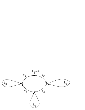
Figure 14. A remaining cycle $C=e_{1}+e_{2}+e_{3}+e_{4}$ and its out-trials.

Definition 9.1.

(Cell-exact subgraph.) A subgraph $H$ of $G({\mathcal{S}},A_{\tau})$ is said to be cell-exact, if for all cell $S_{k}(\Lambda_{\tau})$, either $S_{k}(\Lambda_{\tau})\subset H$ or $S_{k}(\Lambda_{\tau})\cap H=\emptyset$.

Definition 9.2.

(Bubbling property.) Let $H\subset G(\mathcal{S},A_{\tau},\beta)$ be a cell-exact subgraph, and let $P$ be an Euler tour of $H$. We say $P$ satisfies the bubbling property, if for all $S_{i}(\Lambda)\subset H$, the cell $S_{i}(\Lambda)$ is a remaining cycle of $P$, and all the outpaths w.r.t. $S_{i}(\Lambda)$ are cell-exact.

The goal of this section is to prove the following theorem.

Theorem 9.1.

There exist an integer $n$ and a permutation $\tau$ such that $G(\mathcal{S}^{n},A_{\tau})$ has an Euler-partition $P=P_{1}+\cdots+P_{m}$ which is consistent and satisfies the bubbling property.

Definition 9.3.

Let $P$ be an Euler tour of $G({\mathcal{S}},A_{\tau},\beta)$. We say a cell $S_{i}(\Lambda_{\tau})$ is unbroken, if $S_{i}(\Lambda_{\tau})=e_{1}+\cdots+e_{m}$ is a subtrail of $P$. (Here $e_{1}$ can be any edge in $S_{i}(\Lambda_{\tau})$.)

9.2. Bubbling process

Recall that $H(\mathcal{S},A)$ is the Hata graph induced by $A$, see Definition 2.1. It is a connected undirected graph.

A subgraph $R$ of $H(\mathcal{S},A)$ is called a spanning tree, if $R$ is a tree containing A. (Recall that an undirected connected graph is called a tree, if it does not contain cycles.) A vertex $v$ of a tree $R$ is called a top, if $v$ is a vertex of degree one.

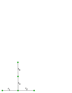
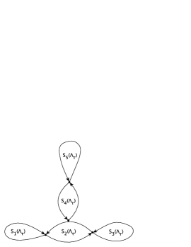
Figure 15. A spanning tree and bubbling process.

From now on, we choose a spanning tree $R$ of $H({\mathcal{S}},A)$ and fix it. We choose an order of the edges of $R$, say,

(9.3) $$r_{1},\dots,r_{N-1},$$

such that for any $1\leq j\leq N-1$, the subgraph consisting of the edges $r_{1},\dots,r_{j}$ is connected. This means that starting from a certain cell, we can add the cells one by one following above order to obtain $G(S,A_{\tau})$, and all the subgraphs in the process are connected. By changing the name of $S_{j}$, we may assume without loss of generality that the cells are added in the order $S_{1}(\Lambda_{\tau}),\dots,S_{N}(\Lambda_{\tau})$. Then one vertex of $r_{j}$ is $S_{j+1}$, and the other vertex of $r_{j}$ belongs to $\{S_{1},S_{2},\dots,S_{j}\}$, which we denote by $S_{\varphi(j)}$. We note that if $S_{k}$ is a top of $R$, then $\varphi(j)\neq k$ for any $j$. See Figure 15.

Now, we construct inductively a sequence $(\Delta_{k})_{k=1}^{N}$ such that $\Delta_{k}$ is an Euler tour of $\bigcup_{j=1}^{k}S_{j}(\Lambda_{\tau})$ satisfying the bubbling property in Definition 9.2.

Let $\Delta_{1}=S_{1}(\Lambda_{\tau})$ be the first Euler tour, which clearly satisfies the bubbling property.

Suppose $\Delta_{k}$ has been constructed, $1\leq k\leq N-1$. Now we add the cell $S_{k+1}(\Lambda_{\tau})$ to $\Delta_{k}$. In the spanning tree $R$, $S_{k+1}$ is connected to $S_{\varphi(k)}\in\{S_{1},\dots,S_{{k}}\}$, so

$$S_{k+1}(A)\cap S_{\varphi(k)}(A)\neq\emptyset.$$

Take any point $z^{*}$ from the above intersection. Write

$$S_{\varphi(k)}(\Lambda_{\tau})=e_{1}+\cdots+e_{m}\text{ and }S_{k+1}(\Lambda_{\tau})=e_{1}^{\prime}+\cdots+e_{m}^{\prime},$$

where both $e_{1}$ and $e_{1}^{\prime}$ have origin $z^{*}$. The outpath decomposition of $\Delta_{k}$ w.r.t. $S_{\varphi(k)}(\Lambda_{\tau})$ can be written as $\Delta_{k}=e_{1}+L_{1}+\cdots+e_{m}+L_{m}.$ Set

$$\Delta_{k+1}=e_{1}+L_{1}+\cdots+e_{m}+L_{m}+(e_{1}^{\prime}+\cdots+e_{m}^{\prime}).$$

Clearly, $\Delta_{k+1}$ is an Euler tour of the graph $\bigcup_{j=1}^{k+1}S_{j}(\Lambda_{\tau}).$

Now we show that $\Delta_{k+1}$ satisfies the bubbling property. For a cell $S_{j}(\Lambda_{\tau})\subset\Delta_{k+1}$, no matter it is $S_{k+1}(\Lambda_{\tau})$, or is $S_{\varphi(k)}(\Lambda_{\tau})$, or belongs to a certain $L_{i}(1\leq i\leq k)$, one can easily prove that it is a remaining cycle of $\Delta_{k+1}$ and all its out-trials are cell-exact. The bubbling property is proved.

Set $k=N$, we obtain the following:

Lemma 9.1.

For any permutation $\tau$ of $A$, there exists an Euler tour $\Delta$ of $G({\mathcal{S}},A_{\tau})$ satisfying the bubbling property. Moreover, if $S_{i}$ is a top of the spanning tree $R$, then $S_{i}(\Lambda_{\tau})$ is an unbroken cell of $\Delta$.

9.3. A natural Euler-parition of $\Delta$.

Now we introduce a natural partition of $\Delta$. We start from the vertex $a_{1}$, and walk along $\Delta$. We record the elements of $A$ appearing on the Euler tour but without repetition, then we get a rearrangement of $A$, which we denote by

$$a_{\tau^{*}(1)},\cdots,a_{\tau^{*}(m)}.$$

Let $P_{j}$ be the subtrail of $\Delta$ starting from the first visiting of $a_{\tau^{*}(j)}$ and ending at the first visiting of $a_{\tau^{*}(j+1)}$, then

$$P_{1}+\cdots+P_{m}$$

is an Euler-partition of $G({\mathcal{S}},A_{\tau})$ with output permutation $\tau^{*}$, which we denoted by ${\mathcal{P}}_{\tau}$.

9.4. A cycle of permutations of $A$

Starting from a permutation $\tau$ of $A$, we can construct an Euler-partition ${\mathcal{P}}_{\tau}$ of $G(S,A_{\tau})$, and we denote its output permutation by $\tau^{*}$. Since there are only finite many permutations of $A$, there exist $\tau_{1},\dots,\tau_{h}$ such that $\tau_{j+1}$ is the output permutation of ${\mathcal{P}}_{\tau_{j}}$, $1\leq j\leq h-1$, and $\tau_{1}$ is the output permutation of ${\mathcal{P}}_{\tau_{h}}$.

9.5. Composition of Euler-partition

Let $P=P_{1}+\cdots+P_{m}$ be an Euler-partition of $G({\mathcal{S}},A_{\tau_{1}})$ with output permutation $\tau_{2}$, and let $Q=Q_{1}+\cdots+Q_{m}$ be an Euler-partition of $G({\mathcal{S}}^{n},A_{\tau_{2}})$ with output permutation $\tau_{3}$. Since $Q$ is an Euler tour of

$$\bigcup_{I\in\Sigma^{n}}S_{I}(\Lambda_{\tau_{2}}),$$

each edge in $Q$ can be written as

(9.4) $$S_{I}(\overrightarrow{a_{\tau_{2}(k)}a_{\tau_{2}(k+1)}}).$$

Notice that $S_{I}(P_{k})$ is a trail having the same origin and terminus as the edge in (9.4). So, we can define an Euler tour of $G(S^{n+1},A_{\tau_{1}})$ by replacing every edge $S_{I}(\overrightarrow{a_{\tau_{2}(k)}a_{\tau_{2}(k+1)}})$ in $Q$ by the trail $S_{I}(P_{k})$.

We denote this replacement rule by $\sigma$, that is,

(9.5) $$\sigma(S_{I}(\overrightarrow{a_{\tau_{2}(k)}a_{\tau_{2}(k+1)}}))=S_{I}(P_{k}),\quad I\in\{1,\dots,N\}^{n},\ k\in\{1,\dots,m\},$$

and set $\sigma({\boldsymbol{\omega}})=\sigma(\omega_{1})+\dots+\sigma(\omega_{\ell})$ for any trail ${\boldsymbol{\omega}}=\omega_{1}+\dots+\omega_{\ell}$. We define the composition of $P$ and $Q$ to be

$$Q\circ P=\sigma(Q_{1})+\cdots\sigma(Q_{m}),$$

which is an Euler-partition of $G(\mathcal{S}^{n+1},A_{\tau_{1}})$.

Lemma 9.2.

Let $P=P_{1}+\cdots+P_{m}$ be an Euler-partition of $G(S,A_{\tau_{1}})$ with output permutation $\tau_{2}$, and let $Q=Q_{1}+\cdots+Q_{m}$ be an Euler-partition of $G(S^{n},A_{\tau_{2}})$ with output permutation $\tau_{3}$. Then

(i) If both $P$ and $Q$ have the bubbling property, then $Q\circ P$ also has the bubbling property.

(ii) The output permutation of $Q\circ P=\sigma(Q_{1})+\cdots\sigma(Q_{m})$ is $\tau_{3}$.

(iii) If the numbers of unbroken cells in $P$ and $Q$ are $u$ and $v$, respectively, then the number of unbroken cells in $Q\circ P$ is no less than $(u-1)v$.

Proof.

(i) Let $Ij\in\Sigma^{n+1}$. Since $Q$ has the bubbling property, the outpath decomposition w.r.t. $S_{I}(\Lambda_{\tau_{2}})$ can be written as

$$Q=e_{1}+L_{1}+\cdots+e_{m}+L_{m},$$

where $e_{j}=S_{I}(\overrightarrow{a_{\tau_{2}(j)}a_{\tau_{2}(j+1)}})$, and the outpaths $L_{j}$ are cell-exact. Then $Q\circ P$ can be written as

$$Q\circ P=\sigma(e_{1})+\sigma(L_{1})+\cdots+\sigma(e_{m})+\sigma(L_{m}),$$

where $\sigma$ is the replacement rule defined in (9.5). Clearly $\sigma(L_{j})$ are cell-exact in $G({\mathcal{S}}^{n+1},A_{\tau_{1}})$ since $L_{j}$ are cell-exact in $G({\mathcal{S}}^{n},A_{\tau_{2}})$. Since all $\sigma(L_{j})$ does not contain edges in $S_{Ij}(\Lambda_{\tau_{1}})$, to prove $Q\circ P$ is bubbling w.r.t. to $S_{Ij}(\Lambda_{\tau_{1}})$, we need only show that

$$\sigma(e_{1})+\cdots+\sigma(e_{m})=S_{I}(P)$$

is bubbling w.r.t. $S_{Ij}(\Lambda_{\tau_{1}})$. This is clearly true since $P$ is bubbling w.r.t. $S_{j}(\Lambda_{\tau_{1}})$ by our assumption, and the bubbling property does not change under a linear transformation. This finishes the proof of (i).

(ii) is obvious, since $\sigma(Q_{k})$ has the same origin and terminus with $Q_{k}$.

(iii) Let $S_{I}(\Lambda_{\tau_{2}})=e_{1}+\cdots+e_{m}$ be an unbroken cell of $Q_{k}$. Then

$$\sigma(e_{1}+\cdots+e_{m})=S_{I}(P_{1})+\cdots+S_{I}(P_{m})$$

is the affine image of $P$ under $S_{I}$, and it is a subtrail of $Q\circ P$ by the unbroken property. This subtrail contains at least $u-1$ unbroken cells of $Q\circ P$, since under $S_{I}$, all unbroken cells in $P$ map to unbroken cells of $Q\circ P$, except at most one of them may be no longer unbroken after inserting the complement of $S_{I}(P)$. So $Q\circ P$ contains at least $(u-1)v$ unbroken cells. ∎

Proof of Theorem 9.1. We have shown that there exists a sequence of permutations $\tau_{1},\dots,\tau_{h}$ and a sequence of Euler-partitions $Q^{1},\dots,Q^{h}$ such that for $k=1,\dots,h$,

$(i)$ $Q^{k}$ is an Euler-partition of $G({\mathcal{S}},A_{\tau_{k}})$ with output permutation $\tau_{k+1}$, where we identify $\tau_{1}$ and $\tau_{h+1}$;

$(ii)$ $Q^{k}$ has the bubbling property.

By Lemma 9.2,

(9.6) $$P=Q^{h}\circ\cdots\circ Q^{1}$$

is an Euler-partition of $G({\mathcal{S}}^{h},A_{\tau_{1}})$ with output permutation $\tau_{1}$ and satisfying the bubbling property. This $P$ is the desired Euler-partition. $\Box$

Remark 9.3.

If $H({\mathcal{S}},A)$ has a spanning tree with $3$ or more tops, then we can require the Euler-partition $P$ in Theorem 9.1 containing at least $3\cdot 2^{h-1}$ unbroken cells.

Remark 9.4.

Let $P$ be a consistent Euler-partition of $G({\mathcal{S}},A_{\tau},\beta)$, then we can define the iteration of $P$ as $P^{\ell}=P\circ P\circ\cdots\circ P$ by induction, which is a consistent Euler-partition of $G({\mathcal{S}}^{\ell},A_{\tau},\beta^{\prime})$ for some $\beta^{\prime}\in\{-1,1\}^{N^{\ell}}$.

10. Primitivity

Let $Q=Q_{1}+\cdots+Q_{m}$ be an Euler-partition of $G({\mathcal{S}},A_{\tau})$ which is consistent and satisfies the bubbling property. In this section, we show that we can always change the orientation of some cells in $G({\mathcal{S}},A_{\tau})$ and transfer $Q$ to a primitive Euler-partition.

We shall use $A$ and $\Lambda$ instead of $A_{\tau}$ and $\Lambda_{\tau}$, since the permutation $\tau$ is fixed in this section. Our goal is to prove the following:

Theorem 10.1.

Let $Q=Q_{1}+\cdots+Q_{m}$ be a consistent Euler-partition of $G({\mathcal{S}},A)$ satisfying the bublling property. If

(10.1) $$\min_{1\leq j\leq m}|Q_{j}|\geq m^{4}+5m^{2},$$

then there exist an orientation vector $\beta$ such that we can construct a consistent and primitive Euler-partition $P=P_{1}+\cdots+P_{m}$ of $G({\mathcal{S}},A,\beta)$. Moreover, $P$ contains pure cells whenever $Q$ does.

10.1. Classification of cells

We call the initial edges and terminate edges of trails $Q_{1},\dots,Q_{m}$ special edges; there are $2m$ special edges. We say a trail visits a cell, if they have common edges.

Let $i\in\Sigma=\{1,\dots,N\}$. We call $S_{i}(\Lambda)$ a special cell, if it contains special edges. We call $S_{i}(\Lambda)$ a pure cell, a bi-partition cell, or a poly-partition cell if it is visited by one, two or more than two members of $\{Q_{k};~{}1\leq k\leq m\}$.

Take a cell $S_{i}(\Lambda)$, let

(10.2) $$Q=e_{1}+L_{1}+e_{2}+L_{2}++\cdots+e_{m}+L_{m}$$

be the outpath decomposition of $Q$ w.r.t. $S_{i}(\Lambda)$.

Lemma 10.1.

Let $S_{i}(\Lambda)$ be a non-special cell. Then

(10.3) $$\#\{Q_{j};\ Q_{j}\text{ visits }S_{i}(\Lambda)\}=\#\{L_{j};~{}L_{j}\text{ contains special edges}\}.$$

Proof.

If $S_{i}(\Lambda)$ is pure, that is, it is a subset of one $Q_{j}$, then both sides of (10.3) equal $1$.

Now suppose $S_{i}(\Lambda)$ is not pure. If $Q_{j}$ visits $S_{i}(\Lambda)$, then $Q_{j}$ visits exactly two $L_{j}$ which contain special edges. On the other hand, each outpath $L_{j}$ containing special edges intersects exactly two of $Q_{j}$ visiting $S_{i}(\Lambda)$. The lemma is proved. (If one boy shakes hands exactly with two girls and one girl shakes hands exactly with two boys, then the number of boys and the number of girls are the same.) ∎

Now we estimate the number of poly-partition cells.

Lemma 10.2.

The number of poly-partition cells is less than $m(m-1)(m-2)/6$.

Proof.

For a cell $S_{i}(\Lambda)$, we define $\kappa(i)=\{k;\ Q_{k}\text{ visits }S_{i}(\Lambda)\}.$

Let $S_{i}(\Lambda)$ and $S_{j}(\Lambda)$ be two poly-partition cells, that is, $\#\kappa(i),\#\kappa(j)\geq 3$.

Let $L$ be the outpath of $S_{i}(\Lambda)$ containing the cell $S_{j}(\Lambda)$. Then there exist two edges $e_{h}$ and $e_{h+1}$ in the cell $S_{i}(\Lambda)$ such that

$$e_{h}+L+e_{h+1}$$

is a subtrail of $Q$. Hence, if $Q_{k}$ visits both the $S_{i}$-cell and the loop $L$, then it contains at least one of $e_{h}$ and $e_{h+1}$. This implies that at most two elements of $\{Q_{k};\ k\in\kappa(i)\}$, visit $L$. Therefore $\kappa(i)$ and $\kappa(j)$ share at most two elements. It follows that the smallest three elements of $\kappa(i)$ and that of $\kappa(j)$ cannot be the same. The lemma is proved. ∎

10.2. Kingdom of a non-special bi-partition cell.

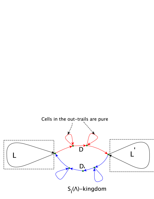
Figure 16. The re-decomposition of the Euler tour $Q$

Let $S_{i}(\Lambda)$ be a non-special bi-partition cell, then $S_{i}(\Lambda)$ is visited by two elements in $\{Q_{j};1\leq j\leq m\}$, say, $Q_{k}$ and $Q_{k^{\prime}}$. By Lemma 10.1, exactly two outpaths of $S_{i}(\Lambda)$, denoted by $L$ and $L^{\prime}$, contain special edges. Then the Euler tour $Q$ has the following decomposition:

$$Q=L+D+L^{\prime}+D^{\prime}.$$

We call $D\cup D^{\prime}$ the $S_{i}(\Lambda)$-kingdom, and call $D+D^{\prime}$ the partition of the $S_{i}(\Lambda)$-kingdom. Then $Q_{k}$, also $Q_{k}^{\prime}$, are cut into three parts by $L$ and $L^{\prime}$, and we denote the three parts by

(10.4) $$Q_{k}=C+D+E,\quad Q_{k^{\prime}}=C^{\prime}+D^{\prime}+E^{\prime},$$

where $C,E^{\prime}\subset L$ and $E,C^{\prime}\subset L^{\prime}$. (See Figure 17.) As a consequence of (10.4), we have

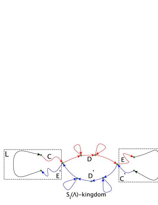
Figure 17. The decomposition of $Q_{k}$ and $Q_{k}^{\prime}$

Lemma 10.3.

An $S_{i}(\Lambda)$-kingdom is a cell-exact subgraph; moreover, all cells in it are pure except $S_{i}(\Lambda)$.

Lemma 10.4.

(Disjointness of Kingdoms.) Let $S_{i}(\Lambda)$ and $S_{j}(\Lambda)$ be two non-special bi-partition cells. Then the $S_{i}$-kingdom and the $S_{j}$-kingdom are disjoint.

Proof.

Since $S_{i}(\Lambda)$ is a bi-partition cell, $Q$ can be written as

$$Q=L+D+L^{\prime}+D^{\prime}$$

where $D+D^{\prime}$ is the $S_{i}$-kingdom. The cell $S_{j}(\Lambda)$ does not belong to the $S_{i}$-kingdom since it is not pure (see Lemma 10.3), so $S_{j}(\Lambda)$ must belong to one of $L$ and $L^{\prime}$. Let us assume that $S_{j}(\Lambda)\subset L^{\prime}$ without loss of generality. Then

$$Q\setminus L=L^{\prime}+(S_{i}\text{-kingdom})$$

is a closed subtrail of $Q$ not intersecting $S_{j}(\Lambda)$. So $Q\setminus L$ must belong to an outpath $L^{*}$ w.r.t. $S_{j}(\Lambda)$. This outpath $L^{*}$ contains $L^{\prime}$ and hence contains special edges, so it does not belong to the $S_{j}$-kingdom. It follows that the $S_{i}$-kingdom, as a subset of $L^{*}$, does not intersect the $S_{j}$-kingdom. The lemma is proved. ∎

10.3. Operation cells

First, let us reformulate the notion of primitivity. Let $Q$ be an Euler-partition. We construct a graph $T(Q)$ as following: the vertex set is $\{1,\dots,m\}$. If $Q_{k}$ contains a cell $S_{j}(\overrightarrow{a_{k^{\prime}}a_{k^{\prime}+1}})$ or $S_{j}(\overrightarrow{a_{k^{\prime}}a_{k^{\prime}+1}}^{-1})$ for some $j\in\Sigma$, then there is an edge from $k$ to $k^{\prime}$. Then $Q$ is primitive if and only if there is an integer $n_{0}$, for any $i,j\in\{1,\dots,m\}$, there is a trail in $T(Q)$ of length $n_{0}$ from $i$ to $j$.

Set

$$V=\{k~{};~{}~{}Q_{k}\text{ contains pure cells}\},\quad V^{\prime}=\{1,\dots,m\}/V.$$

If $V^{\prime}=\emptyset$, then $T(Q)$ is a complete graph and clearly $Q$ is primitive. So we assume that $V^{\prime}\neq\emptyset$. Let $k_{0}$ be the minimal element of $V^{\prime}$.

For each $k\in V$, we select a pure cell contained in $Q_{k}$, and call it the protected cell, or a black cell, of $Q_{k}$. It is possible that this black cell is contained in a $S_{j}$-kingdom. If this happens, then we call $S_{j}(\Lambda)$ an indirectly protected cell, or grey cell, associated with $Q_{k}$. (This means that $S_{j}(\Lambda)$ is a non-special bi-partition cell). By the disjointness of kingdoms, there is at most one grey cell associated with $Q_{k}$.

For any $k\in V^{\prime}$, $Q_{k}$ only visits bi-partition cells and poly-partition cells. We shall choose operation cells among the bi-partition cells which are visited by $Q_{k}$, non-special and are not grey cells; the lemma below estimates the number of such cells. Let $|Q_{j}|$ be the length of $Q_{j}$, i.e. the number of edges in $Q_{j}$.

Lemma 10.5.

Let $k\in V^{\prime}$. If

(10.5) $$\min_{1\leq j\leq m}|Q_{j}|\geq m^{4}+5m^{2},$$

then the number of bi-partition cells which are visited by $Q_{k}$, non-special and not indirectly protected, is at least $2m$.

Proof.

The total number of special cells, non-special poly-partition cells, and the indirectly protected cells are no more than $2m$, $\frac{m(m-1)(m-2)}{6}$ and $m$, respectively (see Lemma 10.2.). The number of cells visited by $Q_{k}$ is at least $|Q_{k}|/m$. So the number of the desired cells is no less than $|Q_{k}|/m-(2m+\frac{m(m-1)(m-2)}{6}+m)\geq 2m.$ ∎

Now we assume that the condition of Lemma 10.5 is fulfilled. Denote

$$r=m+(\#V^{\prime})-1.$$

By the above lemma, we can choose $r$ non-special, not indirectly protected, bi-partition cells

(10.6) $$T_{1},\dots,T_{m},T_{m+1},\dots,T_{r}$$

such that $Q_{k_{0}}$ (where $k_{0}=\min V^{\prime}$) visits the first $m$ of them, and for the other $k\in V^{\prime}$, each $Q_{k}$ visits a different cell in $T_{m+1},\dots,T_{r}$. We call them operation cells. In other words, we associate with $k_{0}$ the first $m$ operation cells, and for each $k\in V^{\prime}\setminus\{k_{0}\}$, we associate with one operation cell.

10.4. $(v,k)$-operation

Let $v$ be an edge of $\Lambda$ and let $k\in V^{\prime}$. Let $S_{\ell}(\Lambda)$ be an operation cell associated with $k\in V^{\prime}$. We do a $(v,k)$-operation to $S_{\ell}$ as follows.

Let $Q_{k^{*}}$ be the other trail in $\{Q_{j};~{}1\leq j\leq m\}$ visiting the cell $S_{\ell}(\Lambda)$. Let $D+D^{*}$ be the partition of the $S_{\ell}$-kingdom. By (10.4), $Q_{k}$ and $Q_{k^{*}}$ can be written as

$$Q_{k}=C+D+E,\quad Q_{k^{*}}=C^{*}+D^{*}+E^{*}$$

If $S_{\ell}(v)$ belongs to $Q_{k}$, the $v$-operation is a null operation, that is, we do not change $Q$. Otherwise, the $v$-operation is to construct a new Euler-partition $Q^{\prime}=Q_{1}^{\prime}+\cdots+Q_{m}^{\prime}$ by exchanging $D$ and $D^{*}$, precisely, we set

$$Q_{k}^{\prime}=C+(D^{*})^{-1}+E,\quad Q_{k*}^{\prime}=C^{*}+D^{-1}+E^{*},$$

and for $j\not\in\{k,k^{*}\}$, set $Q_{j}^{\prime}=Q_{j}$. Then the following statements (i)-(iv) hold:

$(i)$ $Q^{\prime}$ is an Euler tour in $G(S,A,\beta^{\prime})$ where $\beta^{\prime}$ is obtained by changing the orientation of all the cells in the $S_{\ell}$-kingdom. (This is clearly from the construction.)

$(ii)$ $Q^{\prime}$ contains pure cells if $Q$ does; (This is true, since if $Q_{j}$ contains a pure cell, the protected cell of $Q_{j}$ still belongs to $Q_{j}$ since the operation does not change any protected cell.)

$(iii)$ $Q^{\prime}$ is still consistent since $Q_{k}^{\prime}$ and $Q_{k}$ have the same initial and terminate points, $1\leq k\leq m$.

$(iv)$ Either $S_{\ell}(v)$ or $S_{\ell}(v^{-1})$ belongs to $Q_{k}^{\prime}$. (If $S_{\ell}(v)$ does not belong to $Q_{k}$, then it must appear in $D^{*}$. After operation, $S_{\ell}(v^{-1})$ belongs to $Q_{k}$.)

Now we can proof the main theorem of this section.

Proof of Theorem 10.1. Write $\Lambda=v_{1}+\cdots+v_{m}$. For $j=1,\dots,m$, we do $(v_{j},k_{0})$-operation to the $j$-th cell in (10.6), which are operation cells associated with the minimal element $k_{0}$ in $V^{\prime}$. For the operation cells associated to the indices $k\in V^{\prime}\setminus\{k_{0}\}$, we do the $(v_{k_{0}},k)$-operation. We can do these $r$ operations consecutively, since the operation cells belonging to the kingdoms are disjoint.

Let $Q^{\prime}=Q^{\prime}_{1}+\cdots Q^{\prime}_{m}$ be the resulted Euler-partition after doing all the operations.

First, $Q^{\prime}$ is an Euler-partition of $G({\mathcal{S}},A,\beta^{\prime})$, where $\beta^{\prime}$ is obtained by changing the orientations of the cells in the kingdoms which are involved in the operations.

Secondly, $Q^{\prime}$ is consistent, since all the operations do not change the origins and terminates of the partition.

Thirdly, $Q^{\prime}$ is primitive, since $v_{k_{0}}$ appears in every $Q_{k}$ for $k\in\{1,\dots,m\}$, and all $v_{j}$, $j=1,\dots,m$, appear in $Q_{k_{0}}$.

Finally, the pure cell property is clearly preserved. The theorem is proved. $\Box$

11. Proof of Theorem 1.4

In this section, we prove Theorem 1.4. We consider two cases according to the behaviour of the Hata graphs $H({\mathcal{S}}^{n},A)$, $n\geq 1$: if $H({\mathcal{S}}^{n},A)$ is not a chain for some $n\geq 1$, then we show that $K$ admits SFCs constructed by the Euler tour method; otherwise, ${\mathcal{S}}$ is a self-similar zipper.

A graph with $n$ vertices is a chain if there exists an order $x_{1},\dots,x_{n}$ of the vertices such that there is exactly one edge between $x_{i}$ and $x_{j}$ if $|i-j|=1$, otherwise there is no edge.

Theorem 11.1.

Let ${\mathcal{S}}=\{S_{i}\}_{i\in\Sigma}$ be an IFS satisfying the OSC. Suppose that ${\mathcal{S}}$ has skeleton $A$ and the Hata graph $H({\mathcal{S}}^{k},A)~{}(k\geq 1)$ is not always a chain. Then there exist an integer $n$, a permutation $\tau$ of $\{1,\dots,m\}$, a vector $\beta\in\{-1,1\}^{N^{n}}$ and an Euler-partition

$$P=P_{1}+\cdots+P_{m}$$

of $G({\mathcal{S}}^{n},A_{\tau},\beta)$ such that $P$ is consistent, primitive and potentially contains pure cells.

Proof.

By the assumption, there exists an integer $n_{1}$ such that the Hata graph $H({\mathcal{S}}^{n_{1}},A)$ is not a chain. By Theorem 9.1, there exist an integer $n_{2}$ and a permutation $\tau$ on $\{1,\dots,m\}$, and an Euler-partition

$$Q=Q_{1}+\cdots+Q_{m}$$

of $G({\mathcal{S}}^{n_{1}n_{2}},A_{\tau})$ such that $Q$ is consistent. Moreover, $Q$ contains more than $3$ unbroken cells by Remark 9.3.

Notice that $Q^{\ell}$, the $\ell$-th iteration of $Q$, is still consistent and contains more than $3$ unbroken cells. If we choose $\ell$ large enough, then the length of each $(Q^{\ell})_{j}$ can be large enough to satisfy inequality (10.1), so $Q^{\ell}$ satisfies all conditions of Theorem 10.1. Therefore, there exist an orientation vector $\beta$, and an Euler-partition $P=P_{1}+\cdots+P_{m}$ of $G({\mathcal{S}}^{n_{1}n_{2}\ell},A_{\tau},\beta)$ such that $P$ is consistent and primitive.

Finally, we show that $P$ contains pure cells. Since $2^{\ell}>2m$ when $\ell$ is large enough, by Lemma 9.2(iii), $Q^{\ell}$ contains more than $2m$ unbroken cells. Since there are only $2m$ special edges in the Euler-partition $Q^{\ell}$, there exists an unbroken cell which contains no special edge. This unbroken cell, as a subtrail of $Q^{\ell}$, can not cross the border of any elements in the partition $Q^{\ell}$, so it must be a pure cell of $Q^{\ell}$. Therefore, by Theorem 10.1, $P$ also contains pure cells. ∎

Recall that $\Sigma=\{1,2,\dots,N\}$.

Theorem 11.2.

Let ${\mathcal{S}}=\{S_{i}\}_{i\in\Sigma}$ be an IFS with connected invariant set $K$ satisfying the OSC. Suppose that $A$ is a skeleton of $K$ such that the Hata graph $H({\mathcal{S}}^{n},A)$ is a chain for every $n\geq 1$, then an arrangement of $\{S_{i}\}_{i\in\Sigma}$ is a self-similar zipper.

Proof.

We will abbreviate $H({\mathcal{S}}^{n},A)$ as $H_{n}$. Since $H_{1}$ is a chain, without lose of generality, we assume that $H_{1}$ passes the vertices in the order $S_{1},S_{2},\dots,S_{N}$. To simplify the notation, we denote $H_{1}$ by

$$H_{1}=(1,2,\dots,N)$$

instead of $(S_{1},S_{2},\dots,S_{N})$. Moreover, we set $1$ to be the origin of the chain and $N$ the terminus. For $1\leq j\leq N$, by self-similarity,

(11.1) $$({j1},{j2},\dots,{jN})\text{ or }({jN},\dots,{j2},{j1})$$

is a sub-chain of $H_{2}$, the starting vertex of $H({\mathcal{S}}^{2},A)$ is $S_{1k}$ for some $k\in\{1,N\}$, and the ending vertex is $S_{Nk^{\prime}}$ for some $k^{\prime}\in\{1,N\}$. Accordingly, we define a sequence $(\beta_{j})_{j=1}^{N}$ as following: $\beta_{j}=1$ if the former sequence in (11.1) is a sub-chain of $H({\mathcal{S}}^{2},A)$, and $\beta_{j}=-1$ otherwise.

We use $j(a_{1},\dots,a_{k})$ to denote the chain $(ja_{1},\dots,ja_{k})$, then we have

$$H_{2}=(1H_{1})^{\beta_{1}}+(2H_{1})^{\beta_{2}}+\dots+(NH_{1})^{\beta_{N}},$$

where we use $`+^{\prime}$ to denote the concatenation of two sequences, and denote $(a_{1},\dots,a_{k})^{-1}=(a_{k},\dots,a_{1})$ to be the reverse of a chain.

First, we prove by induction that

(11.2) $$H_{n}=(1H_{n-1})^{\beta_{1}}+\cdots+(NH_{n-1})^{\beta_{N}}.$$

By self-similarity, for any $j\in\{1,\dots,N\}$, either $jH_{n-1}$ or $(jH_{n-1})^{-1}$ is a sub-chain of $H_{n}$, so there exist $\epsilon_{1},\dots,\epsilon_{N}\in\{-1,1\}$ such that

$$H_{n}=(1H_{n-1})^{\epsilon_{1}}+\cdots+(NH_{n-1})^{\epsilon_{N}}.$$

Since $(jH_{n-1})^{-1}=j(H_{n-1})^{-1}$, using induction hypothesis, we have

$$\begin{array}[]{rl}H_{n}=&1(H_{n-1})^{\epsilon_{1}}+\cdots+N(H_{n-1})^{\epsilon_{N}}\\ =&\cdots+j\left(1H_{n-2}^{\beta_{1}}+\cdots+NH_{n-2}^{\beta_{N}}\right)^{\epsilon_{j}}+(j+1)\left(1H_{n-2}^{\beta_{1}}+\cdots+NH_{n-2}^{\beta_{N}}\right)^{\epsilon_{j+1}}+\cdots\end{array}$$

Notice that if $i_{1}\cdots i_{n}$ and $j_{1}\cdots j_{n}$ are adjacent in $H_{n}$, then $i_{1}\cdots i_{k}$ and $j_{1}\cdots j_{k}$ are adjacent in $H_{k}$ for any $k<n$. The above decomposition of $H_{n}$ forces that

$$j(1,\dots,N)^{\epsilon_{j}}+(j+1)(1,\dots,N)^{\epsilon_{j+1}}$$

is a sub-chain of $H_{2}$, so $\epsilon_{j}=\beta_{j}$ and $\epsilon_{j+1}=\beta_{j+1}$, which proves (11.2).

Using $(\beta_{1},\dots,\beta_{N})$, we define the following ordered GIFS:

(11.3) $$\begin{split}E_{1}=&S_{1}(E_{\beta_{1}})+S_{2}(E_{\beta_{2}})+\dots+S_{N}(E_{\beta_{N}})\\ E_{-1}=&S_{N}(E_{-\beta_{N}})+\dots+S_{2}(E_{-\beta_{2}})+S_{1}(E_{-\beta_{1}}).\end{split}$$

Clearly, $K=E_{1}=E_{-1}$ by the uniqueness of invariant set of ${\mathcal{S}}$.

Precisely, the vertex set of the GIFS is $\{E_{1},E_{-1}\}$. Let $\Gamma$ be the basic graph of the GIFS, then the $j$-th edge from $E_{1}$ is an edge from $E_{1}$ to $E_{\beta_{j}}$ with similitude $S_{j}$, which we denote by $(E_{1},S_{j},j,E_{\beta_{j}})$; the $j$-th edge starting from $E_{-1}$ goes to $E_{-\beta_{N-j+1}}$ and has similitude $S_{N-j+1}$, which we denote by $(E_{-1},S_{N-j+1},j,E_{-\beta_{N-j+1}})$.

By Theorem 1.3, to prove the theorem, we need only prove (11.3) is a linear GIFS.

Let $G_{n}$ be the sequence of trails in the graph $\Gamma$ emanating from the state $E_{1}$, arranged in the increasing order. Notice that for each trails in $G_{n}$, the associated contraction has the form $S_{I}$ with $|I|=n$, and for different trails, the associated contractions are distinct. So, we replace each trail in $G_{n}$ by the associated contraction and further more replace $S_{I}$ by the word $I$, then we obtain a sequence which is a permutation of $\Sigma^{n}$. For simplicity, we still denote this sequence by $G_{n}$. Similarly, we denote by $G_{n}^{\prime}$ the sequence of trails in the graph emanating from the state $E_{-1}$, arranged in the increasing order. We apply the same simplification to $G_{n}^{\prime}$.

We shall prove that $G_{n}=H_{n}$ and $G_{n}^{\prime}=G_{n}^{-1}$.

Clearly, $G_{1}=(1,2,\dots,N)$, $G_{1}^{\prime}=(N,\dots,1)$. Moreover, by (11.3),

$$G_{2}=(1G_{1})^{\beta_{1}}+\cdots+(NG_{1})^{\beta_{N}}.$$

We claim that, for every $n\geq 1$, it holds that

(11.4) $$G_{n}=(1G_{n-1})^{\beta_{1}}+\cdots+(NG_{n-1})^{\beta_{N}}$$

and $G_{n}^{\prime}=G_{n}^{-1}$.

We prove by induction on $n$. Let us consider the words in $G_{n}$ initialed by $j$. If $\beta_{j}=1$, then after one step, we are still in the state $E_{1}$, hence the arrangement of such words in increasing order is $jG_{n-1}$; if $\beta_{j}=-1$, we switch to the state $E_{-1}$ after one step, and the corresponding arrangement is $jG_{n-1}^{\prime}=j(G_{n-1})^{-1}$. Therefore,

$$G_{n}=(1G_{n-1})^{\beta_{1}}+(2G_{n-1})^{\beta_{2}}+\cdots+(NG_{n-1})^{\beta_{N}}.$$

The same argument shows that

$$\begin{array}[]{rl}G_{n}^{\prime}=&(NG_{n-1}^{\prime})^{\beta_{N}}+\cdots+(2G^{\prime}_{n-1})^{\beta_{2}}+(1G^{\prime}_{n-1})^{\beta_{1}}\\ =&(NG_{n-1})^{-\beta_{N}}+\cdots+(2G_{n-1})^{-\beta_{2}}+(1G_{n-1})^{-\beta_{1}}\\ =&G_{n}^{-1}.\end{array}$$

The claim is proved.

Comparing (11.2) and (11.4), we obtain that $G_{n}=H_{n}$ for all $n\geq 1$. Hence, if $I$ and $I^{\prime}$ are two adjacent words in $G_{n}$ (or in $G_{n}^{\prime}$), then they are also adjacent in $H_{n}$, so

$$S_{I}(K)\cap S_{I^{\prime}}(K)\supset S_{I}(A)\cap S_{I^{\prime}}(A)\neq\emptyset,$$

which implies that (11.3) is a linear GIFS.

∎

Proof of Theorem 1.4. Let $\{S_{i}\}_{i\in\Sigma}$ be an IFS satisfying the OSC. Let $A$ be a skeleton of ${\mathcal{S}}$.

If the Hata graph $H({\mathcal{S}}^{n},A)$ is alway a chain, then $K$ can be generated by a self-similar zipper by Theorem 11.2, and hence admits space-filling curves.

If $H({\mathcal{S}}^{n},A)$ is not alway a chain, by Theorem 11.1, there exists a integer $k$ such that an Euler-partition of $G({\mathcal{S}}^{k},A,\beta)$ satisfying the conditions in Theorem 8.2. Hence the invariant set of ${\mathcal{S}}^{k}$, which is also $K$, admits space-filling curves constructed by the Euler-tour method. $\Box$

References

- [1] S. Akiyama and B. Loridant: Boundary parametrization of planar self-affine tiles with collinear digit set, Sci. China Math., 53 (2010), 2173–2194.
- [2] J. Arndt: Plane-filling curves on all uniform grids, 2016, arXiv:1607.02433 [math.CO].
- [3] V. V. Aseev, A.V. Tetenov and A. S. Kravchenko: Self-similar Jordan curve on the plane, Sibirsk. Mat. Zh., 44 (2003), no. 3,481-492; English transl., Siberian Math. J., 44 (2003), no. 3, 379-386.
- [4] K. Astala: Self-similar zippers. Holomorphic functions ans moduli, Vol.I (berkeley, CA, 1986),Math. Sci. Res. Inst. Publ., 10 (1988), Springer, New York, 61-73.
- [5] M. Bader: Space-filling curves. An introduction with applications in scientific computing, Texts in Computational Science and Engineering, 9. Springer, Heidelberg (2013).
- [6] R. Balakrishnan and K. Ranganathan: A Textbook of Graph Theory, Universitext, Springer, New York (2000).
- [7] C. Bandt and M. Mesing: Self-affine fractals of finite type, Banach Center Publication, 84 (2009) 131–148.
- [8] N. L. Biggs, E. K. Lloyd and R. J. Wilson: Graph Theory 1736-1936, Clarendon Press, Oxford, 1976.
- [9] D. Ciesielska: On the 100 anniversary of the Sierpiński space-filling curve, Wiadomoci Matematyczne 48 (2012), no. 2, 69.
- [10] C. Davis and D. E. Knuth: Number representations and dragon curves I,II, Recreational Math. 3 (1970), 66–81 and 133–149.
- [11] F. M. Dekking: Recurrent sets, Adv. in Math., 44 (1982), no. 1, 78–104.
- [12] G. de Rham: Sur quelques courbes définies par des équations fonctionnelles, Rend. Sem. Mat. Torino, 16 (1957), 101–113.
- [13] P. Duvall, J. Keesling, and A. Vince: The Hausdorff dimension of the boundary of a self-similar tile, J. London Math. Soc. (2) 61 (2000), 748-760
- [14] K. J. Falconer: Fractal Geometry, Mathematical Foundations and Applications, Wiley, New York, 1990.
- [15] H. Fukuda, M. Shimizu and G. Nakamura: New Gosper Space Filling Curves, Proceedings of the International Conference on Computer Graphics and Imaging (CGIM2001),(2001) 34-38 .
- [16] M. Gardner: In which “monster” curves force redefinitions of the word “curve”, Scientific American, 235 (1976), 124–133.
- [17] M. Hata: On the structure of self-similar sets, Japan J. Appl. Math., 2 (1985), 381–414.
- [18] D. Hilbert: Über die stetige abbidung einer Linie auf ein Flächenstuck, Math. Ann., 38 (1891), 459–460.
- [19] J. E. Hutchinson: Fractal and self similarity, Indian Univ. Math. J., 30 (1981), 713–747.
- [20] R. Kenyon: Self-replicating tilings. Symbolic dynamics and its applications (New Haven, CT, 1991), American Mathematical Society, Providence, RI, vol., 135 (1992), 239–263.
- [21] J. Kigami: Analysis on fractal Sets, Cambridge University Press, 2003.
- [22] J. C. Lagarias and Y. Wang: Self-affine tiles in ,Advan. Math. 121(1996), 21-49.
- [23] W. X. Li: Separation properties for MW-fractals, Acta Math. Sinica (Chin. Ser.), 41 (1998), no. 4, 721–726.
- [24] A. Lindenmayer: Mathematical models for cellular interacton in development, Parts I and II. Journal of Theoretical Bilology, 30 (1968), 280–315.
- [25] S. M. Ngai and Y. Wang: Hausdorff dimension of overlapping self-similar sets, J. London Math. Soc., 63 (2001), no. 2, 655–672.
- [26] D. Mauldin and S. Williams: Hausdorff dimension in graph directed constructions, Trans. Amer. Math. Soc., 309 (1988), 811–829.
- [27] S. C. Milne: Peano curves and smoothness of functions, Advances in Mathematics, 35 (1980), 129–157.
- [28] M. Morán: Dynamical boundary of a self-similar sets, Fund. Math., 160 (1999), no. 1, 1–14.
- [29] M. Newman: integral matrics, Academic Press, New York, 1972.
- [30] G. Peano: Sur une courbe qui remplit toute une qire plane, Math. Ann., 36 (1890), 157–160.
- [31] G. Pólya: Über eine Peanosche kurve, Bull. Acad. Sci. Cracovie (Sci. math. etnat. Série A), (1913), 1–9.
- [32] O. Purevdorj and A.V. Tetenov: The example of a self-similar continuum which is not an attractor of any zipper, arXiv:0812. 2462v1, [math.GT].
- [33] M. Queffélec: Substitution dynamical systems-spectral analysis, Lecture Notes in Mathematics 1294, Springer, Berlin, (1987).
- [34] H. Rao and Z. Y. Wen: A class of self-similar fractals with overlap structure, Adv. in Appl. Math. 20 (1998), 50-72.
- [35] H. Rao and S. Q. Zhang: Space-filling curves of self-similar sets (I): Iterated function systems with order structures, Nonlinearity,29 (2016), no.7, 2112-2132.
- [36] H. Rao and S. Q. Zhang: Space-filling curves of self-similar sets (III): Skeletons. In preparation.
- [37] M. Remes: Hölder parametrizations of self-similar sets, Ann. Acad. Sci. Fenn. Math. Diss., no. 112, (1998), 68 pp.
- [38] H. Sagan: Space-Filling Curve, Springer-Verlag, New York (1994).
- [39] A. Schief: Separation properties for self-similar sets, Proc. Amer. Math. Soc., 122 (1994), 114–115.
- [40] W. Sierpiński: Sur une nouvelle courbe continue qui remplit toute une aire plane, Bull. Acad. Sci. de Cracovie, (1912), 52-66.
- [41] V. F. Sirvent: Hilbert’s space filling curves and geodesic laminations, Math. Phys. Electron. J., 9 (2003), Paper 4, 13 pp. (electronic).
- [42] V. F. Sirvent: Space filling curves and geodesic laminations, Geometriae Dedicata., 135 (2008), 1–14.
- [43] V. F. Sirvent: Space-filling curves and geodesic laminations. II: Symmetries, Monatsh. Math. 166 (2012), no. 3–4, 543–558.
- [44] G. Teachout: Spacefilling curve designs featured in the web site: http://teachout1.net/village/.
- [45] A. Tetenov, K. Kamalutdinov and D. Vaulin: Self-similar Jordan arcs which do not satisfy OSC, arXiv:1512.00290v2 [math. MG].
- [46] W. P. Thurston, Zippers and univalent functions, Amer. Math. Soc., Providence, RI, 21 (1986), 185-197.
- [47] J. Ventrella: Fractal Curves in the web site :http://www.fractalcurves.com/.