Crossing probability for directed polymers in random media: exact tail of the distribution

Abstract

We study the probability $p\equiv p_{\eta}(t)$ that two directed polymers in a given random potential $\eta$ and with fixed and nearby endpoints, do not cross until time $t$. This probability is itself a random variable (over samples $\eta$) which, as we show, acquires a very broad probability distribution at large time. In particular the moments of $p$ are found to be dominated by atypical samples where $p$ is of order unity. Building on a formula established by us in a previous work using nested Bethe Ansatz and Macdonald process methods, we obtain analytically the leading large time behavior of all moments $\overline{p^{m}}\simeq\gamma_{m}/t$. From this, we extract the exact tail $\sim\rho(p)/t$ of the probability distribution of the non-crossing probability at large time. The exact formula is compared to numerical simulations, with excellent agreement.

I Introduction

I.1 Overview

The problem of directed paths, also called directed polymers, in a random potential arises in a variety of fieldsHuse et al. (1985); *kardar1987scaling; *halpin1995kinetic; Blatter et al. (1994); Lemerle et al. (1998); SoOr07 ; bec ; Gueudré et al. (2014); Hwa and Lässig (1996); Otwinowski and Krug (2014). In its continuum version, it is connected to the Kardar-Parisi-Zhang (KPZ) growth equation Kardar et al. (1986) by an exact mapping, the Cole-Hopf transformation. Recent progress in integrability of the KPZ equation in one dimension spohnKPZEdge ; Calabrese et al. (2010); dotsenko ; corwinDP ; Borodin and Corwin (2014); flat ; SasamotoStationary ; Quastelflat ; calabreseSine have thus been accompanied by new exact results for the directed polymer (DP) in $1+1$ dimension. Methods from physics such as replica and the Bethe Ansatz Kardar (1987); Calabrese et al. (2010); dotsenko ; flat ; SasamotoStationary , or from mathematics such as the Macdonald processes Borodin and Corwin (2014), led to many exact results both for the KPZ and the DP problem. Examples in the later case are distributions of the free energy, of the endpoint position Endpoint , as well as some multi-point correlations 2point .

Despite these progresses, many interesting DP observables still evade exact calculations. This is the case for instance of quantities testing the spatial structure of the manifold of DP ground states such as the statistics of coalescence times Pimentel , or of their low lying excited states, such as the overlap and the droplet probabilities, of great interest for many applications, e.g. to quantum localization markus_magneto . Similarly, very few results are available for the problem of several interacting DP which are mutually competing within the same random potential, most notably the case of several DP subjected to the constraint of non-crossing natter ; Emig and Kardar (2001); Ferrari (2004); Borodin and Corwin (2014); Doumerc . More generally, not much is known about crossing or non-crossing probabilities for paths in random media. Since in a random potential directed polymers compete for the same optimal configuration(s), one can expect that the non-crossing probability may be small. It remains to quantify how small they are and how rare are the samples such that they are not small.

In a recent work we introduced a general framework to calculate non-crossing probabilities for directed polymers, equivalently free energies of a collection of directed paths with a non-crossing constraint. Specifically, we studied the probability $p_{\eta}(t)$ that two directed polymers in the same white noise random potential $\eta\equiv\sqrt{2\bar{c}}~{}\eta(x,t)$ and with all four endpoints fixed nearby $x=0$ (see below precise definition) do not intersect up to time $t$. We used the replica method to map the problem onto the Lieb-Liniger model with attractive interaction $c=-\bar{c}<0$ and generalized statistics between particles. Employing both the Nested Bethe Ansatz and known formula from Macdonald processes, we obtained a general formula for the integer moments $\overline{p_{\eta}(t)^{m}}$ (overbar denotes averages with respect to $\eta$) which we could relate, at least at a formal level, to a Fredholm determinant. While explicit evaluation of this formula for any $m,t$ appeared very difficult, we were able to obtain explicit results for $m=1,2$ for all time $t$, and for $m=3$ in the large time limit. This led us to conjecture that, at large time:

$$\overline{p_{\eta}(t)^{m}}\simeq_{t\to\infty}\gamma_{m}\frac{\bar{c}^{2(m-1)}}{t}$$ (1)

where $\bar{c}$ is the strength of the disorder, with explicit values for the first three coefficients

$$\gamma_{1}=\frac{1}{2}\;,\quad\gamma_{2}=\frac{1}{12}\;,\quad\gamma_{3}=\frac{1}{15}\;.$$ (2)

The calculation of all the $\gamma_{m}$ and the more general question of the determination of the full probability distribution, ${\cal P}_{t}(p)$ of $p\equiv p_{\eta}(t)$, remained open problems. An interesting finding of De Luca and Le Doussal (2015) is that the first moment is exactly given by (1) i.e. $\overline{p_{\eta}(t)}=1/(2t)$ for all $t$, independent of the disorder strength, and in fact identical to the result without disorder. As explained there (and recalled below) this arises as a consequence of an exact symmetry of the problem, called the statistical tilt symmetry (STS).

I.2 Aim and main results

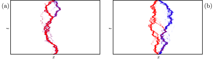
Figure 1: Configuration of two polymers starting at $(\hat{x}=\mp 1/2,\hat{t}=0)$ (respectively red/blue) for a typical value of $p$ in (a) and for a rare realization with large $p=O(1)$ in (b). The opacity of each dot in $(\hat{x},\hat{t})$ corresponds to $Z(\pm 1/2,\hat{x}|\hat{t})\times Z(\hat{x},\pm 1/2|\hat{\tau}-\hat{t})$ with $\hat{\tau}=300$. See Section IV.3 for definitions of notations on the lattice. Here, $\beta=1.0$ and the red points have been drawn on top of the blues, which explains the apparent asymmetry in (a).

The aim of this paper is to report a first step in the determination of the sample to sample distribution of non-crossing probability ${\cal P}_{t}(p)$. We will start from the general formula for the moments derived in De Luca and Le Doussal (2015) in terms of multiple integrals over so-called string rapidities, $\mu_{j}$, of a quite complicated symmetric polynomial of these rapidities (called $\Lambda_{n,m}(\mu)$ below). We will develop general algebraic methods to deal with these types of polynomials and integrals, and apply them here to study the replica limit $n=0$ and the large time limit. We demonstrate that the conjecture (1) is indeed correct and obtain all the coefficients $\gamma_{m}$. From the moments (1) we are able reconstruct an interesting and non-trivial information about the probability distribution ${\cal P}_{t}(p)$, namely its tail, as we now explain.

It is important to point out that the result (1) is valid only for fixed integer $m$ in the limit of large time. In fact, this knowledge of the leading behavior of the integer moments at large time is not sufficient to reconstruct the full distribution of $p$. As we have argued in supplmat_deluca2015 on the basis of universality from the results of Doumerc , we expect that

$$\ln p_{typ}(t)\equiv\overline{\ln p_{\eta}(t)}\sim-a(\bar{c}^{2}t)^{1/3}$$ (3)

where, furthermore, $a=\overline{\chi_{2}}-\overline{\chi^{\prime}_{2}}\approx 1.9043$ is the average gap between the first ($\chi_{2}$) and second ($\chi^{\prime}_{2}$) GUE largest (properly scaled) eigenvalues of a random matrix belonging to the Gaussian unitary ensemble (GUE). This means that in a typical realization of the random potential $\eta$, $p\equiv p_{\eta}(t)$ is sub-exponentially small at large time, i.e. $p_{typ}(t)\sim e^{-a(\bar{c}^{2}t)^{1/3}}$. To account for the form (1) the integer moments should be dominated by a small fraction $\sim 1/(\bar{c}^{2}t)$ of environments for which typically $p_{\eta}(t)\sim\bar{c}^{2}$. Hence we are led to conclude that

$${\cal P}_{t}(p)\simeq_{t\to+\infty}{\cal P}^{0}\bigl{(}p/p_{typ}(t)\bigr{)}+\frac{\rho(p/\bar{c}^{2})}{\bar{c}^{4}t}$$ (4)

where $\rho(p/\bar{c})$ is a fixed function and ${\cal P}^{0}$ is the bulk of the distribution centered around the typical value. Here our goal is to calculate only the tail function $\rho(p)$, leaving the determination of the bulk function to future studies. We obtain, from an exact calculation of the $\gamma_{m}$ (given in formula (58) below),

$$\rho(p)=\frac{2}{p}\int_{0}^{+\infty}\frac{du}{\sqrt{u(u+4)}}K_{0}(2\sqrt{p}\sqrt{u+4})$$ (5)

where $K_{0}$ is the modified Bessel function. It is easy to see that this result reproduces $\int dpp^{m}\rho(p)=\gamma_{m}$ in agreement with the values in Eq. (2). The conjecture (4) with the analytical form (5) is fully confirmed by our numerical study, see Sec. IV.3; in particular Fig. 2 shows comparison with the model defined on the square lattice, which at high temperature is a good approximation of the continuum one.

Strictly Eq. (4) and (5) are valid only at fixed $p$ for large $t$, and the total weight in the tail is naively $\sim 1/t$. However one sees that the asymptotic behavior of the density function $\rho(p)$ at small $p$ is

$$\rho(p)\simeq\frac{1}{2p}(\ln p)^{2}$$ (6)

hence its total weight is not integrable at small $p$. Thus we can surmise that the above form holds for $p>p_{c}(t)$ where $p_{c}(t)$ is a small-$p$ time-dependent cutoff, and we can try to match the tail to the bulk around $p_{c}(t)$. Integration of (6) gives a total weight $\sim\frac{1}{6}|\ln p_{c}(t)|^{3}/t$ for the tail region of the probability distribution. This suggests, assuming no other intermediate scale, the following bound on $p_{c}(t)$: $\frac{1}{6}|\ln p_{c}(t)|^{3}/t\ll 1$ i.e. $\ln p_{c}(t)\gg-(6t)^{1/3}\simeq-1.817t^{1/3}$. This is consistent with $p_{typ}(t)\ll p_{c}(t)$ but on the same $t^{1/3}$ scale. A more detailed analysis of this matching is left for the future.

Finally one may wonder how the samples with values of $p$ of order one differ in real space from the ones with typical values of $p$. For this, we show in Fig 1 density plots of the configurational probabilities of two independent directed polymers in the same environment constrained to start and end at different, but very close-by points (nearest neighbors on the lattice). We show two samples: for the sample with higher $p$, the small difference in starting points results in a very large difference in most probable configurations. The details of the numerics are discussed in section Sec. IV.3.

The paper is organized as follows: in Sec. II, we recall the model, the observables and the main results of De Luca and Le Doussal (2015) which are the starting point for the present calculation; in Sec. III, we study the building blocks for the formula of the moments of $p_{\eta}(t)$; finally in Sec. IV, we apply these formulas in the limit $n\to 0$ and of large times to derive the coefficients $\gamma_{m}$ and the distribution of $p_{\eta}(t)$, which is then compared to numerics.

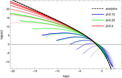
Figure 2: Comparison of our prediction for the continuum model with numerical simulations of the DP on the square lattice, as described in the text. We use at least $2\times 10^{5}$ realizations of the disorder (samples). The $\log$ of the empirical distributions of $p=\hat{p}/(16\beta^{4})$, with $\hat{p}$ the probability on the lattice, is shown for different values of $\beta$ and several times $\hat{t}=2^{8},2^{9},\ldots,2^{13}$. The opacity of each line is scaled proportionally $\hat{t}$. The analytical prediction in Eq. (60) for the tail of the distribution is confirmed at large times $\hat{t}\to\infty$ and $\beta\to 0$. Note that the bulk of the distribution and $\ln p_{typ}(t)$ shifts very rapidly to large negative values (which we find consistent with $t^{1/3}$, but not analyzed here).

II Model, observables and starting formula

II.1 Model and observables

The model of a directed polymer in the continuum in dimension $1+1$ is defined by the partition sum of all paths $x(\tau)\in\mathbb{R}$ starting from $x$ at time $\tau=0$, and ending at $y$ at time $\tau=t$. This can be seen as the canonical partition function of a directed polymer of length $t$ with fixed endpoints

$$Z_{\eta}(x;y|t)\equiv\int_{x(0)=x}^{x(t)=y}Dxe^{-\int_{0}^{t}d\tau\left[\frac{1}{4}(\frac{dx}{d\tau})^{2}-\sqrt{2\bar{c}}\eta(x(\tau),\tau)\right]}$$ (7)

in a random potential with white-noise correlations $\overline{\eta(x,t)\eta(x^{\prime},t^{\prime})}=\delta(x-x^{\prime})\delta(t-t^{\prime})$. It describes the thermal fluctuations of a single polymer in a given realization $\eta$ of the random potential (a sample).

Thanks to the Karlin-McGregor formula for non-crossing paths and its generalizations Karlin et al. (1959); *gessel1985binomial; *gessel1989determinants; *wiki:lgvlem, the partition sum of two polymers with ordered and fixed endpoints, $(x_{1},y_{1})$ and $(x_{2},y_{2})$, is given by a determinant formed with the single polymer partition sums:

$$Z^{(2)}_{\eta}(x_{1},x_{2};y_{1},y_{2}|t)=Z_{\eta}(x_{1};y_{1}|t)Z_{\eta}(x_{2};y_{2}|t)-Z_{\eta}(x_{2};y_{1}|t)Z_{\eta}(x_{1};y_{2}|t)\;.$$ (8)

Hence one can express the probability (over thermal fluctuations) that two polymers with fixed endpoints do not cross in a given realization $\eta$ as the ratio:

$$p_{\eta}(x_{1},x_{2};y_{1},y_{2}|t)\equiv 1-\frac{Z_{\eta}(x_{2};y_{1}|t)Z_{\eta}(x_{1};y_{2}|t)}{Z_{\eta}(x_{1};y_{1}|t)Z_{\eta}(x_{2};y_{2}|t)}\;.$$ (9)

Here for simplicity, we study only the random variable defined by the limit of near-coinciding endpoints

$$p_{\eta}(t)\equiv\lim_{\epsilon\to 0}\frac{p_{\eta}(-\epsilon,\epsilon;-\epsilon,\epsilon|t)}{4\epsilon^{2}}$$ (10)

As noticed in De Luca and Le Doussal (2015), it can also be written as:

$$p_{\eta}(t)=\left.\partial_{x}\partial_{y}\ln Z_{\eta}(x;y|t)\right|_{\begin{subarray}{c}x=0\\ y=0\end{subarray}}$$ (11)

which is useful in some cases, e.g. to show that the first moment is independent of the disorder, see De Luca and Le Doussal (2015).

II.2 Replica trick and starting formula

The observables that we will study here are the integer moments of this probability $p_{\eta}(t)$. Using the replica trick these moments can be written as

$$\overline{p_{\eta}(t)^{m}}=\lim_{n\to 0}\Theta_{n,m}(t)$$ (12)

where we have introduced:

$$\Theta_{n,m}(t)\equiv\lim_{\epsilon\to 0}\overline{[(2\epsilon)^{-2}Z_{\eta}^{(2)}(\epsilon)]^{m}[Z_{\eta}(0;0|t)]^{n-2m}}$$ (13)

and we defined the partition sum of two non-crossing polymers with endpoints near $x=0$ as

$$Z^{(2)}_{\eta}(\epsilon)\equiv Z_{\eta}(\epsilon;\epsilon|t)Z_{\eta}(-\epsilon;-\epsilon|t)-Z_{\eta}(-\epsilon;\epsilon|t)Z_{\eta}(\epsilon;-\epsilon|t)$$ (14)

The idea is now to calculate $\Theta_{n,m}(t)$ and then to take the limit $n=0$.

In Ref. De Luca and Le Doussal (2015), we have derived a formula for these quantities. This result was obtained in the simplest case ($m=1$) by use of the nested Bethe Ansatz and, for general $m$, using a contour integral formula obtained from the theory of Macdonald processes in Borodin and Corwin (2014), with perfect agreement between the two methods.

The formula goes as follows. For each $n,m$, one first defines a function of a set of $n$ complex variables $\mu_{\alpha}$, $\alpha=1,..n$, the “rapidities” (also indicated collectively by a vector $\bm{\mu}=(\mu_{1},\ldots,\mu_{n})$) as

$$\Lambda_{n,m}(\bm{\mu})=\frac{1}{2^{m}}\operatorname{sym}_{\bm{\mu}}\left[\frac{\prod_{q=1}^{m}h(\mu_{2q-1,2q})}{\prod_{1\leq\alpha<\beta\leq n}f(\mu_{\beta\alpha})}\right]$$ (15)

where $\mu_{\beta\alpha}=\mu_{\beta}-\mu_{\alpha}$ and we have introduced the two functions

$$h(u)=u(u-ic)\quad,\quad f(u)=u/(u-ic)$$ (16)

and the symmetrization operator over the variables $\mu$:

$$\operatorname{sym}_{\bm{\mu}}[F(\mu_{1},\ldots,\mu_{n})]=\frac{1}{n!}\sum_{P\in\mathcal{S}_{n}}F(\mu_{P_{1}},\ldots,\mu_{P_{n}})\;.$$ (17)

As discussed below, the rational function in Eq. (15) is actually a symmetric polynomial in the $\mu_{\alpha}$.

The formula obtained in De Luca and Le Doussal (2015) then reads:

$$\Theta_{n,m}(t)=\langle\Lambda_{n,m}(\bm{\mu})\rangle_{n}$$ (18)

where we introduced the “string average” for any symmetric function $F(\bm{\mu})$ as

$$\langle F(\bm{\mu})\rangle_{n}\equiv\sum_{n_{s}=1}^{n}\frac{n!\bar{c}^{n}}{n_{s}!(2\pi\bar{c})^{n_{s}}}\sum_{(m_{1},..m_{n_{s}})_{n}}\prod_{j=1}^{n_{s}}\int_{-\infty}^{+\infty}\frac{dk_{j}}{m_{j}}\Phi(\mathbf{k},\mathbf{m})F^{s}(\mathbf{k},\mathbf{m})e^{-\mathcal{A}_{2}^{s}(\mathbf{k},\mathbf{m})t}\;.$$ (19)

In this equation, we introduce the notation

$$F^{s}(\mathbf{k},\mathbf{m})\equiv F(\bm{\mu})|_{{\bf\mu}={\bf\mu^{s}}}\;,\qquad\Phi(\mathbf{k},\mathbf{m})=\prod_{1\leq j<j^{\prime}\leq n_{s}}\frac{(k_{j}-k_{j^{\prime}})^{2}+\bar{c}^{2}(m_{j}-m_{j^{\prime}})^{2}/4}{(k_{j}-k_{j^{\prime}})^{2}+\bar{c}^{2}(m_{j}+m_{j^{\prime}})^{2}/4}\;,$$ (20)

$$\mu^{s}_{\alpha}\equiv\mu^{s}_{j,a}=k_{j}+\frac{i\bar{c}}{2}(m_{j}+1-2a)\;,\quad a_{j}=1,..m_{j}\;,\quad j=1,..n_{s}\;,$$ (21)

$$\mathcal{A}_{p}(\bm{\mu})\equiv\sum_{\alpha=1}^{n}\mu_{\alpha}^{p}\;,\quad{\cal A}_{p}^{s}(\mathbf{k},\mathbf{m})\equiv\mathcal{A}_{p}(\bm{\mu})|_{{\bf\mu}={\bf\mu^{s}}}$$ (22)

where $A_{2}$ denotes the energy and $\mathcal{A}_{p}$ corresponds to the conserved charges of the Lieb-Liniger model ll . The factor $F^{s}(\mathbf{k},\mathbf{m})$ is obtained from $F(\bm{\mu})$ replacing the values of the $n$ rapidities $\mu_{\alpha}$ with their values $\mu^{s}_{j,a}$ for a “string state” and so is $\mathcal{A}_{p}^{s}(\mathbf{k},\mathbf{m})$ obtained from $\mathcal{A}_{p}(\bm{\mu})$. Such a “string state” is characterized by: (i) an integer $n_{s}$, the number of strings in the state, with $1\leq n_{s}\leq n$; (ii) $n_{s}$ real variables $k_{j}\in\mathbb{R}$, $j=1,\ldots,n_{s}$, the “momenta of the string center of mass”; (iii) $n_{s}$ integer variables $1\leq m_{j}$, ”the particle content” of each string in the string state. In the above formula (19) a “summation” over all string states is performed, meaning that these variables are summed upon or integrated upon. Here, $(m_{1},\ldots,m_{n_{s}})_{n}$ indicates sum over all integers $m_{j}\geq 1$ whose sum equals $n$, i.e. $\sum_{j=1}^{n_{s}}m_{j}=n$.

An important property of (18) and (19) is that considering $\langle\Lambda_{n,0}\rangle_{n}\equiv\langle 1\rangle_{n}$, one recovers the formula for $\mathcal{Z}_{n}(t)\equiv\mathcal{Z}_{n}(\mathbf{x}=\bm{0};\bm{0}|t)=\Theta_{n,0}(t)$ for the $n$-th moment of a single DP partition sum with fixed endpoint, studied and calculated in Calabrese et al. (2010). The present calculation is thus a, quite non-trivial, generalization of that calculation.

The formula (18) is thus our starting point. We now turn to explicit calculations of the building blocks in Eq. (15).

III Calculation of the building blocks $\Lambda_{n,m}({\bf\mu})$

In this section we provide an explicit formula for $\Lambda_{n,m}(\bm{\mu})$ as a symmetric polynomial. This approach is based on: (i) the invariance of (15) under the simultaneous translation of all the rapidities $\mu_{\alpha}\to\mu_{\alpha}+u$; (ii) the fact that $\Lambda_{n,m}$ vanishes on any $\ell$-string with $\ell>n-m$.

The best way to deal with this problem, is to separate these polynomials into homogeneous components, which are discovered to coincide with the $\Lambda_{n,m}(\bm{\mu})$ computed at $\bar{c}=0$. Hence, we start by studying this case.

III.1 $\bar{c}=0$ case

We define $\tilde{\Lambda}_{n,m}(\bm{\mu})$ as $\Lambda_{n,m}(\bm{\mu})$ computed at $\bar{c}=0$. In this case $f(u)=1$ in (16) and therefore Eq. (15) simplifies to

$$\tilde{\Lambda}_{n,m}(\bm{\mu})=\frac{1}{2^{m}}\operatorname{sym}_{\bm{\mu}}\left[\prod_{q=1}^{m}(\mu_{2q-1}-\mu_{2q})^{2}\right]=\operatorname{sym}_{\bm{\mu}}\left[\prod_{q=1}^{m}(\mu_{2q-1}^{2}-\mu_{2q-1}\mu_{2q})\right]$$ (23)

where the second equality is obtained expanding the square and replacing $\mu_{2q}\to\mu_{2q-1}$ inside the symmetrization. We want to re-express (23) in terms of the elementary symmetric polynomials

$$e_{p}(\bm{\mu})=\sum_{1\leq\alpha_{1}<\ldots<\alpha_{p}\leq n}\mu_{\alpha_{1}}\ldots\mu_{\alpha_{p}}\;.$$ (24)

with $e_{0}(\bm{\mu})=1$ and we will use below the convention that $\mu_{\alpha}=0$ for $\alpha>n$, leading to $e_{p}(\bm{\mu})=0$ for $p>n$ . We will also omit the explicit dependence on rapidities when these do not take a specific value and simply denote $e_{p}\equiv e_{p}(\bm{\mu})$. It is important to underline few properties that (23) has to satisfy. Indeed, $\tilde{\Lambda}_{n,m}(\bm{\mu})$ is a polynomial

1. symmetric in the variables $\mu_{1},\ldots,\mu_{n}$;

2. homogeneous of degree $2m$;

3. containing each rapidity $\mu_{\alpha}$ with degree at most $2$;

4. invariant under a simultaneous translation of all variables: $\tilde{\Lambda}_{n,m}(\bm{\mu}+u)=\tilde{\Lambda}_{n,m}(\bm{\mu})$ for any complex number $u$ and $\bm{\mu}+u=(\mu_{1}+u,\ldots,\mu_{n}+u)$.

Conditions 1, 2, 3 impose that $\tilde{\Lambda}_{n,m}(\bm{\mu})$ is a linear combinations of terms $e_{p}e_{2m-p}$ with $p=0,\ldots,m$. Moreover, in this expansion, all the coefficients, but one, can be fixed using condition 4. An important consequence, which we will use below, is that, for any given $n,m$, a polynomial satisfying conditions 1–4 has to be a multiple of $\tilde{\Lambda}_{n,m}$. Additionally, by focusing on the coefficient of $\prod_{q}\mu_{2q-1}^{2}$ in (23), it can be seen that $e_{m}e_{m}$ appears multiplied by $m!(n-m)!/n!$. We refer to Appendix A for all the details and we get

$$\tilde{\Lambda}_{n,m}(\bm{\mu})=\frac{m!}{n!(n-m)!}(-1)^{m}\sum_{p=0}^{2m}(-1)^{p}(n-p)!(n-2m+p)!e_{p}e_{2m-p}$$ (25)

which is the required expansion. Remarkably, this expression is a convolution and can therefore be expressed compactly using generating functions. We recall the standard generating function for the elementary symmetric polynomials

$$E(x|\bm{\mu})=\prod_{i\geq 1}(1+\mu_{i}x)=\sum_{r\geq 0}e_{r}x^{r}\;.$$ (26)

Again we will write simply $E(x|\bm{\mu})\equiv E(x)$, and similarly for other generating functions, whenever the rapidities are considered at generic values. Then, we can rewrite

$$\tilde{\Lambda}_{n,m}(\bm{\mu})=\frac{m!}{n!(n-m)!}(-1)^{m}[H_{n}(x)H_{n}(-x)]_{x^{2m}}$$ (27)

where we introduced

$$H_{n}(x)=\sum_{p=0}^{n}(n-p)!e_{p}x^{p}=\int_{0}^{\infty}dte^{-t}t^{n}E(x/t)$$ (28)

and everywhere here $[F(x)]_{x^{p}}$ indicates the coefficient of $x^{p}$ in the series $F(x)$.

III.2 General case $\bar{c}\neq 0$

The study of the finite $\bar{c}$ case requires a more detailed analysis. First of all, one can check (see Appendix B.1) that $\Lambda_{n,m}(\bm{\mu})$ is still a symmetric polynomial in the rapidities. Moreover it is homogeneous of degree $2m$ in the combined set of $\bar{c},\mu_{1},\ldots,\mu_{n}$. Thanks to the characterization of $\tilde{\Lambda}_{n,m^{\prime}}(\bm{\mu})$ in terms of properties 1–4 given in the previous section, it can be seen (Appendix B.2) that $\Lambda_{n,m}(\bm{\mu})$ admits the following expansion

$$\Lambda_{n,m}(\bm{\mu})=\sum_{a=0}^{m}\bar{c}^{2a}\Omega_{n,m}^{a}\tilde{\Lambda}_{n,m-a}(\bm{\mu})\;,$$ (29)

where the $\Omega_{n,m}^{a}$ are constant coefficients, for the moment unknown, expect for $\Omega_{n,m}^{0}=1$. Thanks to Eq. (27), it is possible to rewrite Eq. (29) again in terms of generating functions as

$$\Lambda_{n,m}(\bm{\mu})=\frac{m!(-1)^{m}}{(n-m)!n!}[\omega_{n,m}(i\bar{c}x)H_{n}(x)H_{n}(-x)]_{x^{2m}}$$ (30)

where we introduced the generating function of the unknowns $\Omega_{n,m}^{a}$

$$\omega_{n,m}(x)=\frac{(n-m)!}{m!}\sum_{a=0}^{m}\Omega_{n,m}^{a}\frac{(m-a)!}{(n-m+a)!}x^{2a}$$ (31)

with $\omega_{n,m}(0)=1$. Since Eq. (29) and Eq. (30) holds for an arbitrary choice of $\bm{\mu}$, the values of the $\Omega_{n,m}^{a}$ can be fixed by choosing specific configuration of rapidities where $\Lambda_{n,m}(\bm{\mu})$ simplifies. Consider in particular the string configuration (21) characterized by $m_{1}=\ell$ and $m_{2}=\ldots=m_{n-\ell+1}=1$, all with vanishing momenta $k_{j}=0$, i.e.

$$\bm{\mu}^{\ell,0}=\left(\frac{i\bar{c}}{2}(\ell-1),\frac{i\bar{c}}{2}(\ell-3),\ldots,-\frac{i\bar{c}}{2}(\ell-1),0,\ldots,0\right)\;,$$ (32)

then one obtains (see Appendix B.3) that

$$\Lambda_{n,m}(\bm{\mu}^{\ell,0})=0\;,\qquad\mbox{for any}\;\ell=n-m+1,n-m+2,\ldots,n\;.$$ (33)

These conditions have a direct physical interpretation: in the Lieb-Liniger language, an $\ell$-strings can be considered as a bound-state composed by $\ell$ particles; in order to form a string with $\ell>n-m$, necessarily, the rapidities of two-particles which are mutually avoiding each other would need to be included in the string. As no bound state can be formed between avoiding particles, this term gives a vanishing contribution in Eq. (18). So, the condition expressed by (33) encodes the effective repulsion between polymers. The value of the elementary symmetric polynomials for this configuration $\bm{\mu}=\bm{\mu}^{\ell,0}$ can be found explicitly (see Appendix B.4) as

$$e_{p}(\bm{\mu}^{\ell,0})=\binom{\ell}{p}(-i\bar{c})^{p}B_{p}^{(\ell+1)}\bigl{(}\frac{\ell+1}{2}\bigr{)}\;.$$ (34)

We will extensively use in this paper the generalized Bernoulli polynomials which have been introduced from the generating function

$$G_{\alpha}(x,y)\equiv\left(\frac{x}{e^{x}-1}\right)^{\alpha}e^{xy}=\sum_{n=0}^{\infty}\frac{B_{n}^{(\alpha)}(y)x^{n}}{n!}\;.$$ (35)

By inserting Eq. (34) in Eq. (28) and denoting $H_{n}^{(\ell)}(x)=H_{n}(x|\bm{\mu}^{\ell,0})$, we arrive at (see Appendix B.4)

$$H^{(n-k)}_{n}(x)H^{(n-k)}_{n}(-x)=\sum_{p=1}^{2k+1}b_{p}G_{2n+2}(i\bar{c}x,n-k+p)$$ (36)

where $k=n-\ell$ and the coefficients $b_{k}$ satisfy the symmetry $b_{2k+2-p}=b_{p}$ as is seen from the property

$$G_{\alpha}(x,y)=G_{\alpha}(-x,\alpha-y)$$ (37)

and the fact that the left-hand side of (36) is an even function of $x$. Using Eq. (36) and Eq. (30), the conditions in Eq. (33) are equivalent to

$$[\omega_{n,m}(icx)(G_{2n+2}(i\bar{c}x,n-k+1)+G_{2n+2}(-i\bar{c}x,n-k+1))]_{x^{2m}}=0\;,\qquad\forall\;k=0,\ldots,m-1$$ (38)

To see this, we start from $k=0$, in which case there is only one term in the sum (36). Then, for $k=1$, the sum involves three terms. However, using the condition for $k=0$, we can reduce to the first and last term in the sum and obtain (38), again by the symmetry in Eq. (37). Similarly, one can proceed for all $k$ up to $k=m-1$ using each time, all the previous conditions up to $k-1$.

These conditions (38) are solved by

$$\omega_{n,m}(x)=\frac{1}{2}(G_{2m-2n-1}(x,m-n)+G_{2m-2n-1}(-x,m-n))+O(x^{2m+2})$$ (39)

where the higher orders do not affect the $x^{2m}$ coefficients needed in (30). To see that Eq. (39) satisfies (38), we use that

$$B_{2m}^{(2m+1)}(m-k+1)=(-k-m+1)_{2m}=0\;,\qquad\forall k=0,\ldots,m-1$$ (40)

where $(x)_{p}=x(x+1)..(x+p)$ is the Pochhammer symbol, as shown in detail in the Appendix B.5. Finally, we get, from Eq. (39) and Eq. (35), our final explicit expression for the coefficients $\Omega_{n,m}^{a}$ as

$$\Omega_{n,m}^{a}=\frac{m!(n-m+a)!B_{2a}^{(2m-2n-1)}(m-n)}{(2a)!(m-a)!(n-m)!}\;.$$ (41)

in terms of generalized Bernoulli polynomials, which complete the expansion of $\Lambda_{n,m}(\bm{\mu})$ in Eq. (29). More compactly we can write combining (30) and (39)

$$\Lambda_{n,m}(\bm{\mu})=\frac{m!(-1)^{m}}{(n-m)!n!}\left[\left(\frac{\bar{c}x}{2\sin\frac{\bar{c}x}{2}}\right)^{2m-2n}\frac{\sin\bar{c}x}{\bar{c}x}H_{n}(x)H_{n}(-x)\right]_{x^{2m}}$$ (42)

which is the main result of this section.

IV Calculation of the moments of $p$

IV.1 $n\to 0$ limit

Thanks to the results of the previous section, we can now express $\Lambda_{n,m}(\bm{\mu})$ in terms of the elementary symmetric polynomials. Then, the dependence in terms of the conserved charges $\mathcal{A}_{p}$ in Eq. (22) can be recovered using the Newton’s identities Macdonald (1995)

$$e_{p}=\frac{1}{p!}\det\begin{pmatrix}\mathcal{A}_{1}&1&0&\cdots\\ \mathcal{A}_{2}&\mathcal{A}_{1}&2&0&\cdots\\ \vdots&&\ddots&\ddots\\ \mathcal{A}_{p-1}&\mathcal{A}_{p-2}&\cdots&\mathcal{A}_{1}&p-1\\ \mathcal{A}_{p}&\mathcal{A}_{p-1}&\cdots&\mathcal{A}_{2}&\mathcal{A}_{1}\end{pmatrix}$$ (43)

Therefore, as explained in De Luca and Le Doussal (2015), after introducing the generalized replica partition function

$$\mathcal{Z}_{n}^{\bm{\beta}}(t)=\langle e^{\sum_{p\geq 1}\beta_{p}\mathcal{A}_{p}}\rangle_{n}\;,$$ (44)

the relation for $\Theta_{n,m}$ in Eq. (18) can be rewritten as

$$\Theta_{n,m}(t)=\Lambda_{n,m}[\{\partial_{\beta_{p}}\}][\mathcal{Z}_{n}^{\bm{\beta}}(t)]\;.$$ (45)

Here, we first define $\Lambda_{n,m}[\mathcal{A}_{p}]$ as $\Lambda_{n,m}(\bm{\mu})$ expanded as a function of the $\mathcal{A}_{p}$, for simplicity without using a new symbol. Then, we formally replace in $\Lambda_{n,m}[\mathcal{A}_{p}]$ the charges $\mathcal{A}_{p}\to\partial_{\beta_{p}}$, with the derivatives computed setting all $\beta_{p}$’s to zero afterwards. In the limit $n\to 0$ prescribed by the replica trick, we can write

$$\Lambda_{n,m}(\bm{\mu})=\frac{\lambda_{m}(\bm{\mu})}{n}+O(n^{0})\;.$$ (46)

and neglect all the subleading orders in the Taylor expansion in powers of $n$, as they act as derivatives of a constant $\lim_{n\to 0}\mathcal{Z}_{n}^{\bm{\beta}}(t)=1$. We can therefore focus on $\lambda_{m}\equiv\lim_{n\to 0}n\,\Lambda_{n,m}$. Although in principle $n\to 0$ would imply a vanishing number of variables, $\lambda_{m}$ is well-defined as a symmetric polynomial and admits an explicit expansion in terms of the elementary symmetric polynomials $e_{p}$ in the ring of symmetric functions.

In a similar way, we define $\tilde{\lambda}_{m}(\bm{\mu})$ from the limit of $n\,\tilde{\Lambda}_{n,m}(\bm{\mu})$. The latter can be expressed by taking the limit $n\to 0$ of (25)

$$\tilde{\lambda}_{m}=\sum_{p=0}^{2m}\frac{(-1)^{p-1}m!(m-1)!e_{2m-p}e_{p}}{(p-1)!(2m-p-1)!}=-m!(m-1)![H_{0}(x)H_{0}(-x)]_{x^{2m}}\;,\qquad H_{0}(x)=\sum_{p=0}^{\infty}\frac{e_{p}x^{p}}{(p-1)!}\;.$$ (47)

using that $(n-p)!\simeq(-1)^{p-1}/(n(p-1)!)$ for strictly positive integer $p$ and small $n$ and introducing the auxiliary function $H_{0}(x)$. Note that in the expansion of $\tilde{\lambda}_{m}$ both the terms $p=0$ and $p=2m$ give a vanishing contribution.

We can now easily express the $\lambda_{m}$. Since

$$\Omega_{m}^{a}\equiv\lim_{n\to 0}\Omega_{n,m}^{a}=\frac{m!(m-1)!(-1)^{a}B_{2a}^{(2m-1)}(m)}{(m-a)!(m-a-1)!(2a)!}$$ (48)

is not singular, we can take the limit directly in (29), and arrive at

$$\lambda_{m}(\mu)=\sum_{a=0}^{m}c^{2a}\Omega_{m}^{a}\tilde{\lambda}_{m-a}(\mu)=-m!(m-1)![\omega_{0,m}(icx)H_{0}(x)H_{0}(-x)]_{x^{2m}}\;.$$ (49)

where

$$\omega_{0,m}(x)=\lim_{n\to 0}\omega_{n,m}(x)=\frac{1}{m!(m-1)!}\sum_{a=0}^{m}(-1)^{a}\Omega_{m}^{a}(m-a)!(m-a-1)!x^{2a}$$

$$=\frac{1}{2}(G_{2m-1}(x,m)+G_{2m-1}(-x,m))+O(x^{2m+2})$$ (50)

in agreement with (39), as expected. Again, as above in Eq. (39), the orders higher than $x^{2m}$ are irrelevant for the final result.

IV.2 Large time limit

We now turn to the calculation of $\Theta_{n,m}$. First of all, we need to replace, in the conserved charges, the values of the rapidities with a “string state”. Since the charges $\mathcal{A}_{p}(\bm{\mu})$ are additive we have $\mathcal{A}^{s}_{p}(\mathbf{k},\mathbf{m})=\sum_{j=1}^{n_{s}}A_{p}(k_{j},m_{j})$, where $A_{p}(k_{j},m_{j})$ are the contributions relative to a single string. As shown in Appendix C, they can be written as

$$A_{p}(k,m)=\sum_{q=0}^{p}\binom{p}{q}(ic)^{p-q}(2^{q-p+1}-1)B_{p-q}A^{(h)}_{q}(k,m)$$ (51)

where $B_{p}=B_{p}^{(1)}(0)$ are the standard Bernoulli numbers and the homogeneous conserved charges, satisfying $A^{(h)}_{p}(uk,um)=u^{p+1}A^{(h)}_{p}(k,m)$, have been defined as

$$A^{(h)}_{p}(k,m)=\frac{\left(k+\frac{icm}{2}\right)^{p+1}-\left(k-\frac{icm}{2}\right)^{p+1}}{ic(p+1)}\;.$$ (52)

As argued in De Luca and Le Doussal (2015), the string average of products of homogeneous charges has a simple scaling with $t$ at large times:

$$\lim_{n\to 0}\frac{\langle A^{(h)}_{p_{1}}\ldots A^{(h)}_{p_{r}}\rangle_{n}}{n}\propto_{t\to\infty}t^{[1-(p_{1}+1)-\ldots-(p_{r}+1)]/3}\;.$$ (53)

Since $A_{1}(k,m)=A^{(h)}_{1}(k,m)$ , the leading contribution $O(t^{-1})$ to each moment $\overline{p^{m}}$ is then given by the terms involving $\langle(\mathcal{A}_{1})^{2}\rangle_{n}=n/(2t)$ as dictated by STS (for detailed version of these arguments and this last identity see supplmat_deluca2015 ). Then, when expanding $e_{p}$ as a function of the $\mathcal{A}_{p}$ through (43), we do not need the higher charges, $\mathcal{A}_{p>1}$, as they will give subleading contributions to the moments at large time. Combining (43) and (51), we observe

$$e_{p}^{s}(\mathbf{k},\mathbf{m})=\frac{\mathcal{A}_{p}^{s}(\mathbf{k},\mathbf{m})}{p}+\mbox{``terms involving more than one $\mathcal{A}$''}\longrightarrow(ic)^{p-1}(2^{2-p}-1)B_{p-1}\mathcal{A}_{1}^{s}(\mathbf{k},\mathbf{m})\;.$$ (54)

where in order to derive the last replacement we used (51) and $A^{(h)}_{1}(k,m)=A_{1}(k,m)$. Once this replacement is applied in Eq. (47), it leads to

$$H_{0}(x|\bm{\mu}^{s})\longrightarrow xG_{1}\bigl{(}i\bar{c}x,\frac{1}{2}\bigr{)}\mathcal{A}_{1}^{s}(\mathbf{k},\mathbf{m})\;.$$ (55)

This function is now odd: $H_{0}(-x|\bm{\mu}^{s})=H_{0}(x|\bm{\mu}^{s})$, as expected since $A^{(h)}_{1}$ only appears in the expansion $A_{p}$ for odd $p$’s. Finally using Eq. (49) and Eq. (50), we obtain the moments at large times

$$\overline{p^{m}}\simeq\lim_{n\to 0}\frac{\langle\lambda_{m}\rangle_{n}}{n} =\lim_{n\to 0}m!(m-1)!\frac{\langle[\omega_{0,m}(i\bar{c}x)H_{0}(x)^{2}]_{x^{2m}}\rangle_{n}}{n}\longrightarrow\frac{m!(m-1)!}{2t}[x^{2}G_{2m+1}(i\bar{c}x,m+1)]_{x^{2m}}$$ (56)

$$=\frac{(-1)^{m-1}\bar{c}^{2m-2}(m-1)!m!B_{2m-2}^{(2m+1)}(m+1)}{2(2m-2)!t}=\frac{(m-1)!^{4}\bar{c}^{2m-2}}{2(2m-1)!t}\;.$$ (57)

where in the first line we have used the multiplication formula for the Bernoulli generating functions (see end of Appendix B.4 ) and in the second line we have used the value (85) of the Bernoulli polynomial at a special argument, obtained in the Appendix B.5.

Thus, we have shown as announced in the introduction, that, for integer $m\geq 1$

$$\overline{p^{m}}=_{t\to+\infty}\frac{\gamma_{m}\bar{c}^{2m-2}}{t}+o(t^{-1})\;,\qquad\gamma_{m}=\frac{\sqrt{\pi}4^{-m}\Gamma(m)^{3}}{\Gamma\left(m+\frac{1}{2}\right)}$$ (58)

where we have rearranged the Gamma functions in the $\gamma_{m}$. It is easy to check that the values for $m=1,2,3$ given in Eq. (2) are recovered.

IV.3 Final result and comparison with numerics

We want now to recover the density $\rho(p)$ associated to the moments in Eq. (58). For simplicity, in this section we set $\bar{c}=1$. The full result can be recovered by rescaling as in (4). We look for a function $\rho(p)$ satisfying

$$\int_{0}^{\infty}d\rho\,\rho(p)p^{m}=\gamma_{m}\;.$$ (59)

for all integers $m\geq 1$. One can note that the densities $\rho_{1}(u)=e^{-u}/u$ and $\rho_{2}(u)=\theta(0<u<1)(1-u)^{-1/2}/u$ have respectively moments $\overline{u^{m}}=\Gamma(m)$ and $\overline{u^{m}}=\sqrt{\pi}\Gamma(m)/\Gamma(m+1/2)$. We then obtain, by convolution, the density

$$\rho(p)=\frac{2}{p}\int_{0}^{+\infty}\frac{du}{\sqrt{u(u+4)}}K_{0}(2\sqrt{p}\sqrt{u+4})$$ (60)

An equivalent expression, suited for asymptotic expansion at small $p$, is given by the contour integral

$$\rho(p)=\frac{1}{p}\int_{\epsilon-i\infty}^{\epsilon+i\infty}\frac{ds}{2i\pi}p^{-s}4^{-s}\sqrt{\pi}\Gamma(s)^{3}/\Gamma(\frac{1}{2}+s)$$ (61)

for a small $\epsilon>0$. For $p<1$, the contour can be closed on the half plane $\Re(s)<0$ and one gets the sum of residues as an expansion in small $p$: the first term (residue in zero) gives $(\ln p+2\gamma_{E})^{2}/(2p)$, the second one gives $p^{2}$ and $p^{2}(\ln p)^{2}$ and so on. As explained in the introduction, this suggests that the validity of this tail for large $p$, extends up to a cut-off value $p_{c}$ bounded by $p_{c}\gg e^{-1.817t^{1/3}}$.

We now compare our analytical result for the continuum model with the discrete directed polymer on a square lattice Calabrese et al. (2010), defined according to the recursion (with integer time $\hat{t}$ running along the diagonal)

$$Z_{\hat{x},\hat{t}+1}=(Z_{\hat{x}-\frac{1}{2},t}+Z_{\hat{x}+\frac{1}{2},\hat{t}})e^{-\beta V_{\hat{x},\hat{t}+1}}$$ (62)

with $V_{\hat{x},\hat{t}}$ sampled from the standard normal distribution. This discrete model reproduces the continuous DP in the high temperature limit $\beta\ll 1$, under the rescalings: $\bar{c}=1$ with $x=4\hat{x}\beta^{2}$ and $t=2\hat{t}\beta^{4}$ Calabrese et al. (2010). As done in De Luca and Le Doussal (2015), we take two polymers with initial conditions $Z_{\hat{x},\hat{t}=1}^{\pm}=\delta_{\hat{x},\pm 1/2}$ and ending at time $\hat{t}$ at $\hat{x}=\pm 1/2$. Then, for each realization, the non-crossing probability $\hat{p}$ on the lattice is computed by the image method Karlin et al. (1959); *gessel1985binomial; *gessel1989determinants; *wiki:lgvlem. The relation between $\hat{p}$ on the lattice and the random variable $p$ can be read from (10), which leads to $\hat{p}\simeq 16p\beta^{4}$, for $\beta\to 0$. As shown on the figure 2 the agreement between the numerics, in the double limit $\hat{t}\to\infty$ and $\beta\to 0$, and our prediction for $\rho(p)$ is convincing.

V Conclusion

We presented an exact method to compute the large-time asymptotics of the moments of the non-crossing probability for two polymers in a random medium. As an intermediate outcome, an algebraic approach, based on generating functions, is developed to express explicitly a class of symmetric polynomials, related to arbitrary number of replicas of two mutually-avoiding polymers. In the large-time limit, the calculation of the moments further simplifies and an analytic expression is provided. In this way, an explicit formula, compatible with these moments, for the tail of the full distribution of the non-crossing probability is proposed. Its validity is then benchmarked against numerical simulations on a discretization of the continuous directed polymer problem.

This approach provides a rare analytical result in the complicated interplay between disorder and interactions. Moreover, several new perspectives and generalizations become accessible. First of all, a larger number of mutually avoiding polymers is treatable within the same framework. Then, the next question, currently under investigation by the authors, concerns the bulk of the distribution. The conjectured connection with the statistics of the first few eigenvalues of a random Gaussian matrix should be addressable within our approach.

Acknowledgments. —

We thank A. Borodin, I. Corwin, and A. Rosso for interesting discussions. This work is supported by “Investissements d’Avenir” LabEx PALM (ANR-10-LABX-0039-PALM) and by PSL grant ANR-10-IDEX-0001-02-PSL.

Appendix A Explicit formula for $\tilde{\Lambda}_{n,m}$

We now show that, for given $n,m$, any polynomial $\tilde{\Lambda}_{n,m}(\bm{\mu})$ satisfying properties 1-4 presented in Sec. III.1 equals, up to a multiple, the expression in Eq. (25). Clearly, being symmetric, it admits a representation in terms of elementary symmetric polynomials. Moreover property 3 implies that it is a quadratic function of the $e_{p}$’s and from homogeneity we arrive at

$$\tilde{\Lambda}_{n,m}(\bm{\mu})=\sum_{p=0}^{2m}a_{p}e_{p}e_{2m-p}\;.$$ (63)

with the coefficients $a_{p}$ satisfying $a_{p}=a_{2m-p}$. Using that

$$e_{p}(\bm{\mu}+a)=e_{p}(\bm{\mu})+(n-p+1)\,a\,e_{p-1}(\bm{\mu})+O(a^{2})\;,$$ (64)

property 4 leads to

$$\left.\frac{d\tilde{\Lambda}_{n,m}(\bm{\mu}+a)}{da}\right|_{a=0}=\sum_{p=1}^{2m}[a_{p}(n-p-1)+a_{p-1}(n-2m+p)]e_{p-1}e_{2m-p}=0\;.$$ (65)

For this condition to be true for arbitrary values of $\bm{\mu}$, we arrive at

$$a_{p}=-a_{p-1}\times\left(\frac{n-2m+p}{n-p-1}\right)=(-1)^{p-m}\frac{(n-p)!(n-2m+p)!}{[(n-m)!]^{2}}a_{m}$$ (66)

Then, simple inspection of Eq. (23) gives $a_{m}=m!(n-m)!/n!$ and Eq. (25) follows.

Appendix B Characterization of $\Lambda_{n,m}$

B.1 Polynomial from symmetrization

In this subsection we show that $\Lambda_{n,m}(\bm{\mu})$ defined in Eq. (15) is actually a symmetric polynomial in the rapidities. More generally, we show that for any polynomial $q(\bm{\mu})$, the rational function $\phi(\bm{\mu})$ defined by

$$\Phi(\bm{\mu})=\operatorname{sym}_{\bm{\mu}}\left[\frac{q(\bm{\mu})}{\prod_{\alpha<\beta}(\mu_{\alpha}-\mu_{\beta})}\right]$$ (67)

is itself a polynomial. Indeed, we can rewrite it as

$$\Phi(\bm{\mu})=\frac{1}{n!\prod_{\alpha<\beta}(\mu_{\alpha}-\mu_{\beta})}\sum_{P\in\mathcal{S}_{n}}(-1)^{\sigma_{P}}q(\mu_{P_{1}},\ldots,\mu_{P_{n}})=\frac{\operatorname{asym}_{\bm{\mu}}[q(\bm{\mu})]}{\prod_{\alpha<\beta}(\mu_{\alpha}-\mu_{\beta})}$$ (68)

where the anti-symmetrization operator $\operatorname{asym}[\ldots]$ has been introduced. Since $\operatorname{asym}[q(\bm{\mu})]$ is an alternating polynomial, it will be a multiple of the denominator and therefore $\Phi(\bm{\mu})$ is itself a polynomial.

B.2 Expansions of $\Lambda_{n,m}$ in powers of $c$

We show here that $\Lambda_{n,m}(\bm{\mu})$ admits the expansion (29). First of all we notice that reverting the order of rapidities $\mu_{\alpha}\to\mu_{n-\alpha}$ is equivalent to sending $c\to-c$. Then, after symmetrization, $\Lambda_{n,m}(\bm{\mu})$ will be an even function of $c$ and we can expand it as

$$\Lambda_{n,m}(\bm{\mu})=\sum_{a=0}^{m}\bar{c}^{2a}P_{n,m,a}(\bm{\mu})$$ (69)

where $P_{n,m,a}(\bm{\mu})$ are homogeneous and symmetric polynomial of degree $2m-2a$. As explained in Appendix A, in order to proof that $P_{n,m,a}(\bm{\mu})\propto\tilde{\Lambda}_{n,m-a}(\bm{\mu})$, we simply need to show that $P_{n,m,a}(\bm{\mu})$ satisfies properties 1-4 of Sec. III.1. The only non-trivial property is 3. But we can write

$$P_{n,m,a}(\bm{\mu})=\frac{1}{(2a)!}\left.\frac{d^{2a}\Lambda_{n,m}(\bm{\mu})}{d\bar{c}^{2a}}\right|_{c=0}$$ (70)

and after applying all the derivatives, we obtain several terms of the form

$$\operatorname{sym}_{\bm{\mu}}\left[\frac{(\mu_{\alpha_{1}}-\mu_{\beta_{1}})\ldots(\mu_{\alpha_{p+2m-2a}}-\mu_{\beta_{p+2m-2a}})}{(\mu_{\gamma_{1}}-\mu_{\delta_{1}})\ldots(\mu_{\gamma_{p}}-\mu_{\delta_{p}})}\right]$$ (71)

with $p=0,\ldots,2a$. As the numerator comes from $2a-p$ differentiations, with respect to $c$, of $\prod_{q=1}^{m}h(\mu_{2q-1,2q})$, each variables cannot appear more than twice. After symmetrization in Eq. (71) we obtain a polynomial, as explained in Sec. B.1, and therefore each term satisfies property 3.

B.3 Value on strings

We show in this subsection that $\Lambda_{n,m}(\bm{\mu})$ vanishes whenever the set of rapidities $\bm{\mu}$ contains a $\ell$-string with $\ell>n-m$. To fix the notation we slightly extend Eq. (32) to

$$\bm{\mu}^{\ell}=\left(\mu_{1}=\frac{i\bar{c}}{2}(\ell-1),\mu_{2}=\frac{i\bar{c}}{2}(\ell-3),\ldots,\mu_{\ell}=-\frac{i\bar{c}}{2}(\ell-1),\mu_{\ell+1},\ldots,\mu_{n}\right)\;.$$ (72)

which reduces to $\bm{\mu}^{\ell,0}$ when $\mu_{\alpha}=0$ for $\alpha>\ell$. Note that the momentum of the $\ell$-string can be set to zero, without losing generality, as $\Lambda_{n,m}(\bm{\mu})$ only depends on the differences between pairs of rapidities and the $\mu_{\alpha}$’s with $\alpha>\ell$ in Eq. (72) are arbitrary. Writing explicitly Eq. (15) and exchanging $c\to\bar{c}$ (it is an even function of $\bar{c}$ as showed in (69)), we have

$$\Lambda_{n,m}(\bm{\mu})=\sum_{P\in\mathcal{S}_{n}}\left[\prod_{q=1}^{m}(\mu_{P_{2q-1}}-\mu_{P_{2q}})(\mu_{P_{2q-1}}-\mu_{P_{2q}}-i\bar{c})\right]\left[\prod_{\alpha<\beta}\frac{\mu_{P_{\beta}}-\mu_{P_{\alpha}}-i\bar{c}}{\mu_{P_{\beta}}-\mu_{P_{\alpha}}}\right]$$ (73)

and it is clear that the numerator of the second product will vanish unless the order of the first $\ell$ rapidities is left unchanged by the permutation $P$: $P^{-1}_{\alpha+1}>P^{-1}_{\alpha}$ for all $\alpha=1,\ldots,\ell-1$. Instead, the first product will vanish whenever $P_{\alpha}^{-1}=2q-1,P_{\alpha+1}^{-1}=2q$ for some $q=1,\ldots,m$ and $i=1,\ldots,\ell-1$. These two conditions are compatible only for $\ell\leq n-m$. In particular, in the limiting case $\ell=n-m$, only two types of permutations are possible:

$$\left(\mu_{P_{1}},\mu_{P_{2}},\ldots,\mu_{P_{n}}\right)\\ =\left\{\begin{array}[]{l}\left(\mu_{1},x,\mu_{2},x,\mu_{3},\ldots,\mu_{m},\mu_{m+1},\ldots,\mu_{n-m}\right)\\ \left(x,\mu_{1},x,\mu_{2},x,\ldots,x,\mu_{m},\mu_{m+1},\ldots,\mu_{n-m}\right)\end{array}\right.$$ (74)

where the x’s stand for arbitrary permutations of the remaining $m$ rapidities. Then, it is clear that for $\ell>n-m$ at least two consecutive rapidities of the $\ell$-string would be adjacent in the first $2m$ places, and all the terms in the sum (73) for arbitrary $P$ would vanish.

B.4 Calculation of the coefficients $\Omega_{n,m}^{a}$

As shown in Eq. (30) of the text, $\Lambda_{n,m}(\bm{\mu})$ can be written employing generating functions and the function $\omega_{n,m}(x)$ contains all the unknowns. We use conditions in (33) to fix the function $\omega_{n,m}(x)$. First we note that

$$E(x|\bm{\mu}^{\ell,0})=\frac{(-i\bar{c}x)^{\ell}\Gamma\left(\frac{1+\ell}{2}+\frac{i}{\bar{c}x}\right)}{\Gamma\left(\frac{1-\ell}{2}+\frac{i}{\bar{c}x}\right)}\;.$$ (75)

Then using the asymptotic expansion tricomi1951asymptotic for $z\to\infty$

$$\frac{\Gamma(z+\alpha)}{\Gamma(z+\beta)}=z^{\alpha-\beta}\sum_{n=0}^{\infty}(-1)^{n}\frac{(\beta-\alpha)_{n}}{n!}B_{n}^{(\alpha-\beta+1)}(\alpha)z^{-n}$$ (76)

and $z=i/(\bar{c}x)$, we deduce (34). Then injecting in Eq. (28)

$$H_{n}(x|\bm{\mu}^{\ell,0})=\sum_{p=0}^{n}(n-p)!e_{p}(\bm{\mu}^{\ell,0})x^{p}=\ell!\sum_{p=0}^{n}\frac{(n-p)!}{(\ell-p)!}\frac{B_{p}^{(\ell+1)}\left(\frac{\ell+1}{2}\right)(-i\bar{c}x)^{p}}{p!}\;.$$ (77)

One easily sees from its definition that $B_{p}^{(\ell+1)}\left(\frac{\ell+1}{2}\right)=0$ for $p$ odd, which implies that the function $H_{n}(x|\bm{\mu}^{\ell,0})$ is even in $x$. In this last sum, we can safely replace the upper bound for $p$ to $+\infty$, since higher powers in $x$ will not affect $\Lambda_{n,m}(\bm{\mu})$ in (30). Then, from the definition in Eq. (35), we obtain for $\ell=n$:

$$H_{n}(x|\bm{\mu}^{n,0})=n!G_{n+1}\left(-i\bar{c}x,\frac{n+1}{2}\right)+O(x^{n+1})$$ (78)

together with the recursive relation in $n$

$$H_{n+1}(x|\bm{\mu}^{\ell,0})=-x^{n+2}\frac{d}{dx}[x^{-n-1}H_{n}(x|\bm{\mu}^{\ell})]\;.$$ (79)

Then, using the relation

$$x^{n+2}\frac{d}{dx}\left[x^{-n-1}G_{n+1}(x,y)\right]=(y-n-1)G_{n+2}(x,y+1)-yG_{n+2}(x,y)$$ (80)

it is easy to prove, by induction over $n$, starting from $n=\ell$, that

$$H_{n}(x|\bm{\mu}^{\ell,0})=\sum_{p=1}^{n-\ell+1}a_{p}G_{n+1}\bigl{(}-i\bar{c}x,\frac{\ell-1+2p}{2}\bigr{)}+O(x^{n+1})\;.$$ (81)

for appropriate coefficients $a_{p}$ which explicit values are not needed below. Then, taking the square of this expression, the multiplication formula $G_{\alpha}(x,y)G_{\beta}(x,z)=G_{\alpha+\beta}(x,y+z)$ leads to Eq. (36).

B.5 Special values of generalized Bernoulli polynomials

Fixing an integer $p$, one has

$$B_{p}^{(p+1)}(y)=p![(\frac{x}{e^{x}-1})^{p+1}e^{xy}]_{x^{p}}=p!\int_{C}\frac{dz}{2i\pi z}z^{-p}(\frac{z}{e^{z}-1})^{p+1}e^{zy}$$ (82)

where $C$ is a small contour around the origin. This simplifies into

$$B_{p}^{(p+1)}(y)=p!\int_{C}\frac{dz}{2i\pi}(e^{z}-1)^{-p-1}e^{zy}=p!\int_{C}\frac{dw}{2i\pi}\frac{(1+w)^{y-1}}{w^{p+1}}=(y-p)_{p}$$ (83)

where we have changed $e^{z}-1=w$. More generally, for integer $q$

$$B_{p-q}^{(p+1)}(y)=(p-q)![(\frac{x}{e^{x}-1})^{p+1}e^{xy}]_{x^{p-q}}=(p-q)!\int_{C}\frac{dz}{2i\pi}z^{q}(e^{z}-1)^{-p-1}e^{zy}=\frac{(p-q)!}{p!}\frac{d^{q}}{dy^{q}}(y-p)_{p}\;.$$ (84)

It follows for $p=2m$ and $q=2$

$$B_{2m-2}^{(2m+1)}(m+1)=\frac{1}{2m(2m-1)}\left.\frac{d^{2}}{dy^{2}}(y-2m)_{2m}\right|_{y=m+1}=\frac{(-1)^{m-1}(m-1)!^{2}}{m(2m-1)}$$ (85)

Appendix C Conserved charges on strings

The value of the conserved charges on a single string is defined as

$$A_{p}(k,m)=\sum_{a=0}^{m-1}\left(k+\frac{i\bar{c}(m-1-2a)}{2}\right)^{p}\;.$$ (87)

In order to compute this sum, we introduce the charge exponential generating function

$$\mathfrak{A}(x)=\sum_{p=0}^{\infty}\frac{A_{p}x^{p}}{p!}=e^{kx}\sum_{a=0}^{m-1}\exp{\left(\frac{i\bar{c}x(m-1-2a)}{2}\right)}=\frac{2e^{kx}\sin(\frac{m\bar{c}x}{2})}{\bar{c}x}G_{1}\bigl{(}i\bar{c}x,\frac{1}{2}\bigl{)}$$ (88)

using the definition (35) of $G_{1}$. From this expression, it is clear that the denominator present in $G_{1}$ produces the “inhomogeneity” in the expansion of $A_{p}(k,m)$. Therefore, if we define the generating function of the homogeneous charges as

$$\mathfrak{A}^{(h)}(x)\equiv\frac{2e^{kx}\sin(\frac{m\bar{c}x}{2})}{\bar{c}x}=\sum_{p=0}^{\infty}\frac{A^{(h)}_{p}(k,m)x^{p}}{p!}$$ (89)

we immediately deduce Eq. (52). Then Eq. (51) follows combining Eq. (88) and Eq. (35) and using that $G_{1}(x,\frac{1}{2})=2G_{1}(\frac{x}{2},0)-1$.

References

- Huse et al. (1985) D. A. Huse, C. L. Henley, and D. S. Fisher, Physical review letters 55, 2924 (1985).
- Kardar and Zhang (1987) M. Kardar and Y.-C. Zhang, Physical review letters 58, 2087 (1987).
- Halpin-Healy and Zhang (1995) T. Halpin-Healy and Y.-C. Zhang, Physics reports 254, 215 (1995).
- Blatter et al. (1994) G. Blatter, M. Feigel’Man, V. Geshkenbein, A. Larkin, and V. M. Vinokur, Reviews of Modern Physics 66, 1125 (1994).
- Lemerle et al. (1998) S. Lemerle, J. Ferré, C. Chappert, V. Mathet, T. Giamarchi, and P. Le Doussal, Physical review letters 80, 849 (1998).
- Gueudré et al. (2014) T. Gueudré, A. Dobrinevski, and J.-P. Bouchaud, Physical review letters 112, 050602 (2014).
- Hwa and Lässig (1996) T. Hwa and M. Lässig, Physical review letters 76, 2591 (1996).
- Otwinowski and Krug (2014) J. Otwinowski and J. Krug, Physical biology 11, 056003 (2014).
- Kardar et al. (1986) M. Kardar, G. Parisi, and Y.-C. Zhang, Physical Review Letters 56, 889 (1986).
- Calabrese et al. (2010) P. Calabrese, P. Le Doussal, and A. Rosso, EPL (Europhysics Letters) 90, 20002 (2010).
- Borodin and Corwin (2014) A. Borodin and I. Corwin, Probability Theory and Related Fields 158, 225 (2014).
- Kardar (1987) M. Kardar, Nuclear Physics B 290, 582 (1987).
- Emig and Kardar (2001) T. Emig and M. Kardar, Nuclear Physics B 604, 479 (2001).
- Ferrari (2004) P. L. Ferrari, Communications in Mathematical Physics 252, 77 (2004).
- De Luca and Le Doussal (2015) A. De Luca and P. Le Doussal, Phys. Rev. E 92, 040102 (2015).
- Karlin et al. (1959) S. Karlin, J. McGregor, et al., Pacific J. Math 9, 1141 (1959).
- Gessel and Viennot (1985) I. M. Gessel and X. G. Viennot, Advances in mathematics 58, 300 (1985).
- Gessel and Viennot (1989) I. M. Gessel and X. G. Viennot, Determinants, paths, and plane partitions (1989) unpublished preprint.
- Wikipedia (2015) Wikipedia, “Lindström-gessel-viennot lemma,” (2015).
- Note (1) The are indicated as NorlundB[] in Mathematica .
- Macdonald (1995) I. G. Macdonald, Symmetric functions and Hall polynomials (New York, 1995).
- (22) N. O’Connell, M. Yor, Elect. Comm. in Probab. 7 (2002) 1, Y. Doumerc, Lecture Notes in Math., 1832: 370 (2003), I. Corwin et al., arXiv:1110.3489v4.
- (23) A. M. Somoza, M. Ortuño and J. Prior, Phys. Rev. Lett. 99, 116602 (2007). A. Gangopadhyay, V. Galitski, M. Mueller, arXiv:1210.3726, Phys. Rev. Lett. 111, 026801 (2013). A. M. Somoza, P. Le Doussal, M. Ortuno, arXiv:1501.03612 (2015).
- (24) J. Bec, K. Khanin, arXiv:0704.1611, Phys. Rep. 447, 1-66, (2007).
- (25) M. Prähofer and H. Spohn, Phys. Rev. Lett. 84, 4882 (2000); J. Baik and E. M. Rains, J. Stat. Phys. 100, 523 (2000).
- (26) T. Sasamoto and H. Spohn, Phys. Rev. Lett. 104, 230602 (2010); Nucl. Phys. B 834, 523 (2010); J. Stat. Phys. 140, 209 (2010).
- (27) G. Amir, I. Corwin, J. Quastel, Comm. Pure Appl. Math 64, 466 (2011). I. Corwin, arXiv:1106.1596.
- (28) P. Calabrese, M. Kormos and P. Le Doussal, EPL 107, 10011 (2014)
- (29) J. Ortmann, J. Quastel and D. Remenik arXiv:1407.8484 and arXiv:1501.05626.
- (30) V. Dotsenko, EPL 90, 20003 (2010); J. Stat. Mech. P07010 (2010);
- (31) P. Calabrese and P. Le Doussal, Phys. Rev. Lett. 106, 250603 (2011) and J. Stat. Mech. (2012) P06001.
- (32) T. Imamura, T. Sasamoto, arXiv:1111.4634, Phys. Rev. Lett. 108, 190603 (2012); arXiv:1105.4659, J. Phys. A 44, 385001 (2011); and arXiv:1210.4278 J. Stat. Phys. 150, 908-939 (2013).
- (33) T. Nattermann, I. Lyuksyutov and M. Schwartz, EPL 16 295 (1991), J. Toner and D.P. DiVicenzo, Phys. Rev. B 41, 632(1990). J. Kierfeld and T. Hwa, Phys. Rev. Lett. 77, 20, 4233 (1996).
- (34) Tricomi, F. G. and Erdélyi, A., Pacific J. Math, 1(1), 133-142 (1951).
- (35) E. H. Lieb and W. Liniger, Phys. Rev. 130, 1605 (1963).
- (36) V. Dotsenko, arXiv:1209.6166, G. Schehr, arXiv:1203.1658, G. R. Moreno Flores, J. Quastel, and D. Remenik, arXiv:1106.2716; J. Quastel and D. Remenik, arXiv:1111.2565, J. Baik, K. Liechty, G. Schehr, arXiv:1205.3665, J. Math. Phys. 53, 083303 (2012).
- (37) S. Prolhac and H. Spohn, arXiv:1011.401, J. Stat. Mech. (2011) P01031, S. Prolhac and H. Spohn, arXiv:1101.4622, J. Stat. Mech. (2011) P03020, V. Dotsenko, arXiv:1304.6571, T. Imamura, T. Sasamoto, H. Spohn, arXiv:1305.1217, I. Corwin and J. Quastel, arXiv:1103.3422.
- (38) L. P. R. Pimentel, arXiv:1207.4469. S. I. Lopez and L. P. R. Pimentel, arXiv:1510.01552
- (39) A. Gangopadhyay, V. Galitski, M. Mueller, arXiv:1210.3726 Phys. Rev. Lett. 111, 026801 (2013)
- (40) Supplemental Material of De Luca and Le Doussal (2015) at http://link.aps.org/supplemental/10.1103/PhysRevE.92.040102.