A solution decomposition for a singularly perturbed fourth-order problem

Abstract

We consider a singularly perturbed fourth-order problem with third-order terms on the unit square. With a formal power series approach, we decompose the solution into solutions of reduced (third-order) problems and various layer parts. The existence of unique solutions for the problem itself and for the reduced third-order problems is also addressed.

Key words: asymptotic expansion, singular perturbations, fourth-order problem, boundary layers

AMS subject classifications: 35B25, 35C20, 35G15

1 Introduction

In the present paper we are concerned with the singularly perturbed problem

$$\begin{split}L\psi:=\varepsilon\Delta^{2}\psi+(\boldsymbol{b}\cdot\nabla)\Delta\psi-c\Delta\psi=f\hskip 20.00003pt&\mbox{ in }\Omega=(0,1)^{2},\\ \psi=0\hskip 20.00003pt&\mbox{ on }\Gamma=\partial\Omega,\\ \partial_{\boldsymbol{n}}\psi=0\hskip 20.00003pt&\mbox{ on }\Gamma,\end{split}$$ (1.1)

where $\boldsymbol{b}=(b_{1},b_{2})$ with $b_{1},b_{2}>0$ and $c>0$ are given, and the perturbation parameter $\varepsilon$ is supposed to be very small with $0<\varepsilon\ll 1$.

The problem (1.1) arises from different physical models. In particular, the equations (1.1) can be formally derived from the Oseen equations, that is, from the streamfunction-vorticity formulation of the Oseen equations. In this context the parameter $\varepsilon$ is the reciprocal of the Reynolds number. If the Reynolds number gets very large, the flow is said to be turbulent. Although the Oseen equations are usually considered as a model for the moderate Reynolds-number regime, we are interested in the high-Reynolds number case and see the Oseen equations as linearisation of the non-linear Navier-Stokes equations.

Apart from the motivation in fluid dynamics fourth-order problems are frequently studied, when modelling plate-bending problems. In contrast to our problem, this kind of problems is well understood and numerical analysis can be found, see [2, 3, 8, 5, 7], just to name a few. The main difference, however, is that the equations treated in the references cited do not contain third-order terms. Thus, the corresponding reduced problem is elliptic which simplifies the asymptotic analysis.

Our method of choice for finding a proper solution decomposition into an interior part (arising from solutions of third-order problems) and layer parts is the method of asymptotic expansions. This approach can, for instance, be found in [10, 11, 13, 4], where it is applied to second-order problems. Roughly rephrasing the rationale of asymptotic expansions, we consider a reduced problem, where formally $\varepsilon$ is set to $0$ and certain boundary conditions are neglected, to construct solution parts that are independent of $\varepsilon$. The misfit of certain boundary conditions is then corrected by boundary layer terms. As an ansatz for the boundary layer terms, we choose functions that exponentially decay away from the boundary.

More precisely, with the exponentially decaying functions

$$E_{1}(x)=\mathrm{e}^{-b_{1}\frac{x}{\varepsilon}}\quad\mbox{and}\quad E_{2}(y)=\mathrm{e}^{-b_{2}\frac{y}{\varepsilon}},$$

our final result reads as follows: Assuming appropriate conditions on the right-hand side $f$, the solution $\psi$ of (1.1) admits a decomposition

$$\psi(x,y)=S(x,y)+\varepsilon H(x,y)E_{1}(x)+\varepsilon I(x,y)E_{2}(y)+\varepsilon^{2}J(x,y)E_{1}(x)E_{2}(y),$$

where the functions $S,\,H,\,I$ and $J$ are bounded independently of $\varepsilon$. Similar decompositions do also hold for the first derivatives. In the one-dimensional case solution decompositions already exist in the literature, see, for instance, [17]. The decompositions given there contain so-called “weak layers”: A property shared by the decomposition derived in this exposition. Here, we call a function weak layer, if it is exponentially decaying away from the boundary, its $L^{\infty}$-norm vanishes for $\varepsilon\to 0$ but the $L^{\infty}$-norm of its derivative does not.

The structure of this paper is as follows. The existence of unique solutions to (1.1) is shown and some of the solution’s properties are given in Section 2. In this section, we also put (1.1) into an (abstract) functional analytic perspective. The methods are based on (more or less standard) perturbation theory for linear operators and a crucial regularity result established in [2]. In order to establish a connection between the data of (1.1) and its solution we present a stability estimate in Section 3, which relies on results of [14]. Finally, Section 4 contains the derivation of the decomposition mentioned above.

Notation

Throughout this article, the domain $\Omega$ will be the unit square $(0,1)^{2}$. Unless it is clear from the context, we will denote by $\|\cdot\|_{X}$ the norm of the Banach space $X$. Moreover, we will frequently neglect the reference to the underlying domain $D$ of certain Lebesgue or Sobolev spaces, that is, we will write, for instance, $\|\cdot\|_{L^{2}}$ instead of $\|\cdot\|_{L^{2}(D)}$.

2 Existence and uniqueness of solutions

This section is devoted to the proof of existence and uniqueness of solutions of (1.1), for any $f\in L^{2}(\Omega)$. We approach the problem from an abstract point of view in Subsection 2.1. The findings are then applied to (1.1) in Subsection 2.2.

2.1 Perturbation theorems for operators in Hilbert spaces

In this subsection we shall elaborate on some elements of perturbation theory of linear operators in Hilbert spaces. Large parts can be found in the standard reference [9, Chapter III]. As some of the well-known results focus on selfadjoint/symmetric operators, some of the theorems might not be directly applicable. Hence, we provide full proofs of the respective results, though the general techniques employed are not new. The final aim of this section is to establish a proof of Theorem 2.6. For stating and eventually proving the theorem, we need the following notion of relative boundedness.

Definition 2.1.

Let $H$ be a Hilbert space, $A:\mathcal{D}(A)\subseteq H\to H$, $B\colon\mathcal{D}(B)\subseteq H\to H$ be linear operators. $B$ is called $A$-bounded with $A$-bound $\kappa\geq 0$, if $\mathcal{D}(B)\supseteq\mathcal{D}(A)$ and for all $\kappa^{\prime}>\kappa$ there exists $C_{\kappa^{\prime}}>0$ such that for all $\phi\in\mathcal{D}(A)$ the inequality

$$\|B\phi\|\leq\kappa^{\prime}\|A\phi\|+C_{\kappa^{\prime}}\|\phi\|$$

holds true. The operator $B$ is called infinitesimally $A$-bounded, if $B$ is $A$-bounded with $A$-bound $0$.

For later use, for a linear operator $A\colon\mathcal{D}(A)\subseteq H\to H$ in a Hilbert space $H$, we denote the space $\mathcal{D}(A)$, the domain of $A$, endowed with the graph scalar product of $A$ by $D_{A}$. Recall that $A$ is a closed operator if and only if $D_{A}$ is a Hilbert space.

Remark 2.2.

Let, in this remark, $\Omega\coloneqq(0,1)^{n}\subseteq\mathbb{R}^{n}$ for some $n\in\mathbb{N}$.

(a) Let $j\in\{1,\ldots,n\}$. Consider the operator $\partial_{j}\colon H_{j}^{1}(\Omega)\subseteq L^{2}(\Omega)\to L^{2}(\Omega),f\mapsto\partial_{j}f$, where $H_{j}^{1}(\Omega)\coloneqq\{f\in L^{2}(\Omega);\partial_{j}f\in L^{2}(\Omega)\}$. Then the operator $\partial_{j}$ is infinitesimally $\partial_{j}^{2}$ bounded. This is a direct consequence of [9, p. 191].

(b) For any $k,m\in\mathbb{N}_{>0}$, $k>m$, and $\kappa>0$ there exists $C_{\kappa}>0$ such that for all $\phi\in H^{k}(\Omega)$ the inequality

$$\|\phi\|_{H^{m}}\leq C_{\kappa}\|\phi\|_{L^{2}}+\kappa\|\phi\|_{H^{k}}$$ (2.1)

holds true. In order to prove the claimed inequality (2.1), we proceed by induction: The case $k\geq 2$ and $m=1$ is a consequence of part (a) and of the Lipschitz continuity of the embedding $H^{k}\hookrightarrow H^{\ell}$ for every $\ell\leq k$ with Lipschitz constant $1$. Next, assume the inequality (2.1) is valid for some $m\in\mathbb{N}_{>0}$ and all $k>m$. Let $\kappa>0$ and $k>m+1$. Employing the induction hypothesis, we find $C_{\kappa}>0$ such that for all $\phi\in H^{m+1}(\Omega)$

$$\|\phi\|_{H^{m+1}} \leq\|\phi\|_{L^{2}}+\sum_{j=1}^{n}\|\partial_{j}\phi\|_{H^{m}}$$

$$\leq\|\phi\|_{L^{2}}+\sum_{j=1}^{n}\left(C_{\kappa}\|\partial_{j}\phi\|_{L^{2}}+\kappa\|\partial_{j}\phi\|_{H^{k-1}}\right).$$

By part (a) and the fact that $k\geq 2$, for $\kappa^{\prime}>0$ there exists $C_{\kappa^{\prime}}>0$ such that we may estimate further

$$\|\phi\|_{H^{m+1}} \leq\|\phi\|_{L^{2}(\Omega)}+\sum_{j=1}^{n}\left(C_{\kappa}C_{\kappa^{\prime}}\|\phi\|_{L^{2}}+C_{\kappa}\kappa^{\prime}\|\phi\|_{H^{k}(\Omega)}+\kappa\|\partial_{j}\phi\|_{H^{k-1}}\right)$$

$$\leq(1+nC_{\kappa}C_{\kappa^{\prime}})\|\phi\|_{L^{2}}+(nC_{\kappa}\kappa^{\prime}+\kappa)\|\phi\|_{H^{k}}.$$

The latter inequality yields the proof of the inductive step.

(c) Let $k,m\in\mathbb{N}_{>0}$, $k>m$. Let $A\colon\mathcal{D}(A)\subseteq L^{2}(\Omega)\to L^{2}(\Omega)$ be closed with $\mathcal{D}(A)\subseteq H^{k}(\Omega)$, $B\colon H^{m}(\Omega)\to L^{2}(\Omega)$ linear and bounded. Then $B$ considered as an operator in $L^{2}(\Omega)$ is infinitesimally $A$-bounded. Indeed, the canonical embedding $\iota\colon D_{A}\hookrightarrow H^{k}(\Omega)$ is well-defined. Moreover, as the mapping $D_{A}\hookrightarrow L^{2}(\Omega)$ is continuous, the operator $\iota$ is closed. Using the closedness of $A$, we infer that $D_{A}$ is a Hilbert space. Hence, $\iota$ is continuous by the closed graph theorem. In particular, there exists $C>0$ such that for all $\phi\in\mathcal{D}(A)$ we have

$$\|\phi\|_{H^{k}}\leq C\|\phi\|_{D_{A}}\leq C\|A\phi\|_{L^{2}}+C\|\phi\|_{L^{2}}.$$

Next, take $\phi\in\mathcal{D}(A)$. Let $\kappa>0$ and let $C_{\kappa}>0$ as in (2.1). Then, denoting by $\|B\|_{H^{m}\to L^{2}}$ the operator norm of $B$ as an operator mapping from $H^{m}$ to $L^{2}$, we compute for $\phi\in\mathcal{D}(A)$

$$\|B\phi\|_{L^{2}} \leq\|B\|_{H^{m}\to L^{2}}\|\phi\|_{H^{m}}$$

$$\leq\|B\|_{H^{m}\to L^{2}}C_{\kappa}\|\phi\|_{L^{2}}+\|B\|_{H^{m}\to L^{2}}\kappa\|\phi\|_{H^{k}}$$

$$\leq\|B\|_{H^{m}\to L^{2}}C_{\kappa}\|\phi\|_{L^{2}}+\|B\|_{H^{m}\to L^{2}}\kappa(C\|A\phi\|_{L^{2}}+C\|\phi\|_{L^{2}})$$

$$=(\|B\|_{H^{m}\to L^{2}}C_{\kappa}+\|B\|_{H^{m}\to L^{2}}\kappa C)\|\phi\|_{L^{2}}+\kappa\|B\|_{H^{m}\to L^{2}}C\|A\phi\|_{L^{2}},$$

which implies the assertion.

Lemma 2.3.

Let $H$ be a Hilbert space, $A\colon\mathcal{D}(A)\subseteq H\to H$, $B\colon\mathcal{D}(B)\subseteq H\to H$ be linear operators. Assume that $A$ is closed and that $B$ is $A$-bounded with $A$-bound $\kappa<1$. Then $A+B$ is closed with $\mathcal{D}(A+B)=\mathcal{D}(A)$

Proof.

Note that, by the $A$-boundedness of $B$, $\mathcal{D}(B)\supseteq\mathcal{D}(A)$. Hence, the natural domain of $A+B$ coincides with the one of $A$. Thus, only the closedness needs to be shown. For this, let $C>0$ be such that $\|Bx\|\leq C\|x\|+\kappa^{\prime}\|Ax\|$ for some $\kappa^{\prime}<1$. Then, we compute

$$\|Ax\|\leq\|(A+B)x\|+\|Bx\|\leq\|(A+B)x\|+C\|x\|+\kappa^{\prime}\|Ax\|\quad(x\in\mathcal{D}(A))$$

Hence, $\|x\|+(1-\kappa^{\prime})\|Ax\|\leq\|(A+B)x\|+(C+1)\|x\|$ $(x\in\mathcal{D}(A))$. On the other hand, we realize

$$\|(A+B)x\|+\|x\|\leq(1+\kappa)\|Ax\|+(C+1)\|x\|\quad(x\in\mathcal{D}(A)).$$

Therefore, the norms $\|\cdot\|+\|A\cdot\|$ and $\|\cdot\|+\|(A+B)\cdot\|$ are equivalent, proving the assertion. $\Box$

We recall that if $A$ is a selfadjoint operator in a Hilbert space $H$, that is, we have $A=A^{*}$, then the operator $A$ is necessarily closed and densely defined.

For properly computing the adjoint of the sum $A+B$, we need a condition on $B^{*}$:

Lemma 2.4.

Let $H$ be Hilbert space, $A\colon\mathcal{D}(A)\subseteq H\to H$, $B\colon\mathcal{D}(A)\subseteq H\to H$ linear operators. Assume that $A$ is selfadjoint, $\mathcal{D}(B)\supseteq\mathcal{D}(A)$ and that $B^{*}$ is $A$-bounded with $A$-bound $<1$. Then

$$(A+B)^{*}=A+B^{*}$$

We need the following prerequisit.

Lemma 2.5.

Let $H$ be a Hilbert space, $A\colon\mathcal{D}(A)\subseteq H\to H$, $B\colon\mathcal{D}(B)\subseteq H\to H$ be linear operators. Assume that $A$ is selfadjoint and that $B$ is $A$-bounded with $A$-bound $<1$. Then there exists $z\in\rho(A)$ such that

$$\|B(A-z)^{-1}\|<1.$$

Proof.

By hypothesis, there exists $0\leq\kappa<1$ and $C_{\kappa}\geq 0$ such that for all $x\in\mathcal{D}(A)$, we have

$$\|Bx\|\leq\kappa\|Ax\|+C_{\kappa}\|x\|.$$

Next, as for any $r\in\mathbb{R}\setminus\{0\}$ by the self-adjointness of $A$, we infer

$$\|(A-ir)^{-1}\|\leq\frac{1}{|r|}.$$

Thus, we get for all $x\in H$ and $r\in\mathbb{R}\setminus\{0\}$,

$$\|B(A-ir)^{-1}x\|^{2} \leq\left(\kappa\|A(A-ir)^{-1}x\|+C_{\kappa}\|x\|\right)^{2}$$

$$\leq\left(\kappa^{2}\|A(A-ir)^{-1}x\|^{2}+2\kappa C_{\kappa}\|A(A-ir)^{-1}x\|\|(A-ir)^{-1}x\|+C_{\kappa}^{2}\|(A-ir)^{-1}x\|^{2}\right)$$

$$\leq\kappa^{2}\|x\|^{2}+2\kappa C_{\kappa}\frac{1}{|r|}\|x\|^{2}+C_{\kappa}^{2}\frac{1}{r^{2}}\|x\|^{2}$$

$$\leq\left(\kappa^{2}+2\kappa C_{\kappa}\frac{1}{|r|}+C_{\kappa}^{2}\frac{1}{r^{2}}\right)\|x\|^{2},$$

where we used the selfadjointness of $A$ to estimate $\|A(A-ir)^{-1}\|\leq 1$. $\Box$

Next, we prove Lemma 2.4. The proof of which has been kindly communicated to the authors by Rainer Picard.

Proof (Lemma 2.4).

By Lemma 2.5, we find $z\in\rho(A)$ such that $\|B^{*}(A-z)^{-1}\|<1$. Next, we observe that

$$\overline{(A-z^{*})^{-1}B}=(B^{*}(A-z)^{-1})^{*}.$$

In fact, the equality being clear on the domain of $B$, so the equality is plain since $B$ is densely defined and the operator on the right-hand side is continuous. In particular, we infer that $\|\overline{(A+\mu)^{-1}B}\|<1$ for $\mu\coloneqq-z^{*}$.

For proving the claim of the lemma, we take $x\in\mathcal{D}((A+B+\mu)^{*})$. Then for all $y\in\mathcal{D}(A+B+\mu)$, the equality

$$\langle(A+B+\mu)y,x\rangle=\langle y,(A+B+\mu)^{*}x\rangle$$

holds true. For $y\in\mathcal{D}(A+B+\mu)$ putting $u_{y}\coloneqq(1+\overline{(A+\mu)^{-1}B})y$, we compute

$$(A+B+\mu)y=(A+\mu)y+By=(A+\mu)(1+(A+\mu)^{-1}B)y=(A+\mu)u_{y}.$$

Hence,

$$\langle(A+\mu)u_{y},x\rangle=\langle(1+\overline{(A+\mu)^{-1}B)}^{-1}u_{y},(A+B+\mu)^{*}x\rangle,$$

or, expressed differently, for all $w\in\mathcal{R}((1+(A+\mu)^{-1}B)|_{\mathcal{D}(A)})$ we infer

$$\langle(A+\mu)w,x\rangle=\langle(1+\overline{(A+\mu)^{-1}B)}^{-1}w,(A+B+\mu)^{*}x\rangle.$$

Next, observe that $\mathcal{R}((1+(A+\mu)^{-1}B)|_{\mathcal{D}(A)})$ is dense in $H$, since $\mathcal{D}(A)$ is dense in $H$ and $(1+\overline{(A+\mu)^{-1}B})$ is an isomorphism. Therefore, the continuous extension of the functional

$$\mathcal{R}((1+(A+\mu)^{-1}B)|_{\mathcal{D}(A)})\ni w\mapsto\langle(1+\overline{(A+\mu)^{-1}B)}^{-1}w,(A+B+\mu)^{*}x\rangle$$

defines an element of $\mathcal{D}(A^{*})$. Hence, $x\in\mathcal{D}((A+\mu)^{*})=\mathcal{D}(A)$ and

$$(A+\mu)^{*}x=(1+(B^{*}((A+\mu)^{*})^{-1}))^{-1}(A+B+\mu)^{*}x\rangle,$$

or

$$(A+B)^{*}x+\mu^{*}x=(A+B+\mu)^{*}x=(1+(B^{*}((A+\mu)^{*})^{-1}))(A+\mu)^{*}x=(A+\mu^{*}+B^{*})x,$$

which yields the claim. $\Box$

We finally come to the main result of this subsection. We recall that an operator $A\colon\mathcal{D}(A)\subseteq H\to H$ is called non-negative, if for all $\phi\in\mathcal{D}(A)$, we have that $\langle A\phi,\phi\rangle\geq 0$.

Theorem 2.6.

Let $H$ be a Hilbert space, $A\colon\mathcal{D}(A)\subseteq H\to H$ be selfadjoint and non-negative. Assume that $B\colon\mathcal{D}(B)\subseteq H\to H$ is linear, $B$ and $B^{*}$ being $A$-bounded with $A$-bound $\kappa<1$. Assume there exists $c>0$ such that for all $\phi\in\mathcal{D}(A)$ we have

$$\Re\langle B\phi,\phi\rangle_{H}\geq c\langle\phi,\phi\rangle_{H}\text{ and }\Re\langle B^{*}\phi,\phi\rangle_{H}\geq c\langle\phi,\phi\rangle_{H}.$$

Then the operator $A+B$ is continuously invertible with $\|(A+B)^{-1}\|\leq 1/c$.

Proof.

By Lemma 2.3, the operator $A+B$ is closed with $\mathcal{D}(A+B)=\mathcal{D}(A)$. The same is true for the operator $A+B^{*}$. Next, for $\phi\in\mathcal{D}(A)$ using the non-negativity of $A$, we estimate

$$\Re\langle(A+B)\phi,\phi\rangle\geq\Re\langle B\phi,\phi\rangle\geq c\langle\phi,\phi\rangle_{H}.$$ (2.2)

The latter inequality (2.2) implies that $A+B$ is invertible on its range $\mathcal{R}(A+B)\subseteq H$ with Lipschitz constant $1/c$. We emphasize that the closedness of $A+B$ together with (2.2) also implies that $\mathcal{R}(A+B)\subseteq H$ is closed. From Lemma 2.4, we deduce that $(A+B)^{*}=A+B^{*}$. Hence, from

$$\Re\langle(A+B)^{*}\phi,\phi\rangle=\Re\langle(A+B^{*})\phi,\phi\rangle\geq\Re\langle B^{*}\phi,\phi\rangle\geq c\langle\phi,\phi\rangle_{H}\quad(\phi\in\mathcal{D}((A+B)^{*})=\mathcal{D}(A))$$

it follows that $(A+B)^{*}$ is one-to-one. The decomposition $H=\mathcal{N}((A+B)^{*})\oplus\overline{\mathcal{R}(A+B)}$ thus yields that $A+B$ is onto, as $\mathcal{R}(A+B)$ is closed. $\Box$

2.2 The fourth-order problem

In this section, we provide the well-posedness theorem for the fourth-order problem under consideration, see (1.1). For this, we start out with the problem with b and $c$ formally set to zero. We introduce some operators from vector calculus in order to formulate the fourth-order problem in a proper functional analytic framework.

Definition 2.7.

Let $\Omega\subseteq\mathbb{R}^{n}$ open. Then define

$$\operatorname{grad}_{c} \colon C_{c}^{\infty}(\Omega)\subseteq L^{2}(\Omega) \to L^{2}(\Omega),\quad \phi \mapsto\left(\partial_{j}\phi\right)_{j\in\{1,\ldots,n\}}$$

$$\operatorname{div}_{c} \colon C_{c}^{\infty}(\Omega)^{n}\subseteq L^{2}(\Omega)^{n} \to L^{2}(\Omega), (\phi_{j})_{j\in\{1,\ldots,n\}} \mapsto\sum_{j=1}^{n}\partial_{j}\phi_{j}$$

$$\Delta_{c} \colon C_{c}^{\infty}(\Omega)\subseteq L^{2}(\Omega) \to L^{2}(\Omega), \phi \mapsto\sum_{j=1}^{n}\partial_{j}^{2}\phi.$$

Moreover, we set

$$\operatorname{grad}\coloneqq-\operatorname{div}_{c}^{*},\quad\operatorname{div}\coloneqq-\operatorname{grad}_{c}^{*},\quad\Delta\coloneqq\Delta_{c}^{*}$$

as well as

$$\Circ{\operatorname{grad}}\coloneqq\overline{\operatorname{grad}}_{c},\quad\Circ{\operatorname{div}}\coloneqq\overline{\operatorname{div}}_{c},\quad\Circ{\Delta}\coloneqq\overline{\Delta}_{c}.$$

In order to relate the operators just introduced to the equation under consideration, we investigate the domain of $\Circ{\Delta}$ a bit further:

Theorem 2.8.

Let $\Omega=(0,1)^{2}$. Then $\Circ{\Delta}=\Circ{\operatorname{div}}\,\Circ{\operatorname{grad}}$, in other words, $\phi\in\mathcal{D}(\Circ{\Delta})$ satisfies both homogeneous Dirichlet and Neumann boundary conditions.

Proof.

From $\Delta|_{C_{c}^{\infty}(\Omega)}=\Circ{\operatorname{div}}\,\Circ{\operatorname{grad}}|_{C_{c}^{\infty}(\Omega)}$ it follows that $\Circ{\Delta}=\overline{\Circ{\operatorname{div}}\,\Circ{\operatorname{grad}}}$. Hence, it suffices to show that $\Circ{\operatorname{div}}\,\Circ{\operatorname{grad}}$ is closed. For this, let $(u_{n})_{n}$ in $\mathcal{D}(\Circ{\operatorname{div}}\,\Circ{\operatorname{grad}})$ with $u_{n}\to f$ and $\Circ{\operatorname{div}}\,\Circ{\operatorname{grad}}u_{n}\to g$ in $L^{2}(\Omega)$ as $n\to\infty$ for some $f,g\in L^{2}(\Omega)$. Observe that for $n,m\in\mathbb{N}$, we have

$$\|\Circ{\operatorname{grad}}(u_{n}-u_{m})\|^{2}=-\langle(u_{n}-u_{m}),\Circ{\operatorname{div}}\,\Circ{\operatorname{grad}}(u_{n}-u_{m})\rangle\to 0\quad(n,m\to\infty).$$

Thus, $(u_{n})_{n}$ is a Cauchy-sequence in $\mathcal{D}(\Circ{\operatorname{grad}})$ endowed with the graph norm. Thus, $f\in\mathcal{D}(\Circ{\operatorname{grad}})$ and $\Circ{\operatorname{grad}}f=\lim\limits_{n\to\infty}\Circ{\operatorname{grad}}u_{n}$, by the closedness of $\Circ{\operatorname{grad}}$. Moreover, as both $(\Circ{\operatorname{grad}}u_{n})_{n}$ and $(\Circ{\operatorname{div}}\,\Circ{\operatorname{grad}}u_{n})_{n}$ are convergent in $L^{2}(\Omega)^{n}$ and $L^{2}(\Omega)$, respectively, we infer, by the closedness of $\Circ{\operatorname{div}}$ that $\Circ{\operatorname{grad}}f\in\mathcal{D}(\Circ{\operatorname{div}})$ and $\Circ{\operatorname{div}}\,\Circ{\operatorname{grad}}f=g$, which proves the assertion. $\Box$

Remark 2.9 (On the domain of $\Circ{\operatorname{div}}\,\Circ{\operatorname{grad}}$).

(a) The boundary of $\Omega=(0,1)^{2}$ is Lipschitz. Hence, by a standard regularity result, we have

$$\mathcal{D}(\Circ{\operatorname{grad}})=H_{0}^{1}(\Omega)=\{u\in H^{1}(\Omega);u=0\text{ on }\partial\Omega\}.$$

Moreover,

$$\mathcal{D}(\Circ{\operatorname{div}})=\{{\boldsymbol{u}}\in\mathcal{D}(\operatorname{div});{\boldsymbol{u}}\cdot{\boldsymbol{n}}=0\text{ on }\partial\Omega\},$$

where ${\boldsymbol{u}}\cdot{\boldsymbol{n}}$ is the normal component of $u$. Hence, the domain of $\Circ{\operatorname{div}}\,\Circ{\operatorname{grad}}$ can be characterised by

$$\mathcal{D}(\Circ{\operatorname{div}}\,\Circ{\operatorname{grad}})=\{u\in\mathcal{D}({\operatorname{div}}\,{\operatorname{grad}});u=0,\partial_{\boldsymbol{n}}u=0\text{ on }\partial\Omega\},$$

where $\partial_{\boldsymbol{n}}u$ is the normal derivative of $u$.

(b) With the help of (a), the boundary conditions in equation (1.1) may be interpreted equivalently in two ways. The first way is that the boundary conditions may be understood in the sense of traces. Secondly, for a solution $\psi\in L^{2}(\Omega)$ of (1.1), any summand should belong to $L^{2}(\Omega)$ and the equation (not including the boundary conditions) should hold in a distributional sense. The boundary conditions are realised as the additional condition of $\psi$ belonging to the domain of $\Circ{\Delta}$.

Remark 2.10 (On the regularity of $\mathcal{D}(\Circ{\Delta})$-functions).

Note that Theorem 2.8 in particular implies that $\Circ{\Delta}\subseteq\operatorname{div}\Circ{\operatorname{grad}}\eqqcolon\Delta_{D}$, where the index $D$ stands for homogeneous Dirichlet boundary conditions. So, $\Circ{\Delta}$ is a restriction of the Dirichlet Laplacian. It is known that, on convex domains, the Dirichlet Laplacian admits optimal regularity, that is, $\mathcal{D}(\Delta_{D})=H^{2}(\Omega)\cap H_{0}^{1}(\Omega)$. So, $\mathcal{D}(\Circ{\Delta})=H_{0}^{2}(\Omega)\coloneqq\{u\in H^{2}(\Omega);u=0,\partial_{\boldsymbol{n}}u=0\text{ on }\partial\Omega\}$.

Remark 2.11.

(a) It is a consequence of the Poincaré inequality that the operator $-\Circ{\Delta}$ is strictly positive. Indeed, we have for all $\phi\in\mathcal{D}(\Circ{\Delta})$ that

$$-\langle\Circ{\Delta}\phi,\phi\rangle=-\langle\Circ{\operatorname{div}}\,\Circ{\operatorname{grad}}\phi,\phi\rangle=\langle\Circ{\operatorname{grad}}\phi,\Circ{\operatorname{grad}}\phi\rangle\geq c_{P}^{2}\|\phi\|_{L^{2}}^{2}$$

for $c_{P}>0$ being the Poincaré constant on the square $\Omega=(0,1)^{2}$.

(b) The inequality in (a) shows that $\Circ{\Delta}$ is one-to-one and has closed range. It is standard (see, e.g., [19, Corollary 2.5]) that the range of $\Circ{\Delta}^{*}=\Delta$ is closed itself. As $\Circ{\Delta}$ is one-to-one, the operator $\Delta$ is onto. Moreover, by [19, Theorem 2.6], the operator $|\Delta\Circ{\Delta}|=\sqrt{\Delta\Circ{\Delta}}$ is continuously invertible in $L^{2}(\Omega)$. Hence, so is $|\Delta\Circ{\Delta}|^{2}=\Delta\Circ{\Delta}$.

Next, we cite a crucial result for our approach, which asserts that – similar to the Dirichlet Laplacian (cf. Remark 2.10) – the operator $\Delta\Circ{\Delta}$ admits optimal regularity on $\Omega=(0,1)^{2}$, that is, $\mathcal{D}(\Delta\Circ{\Delta})=H^{4}(\Omega)\cap H_{0}^{2}(\Omega)$.

Theorem 2.12 (​​[2, Theorem 2]).

The operator

$$\Delta\Circ{\Delta}\colon\mathcal{D}(\Delta\Circ{\Delta})\subseteq L^{2}(\Omega)\to L^{2}(\Omega)$$

is continuously invertible and there exists $d>0$ such that for all $\phi\in\mathcal{D}(\Delta\Circ{\Delta})$ we have the estimate

$$\|\phi\|_{H^{4}(\Omega)}\leq d\|\Delta\Circ{\Delta}\phi\|_{L^{2}(\Omega)}.$$

Proof.

The continuous invertibility has been established in Remark 2.11 (b). The regularity result is one of the statements in [2, Theorem 2]. $\Box$

For the proof of the continuous invertibility of the operator

$$G\coloneqq\varepsilon\Delta\Circ{\Delta}+(\textbf{b}\cdot\nabla)\Circ{\Delta}-c\Circ{\Delta}$$ (2.3)

in $L^{2}(\Omega)$ for $\textbf{b}\in\mathbb{R}^{2}$ and $c>0$, we will employ the abstract results found in the previous section.

The next result shows that $\varepsilon\Delta\Circ{\Delta}$ is in fact the leading term in the operator $G$. We briefly recall that any operator of the form $A^{*}A$ is selfadjoint and non-negative, where $A$ is a densely defined, closed linear operator in some Hilbert space.

Lemma 2.13.

The operator

$$T\colon\mathcal{D}(\Delta\Circ{\Delta})\subseteq L^{2}(\Omega)\to L^{2}(\Omega),\quad u\mapsto((\textbf{b}\cdot\nabla)\Circ{\Delta}-c\Circ{\Delta})u$$

is infinitesimally $\Delta\Circ{\Delta}$-bounded.

Proof.

By Theorem 2.12, $\mathcal{D}(\Delta\Circ{\Delta})=H^{4}(\Omega)\cap H_{0}^{2}(\Omega)\subseteq H^{4}(\Omega)$. Next, the operator

$$(\textbf{b}\cdot\nabla)\Delta-c\Delta\colon H^{3}(\Omega)\to L^{2}(\Omega)$$

is continuous. In addition, note that the operator $\Delta\Circ{\Delta}=\Circ{\Delta}^{*}\Circ{\Delta}$ is selfadjoint, hence, closed. Thus, by Remark 2.2(c), considered in $L^{2}(\Omega)$, the operator $(\textbf{b}\cdot\nabla)\Delta-c\Delta$ is infinitesimally $\Delta\Circ{\Delta}$-bounded. We conclude with the observation that on $\mathcal{D}(\Delta\Circ{\Delta})$ the operator $T$ coincides with $(\textbf{b}\cdot\nabla)\Delta-c\Delta$. $\Box$

Lemma 2.14.

Let $T$ be given as in Lemma 2.13. Then the inclusion $\mathcal{D}(T)\subseteq\mathcal{D}(T^{*})$ holds.

Proof.

We will use again Theorem 2.12, that is $\mathcal{D}(\Delta\Circ{\Delta})=H^{4}(\Omega)\cap H_{0}^{2}(\Omega)$. So, for $\phi,\psi\in H^{4}(\Omega)\cap H_{0}^{2}(\Omega)$, we compute for $j\in\{1,2\}$

$$\langle\partial_{j}\Circ{\Delta}\phi,\psi\rangle =\langle\partial_{j}\Delta\phi,\psi\rangle$$

$$=\langle\Delta\partial_{j}\phi,\psi\rangle$$

$$=\langle\partial_{j}\phi,\Circ{\Delta}\psi\rangle$$

$$=\langle\Circ{\partial}_{j}\phi,\Circ{\Delta}\psi\rangle$$

$$=-\langle\phi,\partial_{j}\Circ{\Delta}\psi\rangle,$$

where we denoted by $\Circ{\partial}_{j}$ the minimal closed restriction of the distributional derivative operator $\partial_{j}$ with respect to the $j$’th coordinate in $L^{2}(\Omega)$ with $C_{c}^{\infty}(\Omega)$ as a core. Moreover, we have

$$-\langle\Circ{\Delta}\phi,\psi\rangle=\langle\Circ{\operatorname{grad}}\phi,\Circ{\operatorname{grad}}\psi\rangle=-\langle\phi,\Circ{\Delta}\psi\rangle,$$

which establishes the assertion. $\Box$

Remark 2.15.

Note that in the proof of Lemma 2.14, we also showed that for $\phi\in\mathcal{D}(\Delta\Circ{\Delta})$, we have

$$T^{*}\phi=-(\textbf{b}\cdot\nabla)\Circ{\Delta}\phi-c\Circ{\Delta}\phi.$$

Thus, from this equality and Lemma 2.13 it follows that $T^{*}$ is infinitesimally $\Delta\Circ{\Delta}$-bounded, as well.

Lemma 2.16.

Let $T$ be given as in Lemma 2.13. Then for all $\phi\in H^{4}(\Omega)\cap H_{0}^{2}(\Omega)$, the estimates

$$\Re\langle T\phi,\phi\rangle\geq cc_{P}^{2}\langle\phi,\phi\rangle\text{ and }\Re\langle T^{*}\phi,\phi\rangle\geq cc_{P}^{2}\langle\phi,\phi\rangle$$

hold true. Here $c_{P}>0$ is the constant in Poincaré’s inequality, see also Remark 2.11.

Proof.

Both the asserted inequalities are shown in the same way. Hence, we stick to the first inequality only. We compute, using Remark 2.15, for $\phi\in H^{4}(\Omega)\cap H_{0}^{2}(\Omega)$:

$$2\Re\langle T\phi,\phi\rangle =\Re\langle T\phi,\phi\rangle+\Re(\langle T\phi,\phi\rangle)^{*}$$

$$=\Re\langle T\phi,\phi\rangle+\Re\langle\phi,T\phi\rangle$$

$$=\Re\langle T\phi,\phi\rangle+\Re\langle T^{*}\phi,\phi\rangle$$

$$=\Re\langle(\textbf{b}\cdot\nabla)\Circ{\Delta}\phi-c\Circ{\Delta}\phi,\phi\rangle+\Re\langle-(\textbf{b}\cdot\nabla)\Circ{\Delta}\phi-c\Circ{\Delta}\phi,\phi\rangle$$

$$=-2\Re\langle c\Circ{\Delta}\phi,\phi\rangle$$

$$\geq 2cc_{P}^{2}\langle\phi,\phi\rangle,$$

where we also used Remark 2.11(a). $\Box$

Finally, we are in the position to prove the well-posedness result for the operator $G$:

Theorem 2.17.

The operator $G$ as given in (2.3) is continuously invertible with domain $\mathcal{D}(G)=H^{4}(\Omega)\cap H_{0}^{2}(\Omega)$. Moreover, $\|G^{-1}\|\leq 1/(cc_{P}^{2})$, where $c_{P}>0$ is the Poincaré constant given in Remark 2.11.

Proof.

For the proof, we use Theorem 2.6 applied to $A=\varepsilon\Delta\Circ{\Delta}$ and $T=B$, where $T$ is given in Lemma 2.13. We will now show that the assumptions of Theorem 2.6 are met. First of all note that the operator $\varepsilon\Delta\Circ{\Delta}=\varepsilon\Circ{\Delta}^{*}\Circ{\Delta}$ is selfadjoint and non-negative. Next, the operators $T$ and $T^{*}$ are infinitesimally $\Delta\Circ{\Delta}$-bounded by Theorem 2.13 and Remark 2.15. The needed inequalities are established in Lemma 2.16. $\Box$

2.3 A third-order problem

We conclude Section 2 with a brief summary of the results of [20], which are relevant for our analysis to be carried out later on.

Definition 2.18.

We call the problem

$$\begin{split}(\boldsymbol{b}\cdot\nabla)\Delta\psi-c\Delta\psi=f\hskip 20.00003pt&\mbox{ in }\Omega,\\ \psi=0\hskip 20.00003pt&\mbox{ on }\Gamma,\\ \partial_{\boldsymbol{n}}\psi=0\hskip 20.00003pt&\mbox{ on }\Gamma_{-},\end{split}$$ (2.4)

where $\Gamma_{-}:=\{x\in\Gamma:-\boldsymbol{b}\cdot\boldsymbol{n}<0\}$ is the inflow boundary, the reduced problem of (1.1).

Definition 2.19.

A function $\psi$ from the class $C^{1,h}(\bar{\Omega})\cap C^{3}(\Omega)$ is a classical solution of the problem (2.4) if it satisfies the equation and its boundary conditions. By $C^{1,h}(\Omega)$, we denote the space of functions which are in $C^{1}(\Omega)$ and whose derivatives satisfy the Hölder condition for $0<h<1$.

Proposition 2.20.

Let $f\in C^{1,h}(\bar{\Omega})$ and $c\geq 0$. Then the problem (2.4) has a classical solution which is unique.

Proof.

For the proof, see [20, Theorems 1 & 2]. $\Box$

In [20], Zikirov shows the unique solvability for a more general problem, that is, for non-local boundary conditions. For our subproblems arising later, we also need solvability for such problems. To guarantee unique solvability, Zikirov states compatibility conditions (see [20, Problem 1]) for the boundary data that read in our case:

Proposition 2.21.

The third-order problem

$$(\boldsymbol{b}\cdot\nabla)\Delta\psi-c\Delta\psi=f\hskip 20.00003pt\mbox{ in }\Omega,$$

where $\boldsymbol{b}=(b_{1},b_{2})$ with $b_{1},b_{2}>0$ and $c\geq 0$ are constant, has a unique solution if the following compatibility conditions are fulfilled:

$$\varphi_{1}(0) =\kappa_{1}(0), \varphi_{1}(1) =\kappa_{2}(0), \kappa_{1}(1) =\varphi_{2}(0), \varphi_{2}(1) =\kappa_{2}(1),$$

$$\partial_{x}\kappa_{1}(1) =\varphi_{3}(0), \partial_{y}\varphi_{1}(1) =\kappa_{3}(0), \partial_{x}\kappa_{2}(1) =\varphi_{3}(1), \partial_{y}\varphi_{2}(1) =\kappa_{3}(1).$$

3 A stability estimate

Another important tool for the asymptotic analysis is a stability estimate. For the statement, we recall $C^{\alpha}(I)$ for any interval $I\subseteq\mathbb{R}$, the space of $\alpha$-Hölder continuous functions on $I$ endowed with the usual norm. The special cases $\alpha=0$ and $\alpha=1$ yield the space of continuous functions and continuously differentiable functions, respectively. Similarly, we make use of fractional order Sobolev spaces $H^{\alpha}(I)$ on bounded intervals, $\alpha\in\mathbb{R}_{\geq 0}$, being the complex interpolation spaces of the respective Sobolev spaces with integer values. We recall from [18] the following essential properties of the Hölder spaces and fractional order Sobolev spaces.

Theorem 3.1 (​​[18, Sect 4.5.2 Rem 2, Sect 2.4.2 Rem 2(d), Sect 4.2.2 Thm]).

Let $I\subseteq\mathbb{R}$ be a bounded closed interval. Then for $\alpha\in(0,1)$ there exist $d_{1},d_{2}>0$ such that

$$\|f\|_{C^{\alpha}(I)}\leq d_{1}\|f\|_{C^{0}(I)}^{1-\alpha}\|f\|_{C^{1}(I)}^{\alpha}\quad\text{and}\quad\|g\|_{H^{\alpha}(I)}\leq d_{2}\|g\|_{H^{0}(I)}^{1-\alpha}\|g\|_{H^{1}(I)}^{\alpha}$$

for all $f\in C^{1}(I)$, $g\in H^{1}(I)$.

Definition 3.2.

Consider two functions $g_{1}\in C^{1}(\partial\Omega)\cap H^{3/2}(\partial\Omega)$ (more explicitly $g_{1}\in C^{1}(\Gamma_{i})\cap H^{3/2}(\Gamma_{i})$, where $\Gamma_{i}$ are the edges of the unit square) and $g_{2}\in C(\partial\Omega)\cap H^{1/2}(\partial\Omega)$. We say $(g_{1},g_{2})$ are admissible boundary values, if there exists a function $\phi\in\mathcal{D}(\Delta^{2})$, such that

$$\phi|_{\partial\Omega}=g_{1}\quad\text{and}\quad\partial_{\boldsymbol{n}}\phi|_{\partial\Omega}=g_{2}.$$

We now consider the following problem

$$\begin{split}\varepsilon\Delta^{2}\psi+(\boldsymbol{b}\cdot\nabla)\Delta\psi-c\Delta\psi=f\hskip 20.00003pt&\mbox{ in }\Omega=(0,1)^{2},\\ \psi=g_{1}\hskip 20.00003pt&\mbox{ on }\Gamma=\partial\Omega,\\ \partial_{\boldsymbol{n}}\psi=g_{2}\hskip 20.00003pt&\mbox{ on }\Gamma,\end{split}$$ (3.1)

where $(g_{1},g_{2})$ are admissible boundary values and $f\in L^{2}(\Omega)$.

In the following, whenever appropriate, we stick to the custom of denoting by $C>0$ a generic constant independent of $\varepsilon$.

Theorem 3.3.

Consider problem (3.1). The solution $\psi$ can be estimated by

$$\|\psi\|_{L^{\infty}(\Omega)}\leq C\left(\varepsilon^{-1}\left(\|f\|_{L^{2}(\Omega)}+\|g_{1}\|_{C^{1/2}(\partial\Omega)}+\|g_{2}\|_{L^{2}(\partial\Omega)}\right)+\|g_{1}\|_{C^{1}(\partial\Omega)}+\|g_{2}\|_{C(\partial\Omega)}\right).$$

Furthermore, we have

$$\|\psi\|_{H^{1}(\Omega)}\leq C\varepsilon^{-1}\left(\|f\|_{L^{2}(\Omega)}+\|g_{1}\|_{C^{1/2}(\partial\Omega)}+\|g_{2}\|_{L^{2}(\partial\Omega)}\right).$$

Before proving this theorem, we collect some intermediate results in two lemmas.

Lemma 3.4.

Consider problem (3.1) with homogeneous boundary conditions, that is, assume $g_{1}=g_{2}=0$. The solution $u\in H_{0}^{2}(\Omega)\cap H^{4}(\Omega)$ can then be estimated by

$$\|u\|_{H^{2}(\Omega)}\leq C\varepsilon^{-1}\|f\|_{H^{-2}(\Omega)}.$$

Proof.

For $u\in H_{0}^{2}(\Omega)\cap H^{4}(\Omega)$, using integration by parts and $\operatorname{div}{\boldsymbol{b}}=0$, we get

$$\Re\langle({\boldsymbol{b}}\cdot\nabla)\Delta u,u\rangle=-\Re\langle u,({\boldsymbol{b}}\cdot\nabla)\Delta u\rangle,$$

which yields

$$\Re\langle({\boldsymbol{b}}\cdot\nabla)\Delta u,u\rangle=0.$$

Thus, we get from the differential equation

$$\Re\langle f,u\rangle_{L^{2}} =\Re\langle Lu,u\rangle$$

$$=\Re\langle\left(\varepsilon\Delta^{2}u+({\boldsymbol{b}}\cdot\nabla)\Delta u-c\Delta u\right),u\rangle$$

$$=\varepsilon\|\Delta u\|_{L^{2}(\Omega)}^{2}+c\|\nabla u\|_{L^{2}(\Omega)}^{2}.$$

Hence,

$$\varepsilon\|\Delta u\|_{L^{2}(\Omega)}^{2}+c\|\nabla u\|_{L^{2}(\Omega)}^{2}\leq\|f\|_{H^{-2}(\Omega)}\|u\|_{H^{2}(\Omega)}.$$

Using the equivalence of the $H^{2}$-norm and $u\mapsto\|\Delta u\|_{L^{2}(\Omega)}$ in $H_{0}^{2}$ (cf. Remark 2.10), we get the desired result. $\Box$

Lemma 3.5.

Let $(g_{1},g_{2})$ be admissible boundary values. Let $v\in H^{2}(\Omega)$ be the variational solution of the problem

$$\begin{split}\Delta^{2}v=0\hskip 20.00003pt&\mbox{ in }\Omega=(0,1)^{2},\\ v=g_{1}\hskip 20.00003pt&\mbox{ on }\Gamma=\partial\Omega,\\ \partial_{\boldsymbol{n}}v=g_{2}\hskip 20.00003pt&\mbox{ on }\Gamma.\end{split}$$ (3.2)

The triple $(v,g_{1},g_{2})\in H^{1}(\Omega)\times H^{1/2}(\partial\Omega)\times H^{-1/2}(\partial\Omega)$ can also be understood as a generalised solution of (3.2) in the sense of [12, Theorem 3.2.1]. Then, $v$ fulfils the following estimate

$$\|v\|_{H^{1}(\Omega)}\leq C\left(\|g_{1}\|_{H^{1/2}(\partial\Omega)}+\|g_{2}\|_{H^{-1/2}(\partial\Omega)}\right).$$

Proof.

The proof follows an idea of [16], which we will repeat here. For ease of formulation, we stick to the case of real-valued functions, the complex case follows similar lines.

Let $w\in H_{0}^{2}(\Omega)$ be the variational solution of the problem

$$\begin{split}\Delta^{2}w=\Delta v-v\hskip 20.00003pt&\mbox{ in }\Omega=(0,1)^{2},\\ w=0\hskip 20.00003pt&\mbox{ on }\Gamma=\partial\Omega,\\ \partial_{\boldsymbol{n}}w=0\hskip 20.00003pt&\mbox{ on }\Gamma.\end{split}$$ (3.3)

It follows from [2, Theorem 2] that $w\in H^{3}(\Omega)$ and

$$\|w\|_{H^{3}(\Omega)}\leq C\|\Delta v-v\|_{H^{-1}(\Omega)}\leq C\|v\|_{H^{1}(\Omega)}.$$ (3.4)

Furthermore, we find a function $z\in H^{1}(\Omega)$ with $z=g_{1}$ on $\partial\Omega$ in the sense of traces and

$$\|z\|_{H^{1}(\Omega)}\leq C\|g_{1}\|_{H^{1/2}(\partial\Omega)},$$ (3.5)

see [6, Corollary B.53]. With the help of Green’s formula, we get

$$\begin{split}0&=\int_{\Omega}(\Delta^{2}v)w=\int_{\Omega}\Delta v\Delta w=\int_{\Omega}v\Delta^{2}w+\int_{\partial\Omega}\left((\partial_{\boldsymbol{n}}v)\Delta w-v\partial_{\boldsymbol{n}}\Delta w\right)\\ &=\int_{\Omega}v(\Delta v-v)+\int_{\partial\Omega}g_{2}\Delta w-\int_{\partial\Omega}z\partial_{\boldsymbol{n}}\Delta w.\end{split}$$ (3.6)

We now make use of the equations

$$\int_{\Omega}v(\Delta v-v)=-\int_{\Omega}\left(|v|^{2}+|\nabla v|^{2}\right)+\int_{\partial\Omega}v\partial_{\boldsymbol{n}}v$$

and

$$\int_{\partial\Omega}z\partial_{\boldsymbol{n}}\Delta w =\int_{\partial\Omega}z\nabla\Delta w\cdot n=\int_{\Omega}\operatorname{div}(z\nabla\Delta w)=\int_{\Omega}(\nabla z\cdot\nabla\Delta w+z\Delta^{2}w)$$

$$=\int_{\Omega}(\nabla z\cdot\nabla\Delta w+z\Delta v-zv)$$

$$=\int_{\Omega}(\nabla z\cdot\nabla\Delta w-\nabla z\cdot\nabla v-zv)+\int_{\partial\Omega}z\partial_{\boldsymbol{n}}v$$

to get from equation (3.6) and the relation $v=z$ on $\partial\Omega$

$$\int_{\Omega}(|v|^{2}+|\nabla v|^{2})=\int_{\Omega}(zv+\nabla z\cdot\nabla v-\nabla z\cdot\nabla\Delta w)+\int_{\partial\Omega}g_{2}\Delta w.$$ (3.7)

Using (3.5) we can estimate the first term by

$$\left|\int_{\Omega}(zv+\nabla z\cdot\nabla v-\nabla z\cdot\nabla\Delta w)\right| \leq\|z\|_{H^{1}(\Omega)}\|v\|_{H^{1}(\Omega)}+\|z\|_{H^{1}(\Omega)}\|w\|_{H^{3}(\Omega)}$$

$$\leq C\|g_{1}\|_{H^{1/2}(\partial\Omega)}\|v\|_{H^{1}(\Omega)}$$

and with the help of a trace inequality (see [15, Theorem 5.5]) and (3.4), we get for the second term

$$\left|\int_{\partial\Omega}g_{2}\Delta w\right| \leq\|g_{2}\|_{H^{-1/2}(\partial\Omega)}\|\Delta w\|_{H^{1/2}(\partial\Omega)}\leq C\|g_{2}\|_{H^{-1/2}(\partial\Omega)}\|w\|_{H^{3}(\Omega)}$$

$$\leq C\|g_{2}\|_{H^{-1/2}(\partial\Omega)}\|v\|_{H^{1}(\Omega)}.$$

From (3.7) we get

$$\|v\|_{H^{1}(\Omega)}^{2}\leq C\left(\|g_{1}\|_{H^{1/2}(\partial\Omega)}+\|g_{2}\|_{H^{-1/2}(\partial\Omega)}\right)\|v\|_{H^{1}(\Omega)},$$

which we wanted to prove. $\Box$

Proof (Theorem 3.3).

We want to have an estimate for the function $\psi$. We consider the function $v$ and $w$ with $\psi=v+w$, where $v$ is the solution of the problem (3.2) and $w$ is the solution of

$$\begin{split}Lw=f-({\boldsymbol{b}}\cdot\nabla)\Delta v+c\Delta v\hskip 20.00003pt&\mbox{ in }\Omega=(0,1)^{2},\\ w=0\hskip 20.00003pt&\mbox{ on }\Gamma=\partial\Omega,\\ \partial_{\boldsymbol{n}}w=0\hskip 20.00003pt&\mbox{ on }\Gamma.\end{split}$$

By Lemmas 3.4 and 3.5 we have

$$\|w\|_{H^{2}(\Omega)} \leq C\varepsilon^{-1}\left(\|f\|_{H^{-2}(\Omega)}+\|-({\boldsymbol{b}}\cdot\nabla)\Delta v+c\Delta v\|_{H^{-2}(\Omega)}\right)$$

$$\leq C\varepsilon^{-1}\left(\|f\|_{H^{-2}(\Omega)}+\|v\|_{H^{1}(\Omega)}\right)$$

$$\leq C\varepsilon^{-1}\left(\|f\|_{H^{-2}(\Omega)}+\|g_{1}\|_{H^{1/2}(\partial\Omega)}+\|g_{2}\|_{H^{-1/2}(\partial\Omega)}\right)$$

$$\leq C\varepsilon^{-1}\left(\|f\|_{L^{2}(\Omega)}+\|g_{1}\|_{C^{1/2}(\partial\Omega)}+\|g_{2}\|_{L^{2}(\partial\Omega)}\right).$$

With the Agmon-Miranda maximum principle, see [14, Theorem 10], applied to $v$ we obtain

$$\|v\|_{C^{1}(\bar{\Omega})}\leq C\left(\|g_{1}\|_{C^{1}(\partial\Omega)}+\|g_{2}\|_{C(\partial\Omega)}\right).$$ (3.8)

By the continuity of the embedding $H^{2}(\Omega)\hookrightarrow L^{\infty}(\Omega)$, see [1, Theorem 4.12], and (3.8) we get

$$\|\psi\|_{L^{\infty}(\Omega)} \leq\|w\|_{L^{\infty}(\Omega)}+\|v\|_{L^{\infty}(\Omega)}$$

$$\leq C(\|w\|_{H^{2}(\Omega)}+\|v\|_{C^{1}(\Omega)})$$

$$\leq C\left(\varepsilon^{-1}\left(\|f\|_{L^{2}(\Omega)}+\|g_{1}\|_{C^{1/2}(\partial\Omega)}+\|g_{2}\|_{L^{2}(\partial\Omega)}\right)+\|g_{1}\|_{C^{1}(\partial\Omega)}+\|g_{2}\|_{C(\partial\Omega)}\right).$$

For the second estimate in Theorem 3.3 we use the $H^{1}$-norm estimate from Lemma 3.5 and get

$$\|\psi\|_{H^{1}(\Omega)} \leq\|w\|_{H^{1}(\Omega)}+\|v\|_{H^{1}(\Omega)}$$

$$\leq C(\|w\|_{H^{2}(\Omega)}+\|v\|_{H^{1}(\Omega)})$$

$$\leq C\varepsilon^{-1}\left(\|f\|_{L^{2}(\Omega)}+\|g_{1}\|_{C^{1/2}(\partial\Omega)}+\|g_{2}\|_{L^{2}(\partial\Omega)}\right).$$

$\Box$

4 Solution decomposition

For the derivation of the solution decomposition for the 2D problem (1.1), we use the method of asymptotic expansions in powers of $\varepsilon$, see for instance [4]. We will follow ideas presented in [13], where an asymptotic expansion of the type $\sum_{i}\varepsilon^{i}u_{i}$ for a second-order problem is given. There are some differences between the approach presented in [13] and ours, mainly due to the fact that we have a fourth-order problem and two different types of boundary conditions. In particular, the Neumann-boundary condition necessitates correction functions that interact across different $\varepsilon$-levels. Thus, in comparison to the second-order problem, the structure is more involved.

The boundary layer terms involve exponentially decaying functions in $x$ and $y$, which we will denote by

$$E_{1}(x)=\mathrm{e}^{-b_{1}x/\varepsilon}\quad\mbox{and}\quad E_{2}(y)=\mathrm{e}^{-b_{2}y/\varepsilon}.$$

In this section, we provide a formal analysis and assume all solutions to be as smooth as needed. In fact, $C^{4}(\bar{\Omega})$ will be sufficient.

4.1 Formal expansion

The formal ansatz as an infinite series for the structure of the solution $\psi$ would be:

$$\psi=\sum_{i=0}^{\infty}\varepsilon^{i}\psi_{i}+\sum_{i=0}^{\infty}\varepsilon^{i}v_{i}+\sum_{i=0}^{\infty}\varepsilon^{i}w_{i}+\sum_{i=0}^{\infty}\varepsilon^{i}z_{i}.$$ (4.1)

Since we are interested in a lower order expansion only, we will confine ourselves with finite sums in the expression (4.1). To be more precise, we seek an approximation of $\psi$, the solution of (1.1), of the form

$$\Psi=\sum_{i=0}^{j}\varepsilon^{i}\psi_{i}+\sum_{i=0}^{k}\varepsilon^{i}v_{i}+\sum_{i=0}^{l}\varepsilon^{i}w_{i}+\sum_{i=0}^{m}\varepsilon^{i}z_{i},$$ (4.2)

where the integers $j,k,l,m$ will be specified later. The first sum represents the outer expansion by means of reduced problems with Dirichlet boundary conditions and homogeneous Neumann conditions at the inflow boundary. The boundary corrections needed are corrections of Neumann values. They are split into two sums for the different sides of $\Omega$ in terms near the outflow corner. The final sum of (4.2) corrects Neumann values introduced by the previous correction terms near the outflow corner. Figure 4.1 depicts the situation for the first step for ${\boldsymbol{b}}=(b_{1},b_{2})\in\mathbb{R}^{2}$ with $b_{1},b_{2}>0$, which we shall abbreviate by writing ${\boldsymbol{b}}>0$.

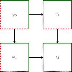
Figure 4.1: The interplay of Neumann corrections, solid line: no error, dashed line: error, densely-dotted line: correction

Let us start by defining $\psi_{0}$. It solves a reduced problem that can formally be found by comparing powers of $\varepsilon$ in the general approach (4.1). We have

$$(\boldsymbol{b}\cdot\nabla)\Delta\psi_{0}-c\Delta\psi_{0} =f\quad \mbox{ in }\Omega=(0,1)^{2},$$ (4.3a)

$$\psi_{0} =0 \mbox{ on }\Gamma=\partial\Omega,$$ (4.3b)

$$\partial_{\boldsymbol{n}}\psi_{0} =0 \mbox{ on }\Gamma_{-},$$ (4.3c)

where $\Gamma_{-}:=\{(x,y)\in\Gamma|-\boldsymbol{b}\cdot\boldsymbol{n}(x,y)<0\}$ is the inflow boundary. According to Proposition 2.21 the third-order problem (4.3) has a unique solution satisfying homogeneous Dirichlet conditions on the whole boundary $\Gamma$, and homogeneous Neumann conditions on the inflow boundary $\Gamma_{-}$ only. This is similar to the asymptotic expansions for second order problems as in [13].

Now the normal derivative of $\psi_{0}$ is in general non-zero on the outflow boundary. Thus, we correct these Neumann data by correction functions $v_{i}$ in $x$-direction and $w_{i}$ in $y$-direction. We recall our standing assumption of ${\boldsymbol{b}}>0$, the general case ${\boldsymbol{b}}=(b_{1},b_{2})$ with $b_{1}\cdot b_{2}\neq 0$ can be derived from the one with ${\boldsymbol{b}}>0$ by a change of coordinates. Using ${\boldsymbol{b}}>0$, we find the outflow boundary at $x=0$ and $y=0$. The layers occur at $x=0$ and $y=0$ as well.

We will now define the correction function for the layer at $x=0$. They can formally be derived with the help of the stretched variable $\xi$ defined by $\xi=\frac{x}{\varepsilon}$ and comparison of powers of $\varepsilon$ in the transformed differential operator $\tilde{L}$. We obtain $\tilde{L}$ expressed in terms of the variable $\xi$ and $y$ by a coordinate transformation

$$\tilde{L}\tilde{v}(\xi,y) =\varepsilon^{-3}\tilde{v}_{\xi\xi\xi\xi}+2\varepsilon^{-1}\tilde{v}_{\xi\xi yy}+\varepsilon\tilde{v}_{yyyy}+\varepsilon^{-3}b_{1}\tilde{v}_{\xi\xi\xi}+\varepsilon^{-1}b_{1}\tilde{v}_{\xi yy}+\varepsilon^{-2}b_{2}\tilde{v}_{\xi\xi y}+b_{2}\tilde{v}_{yyy}$$

$$\quad-\varepsilon^{-2}c\tilde{v}_{\xi\xi}-c\tilde{v}_{yy}$$

$$=\varepsilon^{-3}(\tilde{v}_{\xi}+b_{1}\tilde{v})_{\xi\xi\xi}+\varepsilon^{-2}(b_{2}\tilde{v}_{y}-c\tilde{v})_{\xi\xi}+\varepsilon^{-1}(2\tilde{v}_{\xi}+b_{1}\tilde{v})_{\xi yy}+(b_{2}\tilde{v}_{y}-c\tilde{v})_{yy}+\varepsilon\tilde{v}_{yyyy}.$$ (4.4)

Now the function $v$ is to correct the Neumann data. Thus, it has to fulfil the boundary conditions at $x=0$, that is $\xi=0$. Therefore, we consider the Neumann derivative in $x=0$ of the (formally) infinite sum (4.1) and make a comparison in the powers of $\varepsilon$. The last two sums are set to zero, because they do not have to correct anything. We get conditions on the functions $\psi_{i}$ and $\tilde{v}_{i}$, namely

$$\psi_{i,x}(0,y)=-\tilde{v}_{i+1,\xi}(0,y)$$ (4.5)

for correcting the contributions of $\psi_{i}$ to the Neumann data at $x=0$. The functions $\psi_{i}$ and $\tilde{v}_{i}$ act on different $\varepsilon$-levels because we consider the derivative of $\tilde{v}_{i}$ in $\xi$ and thus, we get an additional order of $\varepsilon$. Note that we do not correct the boundary conditions up to arbitrarily large values of $i$. We make use of this condition only for the considered finite number of indices. Additionally, the boundary correction functions are expected to be exponentially decaying away from the boundary. For this reason, we expand the domain of $\tilde{L}$ from $(0,\frac{1}{\varepsilon})\times(0,1)$ to $(0,\infty)\times(0,1)$.

Now, the boundary condition (4.5) shows that the contribution of $\psi_{0}$ will be corrected by $v_{1}$. Thus, $v_{0}$ has nothing to correct and therefore we set

$$\tilde{v}_{0}=0.$$

For $\tilde{v}_{1}$ the comparison of powers of $\varepsilon$ in (4.4) with $\tilde{L}\tilde{v}=0$ yields

$$\begin{split}\tilde{v}_{1,\xi\xi\xi\xi}+b_{1}\tilde{v}_{1,\xi\xi\xi}=-b_{2}\tilde{v}_{0,\xi\xi y}+c\tilde{v}_{0,\xi\xi}&=0\hskip 20.00003pt\mbox{ in }(0,\infty)\times(0,1),\\ \tilde{v}_{1,\xi}(0,y)=-\psi_{0,x}(0,y)\mbox{ and }\lim_{\xi\rightarrow\infty}\tilde{v}_{1}(\xi,y)&=0.\end{split}$$

This problem has constant coefficients and no derivatives in $y$. Therefore, it can be solved explicitly and has the solution

$$\tilde{v}_{1}(\xi,y)=\frac{\psi_{0,x}(0,y)}{b_{1}}\exp\{-b_{1}\xi\}\quad\text{ or }\quad v_{1}(x,y)=\frac{\psi_{0,x}(0,y)}{b_{1}}E_{1}(x).$$

Analogously, we obtain the correction function $\tilde{w}_{0}=0$ and $\tilde{w}_{1}(x,\eta)$ with the stretched variable $\eta=\frac{y}{\varepsilon}$ for the layer along $y=0$:

$$\tilde{w}_{1}(x,\eta)=\frac{\psi_{0,y}(x,0)}{b_{2}}\exp\{-b_{2}\eta\}\quad\text{ or }\quad w_{1}(x,y)=\frac{\psi_{0,y}(x,0)}{b_{2}}E_{2}(y).$$

Both boundary correction functions $v_{1}$ and $w_{1}$ introduce non-zero Dirichlet and Neumann contributions at the outflow-boundary. We correct the Neumann data by a corner correction function $z_{2}$ and the Dirichlet data by $\psi_{1}$. For the corner-correction function we apply the stretching of the coordinates in both directions and obtain formally the operator

$$\bar{L}\bar{z}(\xi,\eta)=\varepsilon^{-3}(\bar{z}_{\xi\xi\xi\xi}+2\bar{z}_{\xi\xi\eta\eta}+\bar{z}_{\eta\eta\eta\eta})+\varepsilon^{-3}(b_{1}(\bar{z}_{\xi\xi\xi}+\bar{z}_{\eta\eta\xi})+b_{2}(\bar{z}_{\xi\xi\eta}+\bar{z}_{\eta\eta\eta}))-\varepsilon^{-2}c(\bar{z}_{\xi\xi}+\bar{z}_{\eta\eta}).$$

Again, the correction function is to correct the Neumann data of $v$ along $y=0$ ($\eta=0$) and of $w$ along $x=0$ ($\xi=0$). Thus we have

$$\tilde{v}_{i,y}(\xi,0)=-\bar{z}_{i+1,\eta}(\xi,0)\quad\mbox{ and }\quad\tilde{w}_{i,x}(0,\eta)=-\bar{z}_{i+1,\xi}(0,\eta),$$

respectively. This time we obtain $\bar{z}_{0}=\bar{z}_{1}=0$ because they have nothing to correct. The corner-correction function $\bar{z}_{2}$ satisfies

$$\bar{\Delta}^{2}\bar{z}_{2}+(b\cdot\bar{\nabla})\bar{\Delta}\bar{z}_{2}=c\bar{\Delta}\bar{z}_{1} =0\hskip 60.00009pt\mbox{in }(0,\infty)\times(0,\infty),$$

$$\bar{z}_{2,\eta}(\xi,0)=-\tilde{v}_{1,y}(\xi,0)\mbox{ and }\bar{z}_{2,\xi}(0,\eta) =-\tilde{w}_{1,x}(0,\eta),$$

$$\lim_{\xi\rightarrow\infty}\bar{z}_{2}(\xi,\eta)=0\mbox{ and }\lim_{\eta\rightarrow\infty}\bar{z}_{2}(\xi,\eta) =0.$$

A solution can be found to be

$$\bar{z}_{2}(\xi,\eta)=-\frac{\psi_{0,xy}(0,0)}{b_{1}b_{2}}\exp\{-b_{1}\xi\}\exp\{-b_{2}\eta\}\quad\text{ or }\quad z_{2}(x,y)=-\frac{\psi_{0,xy}(0,0)}{b_{1}b_{2}}E_{1}(x)E_{2}(y).$$

As said before, the boundary-correction functions $v_{1}$ and $w_{1}$ introduce non-neglectable contributions in the Dirichlet data on $\Gamma_{+}:=\{(x,y)\in\Gamma:-{\boldsymbol{b}}\cdot\boldsymbol{n}(x,y)>0\}$. This will be corrected in the next step by $\psi_{1}$ satisfying the reduced problem

$$(\boldsymbol{b}\cdot\nabla)\Delta\psi_{1}-c\Delta\psi_{1} =-\Delta^{2}\psi_{0} \hskip 20.00003pt\mbox{in }\Omega=(0,1)^{2},$$

$$\psi_{1} =0 \hskip 20.00003pt\mbox{on }\Gamma_{-},$$

$$\partial_{\boldsymbol{n}}\psi_{1}(x,y) =0 \hskip 20.00003pt\mbox{on }\Gamma_{-},$$

$$\psi_{1}(0,y) =-v_{1}(0,y) \hskip 20.00003pty\in(0,1),$$

$$\psi_{1}(x,0) =-w_{1}(x,0) \hskip 20.00003ptx\in(0,1).$$

It can be checked that the conditions for existence of a unique solution, given in Proposition 2.21, are fulfilled.

Now the construction of problems for $v_{2}$ and $w_{2}$ follows the same pattern as the construction for $v_{1}$ and $w_{1}$, respectively. We get

$$\tilde{v}_{2}(\xi,y) =\left(\frac{\psi_{1,x}(0,y)}{b_{1}}-\frac{\alpha(y)}{b_{1}^{3}}-\frac{\alpha(y)\xi}{b_{1}^{2}}\right)\exp\{-b_{1}\xi\},$$

$$\text{ that is }v_{2}(x,y) =\left(\frac{\psi_{1,x}(0,y)}{b_{1}}-\frac{\alpha(y)}{b_{1}^{3}}-\frac{\alpha(y)x}{b_{1}^{2}\varepsilon}\right)E_{1}(x)$$

$$\mbox{with }\alpha(y) =-b_{2}\psi_{0,xy}(0,y)+c\psi_{0,x}(0,y)$$

and

$$\tilde{w}_{2}(x,\eta) =\left(\frac{\psi_{1,y}(x,0)}{b_{2}}-\frac{\beta(x)}{b_{2}^{3}}-\frac{\beta(x)\eta}{b_{2}^{2}}\right)\exp\{-b_{2}\eta\},$$

$$\text{ that is }w_{2}(x,y) =\left(\frac{\psi_{1,y}(x,0)}{b_{2}}-\frac{\beta(x)}{b_{2}^{3}}-\frac{\beta(x)y}{b_{2}^{2}\varepsilon}\right)E_{2}(y)$$

$$\mbox{with }\beta(x) =-b_{1}\psi_{0,xy}(x,0)+c\psi_{0,y}(x,0).$$

The function $$\bar{z}_{3}$$ has to fulfil the following problem:

$$\bar{\Delta}^{2}\bar{z}_{3}+(b\cdot\bar{\nabla})\bar{\Delta}\bar{z}_{3}=c\bar{\Delta}\bar{z}_{2} =-\frac{c(b_{1}^{2}+b_{2}^{2})}{b_{1}b_{2}}\psi_{0,xy}(0,0)\exp\{-b_{1}\xi\}\exp\{-b_{2}\eta\} \mbox{in }(0,\infty)\times(0,\infty),$$

$$\bar{z}_{3,\eta}(\xi,0) =-\tilde{v}_{2,y}(\xi,0)\quad\mbox{and}\quad\bar{z}_{3,\xi}(0,\eta)=-\tilde{w}_{2,x}(0,\eta),$$

$$\lim_{\xi\rightarrow\infty}\bar{z}_{3}(\xi,\eta) =0\quad\mbox{and}\quad\lim_{\eta\rightarrow\infty}\bar{z}_{3}(\xi,\eta)=0.$$

We make the ansatz

$${z}_{3}(\xi,\eta)=(\omega_{1}+\omega_{2}\xi+\omega_{3}\eta)\exp\{-b_{1}\xi\}\exp\{-b_{2}\eta\}$$

with unknown constants $\omega_{1},\omega_{2},\omega_{3}$. With this ansatz, we get only a solution if the compatibility condition

$$({\boldsymbol{b}}\cdot\nabla)\psi_{0,xy}(0,0)-c\psi_{0,xy}(0,0)=0$$ (4.6)

holds true. Then, the solution is given by

$$\bar{z}_{3}(\xi,\eta)=(\omega_{1}+\omega_{2}\xi+\omega_{3}\eta)\exp\{-b_{1}\xi\}\exp\{-b_{2}\eta\}\quad\text{ or }\quad z_{3}(x,y)=\left(\omega_{1}+\omega_{2}\frac{x}{\varepsilon}+\omega_{3}\frac{y}{\varepsilon}\right)E_{1}(x)E_{2}(y)$$

with

$$\omega_{1} =\frac{-b_{1}b_{2}\psi_{1,xy}(0,0)+b_{1}\psi_{0,xyy}(0,0)+b_{2}\psi_{0,xxy}(0,0)}{b_{1}^{2}b_{2}^{2}},$$

$$\omega_{2} =\frac{\psi_{0,xxy}(0,0)}{b_{1}b_{2}}\quad\mbox{and}\quad\omega_{3}=\frac{\psi_{0,xyy}(0,0)}{b_{1}b_{2}}.$$

Without the explicit ansatz for $z_{3}$ we also get several compatibility conditions, which follow from the differential equation itself and the boundary conditions, warranting $z_{3}$ to be continuous in the corner (0,0).

Now $z_{2}$ introduces non-neglectable contributions in the Dirichlet data on $\Gamma_{+}$. Thus for the next step, $\psi_{2}$ has to correct the Dirichlet data of $v_{2},w_{2}$ and $z_{2}$. We consider the equation

$$(\boldsymbol{b}\cdot\nabla)\Delta\psi_{2}-c\Delta\psi_{2} =-\Delta^{2}\psi_{1} \hskip 20.00003pt\mbox{in }\Omega=(0,1)^{2},$$

$$\psi_{2} =0 \hskip 20.00003pt\mbox{on }\Gamma_{-},$$

$$\partial_{\boldsymbol{n}}\psi_{2} =0 \hskip 20.00003pt\mbox{on }\Gamma_{-},$$

$$\psi_{2}(0,y) =-v_{2}(0,y)-w_{2}(0,y)-z_{2}(0,y) \hskip 20.00003pty\in(0,1),$$

$$\psi_{2}(x,0) =-v_{2}(x,0)-w_{2}(x,0)-z_{2}(x,0) \hskip 20.00003ptx\in(0,1).$$

We again have to check the conditions of Proposition 2.21. Therefore, we have to verify, whether the following equations hold

$$-v_{2}(0,1)-w_{2}(0,1)-z_{2}(0,1) =0,$$ (4.7a)

$$-v_{2}(1,0)-w_{2}(1,0)-z_{2}(1,0) =0,$$ (4.7b)

$$-v_{2,y}(0,1)-w_{2,y}(0,1)-z_{2,y}(0,1) =0,$$ (4.7c)

$$-v_{2,x}(1,0)-w_{2,x}(1,0)-z_{2,x}(1,0) =0.$$ (4.7d)

We begin with equation (4.7a):

$$v_{2}(0,1) +w_{2}(0,1)+z_{2}(0,1)$$

$$=\frac{\psi_{1,x}(0,1)}{b_{1}}-\frac{\alpha(1)}{b_{1}^{3}}+\left(\frac{\psi_{1,y}(0,0)}{b_{2}}-\frac{\beta(0)}{b_{2}^{3}}-\frac{\beta(0)}{b_{2}^{2}\varepsilon}\right)E_{2}(1)-\frac{\psi_{0,xy}(0,0)}{b_{1}b_{2}}E_{2}(1)$$

$$=\left(-\frac{2}{b_{1}b_{2}}+\frac{b_{1}}{b_{2}^{3}}+\frac{b_{1}}{b_{2}^{2}\varepsilon}\right)\psi_{0,xy}(0,0)E_{2}(1)=0.$$

This is zero, if

$$\psi_{0,xy}(0,0)=0.$$ (4.8)

Equation (4.7b) yields

$$v_{2}(1,0) +w_{2}(1,0)+z_{2}(1,0)$$

$$=\left(\frac{\psi_{1,x}(0,0)}{b_{1}}-\frac{\alpha(0)}{b_{1}^{3}}-\frac{\alpha(0)}{b_{1}^{2}\varepsilon}\right)E_{1}(1)+\frac{\psi_{1,y}(1,0)}{b_{2}}-\frac{\beta(1)}{b_{2}^{3}}-\frac{\psi_{0,xy}(0,0)}{b_{1}b_{2}}E_{1}(1)$$

$$=\left(-\frac{2}{b_{1}b_{2}}+\frac{b_{2}}{b_{1}^{3}}+\frac{b_{2}}{b_{1}^{2}\varepsilon}\right)\psi_{0,xy}(0,0)E_{1}(1)=0$$

and also gives condition (4.8). Let us continue with equation (4.7c):

$$v_{2,y}(0,1) +w_{2,y}(0,1)+z_{2,y}(0,1)$$

$$=\frac{\psi_{1,xy}(0,1)}{b_{1}}-\frac{\alpha_{y}(1)}{b_{1}^{3}}+\left(\frac{-b_{2}}{\varepsilon}\left(\frac{\psi_{1,y}(0,0)}{b_{2}}-\frac{\beta(0)}{b_{2}^{3}}-\frac{\beta(0)}{b_{2}^{2}\varepsilon}\right)-\frac{\beta(0)}{b_{2}^{2}\varepsilon}\right)E_{2}(1)+\frac{\psi_{0,xy}(0,0)}{b_{1}}E_{2}(1)$$

$$\overset{\eqref{eq:compcond2}}{\underset{}{=}}\frac{\psi_{1,xy}(0,1)}{b_{1}}-\frac{\alpha_{y}(1)}{b_{1}^{3}}-\frac{\psi_{1,y}(0,0)}{\varepsilon}E_{2}(1)$$

$$=\frac{b_{2}\psi_{0,xyy}(0,1)}{b_{1}^{3}}=0.$$

Analogously, we get for equation (4.7d)

$$v_{2,x}(1,0)+w_{2,x}(1,0)+z_{2,x}(1,0)=\frac{b_{1}\psi_{0,xxy}(1,0)}{b_{2}^{3}}=0.$$

Thus we obtain the additional conditions

$$\psi_{0,xyy}(0,1)=0\quad\mbox{and}\quad\psi_{0,xxy}(1,0)=0.$$ (4.9)

If the conditions (4.8) and (4.9) are violated, Proposition 2.21 is not applicable. Hence, it is unclear, whether a solution $\psi_{2}$ exists. Condition (4.8) implies that $z_{2}=0$.

Remark 4.1.

From the conditions (4.9) we get conditions on $f$, namely $f(0,1)=0$ and $f(1,0)=0$. This follows by extension of the differential equation for $\psi_{0}$ to the boundary. Furthermore, if $b_{1}=b_{2}$, condition (4.6) implies that $f(0,0)=0$.

The construction of $v_{3}$ and $w_{3}$ follows the same pattern as those for $v_{1},v_{2},w_{1}$ and $w_{2}$. The structure of the solutions is of the form

$$\tilde{v}_{3}(\xi,y)=\widetilde{P}_{2}(\xi,y)\exp\{-b_{1}\xi\} \quad\text{ or }\quad v_{3}(x,y)=\widetilde{P}_{2}\left(\frac{x}{\varepsilon},y\right)E_{1}(x),$$

$$\tilde{w}_{3}(x,\eta)=\widetilde{Q}_{2}(x,\eta)\exp\{-b_{2}\eta\} \quad\text{ or }\quad w_{3}(x,y)=\widetilde{Q}_{2}\left(x,\frac{y}{\varepsilon}\right)E_{2}(y),$$

where $\widetilde{P}_{2}$ is a polynomial of second order in the first variable and $\widetilde{Q}_{2}$ a polynomial of second order in the second variable. To continue the expansion with higher order terms of $\epsilon$ in the same manner results in more compatibility conditions. So, we stop the classical asymptotic expansion here. We add functions $\tilde{v}_{4},\tilde{w}_{4}$ and $\bar{z}_{4}$ not correcting the boundary layers, but modifying the right hand-side of the residual. We want them to satisfy:

$$\tilde{v}_{4,\xi\xi\xi\xi}+b_{1}\tilde{v}_{4,\xi\xi\xi} =-b_{2}\tilde{v}_{3,\xi\xi y}+c\tilde{v}_{3,\xi\xi}-2\tilde{v}_{2,\xi\xi yy}-b_{1}\tilde{v}_{2,\xi yy}-b_{2}\tilde{v}_{1,yyy}+c\tilde{v}_{1,yy},\quad\mbox{in }(0,\infty)\times(0,1),$$

$$\tilde{v}_{4,\xi}(0,y) =0,\,\mbox{in }(0,1),$$

$$\lim_{\xi\rightarrow\infty}\tilde{v}_{4}(\xi,y) =0,\,\mbox{in }(0,1),$$

$$\tilde{w}_{4,\eta\eta\eta\eta}+b_{2}\tilde{w}_{4,\eta\eta\eta} =-b_{1}\tilde{w}_{3,x\eta\eta}+c\tilde{w}_{3,\eta\eta}-2\tilde{w}_{2,xx\eta\eta}-b_{2}\tilde{w}_{2,xx\eta}-b_{1}\tilde{w}_{1,xxx}+c\tilde{w}_{1,xx},\quad\mbox{in }(0,1)\times(0,\infty),$$

$$\tilde{w}_{4,\eta}(x,0) =0,\,\mbox{in }(0,1),$$

$$\lim_{\eta\rightarrow\infty}\tilde{w}_{4}(x,\eta) =0,\,\mbox{in }(0,1),$$

$$\bar{\Delta}^{2}\bar{z}_{4}+(b\cdot\bar{\nabla})\bar{\Delta}\bar{z}_{4} =c\bar{\Delta}\bar{z}_{3}.$$

The boundary data of $\bar{z}_{4}$ only have to be bounded by a constant and need not to correct other data, thus we have some freedem in the choice for $\bar{z}_{4}$. We get

$$\tilde{v}_{4}(\xi,y)=\widetilde{P}_{3}(\xi,y)\exp\{-b_{1}\xi\} \quad\text{ or }\quad v_{3}(x,y)=\widetilde{P}_{3}\left(\frac{x}{\varepsilon},y\right)E_{1}(x),$$

$$\tilde{w}_{4}(x,\eta)=\widetilde{Q}_{3}(x,\eta)\exp\{-b_{2}\eta\} \quad\text{ or }\quad w_{3}(x,y)=\widetilde{Q}_{3}\left(x,\frac{y}{\varepsilon}\right)E_{2}(y),$$

where $\tilde{P}_{3}$ is a polynomial of third order in the first variable and $\tilde{Q}_{3}$ a polynomial of third order in the second variable. The function $z_{4}$ is of the structure

$$\bar{z}_{4}(\xi,\eta)=\bar{R}_{2}(\xi,\eta)\exp\{-b_{1}\xi\}\exp\{-b_{2}\eta\}\quad\text{ or }\quad z_{4}(x,y)=\bar{R}_{2}\left(\frac{x}{\varepsilon},\frac{y}{\varepsilon}\right)E_{1}(x)E_{2}(y),$$

where $\bar{R}$ is a polynomial of second order in both variables.

4.2 Estimating the residual

Consider now the approximation $\Psi$ of $\psi$ given by

$$\Psi=\sum_{i=0}^{2}\varepsilon^{i}\psi_{i}+\sum_{i=1}^{4}\varepsilon^{i}v_{i}+\sum_{i=1}^{4}\varepsilon^{i}w_{i}+\sum_{i=2}^{4}\varepsilon^{i}z_{i},$$

with the functions given before. Furthermore, let $R=\psi-\Psi$ be the residual of the solution of problem (1.1) and its approximation $\Psi$. We now estimate the residual $R$ with the help of Theorem 3.3. Let us start with some lemmas. In all the lemmas, it is implicitly assumed that the compatibility conditions (4.6), (4.8) and (4.9) are fulfilled. We also recall our standing assumption on the solutions to be sufficiently smooth.

Lemma 4.2.

For the residual $R$ holds

$$\|LR\|_{L^{2}(\Omega)}\leq C\varepsilon^{5/2}.$$ (4.10)

Proof.

Let us start by computing

$$LR =L(\psi-\psi_{0}-\varepsilon\psi_{1}-\varepsilon^{2}\psi_{2}-\varepsilon v_{1}-\varepsilon^{2}v_{2}-\varepsilon^{3}v_{3}-\varepsilon^{4}v_{4}-\varepsilon w_{1}-\varepsilon^{2}w_{2}-\varepsilon^{3}w_{3}-\varepsilon^{4}w_{4}$$

$$\quad-\varepsilon^{2}z_{2}-\varepsilon^{3}z_{3}-\varepsilon^{4}z_{4})$$

$$=L(\psi-\psi_{0}-\varepsilon\psi_{1}-\varepsilon^{2}\psi_{2})-L(\varepsilon v_{1}+\varepsilon^{2}v_{2}+\varepsilon^{3}v_{3}+\varepsilon^{4}v_{4})$$

$$\quad-L(\varepsilon w_{1}+\varepsilon^{2}w_{2}+\varepsilon^{3}w_{3}+\varepsilon^{4}w_{4})-L(\varepsilon^{2}z_{2}+\varepsilon^{3}z_{3}+\varepsilon^{4}z_{4}).$$ (4.11)

We obtain for the first term of (4.11)

$$L(\psi-\psi_{0}-\varepsilon\psi_{1}-\varepsilon^{2}\psi_{2}) =f-f+\varepsilon\Delta^{2}\psi_{0}-\varepsilon\Delta^{2}\psi_{0}+\varepsilon^{2}\Delta^{2}\psi_{1}-\varepsilon^{2}\Delta^{2}\psi_{1}+\varepsilon^{3}\Delta^{2}\psi_{2}$$

$$=\varepsilon^{3}\Delta^{2}\psi_{2}.$$

For the second term of (4.11) we have

$$L(\varepsilon v_{1}+\varepsilon^{2}v_{2}+\varepsilon^{3}v_{3}+\varepsilon^{4}v_{4}) =\tilde{L}(\varepsilon\tilde{v}_{1}+\varepsilon^{2}\tilde{v}_{2}+\varepsilon^{3}\tilde{v}_{3}+\varepsilon^{4}\tilde{v}_{4})$$

$$=\varepsilon^{2}\left((\tilde{v}_{1,yy}+b_{2}\tilde{v}_{2,y}-c\tilde{v}_{2}+2\tilde{v}_{3,\xi\xi}+b_{1}\tilde{v}_{3,\xi})_{yy}+(b_{2}\tilde{v}_{4,y}-c\tilde{v}_{4})_{\xi\xi}\right)$$

$$\quad+\varepsilon^{3}(\tilde{v}_{2,yy}+b_{2}\tilde{v}_{3,y}-c\tilde{v}_{3}+2\tilde{v}_{4,\xi\xi}+b_{1}\tilde{v}_{4,\xi})_{yy}$$

$$\quad+\varepsilon^{4}(\tilde{v}_{3,yy}+b_{2}\tilde{v}_{4,y}-c\tilde{v}_{4})_{yy}+\varepsilon^{5}\tilde{v}_{4,yyyy}.$$

The third term of (4.11) can be rewritten analogously. Finally, the remaining term in (4.11) is

$$L(\varepsilon^{2}z_{2}+\varepsilon^{3}z_{3}+\varepsilon^{4}z_{4}) =\bar{L}(\varepsilon^{2}\bar{z_{2}}+\varepsilon^{3}\bar{z}_{3}+\varepsilon^{4}\bar{z}_{4})$$

$$=-\varepsilon^{2}c\bar{\Delta}\bar{z}_{4}.$$

Thus, we obtain with some functions $g_{1},\,g_{2},\,g_{3}$ that are bounded independently of $\varepsilon$

$$LR(x,y)=\varepsilon^{3}\Delta^{2}\psi_{2}(x,y)+\varepsilon^{2}(g_{1}(y)E_{1}(x)+g_{2}(x)E_{2}(y)+g_{3}(x,y)E_{1}(x)E_{2}(y))\quad(0\leq x,y\leq 1),$$

which yields (4.10). $\Box$

Lemma 4.3.

The residual $R$ can be bounded on the boundary $\Gamma=\partial\Omega$ by

$$\|R\|_{L^{\infty}(\Gamma)}\leq C\varepsilon^{3}.$$ (4.12)

Its tangential derivative $\partial_{t}$ is bounded on $\partial\Omega$ by

$$\|\partial_{t}R\|_{L^{\infty}(\Gamma)}\leq C\varepsilon^{2}.$$ (4.13)

Proof.

We will give details only for some of the terms occuring in the expression for $R$ as the estimates for the others follow the same rationale. Let us start out with

$$R(1,y) =\psi(1,y)-\psi_{0}(1,y)-\varepsilon\psi_{1}(1,y)-\varepsilon^{2}\psi_{2}(1,y)$$

$$\quad-\varepsilon(v_{1}(1,y)+w_{1}(1,y))-\varepsilon^{2}(v_{2}(1,y)+w_{2}(1,y)+z_{2}(1,y))$$

$$\quad-\varepsilon^{3}(v_{3}(1,y)+w_{3}(1,y)+z_{3}(1,y))-\varepsilon^{4}(v_{4}(1,y)+w_{4}(1,y)+z_{4}(1,y))$$

The first four terms of $R(1,y)$ are zero, because these functions fulfil homogeneous Dirichlet boundary conditions.

The correction terms with index 1 yield

$$v_{1}(1,y)+w_{1}(1,y)=\frac{\psi_{0,x}(0,y)}{b_{1}}E_{1}(1)+\frac{\psi_{0,y}(1,0)}{b_{2}}E_{2}(0)=\frac{\psi_{0,x}(0,y)}{b_{1}}E_{1}(1)$$

because $\psi_{0,y}(1,0)=0$ due to homogeneous Dirichlet boundary conditions of $\psi_{0}$. The factor $E_{1}(1)$ is exponentially small in $\varepsilon$ and can therefore be bounded by an arbitrary power of $\varepsilon$. For the corrections with index 2 we have

$$w_{2}(1,y)=\left(\frac{\psi_{1,y}(1,0)}{b_{2}}-\frac{\beta(1)}{b_{2}^{3}}-\frac{\beta(1)y}{b_{2}^{2}\varepsilon}\right)E_{2}(y)=0$$

because $\beta(1)=0$ due to $\psi_{0,xy}(1,0)=0$ and $\psi_{1,y}(1,0)=0$ due to homogeneous Dirichlet boundary conditions of $\psi_{1}$, and

$$v_{2}(1,y)+z_{2}(1,y)=v_{2}(1,y)=\left(\frac{\psi_{1,x}(0,y)}{b_{1}}-\frac{\alpha(y)}{b_{1}^{3}}-\frac{\alpha(y)}{b_{1}^{2}\varepsilon}\right)E_{1}(1).$$

We obtain for the corrections with index 3

$$v_{3}(1,y)+z_{3}(1,y)=\widetilde{P}_{2}\left(x=\frac{1}{\varepsilon},y\right)E_{1}(1)+\bar{R}_{1}\left(x=\frac{1}{\varepsilon},\frac{y}{\varepsilon}\right)E_{1}(1)E_{2}(y).$$

Finally,

$$w_{3}(1,y)=\widetilde{Q}_{2}\left(1,\frac{y}{\varepsilon}\right)E_{2}(y)$$

is bounded by a constant due to $P_{2}(t)\mathrm{e}^{-t}\leq C$ for all $t$, where $P_{2}$ is a polynomial of order $2$. The corrections with index 4 contribute similar bounds as an analogous argument shows. Combining the terms discussed so far, we obtain with some function $g$, bounded independently of $\varepsilon$, and polynomials $P_{2},P_{3},$

$$R(1,y)=\varepsilon g(y)E_{1}(1)+\left(\varepsilon^{3}P_{2}\left(\frac{y}{\varepsilon}\right)+\varepsilon^{4}P_{3}\left(\frac{y}{\varepsilon}\right)\right)E_{2}(y),\quad(0\leq y\leq 1).$$

Thus, the $L^{\infty}$-norm over this part of the boundary is bounded by

$$\|R(1,\cdot)\|_{L^{\infty}(0,1)}\leq C\varepsilon^{3}.$$

Let us take a look at the outflow boundary at $x=0$. Here, we do not have an arbitrarily small factor $E_{1}(1)$ in our estimates. We start with

$$R(0,y) =\psi(0,y)-\psi_{0}(0,y)-\varepsilon\psi_{1}(0,y)-\varepsilon^{2}\psi_{2}(0,y)$$

$$\quad-\varepsilon(v_{1}(0,y)+w_{1}(0,y))-\varepsilon^{2}(v_{2}(0,y)+w_{2}(0,y)+z_{2}(0,y))$$

$$\quad-\varepsilon^{3}(v_{3}(0,y)+w_{3}(0,y)+z_{3}(0,y))-\varepsilon^{4}(v_{4}(0,y)+w_{4}(0,y)+z_{4}(0,y)).$$

The first two terms are zero due to the imposed Dirichlet conditions. By definition of $\psi_{1}$ and $\psi_{2}$ we have

$$\psi_{1}(0,y) =-v_{1}(0,y),$$

$$\psi_{2}(0,y) =-v_{2}(0,y)-w_{2}(0,y)-z_{2}(0,y).$$

Employing the fact that $w_{1}(0,y)$ is zero since $\psi_{0}$ satisfies homogeneous Dirichlet conditions and, hence, $\psi_{0,y}(0,0)=0$, we get

$$R(0,y) =-\varepsilon^{3}(v_{3}(0,y)+w_{3}(0,y)+z_{3}(0,y))-\varepsilon^{4}(v_{4}(0,y)+w_{4}(0,y)+z_{4}(0,y)).$$

We obtain with the same methods as above for some function $h$ bounded independently of $\varepsilon$ and polynomials $P_{2},P_{3}$,

$$R(0,y)=\varepsilon^{3}\left(h(y)+\left(P_{2}\left(\frac{y}{\varepsilon}\right)+\varepsilon P_{3}\left(\frac{y}{\varepsilon}\right)\right)E_{2}(y)\right)\quad(0\leq y\leq 1).$$

Thus, the $L^{\infty}$-norm of this part of the boundary is also bounded by

$$\|R(0,\cdot)\|_{L^{\infty}(0,1)}\leq C\varepsilon^{3}.$$

On the remaining boundaries we use similar ideas and eventually obtain (4.12).

For the tangential derivative we estimate $R_{y}(0,y)$ and $R_{y}(1,y)$: We obtain

$$\|R_{y}(0,\cdot)\|_{L^{\infty}(0,1)}\leq C\varepsilon^{2}\quad\mbox{and}\quad\|R_{y}(1,\cdot)\|_{L^{\infty}(0,1)}\leq C\varepsilon^{2}$$

due to $E_{2,y}(y)=-\frac{b_{2}}{\varepsilon}E_{2}(y)$. On the other boundaries we apply the same techniques and conclude (4.13). $\Box$

Lemma 4.4.

The normal derivative of $R$ on the boundary $\partial\Omega$ can be estimated by

$$\|\partial_{\boldsymbol{n}}R\|_{L^{\infty}(\Gamma)}\leq C\varepsilon^{3}\mbox{ and }\|\partial_{\boldsymbol{n}}R\|_{L^{2}(\Gamma)}\leq C\varepsilon^{7/2}.$$ (4.14)

Proof.

Again, we only exemplify the method of proof. The terms not discussed are estimated using the same techniques. Let us start out with $R(1,y)$. Here, we have

$$R_{x}(1,y) =\psi_{x}(1,y)-\psi_{0,x}(1,y)-\varepsilon\psi_{1,x}(1,y)-\varepsilon^{2}\psi_{2,x}(1,y)$$

$$\quad-\varepsilon(v_{1,x}(1,y)+w_{1,x}(1,y))-\varepsilon^{2}(v_{2,x}(1,y)+w_{2,x}(1,y)+z_{2,x}(1,y))$$

$$\quad-\varepsilon^{3}(v_{3,x}(1,y)+w_{3,x}(1,y)+z_{3,x}(1,y))-\varepsilon^{4}(v_{4,x}(1,y)+w_{4,x}(1,y)+z_{4,x}(1,y)).$$

Now,

$$\psi_{x}(1,y)-\psi_{0,x}(1,y)-\varepsilon\psi_{1,x}(1,y)-\varepsilon^{2}\psi_{2,x}(1,y)=0$$

due to the homogeneous Neumann boundary conditions at this boundary of the functions $\psi,\psi_{0},\psi_{1}$ and $\psi_{2}$. For the next terms we have

$$v_{1,x}(1,y)+w_{1,x}(1,y) =-\frac{\psi_{0,x}(1,y)}{\varepsilon}E_{1}(1)+\frac{\psi_{0,xy}(1,y)}{b_{2}}E_{2}(y)$$

$$=-\frac{\psi_{0,x}(1,y)}{\varepsilon}E_{1}(1)$$

because $\psi_{0}$ satisfies homogeneous Neumann boundary condition along $x=1$ and, hence, its $y$-derivative is zero. The terms with index 2 are

$$w_{2,x}(1,y) =\left(\frac{\psi_{1,xy}(1,0)}{b_{2}}-\frac{\beta_{x}(1)}{b_{2}^{3}}-\frac{\beta_{x}(1)y}{b_{2}^{2}\varepsilon}\right)E_{2}(y)$$

$$=\frac{b_{1}\psi_{0,xxy}(1,0)}{b_{2}^{3}}\left(1+\frac{b_{2}y}{\varepsilon}\right)E_{2}(y)=0,$$

due to the compatibility condition (4.9), and

$$v_{2,x}(1,y)+z_{2,x}(1,y)=-\frac{b_{1}}{\varepsilon}\left(\frac{\psi_{1,y}(1,0)}{b_{1}}-\frac{\alpha(y)}{b_{1}^{3}}-\frac{\alpha(y)}{b_{1}^{2}\varepsilon}\right)E_{1}(1).$$

The terms with index 3 contribute

$$v_{3,x}(1,y)+z_{3,x}(1,y) =\left(\tilde{P}_{2,x}\left(\frac{1}{\varepsilon},y\right)-\frac{b_{1}}{\varepsilon}\tilde{P}_{2}\left(\frac{1}{\varepsilon},y\right)\right.$$

$$\quad\left.+\frac{w_{2}}{\varepsilon}E_{2}(y)-\frac{b_{1}}{\varepsilon}\left(\omega_{1}+\omega_{2}\frac{1}{\varepsilon}+\omega_{3}\frac{y}{\varepsilon}\right)E_{2}(y)\right)E_{1}(1)$$

and

$$w_{3,x}(1,y)=\tilde{Q}_{2,x}\left(1,\frac{y}{\varepsilon}\right)E_{2}(y)$$

which is bounded by a constant due to $P_{2}(t)\mathrm{e}^{-t}\leq C$ for all $t$, where $P_{2}$ is a polynomial of order $2$. The same arguments apply to the correction functions with index 4. Combining all these terms, we have for some function $g$ bounded independently of $\varepsilon$ and constants $c_{7},c_{8}$ and $c_{9}$ independent of $\varepsilon$

$$R_{x}(1,y)=g(y)E_{1}(1)+\varepsilon^{3}\left(c_{7}+c_{8}\left(\frac{y}{\varepsilon}\right)+c_{9}\left(\frac{y}{\varepsilon}\right)^{2}\right)E_{2}(y).$$

Thus, we obtain

$$\|R_{x}(1,\cdot)\|_{L^{\infty}(0,1)}\leq C\varepsilon^{3}\quad\mbox{and}\quad\|R_{x}(1,\cdot)\|_{L^{2}(0,1)}\leq C\varepsilon^{7/2}.$$

On the outflow boundary at $x=0$ we have

$$R_{x}(0,y) =\psi_{x}(0,y)-\psi_{0,x}(0,y)-\varepsilon\psi_{1,x}(0,y)-\varepsilon^{2}\psi_{2,x}(0,y)$$

$$\quad-\varepsilon(v_{1,x}(0,y)+w_{1,x}(0,y))-\varepsilon^{2}(v_{2,x}(0,y)+w_{2,x}(0,y)+z_{2,x}(0,y)$$

$$\quad-\varepsilon^{3}(v_{3,x}(0,y)+w_{3,x}(0,y)+z_{3,x}(0,y))-\varepsilon^{4}(v_{4,x}(0,y)+w_{4,x}(0,y)+z_{4,x}(0,y)).$$

The first term is zero and the next terms cancel with their corresponding layer-correction functions. So far, we have

$$R_{x}(0,y)=-\varepsilon^{3}w_{3,x}(0,y)-\varepsilon^{4}(v_{4,x}(0,y)+w_{4,x}(0,y)+z_{4,x}(0,y)).$$

The remaining terms are not vanishing and we have for some function $h$ bounded independently of $\varepsilon$ and constants $c_{10},c_{11}$ and $c_{12}$ independent of $\varepsilon$

$$R_{x}(0,y)=\varepsilon^{4}h(y)+\varepsilon^{3}\left(c_{10}+c_{11}\left(\frac{y}{\varepsilon}\right)+c_{12}\left(\frac{y}{\varepsilon}\right)^{2}\right)E_{2}(y).$$

Thus, we obtain again

$$\|R_{x}(0,\cdot)\|_{L^{\infty}(0,1)}\leq C\varepsilon^{3}\quad\mbox{and}\quad\|R_{x}(0,\cdot)\|_{L^{2}(0,1)}\leq C\varepsilon^{7/2}.$$

The normal derivative on the other sides can be estimated similarly and we obtain (4.14). $\Box$

We summarize the results obtained so far in the next proposition. Recall that we assumed sufficiently smooth solutions to be existent.

Proposition 4.5.

Assume the compatibility conditions (4.6), (4.8) and (4.9) to be satisfied. We consider the approximation of $\psi$ given by

$$\Psi=\sum_{i=0}^{2}\varepsilon^{i}\psi_{i}+\sum_{i=1}^{4}\varepsilon^{i}v_{i}+\sum_{i=1}^{4}\varepsilon^{i}w_{i}+\sum_{i=2}^{4}\varepsilon^{i}z_{i}.$$

Then, the residual $R=\psi-\Psi$ can be estimated by

$$\|R\|_{L^{\infty}(\Omega)}\leq C\varepsilon^{3/2}\quad\mbox{and}\quad\|R\|_{H^{1}(\Omega)}\leq C\varepsilon^{3/2}.$$

Proof.

We make use of Theorem 3.3. For this, using Lemmas 4.2, 4.3, 4.4, we are left with an estimate of the $C^{1/2}$-norm on $\Gamma$ of $R$. But, with the help of the estimates in both the $C^{1}$- and $L^{\infty}$-norm it follows that

$$\|R\|_{C^{1/2}(\Gamma)}\leq C\varepsilon^{5/2}.$$

Hence, the assertion eventually follows from Theorem 3.3. $\Box$

Theorem 4.6.

Assume the compatibility conditions (4.6), (4.8) and (4.9) to be satisfied. Then the solution $\psi$ of (1.1) can be decomposed in a regular part $S$ and two layer parts in the following form:

$$\psi(x,y)=S(x,y)+\varepsilon H(x,y)E_{1}(x)+\varepsilon I(x,y)E_{2}(y),\quad(0\leq x,y\leq 1)$$

where the functions $S,H$ and $I$ are independently bounded of $\varepsilon$.

Proof.

The result follows from the asymptotic expansion which was done in this section. Proposition 4.5 yields that the residual $R$ is small enough and thus, it can be incorporated into the smooth part $S$ due to the structure of the layer correcting terms. The corner layer parts $z_{3}$ and $z_{4}$ are also incorporated into the smooth part. $\Box$

Remark 4.7.

The layers of $\psi$ are so-called weak layers. If we look at $\psi-S$, with $S$ being given by Theorem 4.6, we obtain

$$\|\psi-S\|_{L^{\infty}(\Omega)}\leq C\varepsilon,$$

but

$$\|\nabla(\psi-S)\|_{L^{\infty}(\Omega)}\leq C,$$

that is the layers are visible in the first derivative for $\varepsilon\to 0$.

4.3 Asymptotic expansion without compatibility conditions

With the rationale presented, we have seen that an asymptotic expansion of arbitrary order is possible upon imposing certain compatibility conditions. In fact, for the construction of $\psi_{2}$ we needed (4.8) and (4.9) to be satisfied. We make now an asymptotic expansion without any compatibility conditions and demonstrate that we will lose an $\varepsilon$-order in the estimates of the residual $R$, while we keep in mind that we assume the solutions occuring to be sufficiently smooth.

We keep the construction of the functions $\psi_{0},\psi_{1},v_{1},w_{1},v_{2},w_{2}$ and $z_{2}$. In the next step, we formally set $\psi_{2}=0$. This implies that we impose homogeneous boundary conditions for $v_{3}$ and $w_{3}$. For $z_{3}$ we choose an arbitrary, exponentially decaying function that fulfils a corner-correction type problem, given by

$$\bar{\Delta}^{2}\bar{z}_{3}+(b\cdot\bar{\nabla})\bar{\Delta}\bar{z}_{3} =c\bar{\Delta}\bar{z}_{2}$$

$$=-\frac{c\psi_{0,xy}(0,0)\exp\{-b_{1}\xi\}\exp\{-b_{2}\eta\}(b_{1}^{2}+b_{2}^{2})}{b_{1}b_{2}}\,\hskip 20.00003pt\mbox{in }(0,\infty)\times(0,\infty).$$

Its boundary data only have to be bounded by a constant and need not to correct other data, thus we have some freedom in choosing $\bar{z}_{3}$. We take

$$z_{3}(x,y)=\frac{c\psi_{0,xy}(0,0)}{b_{1}b_{2}(b_{1}+b_{2})}\left(\frac{x}{\varepsilon}+\frac{y}{\varepsilon}\right)E_{1}(x)E_{2}(y).$$

Next, we consider an approximation $\Psi^{\textnormal{new}}$ of $\psi$ given by

$$\Psi^{\textnormal{new}}=\psi_{0}+\varepsilon\psi_{1}+\varepsilon v_{1}+\varepsilon^{2}v_{2}+\varepsilon^{3}v_{3}+\varepsilon w_{1}+\varepsilon^{2}w_{2}+\varepsilon^{3}w_{3}+\varepsilon^{2}z_{2}+\varepsilon^{3}z_{3}.$$

Following the strategies exemplified in the previous section, we derive estimates for the new residual.

Lemma 4.8.

For the residual $R^{\textnormal{new}}=\psi-\Psi^{\textnormal{new}}$ we get the following estimates:

$$\|LR^{\textnormal{new}}\|_{L^{2}(\Omega)} \leq C\varepsilon^{3/2},$$

$$\|R^{\textnormal{new}}\|_{L^{\infty}(\Gamma)} \leq C\varepsilon^{2}, \|\partial_{t}R^{\textnormal{new}}\|_{L^{\infty}(\Gamma)} \leq C\varepsilon,$$

$$\|\partial_{\boldsymbol{n}}R^{\textnormal{new}}\|_{L^{\infty}(\Gamma)} \leq C\varepsilon^{2}, \|\partial_{\boldsymbol{n}}R^{\textnormal{new}}\|_{L^{2}(\Gamma)} \leq C\varepsilon^{5/2}$$

and finally

$$\|R^{\textnormal{new}}\|_{L^{\infty}(\Omega)} \leq C\varepsilon^{1/2}.$$

Proof.

The upper bounds follow by a straightforward calculation in the same way as in Lemmas 4.2, 4.3 and 4.4. For obtaining the last inequality, one has to use Theorem 3.3 in addition. $\Box$

So we see that the $\varepsilon$-order of the residual $R^{\textnormal{new}}$ is not small enough to have a solution decomposition like in Theorem 4.6. We can only show the following.

Proposition 4.9.

Consider equation (1.1). The solution $\psi$ can be represented as

$$\psi(x,y)=S(x,y)+\varepsilon H(x,y)E_{1}(x)+\varepsilon I(x,y)E_{2}(y)+\varepsilon^{2}J(x,y)E_{1}(x)E_{2}(y)+R^{\textnormal{new}}(x,y),\quad(0\leq x,y\leq 1)$$

where the functions $S,H,I,J$ are bounded independently of $\varepsilon$ and the residual is of order $\varepsilon^{1/2}$.

Acknowledgement

We would like to thank Jürgen Rossmann for his help with providing a stability result for the solution of singularly perturbed fourth-order problems, see Theorem 3.3.

This work was supported by the German Research Foundation (DFG) under Project No. FR 3052/2-1.

References

- [1] R. A. Adams and J. J. F. Fournier. Sobolev spaces, volume 140 of Pure and Applied Mathematics (Amsterdam). Elsevier/Academic Press, Amsterdam, second edition, 2003.
- [2] H. Blum and R. Rannacher. On the boundary value problem of the biharmonic operator on domains with angular corners. Math. Methods Appl. Sci., 2(4):556–581, 1980.
- [3] S. C. Brenner and L.-Y. Sung. interior penalty methods for fourth order elliptic boundary value problems on polygonal domains. J. Sci. Comput., 22-23(1-3):83–118, 2005.
- [4] E. M. de Jager and J. Furu. The theory of singular perturbations, volume 42 of North-Holland Series in Applied Mathematics and Mechanics. North-Holland Publishing Co., Amsterdam, 1996.
- [5] G. Engel, K. Garikipati, T.J.R. Hughes, M.G. Larson, L. Mazzei, and R.L. Taylor. Continuous/discontinuous finite element approximations of fourth-order elliptic problems in structural and continuum mechanics with applications to thin beams and plates, and strain gradient elasticity. Computer Methods in Applied Mechanics and Engineering, 191(34):3669–3750, 2002.
- [6] A. Ern and J.-L. Guermond. Theory and practice of finite elements, volume 159 of Applied Mathematical Sciences. Springer-Verlag, New York, 2004.
- [7] S. Franz, H.-G. Roos, and A. Wachtel. A interior penalty method for a singularly-perturbed fourth-order elliptic problem on a layer-adapted mesh. Numer. Methods Partial Differential Equations, 30(3):838–861, 2014.
- [8] J. Guzmán, D. Leykekhman, and M. Neilan. A family of non-conforming elements and the analysis of nitsche’s method for a singularly perturbed fourth order problem. Calcolo, 49(2):95–125, 2012.
- [9] T. Kato. Perturbation theory for linear operators. Springer-Verlag, Berlin-New York, second edition, 1976. Grundlehren der Mathematischen Wissenschaften, Band 132.
- [10] R. B. Kellogg and M. Stynes. Sharpened and corrected version of: Corner singularities and boundary layers in a simple convection-diffusion problem. J. Differential Equations, 213(1):81–120, 2005.
- [11] R. B. Kellogg and M. Stynes. Sharpened bounds for corner singularities and boundary layers in a simple convection-diffusion problem. Appl. Math. Lett., 20(5):539–544, 2007.
- [12] V. A. Kozlov, V. G. Maz′ya, and J. Rossmann. Elliptic boundary value problems in domains with point singularities, volume 52 of Mathematical Surveys and Monographs. American Mathematical Society, Providence, RI, 1997.
- [13] T. Linß and M. Stynes. Asymptotic analysis and Shishkin-type decomposition for an elliptic convection-diffusion problem. J. Math. Anal. Appl., 261(2):604–632, 2001.
- [14] V. G. Maz′ya and J. Rossmann. On the Agmon-Miranda maximum principle for solutions of elliptic equations in polyhedral and polygonal domains. Ann. Global Anal. Geom., 9(3):253–303, 1991.
- [15] J. Nečas. Direct methods in the theory of elliptic equations. Springer Monographs in Mathematics. Springer, Heidelberg, 2012. Translated from the 1967 French original by Gerard Tronel and Alois Kufner, Editorial coordination and preface by Šárka Nečasová and a contribution by Christian G. Simader.
- [16] J. Rossmann. Personal Communication, June 2015.
- [17] G. F. Sun and M. Stynes. Finite-element methods for singularly perturbed high-order elliptic two-point boundary value problems. II. Convection-diffusion-type problems. IMA J. Numer. Anal., 15(2):197–219, 1995.
- [18] H. Triebel. Interpolation theory, function spaces, differential operators. 2nd rev. a. enl. ed. Leipzig: Barth, 2nd rev. a. enl. ed. edition, 1995.
- [19] S. Trostorff and M. Waurick. A note on elliptic type boundary value problems with maximal monotone relations. Math. Nachr., 287(13):1545–1558, 2014.
- [20] O. S. Zikirov. A non-local boundary value problem for third-order linear partial differential equation of composite type. Math. Model. Anal., 14(3):407–421, 2009.