A fixed-point approach to barycenters in Wasserstein space

Abstract

Let $\mathcal{P}_{2,ac}$ be the set of Borel probabilities on $\mathbb{R}^{d}$ with finite second moment and absolutely continuous with respect to Lebesgue measure. We consider the problem of finding the barycenter (or Fréchet mean) of a finite set of probabilities $\nu_{1},\ldots,\nu_{k}\in\mathcal{P}_{2,ac}$ with respect to the $L_{2}-$Wasserstein metric. For this task we introduce an operator on $\mathcal{P}_{2,ac}$ related to the optimal transport maps pushing forward any $\mu\in\mathcal{P}_{2,ac}$ to $\nu_{1},\ldots,\nu_{k}$. Under very general conditions we prove that the barycenter must be a fixed point for this operator and introduce an iterative procedure which consistently approximates the barycenter. The procedure allows effective computation of barycenters in any location-scatter family, including the Gaussian case. In such cases the barycenter must belong to the family, thus it is characterized by its mean and covariance matrix. While its mean is just the weighted mean of the means of the probabilities, the covariance matrix is characterized in terms of their covariance matrices $\Sigma_{1},\dots,\Sigma_{k}$ through a nonlinear matrix equation. The performance of the iterative procedure in this case is illustrated through numerical simulations, which show fast convergence towards the barycenter.

Keywords: Mass Transportation Problem, $L_{2}-$Wasserstein distance, Wasserstein Barycenter, Fréchet Mean, Fixed-point iteration, Location-Scatter Families, Gaussian Distributions.

A.M.S. classification: Primary 60B05. Secondary: 47H10, 47J25, 65D99.

1 Introduction.

Let us consider a set $\{x_{1},\dots,x_{k}\}$ of elements in a certain space and associated weights, $\lambda_{1},\dots,\lambda_{k}$, satisfying $\lambda_{i}>0$, $\sum_{i=1}^{n}\lambda_{i}=1$, interpretable as a quantification of the relative importance or presence of these elements. The suitable choice of an element in the space to represent that set is an old problem present in many different settings. The weighted mean being the best known choice, it enjoys many nice properties that allow us to consider it a very good representation of elements in an Euclidean space. Yet, it can be highly undesirable for representing shaped objects like functions or matrices with some particular structure. The Fréchet mean or barycenter is a natural extension arising from the consideration of minimum dispersion character of the mean, when the space has a metric structure which, in some cases, may overcome these difficulties. Like the mean, if $d$ is a distance in the reference space $E$, a barycenter $\bar{x}$ is determined by the relation

$$\sum_{i=1}^{k}\lambda_{i}d^{2}(x_{i},\bar{x})=\min\left\{\sum_{i=1}^{k}\lambda_{i}d^{2}(x_{i},y),\ y\in E\right\}.$$

In the last years Wasserstein spaces have focused the interest of researchers from very different fields (see, e.g., the monographs [4], [27] or [28]), leading in particular to the natural consideration of Wasserstein barycenters beginning with [1]. This appealing concept shows a high potential for application, already considered in Artificial Intelligence or in Statistics (see, e.g., [16], [5], [10], [20], [7] or [3]). The main drawback being the difficulties for its effective computation, several of these papers ([16], [5], [10]) are mainly devoted to this hard goal. In fact, the ($L_{2}-$)Wasserstein distance between probabilities, which is the framework of this paper, is easily characterized and computed for probabilities on the real line, but there is not a similar, simple closed expression for its computation in higher dimension. A notable exception arises from Gelbrich’s bound and some extensions (see [19], [13], [15]) that allow the computation of the distances between normal distributions or between probabilities in some parametric (location-scatter) families. For multivariate Gaussian distributions in particular, in [1], the barycenter has been characterized in terms of a fixed point equation involving the covariance matrices in a nonlinear way (see (6) below) but, to the best of our knowledge, feasible consistent algorithms to approximate the solution have not been proposed yet.

The approach in [1] for the characterization of the barycenter in the Gaussian setting resorted to duality arguments and to Brouwer’s fixed-point theorem. Here we take a different approach which is not constrained to the Gaussian setup. We introduce an operator associated to the transformation of a probability measure through weighted averages of optimal transportations to the set $\{\nu_{i}\}_{i=1}^{k}$ of target distributions. This operator is the real core of our approach. We show (see Theorem 3.1 and Proposition 3.3 below) that, in very general situations, barycenters must be fixed points of the above mentioned operator. We also show (Theorem 3.6) how this operator can be used to define a consistent iterative scheme for the approximate computation of barycenters. Of course, the practical usefulness of the iteration will depend on the difficulties arising from the computation of the optimal transportation maps involved in the iteration. The case of Gaussian probabilities is a particularly convenient setup for our iteration. We provide a self-contained approach to barycenters in this Gaussian framework based on first principles of optimal transportation and some elementary matrix analysis. This leads also to the characterization (6) and, furthermore, it yields sharp bounds on the covariance matrix of the barycenter which are of independent interest. We prove (Theorem 4.2) that our iteration provides a consistent approximation to barycenters in this Gaussian setup. We also notice that all the results given for the Gaussian family are automatically extended to location-scatter families (see Definition 2.1 below). Finally, we illustrate the performance of the iteration through numerical simulations. These show fast convergence towards the barycenter, even in problems involving a large number of distributions or high-dimensional spaces.

The remaining sections of this paper are organized as follows. Section 2 gives a succint account of some basic facts about optimal transportation and Wasserstein metrics and introduces the barycenter problem with respect to these metrics. The section contains pointers to the most relevant references on the topic. Section 3 contains the core of the paper, introducing the operator $G$ in (7), showing the connection between barycenters and fixed points of $G$ and presenting the iterative scheme for approximate computation of barycenters. The Gaussian and location-scatter cases are analyzed in Section 4, while Section 5 presents some numerical simulations. We conclude this Introduction with some words on notation. Throughout the paper our space of reference is the Euclidean space $\mathbb{R}^{d}$. With $\|x\|$ we denote the usual norm and with $x\cdot y$ the inner product. For a matrix $A$, $A^{t}$ will denote the corresponding transpose matrix, $\det(A)$ the determinant and $\mbox{Tr}(A)$ the trace. $Id$ will be indistinctly used as the identity map and as the $d\times d$ identity matrix, while ${\cal M}_{d\times d}^{+}$ will denote the set of $d\times d$ (symmetric) positive definite matrices The space where we consider the Wasserstein distance is $\mathcal{P}_{2}\equiv\mathcal{P}_{2}(\mbox{$\mathbb{R}^{d}$})$, the set of Borel probabilities on $\mathbb{R}^{d}$ with finite second moment. The related set $\mathcal{P}_{2,ac}\equiv\mathcal{P}_{2,ac}(\mbox{$\mathbb{R}^{d}$})$ will denote the subset of $\mathcal{P}_{2}(\mbox{$\mathbb{R}^{d}$})$ containing the probabilities that are absolutely continuous with respect to Lebesgue measure. The probability law of a random vector $X$ will be represented by $\mathcal{L}(X)$.

2 Wasserstein spaces and barycenters.

Given $\mu,\nu\in\mathcal{P}_{2}(\mbox{$\mathbb{R}^{d}$})$, the ($L_{2}-$)Wasserstein distance between them is defined as

$$\mbox{$\mathcal{W}_{2}$}(\mu,\nu):=\left(\inf\left\{\int\|x-y\|^{2}d\pi(x,y),\pi\in\mathcal{P}_{2}(\mbox{$\mathbb{R}^{d}$}\times\mbox{$\mathbb{R}^{d}$})\mbox{ with marginals }\mu,\nu\right\}\right)^{1/2}.$$ (1)

It is well known that this distance metrizes weak convergence of probabilities plus convergence of second moments, that is,

$$\mbox{$\mathcal{W}_{2}$}(\mu_{n},\mu)\rightarrow 0\iff\mu_{n}\rightarrow_{w}\mu\ \mbox{ and }\int\|x\|^{2}d\mu_{n}(x)\rightarrow\int\|x\|^{2}d\mu(x).$$ (2)

We refer to [27] for details. In the one-dimensional case $\mbox{$\mathcal{W}_{2}$}(\mu,\nu)$ is simply the $L_{2}$ distance between the quantile functions of $\mu$ and $\nu$, allowing computation. In the multivariate case there exist just a few general results that can be used to simplify problems. An important example, which allows to deal with certain problems by considering only the case of centered probabilities is the following,

$$\mbox{$\mathcal{W}_{2}^{2}$}(P,Q)=\|m_{P}-m_{Q}\|^{2}+\mbox{$\mathcal{W}_{2}^{2}$}(P^{*},Q^{*}),$$ (3)

where $P$ and $Q$ are arbitrary probabilities in $\mathcal{P}_{2}(\mbox{$\mathbb{R}^{d}$})$, with respective means $m_{P},m_{Q}$, and $P^{*},Q^{*}$ are the corresponding centered in mean probabilities.

In any case, it is well known that the infimum in (1) is attained. A distribution $\pi$ with marginals $\mu$ and $\nu$ attaining that infimum is called an optimal coupling of $\mu$ and $\nu$. Moreover, if $\mu$ vanishes on sets of dimension $d-1$, in particular if $\mu\in\mathcal{P}_{2,ac}(\mbox{$\mathbb{R}^{d}$})$, then there exists an optimal transport map, $T$, transporting (pushing forward) $\mu$ to $\nu$. This important result is the final product of partial results and successive improvements obtained in several papers including Knott and Smith [21], Brenier [8], [9], Cuesta-Albertos and Matrán [11], Rüschendorf and Rachev [25] and McCann [23]. We include for the ease of reference a convenient version (see Theorem 2.12 in Villani’s book [27]) and also refer to [28] for the general theory on Wasserstein distances and the transport problem. We recall that for a lower semicontinuous convex function $\varphi$, the conjugate function is defined as $\varphi^{*}(y):=\sup\{x\cdot y-\varphi(x),\ x\in\mbox{$\mathbb{R}^{d}$}\}$.

Theorem 2.1

Let $\mu,\nu\in\mathcal{P}_{2}(\mbox{$\mathbb{R}^{d}$})$ and let $\pi=\mathcal{L}(X,Y)$ be the joint distribution of a pair $(X,Y)$ of $\mbox{$\mathbb{R}^{d}$}-$valued random vectors with probability laws $\mathcal{L}(X)=\mu$ and $\mathcal{L}(Y)=\nu$.

a) The probability distribution $\pi$ is an optimal coupling of $\mu$ and $\nu$ if and only if there exists a convex lower semi-continuous function $\varphi$ such that $Y\in\partial\varphi(X)$ a.s.

b) If we assume that $\mu$ does not give mass to sets of dimension at most $d-1$, then there is a unique optimal coupling $\pi$ of $\mu$ and $\nu$, that can be characterized as the unique solution to the Monge transportation problem –an optimal transport map– $T$, i.e.: $\pi=\mu\circ(Id,T)^{-1}$ (or $Y=T(X)$ a.s.), and

$$\mbox{$\mathcal{W}_{2}^{2}$}(\mu,\nu)=\int\|x-T(x)\|^{2}d\mu(x)=\inf\left\{\int\|x-S(x)\|^{2}d\mu(x),\mbox{ where $S$ satisfies }\nu=\mu\circ S^{-1}\right\}.$$

Such a map is characterized as $T=\nabla\varphi$ $\mu$- a.s., the $\mu$-a.s. unique function that maps $\mu$ to $\nu$ and that is the gradient of a lower semicontinuous, convex function $\varphi$. Moreover, if $\nu$ also does not give mass to sets of dimension at most $d-1$, then for $\mu$-a.e. $x$ and $\nu$-a.e. $y$,

$$\nabla\varphi^{*}\circ\nabla\varphi(x)=x,\ \ \nabla\varphi\circ\nabla\varphi^{*}(y)=y,$$

and $\nabla\varphi^{*}$ is the ($\nu$-a.s.) unique optimal transport map from $\nu$ to $\mu$ and the unique function that maps $\nu$ to $\mu$ and that is the gradient of a convex, lower semicontinuous function.

Remark 2.2

Concerning optimal couplings, from a) it easily follows that if $\pi_{j}=\mathcal{L}(X,Y_{j}),j=1,\dots,k,$ are optimal couplings of $\mu$ and $\nu_{j}$, for positive weights $\lambda_{j}$ satisfying $\sum_{j=1}^{k}\lambda_{j}=1$, the probability $\pi=\mathcal{L}(X,\sum_{j=1}^{k}\lambda_{j}Y_{j})$ is an optimal coupling for $\mu$ and $\mathcal{L}(\sum_{j=1}^{k}\lambda_{j}Y_{j})$. Another remarkable consequence of the theorem is that optimality of a map is a characteristic that does not depend on the transported measures. In other words, if $T$ is an optimal map for transporting $\mu$ to $\nu$ and $\mu^{*},\nu^{*}\in\mathcal{P}_{2}(\mbox{$\mathbb{R}^{d}$})$ are such that $\nu^{*}=\mu^{*}\circ T^{-1}$ and the support of $\mu^{*}$ is contained in that of $\mu$, then $T$ is also an optimal transport map from $\mu^{*}$ to $\nu^{*}$: $\mbox{$\mathcal{W}_{2}^{2}$}(\mu^{*},\nu^{*})=\int\|x-T(x)\|^{2}d\mu^{*}(x).$ This fact allows the computation of the distance between some probabilities when we know that they can be related through optimal maps. It must be also noted that composition of optimal maps does not generally preserve optimality, but positive linear combinations and point-wise limits of optimal maps keep optimality.

Special mention among the class of optimal maps must be given to the class of positive definite affine transformations. This is done in the following theorem, a version of Theorem 2.1 in Cuesta-Albertos et al. [13], that suffices for our purposes here, giving an additional perspective to Gelbrich’s bound (4) (see [19]).

Theorem 2.3

Let $P$ and $Q$ be probabilities in $\mathcal{P}_{2}(\mathbb{R}^{d})$ with means $m_{P},m_{Q}$ and covariance matrices $\Sigma_{P},\Sigma_{Q}$. If $\Sigma_{P}$ is assumed nonsingular, then

$$\mbox{$\mathcal{W}_{2}^{2}$}(P,Q)\geq\|m_{P}-m_{Q}\|^{2}+\mbox{\em Tr}\left(\Sigma_{P}+\Sigma_{Q}-2\left(\Sigma_{P}^{1/2}\Sigma_{Q}\Sigma_{P}^{1/2}\right)^{1/2}\right).$$ (4)

Moreover, equality holds if and only if the map $T(x)=(m_{Q}-m_{P})+Ax$ transports $P$ to $Q$, where $A$ is the positive semidefinite matrix given by

$$A=\Sigma_{P}^{-1/2}\left(\Sigma_{P}^{1/2}\Sigma_{Q}\Sigma_{P}^{1/2}\right)^{1/2}\Sigma_{P}^{-1/2}.$$

This theorem allows an easy generalization of the results involving optimal transportation results between Gaussian probabilities to a wider setting of probability families that we introduce now. Recall that ${\cal M}_{d\times d}^{+}$ is the set of $d\times d$ (symmetric) positive definite matrices.

Definition 2.1

Let $\bf{X}_{0}$ be a random vector with probability law ${\bf P}_{0}\in\mathcal{P}_{2,ac}(\mbox{$\mathbb{R}^{d}$})$. The family $\mathcal{F}({\bf P}_{0}):=\{\mathcal{L}(A{\bf X}_{0}+m),A\in{\cal M}_{d\times d}^{+},m\in\mbox{$\mathbb{R}^{d}$}\}$ of probability laws induced by positive definite affine transformations from ${\bf P}_{0}$ will be called a location-scatter family.

Of course a location-scatter family $\mathcal{F}({\bf P}_{0})$ can be parameterized through the parameters $m$ and $A$ that appear in the definition. Note, however, that, if $m_{0}$ and $\Sigma_{0}$ are the mean and covariance matrix of ${\bf P}_{0}$, the family can be also defined from ${\bf P}^{*}_{0}:=\mathcal{L}(\Sigma_{0}^{-1/2}({\bf X}_{0}-m_{0}))$, with mean $0$ and covariance matrix $Id$. This allows to parameterize the family through the mean and the covariance matrix of the laws in the family, a fact that will be assumed throughout without additional mention. With this assumption, a probability law in the family $\mathcal{F}({\bf P}_{0})$ will be denoted in terms of its mean, $m$, and its covariance matrix, $\Sigma$, by $\mathbb{P}_{m,\Sigma}$, and, as a consequence of Theorem 2.3, we have

$$\mbox{$\mathcal{W}_{2}^{2}$}(\mathbb{P}_{m_{1},\Sigma_{1}},\mathbb{P}_{m_{2},\Sigma_{2}}) = \mbox{$\mathcal{W}_{2}^{2}$}(N(m_{1},\Sigma_{1}),N(m_{2},\Sigma_{2}))$$

$$= \|m_{1}-m_{2}\|^{2}+\mbox{Tr}\left(\Sigma_{1}+\Sigma_{2}-2\left(\Sigma_{1}^{1/2}\Sigma_{2}\Sigma_{1}^{1/2}\right)^{1/2}\right).$$

The central problem of this work involves probabilities $\nu_{1},\ldots,\nu_{k}\in\mathcal{P}_{2}(\mbox{$\mathbb{R}^{d}$})$ and fixed weights $\lambda_{1},\ldots,\lambda_{k}$ that are positive real numbers such that $\sum_{i=1}^{k}\lambda_{i}=1$. For an arbitrary $\mu\in\mathcal{P}_{2}(\mbox{$\mathbb{R}^{d}$})$, we will consider the functional

$$V(\mu):=\sum_{i=1}^{k}\lambda_{i}\mbox{$\mathcal{W}_{2}^{2}$}(\mu,\nu_{i}).$$

Definition 2.2

If $\bar{\mu}\in\mathcal{P}_{2}(\mathbb{R}^{d})$ is such that

$$V(\bar{\mu})=\min_{\mu\in\mathcal{P}_{2}}V(\mu),$$

then we say that $\bar{\mu}$ is a barycenter (with respect to Wasserstein distance) of $\nu_{1},\ldots,\nu_{k}$.

Through the paper we will maintain the notation $\bar{\mu}$ for the barycenter. Existence and uniqueness of barycenters have been considered in [1]. For the sake of completeness, we give here a succinct argument to prove these existence and uniqueness. Note first that given probabilities $\mu,\nu_{1},\ldots,\nu_{k}$ on $\mathbb{R}^{d}$ and joint probabilities $\pi_{j}$ on $\mathbb{R}^{d}\times\mathbb{R}^{d}$ with marginals $\mu$ and $\nu_{j}$ we can always find a joint probability $\tilde{\pi}$ on $(\mathbb{R}^{d})^{k+1}$ such that the marginal of $\tilde{\pi}$ over factors $1$ and $j+1$ equals $\pi_{j}$, $j=1,\ldots,k$ (this fact is often invoked as “gluing lemma”, see e.g. [28]). Hence, we have that

$$\inf_{\mu}V(\mu)=\inf_{\tilde{\pi}\in\Pi(\cdot,\nu_{1},\ldots,\nu_{k})}\int_{(\mathbb{R}^{d})^{k+1}}\sum_{j=1}^{k}\lambda_{j}\|x-x_{j}\|^{2}d\tilde{\pi}(x,x_{1},\ldots,x_{k}),$$

where $\Pi(\cdot,\nu_{1},\ldots,\nu_{k})$ denotes the set of probabilities on $(\mathbb{R}^{d})^{k+1}$ whose last $k$ marginals are $\nu_{1},\ldots,\nu_{k}$. Of course, for fixed $x_{1},\ldots,x_{k}$ we have $\sum_{j=1}^{k}\lambda_{j}\|x-x_{j}\|^{2}\geq\sum_{j=1}^{k}\lambda_{j}\|\bar{x}-x_{j}\|^{2}$ with $\bar{x}=\sum_{j=1}^{k}\lambda_{j}x_{j}$. This means that among all $\tilde{\pi}$ with the same (joint) marginal distribution over the last $k$ factors the functional $\int_{(\mathbb{R}^{d})^{k+1}}\sum_{j=1}^{k}\lambda_{j}\|x-x_{j}\|^{2}d\tilde{\pi}(x,x_{1},\ldots,x_{k})$ is minimized when $\tilde{\pi}$ is concentrated on the set $\big{\{}(x,x_{1},\ldots,x_{k}):x=\sum_{j=1}^{k}\lambda_{j}x_{j}\big{\}}$. This means that

$$\inf_{\mu}V(\mu)=\inf_{\pi\in\Pi(\nu_{1},\ldots,\nu_{k})}\int_{(\mathbb{R}^{d})^{k}}\sum_{j=1}^{k}\lambda_{j}\|\bar{x}-x_{j}\|^{2}d{\pi}(x_{1},\ldots,x_{k}),$$ (5)

with $\Pi(\nu_{1},\ldots,\nu_{k})$ denoting the set of probabilities on $(\mathbb{R}^{d})^{k}$ with marginals equal to $\nu_{1},\ldots,\nu_{k}$, and a barycenter is the law induced by the map $(x_{1},\ldots,x_{k})\mapsto\bar{x}=\sum_{j=1}^{k}\lambda_{j}x_{j}$ from $\bar{\pi}$, a minimizer for the right-hand side in (5), provided it exists. Now, write $\bar{V}$ for the minimal value in (5) and assume that $\{\pi_{n}\}_{n}\subset\Pi(\nu_{1},\ldots,\nu_{k})$ is a minimizing sequence, that is, that

$$\int_{(\mathbb{R}^{d})^{k}}\sum_{j=1}^{k}\lambda_{j}\|\bar{x}-x_{j}\|^{2}d{\pi_{n}}(x_{1},\ldots,x_{k})\to\bar{V},$$

as $n\to\infty$. The fact that the marginals of $\pi_{n}$ are fixed implies that $\{\pi_{n}\}_{n}$ is a tight sequence. Hence, by taking subsequences if necessary, we can assume that $\{\pi_{n}\}_{n}$ converges weakly, say to $\bar{\pi}\in\Pi(\nu_{1},\ldots,\nu_{k})$. A standard uniform integrability argument (see, e.g., the proof of Theorem 3.1 below) shows that

$$\int_{(\mathbb{R}^{d})^{k}}\sum_{j=1}^{k}\lambda_{j}\|\bar{x}-x_{j}\|^{2}d{\pi_{n}}(x_{1},\ldots,x_{k})\to\int_{(\mathbb{R}^{d})^{k}}\sum_{j=1}^{k}\lambda_{j}\|\bar{x}-x_{j}\|^{2}d{\bar{\pi}}(x_{1},\ldots,x_{k})=\bar{V},$$

hence, a minimizer exists for the multimarginal problem and, as a consequence, $\bar{\mu}=\bar{\pi}\circ T^{-1}$ with $T(x_{1},\ldots,x_{k})=\sum_{j=1}^{k}\lambda_{j}x_{j}$, is a barycenter, that is, a minimizer of $V$. Strict convexity of the map $\mu\mapsto\mathcal{W}_{2}^{2}(\mu,\nu)$ when $\nu$ has a density (see Corollary 2.10 in [2]) implies that $V$ is strictly convex if at least one of $\nu_{1},\ldots,\nu_{k}$ has a density and yields uniqueness of the barycenter. As we said, this existence and uniqueness results for the barycenter are contained in [1] but this approach is, arguably, more elementary and shorter.

Beyond the existence and uniqueness results and apart from the case of probability distributions on the real line, the computation of barycenters is a hard problem. The following theorem (Theorem 6.1 in [1]) could be an exception because it characterizes the barycenter for nonsingular multivariate Gaussian distributions and, then, for distributions in the same location-scatter family.

Theorem 2.4

Let $\nu_{1},\ldots,\nu_{k}$ be Gaussian distributions with respective means $m_{1},\ldots,m_{k}$ and nonsingular covariance matrices $\Sigma_{1},\ldots,\Sigma_{k}$. The barycenter of $\nu_{1},\ldots,\nu_{k}$ with weights $\lambda_{1},\ldots,\lambda_{k}$ is the Gaussian distribution with mean $\bar{m}=\sum_{i=1}^{k}\lambda_{i}m_{i}$ and covariance matrix $\bar{\Sigma}$ defined as the only positive definite matrix satisfying the equation

$$S=\sum_{i=1}^{k}\lambda_{i}\left(S^{1/2}\Sigma_{i}S^{1/2}\right)^{1/2}.$$ (6)

Parts of this result were already outlined in Knott and Smith [22] and further developed in Rüschendorf and Uckelmann [26]. However, by itself it is far from allowing an effective computational method for the barycenter. In the next section we introduce an iterative procedure that, under some general assumptions, produces convergent approximations to $\bar{\mu}$.

3 A fixed-point approach to Wasserstein barycenters.

We introduce in this section a map $G:\mathcal{P}_{2,ac}(\mbox{$\mathbb{R}^{d}$})\to\mathcal{P}_{2,ac}(\mbox{$\mathbb{R}^{d}$})$ whose fixed points are, under mild assumptions, the barycenters of $\nu_{1},\ldots,\nu_{k}\in\mathcal{P}_{2,ac}(\mbox{$\mathbb{R}^{d}$})$ with weights $\lambda_{1},\ldots\lambda_{k}$ in the sense of Definition 2.2. With this goal, consider now an additional $\mu\in\mathcal{P}_{2,ac}(\mbox{$\mathbb{R}^{d}$})$. From Theorem 2.1 there exist ($\mu$-a.s. unique) optimal transportation maps $T_{1},\ldots,T_{k}$ such that $\mathcal{L}(T_{j}(X))=\nu_{j}$, where $X$ is a random vector such that $\mathcal{L}(X)=\mu$, and $\mathcal{W}_{2}^{2}(\mu,\nu_{j})=E\|X-T_{j}(X)\|^{2}$, $j=1,\ldots,k$. Then, we define

$$G(\mu):=\mathcal{L}\Big{(}\sum_{j=1}^{k}\lambda_{j}T_{j}(X)\Big{)}.$$ (7)

We will show the connection between barycenters and fixed points of $G$ and also how we can use the transform $G$ to define a consistent, iterative procedure for the approximate computation of $\bar{\mu}$. First, we prove some basic properties of $G$.

Theorem 3.1

If $\nu_{j}$ has a density, $j=1,\ldots,k$, then $G$ maps $\mathcal{P}_{2,ac}(\mbox{$\mathbb{R}^{d}$})$ into $\mathcal{P}_{2,ac}(\mbox{$\mathbb{R}^{d}$})$ and it is continuous for the $\mathcal{W}_{2}$ metric.

Proof. From Theorem 2.1 we know that $T_{j}=\nabla\varphi_{j}$ where $\varphi_{j}$ is a convex, lower semicontinuous function. Moreover, since $\nu_{j}\in\mathcal{P}_{2,ac}(\mbox{$\mathbb{R}^{d}$})$, denoting by $\varphi_{j}^{*}(y):=\sup\{x\cdot y-\varphi_{j}(x)\}$ the conjugate function, it holds $\nabla\varphi_{j}^{*}\circ\nabla\varphi_{j}(x)=x$ $\mu$-a.s. (in particular, $\varphi_{j}(x)$ is injective in a set of total $\mu$-measure). By Alexandrov’s Theorem (see, e.g., Theorem 3.11.2 in [24] or Theorem 1 in Section 6.4 in [18]) we have that for $\mu$-almost every $x$ there is a symmetric, positive semidefinite matrix, which we denote $\nabla^{2}\varphi_{j}(x)$ such that for every $\varepsilon>0$ there exists $\delta>0$ such that $\|y-x\|\leq\delta$ implies

$$\sup_{z\in\partial\varphi_{j}(x)}\|z-\nabla\varphi_{j}(x)-\nabla^{2}\varphi_{j}(x)(y-x)\|\leq\varepsilon\|y-x\|.$$

But then, the fact that $\nu_{j}$ has a density and Lemma 5.5.3 in [4] imply that $\nabla^{2}\varphi_{j}(x)$ is $\mu-$a.s. nonsingular, hence positive definite. Thus, writing $\varphi=\sum_{j=1}^{k}\lambda_{j}\varphi_{j}$ we have that $\nabla\varphi(x)=\sum_{j=1}^{k}\lambda_{j}\nabla\varphi_{j}(x)$ and for $\mu$-a.e. $x$ we have that that for every $\varepsilon>0$ there exists $\delta>0$ such that $\|y-x\|\leq\delta$ implies

$$\sup_{z\in\partial\varphi(x)}\|z-\nabla\varphi(x)-\nabla^{2}\varphi(x)(y-x)\|\leq\varepsilon\|y-x\|,$$ (8)

where $\nabla^{2}\varphi(x)=\sum_{j=1}^{k}\lambda_{j}\nabla^{2}\varphi_{j}(x)$ is symmetric, positive definite, hence, nonsingular. We claim that $\nabla\varphi$ is injective outside a $\mu$-negligible set. To see this, choose $x$ satisfying (8) and $y\neq x$ such that $\varphi$ is differentiable at $y$ and consider the convex function $F(s)=\varphi((1-s)x+sy)$. Observe that $F^{\prime}(0)=\nabla\varphi(x)\cdot(y-x)$ and that for $z\in\partial\varphi((1-s)x+sy)$ we have $z\cdot(y-x)\leq F^{\prime}(s+)\leq F^{\prime}(1)=\nabla\varphi(y)\cdot(y-x)$ (this follows, for instance, from Lemma 3.7.2, p 129 in [24]). Now from positive definiteness of $\nabla^{2}\varphi(x)$ we know that, for some $\rho>0$, $v^{t}\nabla^{2}\varphi(x)v\geq\rho\|v\|^{2}$ for every $v\in\mathbb{R}^{d}$. Take $\varepsilon\in(0,\rho/2)$ and $s>0$ small enough to ensure, using (8), that for $z\in\partial\varphi((1-s)x+sy)$, $\|z-\nabla\varphi(x)-s\nabla^{2}\varphi(x)(y-x)\|\leq s\varepsilon\|y-x\|$. But then

$$|s(y-x)\cdot(z-\nabla\varphi(x))-s^{2}(y-x)^{t}\nabla^{2}\varphi(x)(y-x)|\leq s^{2}\varepsilon\|y-x\|^{2},$$

which entails

$$s(y-x)\cdot(z-\nabla\varphi(x))\geq s^{2}\|y-x\|^{2}\Big{(}\frac{(y-x)^{t}\nabla^{2}\varphi(x)(y-x)}{\|y-x\|^{2}}-\varepsilon\Big{)}\geq\frac{\rho}{2}s^{2}\|y-x\|^{2}>0.$$

As a consequence, $F^{\prime}(0)=\nabla\varphi(x)\cdot(y-x)<z\cdot(y-x)\leq F^{\prime}(1)=\nabla\varphi(y)\cdot(y-x)$. This implies that $\nabla\varphi(x)\neq\nabla\varphi(y)$, that is, $\nabla\varphi$ is injective in a set of total $\mu$-measure. We can apply now Lemma 5.5.3 in [4] with the fact that $\nabla^{2}\varphi(x)$ is $\mu$-a.s. nonsingular to conclude that $G(\mu)$ has a density. The fact that $G(\mu)=\mathcal{L}(\sum_{j=1}^{k}\lambda_{j}X_{j})$ with $X_{j}=T_{j}(X)$ having law $\mu_{j}$ implies that $G(\mu)$ has finite second moment, which completes the proof of the first claim.

Turning to continuity, assume that $\mu,\{\mu_{n}\}_{n}\in\mathcal{P}_{2,ac}(\mbox{$\mathbb{R}^{d}$})$ satisfy $\mathcal{W}_{2}(\mu_{n},\mu)\to 0$. Write $T_{j}$ (resp. $T_{n,j}$) for the optimal transportation map from $\mu$ (resp. $\mu_{n}$) to $\nu_{j}$, $j=1,\ldots,k$. According to Skorohod’s representation theorem (see e.g. Theorem 11.7.2 in [17]), we can consider random vectors $X,X_{n},n=1,...$ such that $X_{n}\to X$ a.s., where $X$ has law $\mu$ and $X_{n}$ having law $\mu_{n}$. Then, by Theorem 3.4 in [14], also $T_{n,j}(X_{n})\to T_{j}(X)$ a.s. for $j=1,\dots,k$, hence $\sum_{j=1}^{k}\lambda_{j}T_{n,j}(X_{n})\to\sum_{j=1}^{k}\lambda_{j}T_{j}(X)$ a.s., that implies the convergence $\mathcal{L}(\sum_{j=1}^{k}\lambda_{j}T_{n,j}(X_{n}))\rightarrow_{w}\mathcal{L}(\sum_{j=1}^{k}\lambda_{j}T_{j}(X)).$

Now, the fact that the families $\{\|T_{n,j}(X_{n})\|^{2}\}_{n}$ are uniformly integrable (indeed the law of $T_{n,j}(X_{n})$ is $\nu_{j}$, fixed) entails the uniform integrability of $\left\{\left\|\sum_{j=1}^{k}\lambda_{j}T_{n,j}(X_{n})\right\|^{2}\right\}_{n}$ and shows that $\mathcal{W}_{2}(G(\mu_{n}),G(\mu))\to 0$ thus, by characterization (2), finishing the proof.  $\Box$

Remark 3.2

Let us additionally assume the following:

$$\nu_{1},\ldots,\nu_{k}\in\mathcal{P}_{2,ac}(\mbox{$\mathbb{R}^{d}$})\mbox{ and at least one of them has a bounded density}$$ (9)

Under these assumptions there is a unique barycenter which has a (bounded) density, see Theorem 5.1 in [1], and the first conclusion in the Proposition above can be improved. If, for instance, $\nu_{1}$ has a bounded density, say $f_{1}$, then $G(\mu)$ has a bounded density, $g$, which satisfies

$$\|g\|_{\infty}\leq\lambda_{1}^{-d}\|f_{1}\|_{\infty}.$$

To check this note that for almost every $x$ the Alexandrov Hessian $D^{2}\varphi(x)=\sum_{j=1}^{k}\lambda_{j}D^{2}\varphi_{j}(x)$ can be expressed as

$$D^{2}\varphi(x)=\lambda_{1}D^{2}\varphi_{1}(x)\left(Id+AB\right)$$

$A=\lambda_{1}^{-1}D^{2}\varphi_{1}(x)^{-1}$, $B=\lambda_{1}^{-1}D^{2}\varphi_{1}(x)^{-1}\Big{(}\sum_{j=2}^{k}\lambda_{j}D^{2}\varphi_{j}(x)\Big{)}$. But $\det(Id+AB)=\det(Id+A^{1/2}BA^{1/2})\geq 1$ since $A$ and $B$ are (a.s.) positive definite and, therefore,

$$\det(D^{2}\varphi(x))\geq\lambda_{1}^{d}\det(D^{2}\varphi_{1}(x)).$$

On the other hand, writing $g_{0}$ for the density of $\mu$, by the Monge-Ampère equation (see Theorem 4.8 in [27]) we have that a.s.

$$g(\nabla\varphi(x))=\frac{g_{0}(x)}{\det(D^{2}\varphi(x))}\leq\lambda_{1}^{-d}\frac{g_{0}(x)}{\det(D^{2}\varphi_{1}(x))}=f_{1}(\nabla\varphi_{1}(x))\leq\lambda_{1}^{-d}\|f_{1}\|_{\infty}.$$

As a consequence, $g(y)=g(\nabla\varphi(\nabla\varphi^{*}(y)))\leq\lambda_{1}^{-d}\|f_{1}\|_{\infty}$ a.s., as claimed.

Our next result provides a link between the $G$ transform and the barycenter problem.

Proposition 3.3

If $\mu\in\mathcal{P}_{2,ac}(\mbox{$\mathbb{R}^{d}$})$ then

$$V(\mu)\geq V(G(\mu))+\mathcal{W}_{2}^{2}(\mu,G(\mu)).$$ (10)

As a consequence, $V(\mu)\geq V(G(\mu))$, with strict inequality if $\mu\neq G(\mu)$. In particular, if $\mu$ is a barycenter then $G(\mu)=\mu$.

Proof. We simply note that for any $x,x_{1},\ldots,x_{k}\in\mathbb{R}^{d}$, writing $\bar{x}=\sum_{j=1}^{k}\lambda_{j}x_{j}$, we have $\sum_{j=1}^{k}\lambda_{j}\|x-x_{j}\|^{2}=\sum_{j=1}^{k}\lambda_{j}\|\bar{x}-x_{j}\|^{2}+\|x-\bar{x}\|^{2}$. As a consequence, writing as above $T_{j}$ for the optimal transportation map from $\mu$ to $\nu_{j}$ and $\bar{T}(x)=\sum_{j=1}^{k}\lambda_{j}T_{j}(x)$, then

$$V(\mu) = \sum_{j=1}^{k}\lambda_{j}\int\|x-T_{j}(x)\|^{2}d\mu(x)=\int\sum_{j=1}^{k}\lambda_{j}\|x-T_{j}(x)\|^{2}d\mu(x)$$

$$= \int\sum_{j=1}^{k}\lambda_{j}\|\bar{T}(x)-T_{j}(x)\|^{2}d\mu(x)+\int\|{\textstyle\bar{T}(x)}-x\|^{2}d\mu(x).$$

Also note that, from Remark 2.2, $\bar{T}$ is an optimal transportation map from $\mu$ to $G(\mu)$ and

$$\int\|{\textstyle\bar{T}(x)}-x\|^{2}d\mu(x)=\mathcal{W}_{2}^{2}(\mu,G(\mu)).$$ (12)

Finally, writing $\tilde{\pi}_{j}$ for the probability induced from $\mu$ by the map $(T_{j},\bar{T})$ we see that $\tilde{\pi}_{j}$ is a coupling of $\nu_{j}$ and $G(\mu)$ and, as a consequence

$$\int\sum_{j=1}^{k}\lambda_{j}\|\bar{T}(x)-T_{j}(x)\|^{2}d\mu(x) = \sum_{j=1}^{k}\lambda_{j}\int\|y-x_{j}\|^{2}d\tilde{\pi}_{j}(x_{j},y)$$ (13)

$$\geq \sum_{j=1}^{k}\lambda_{j}\mathcal{W}_{2}^{2}(G(\mu),\nu_{j})=V(G(\mu)).$$

Combining (3), (12) and (13) we get (10). Obviously, this implies that $V(\mu)\geq V(G(\mu))$, with strict inequality unless $G(\mu)=\mu$. In particular, if $\mu\in\mathcal{P}_{2,ac}(\mbox{$\mathbb{R}^{d}$})$ is a barycenter then the inequality cannot be strict and, consequently, we must have $G(\mu)=\mu$. $\Box$

Remark 3.4

We notice that Proposition 3.3 remains true under a more general setting. Assume just that $\mu$ and $\nu_{j},j=1,\dots,k$ belong to $\mathcal{P}_{2}(\mbox{$\mathbb{R}^{d}$})$ and let $\pi_{j}$ be optimal couplings of $\mu$ and $\nu_{j}$. By the gluing lemma, we can assume that $\pi_{j}=\mathcal{L}(X,Y_{j})$ for random $\mbox{$\mathbb{R}^{d}$}-$valued vectors $X,Y_{1},\dots,Y_{k}$ defined in some probability space. Note that, in general, there exist multiple joint distributions of $(X,Y_{1},\dots,Y_{k})$ compatible with this construction. Nevertheless, for each of them, we can consider $\bar{Y}:=\sum_{j=1}^{k}\lambda_{j}Y_{j}$ and the distribution $\mathcal{L}(X,\bar{Y})$ that, as noted in Remark 2.2, will be an optimal coupling of $\mu$ and $\mathcal{L}(\bar{Y})$. Therefore, setting $\tilde{G}(\mu)=\mathcal{L}(\bar{Y})$ (observe that, however, $\tilde{G}$ is not uniquely defined), we can replicate the argument in the proof above to obtain $V(\mu)\geq V(\tilde{G}(\mu))+\mathcal{W}_{2}^{2}(\mu,\tilde{G}(\mu))$ with strict inequality if $\mu\neq\tilde{G}(\mu).$

We include now a simple but important consequence of Proposition 3.3, which follows after observing that, as noted in Remark 3.2, under (9) the unique barycenter has a density.

Corollary 3.5

Under (9), if $\bar{\mu}$ is the unique barycenter of $\nu_{1},\ldots,\nu_{k}$ then $G(\bar{\mu})=\bar{\mu}$.

We observe that Corollary 3.5 can be obtained as a consequence of the duality results in [1] (see, in particular, Remark 3.9 there) but deducing it from (10) is simpler. Furthermore, Proposition 3.3 and Corollary 3.5 are the basis for considering the following iterative procedure. We start from $\mu_{0}\in\mathcal{P}_{2,ac}(\mbox{$\mathbb{R}^{d}$})$ and consider the sequence

$$\mu_{n+1}:=G(\mu_{n}),\quad n\geq 0.$$ (14)

By Theorem 3.1 the iteration is well defined. We provide now the consistency framework of the sequence $\mu_{n}$.

Theorem 3.6

The sequence $\{\mu_{n}\}$ defined in (14) is tight. Under (9) every weakly convergent subsequence of $\mu_{n}$ must converge in $\mathcal{W}_{2}$ distance to a probability in $\mathcal{P}_{2,ac}(\mbox{$\mathbb{R}^{d}$})$ which is a fixed point of $G$. In particular, under (9), if $G$ has a unique fixed point, $\bar{\mu}$, then $\bar{\mu}$ is the barycenter of $\nu_{1},\ldots,\nu_{k}$ and $\mathcal{W}_{2}(\mu_{n},\bar{\mu})\to 0$.

Proof. We consider a random vector $X_{n}$ with law $\mu_{n}$ and write $T_{n,j}$ for the optimal transportation map from $\mu_{n}$ to $\nu_{j}$ and $Y_{n,j}=T_{n,j}(X_{n})$, $j=1,\ldots,k$. The sequence $\{(Y_{n,1},\ldots,Y_{n,k})\}_{n}$ has fixed marginals, hence it is tight. By continuity, $\{\sum_{j=1}^{k}\lambda_{j}Y_{n,j}\}_{n}$ is also a tight sequence. But $\mu_{n}=\mathcal{L}(\sum_{j=1}^{k}\lambda_{j}Y_{n,j})$. Arguing as in the proof of Theorem 3.1 we see that $\|\cdot\|^{2}$ is uniformly $\mu_{n}$-integrable. Hence, any weakly convergent subsequence of $\mu_{n}$ converges also in $\mathcal{W}_{2}$, as claimed.

Assume now that (9) holds. Without loss of generality we assume that $\nu_{1}$ has a bounded density, $f_{1}$. From Remark 3.2 we have that $\nu_{n}(A)\leq\lambda_{1}^{-d}\|f_{1}\|_{\infty}\ell_{d}(A)$ for every Borel $A$. Hence, if $\tilde{\mu}$ is a weak limit of a subsequence $\mu_{n_{m}}$ then $\tilde{\mu}(A)\leq\liminf_{m\to\infty}\mu_{n_{m}}(A)\leq\lambda_{1}^{-d}\|f_{1}\|_{\infty}\ell_{d}(A)$ for every open $A$ and, as a consequence, $\tilde{\mu}$ has a density (upper bounded by $\lambda_{1}^{-d}\|f_{1}\|_{\infty}$). Since we have $\mathcal{W}_{2}(\mu_{n_{m}},\tilde{\mu})\to 0$ as $m\to\infty$, by the continuity result in Theorem 3.1 we have $\mathcal{W}_{2}(\mu_{n_{m}+1},G(\tilde{\mu}))\to 0$ as well. Now, $V$ is continuous in $\mathcal{W}_{2}$ metric (this follows, for instance, from the fact that $|V(\mu_{1})^{1/2}-V^{1/2}(\mu_{2})|\leq\mathcal{W}_{2}(\mu_{1},\mu_{2})$). As a consequence, $V(\mu_{n_{m}})\to V(\tilde{\mu})$ and $V(\mu_{n_{m}+1})\to V(G(\tilde{\mu}))$. But by Proposition 3.3 $V(\mu_{n})$ is a nonnegative and nonincreasing sequence, hence, it is convergent. Therefore,

$$V(\tilde{\mu})=\lim_{m\to\infty}V(\mu_{n_{m}})=\lim_{m\to\infty}V(\mu_{n_{m}+1})=V(G(\tilde{\mu})).$$

Using again Theorem 3.1 we see that $\tilde{\mu}$ must satisfy $G(\tilde{\mu})=\tilde{\mu}$. Under assumption (9) the (unique) barycenter, $\bar{\mu}$, is a fixed point for $G$. If $G$ has a unique fixed point then every subsequence of $\mu_{n}$ has a further subsequence that converges to $\bar{\mu}$ in $\mathcal{W}_{2}$. Hence, $\mathcal{W}_{2}(\mu_{n},\bar{\mu})\to 0$.  $\Box$

In some special cases we can guarantee uniqueness of the fixed point and the above result can be sharpened as we show in the next section. Observe that the fixed point condition $G(\mu)=\mu,\ \mu\in\mathcal{P}_{2,ac}(\mbox{$\mathbb{R}^{d}$})$ is equivalent to $\sum_{j=1}^{k}\lambda_{j}T_{j}(x)=x$ $\mu-$a.s. If this equality holds for every $x\in\mbox{$\mathbb{R}^{d}$}$ then $\mu$ is a barycenter (see Remark 3.9 in [1]). However, this is not always the case as the following example shows. Providing sufficient conditions on $\nu_{1},\ldots,\nu_{k}$ to guarantee that $G$ has a unique fixed point is a goal for future work.

Example 3.1

Consider the set ${\cal S}=\{A,B,C,D\}$, where $A=(0,1)$, $B=(1,1)$, $C=(1,0)$, and $D=(0,0)$. Given $S\in{\cal S}$, let $\mbox{$\mathbb{P}$}_{S}$ be the uniform distribution on the three points ${\cal S}-\{S\}$, and let $\mu_{1}$ be the uniform discrete distribution, supported on 12 points uniformly scattered on the four sides of the unit square excluding the vertices:

$$P_{1}=(.25,1),P_{2}=(.5,1),P_{3}=(.75,1),P_{4}=(1,.75),\ldots,P_{11}=(0,.5),P_{12}=(0,.75).$$

It is very easy to prove that the maps $T_{S},S\in{\cal S}$, described in Table 1, are the only optimal transport maps between $\mu_{1}$ and the probabilities $\mbox{$\mathbb{P}$}_{S},S\in{\cal S}$ respectively.

Map	A	B	C	D
$T_{A}$	-	$P_{1}$, $P_{2}$, $P_{3}$, $P_{4}$,	$P_{5}$, $P_{6}$, $P_{7}$, $P_{8}$	$P_{9}$, $P_{10}$, $P_{11}$, $P_{12}$
$T_{B}$	$P_{12}$, $P_{1}$, $P_{2}$, $P_{3}$	-	$P_{4}$, $P_{5}$, $P_{6}$, $P_{7}$	$P_{8}$, $P_{9}$, $P_{10}$, $P_{11}$
$T_{C}$	$P_{11}$, $P_{12}$, $P_{1}$, $P_{2}$	$P_{3}$, $P_{4}$, $P_{5}$, $P_{6}$	-	$P_{7}$, $P_{8}$, $P_{9}$, $P_{10}$
$T_{D}$	$P_{10}$, $P_{11}$, $P_{12}$, $P_{1}$	$P_{2}$, $P_{3}$, $P_{4}$, $P_{5}$	$P_{6}$, $P_{7}$, $P_{8}$, $P_{9}$	-

Table 1: Points going to each point in $\cal S$ for the four optimal transports between $\mu_{1}$ and the $\mbox{$\mathbb{P}$}_{S}$’s

Given $\delta,\gamma>0$, let us consider the distributions $\nu_{S}^{\delta}$ which are uniform on the union of the three balls with radius $\delta$ and centers in ${\cal S}-\{S\}$, and $\mu_{1}^{\gamma}$ uniform on the union of the twelve balls with centers at $P_{1},\ldots,P_{12}$ and radius $\gamma$. Let $T_{S}^{\gamma,\delta}$ denote the optimal transport map between $\mu_{1}^{\gamma}$ and $\nu_{S}^{\delta}$. If we take $\delta,\gamma>0$ small enough, then it is obvious that $T_{S}^{\gamma,\delta}(B(P_{i},\gamma))\subset B(T_{S}(P_{i}),\delta)$ for every $i=1,\dots,12$ and also that we can choose $\gamma>\delta$ in such a way that, for every $x\in\mbox{$\mathbb{R}$}^{2}$, the ball $B(x,\gamma)$ contains the square with side $\delta$ and center at $x$.

Now, let us consider the map

$$x\to\overline{T}^{\gamma,\delta}(x)=\frac{1}{4}\sum_{S\in{\cal S}}T_{S}^{\gamma,\delta}(x)=:(t_{1},t_{2}).$$

Assume, for instance, that $x\in B(P_{1},\gamma)$. Then, according to Table 1, we have that $T_{A}^{\gamma,\delta}(x)\in B(B,\delta)$ and $T_{S}^{\gamma,\delta}(x)\in B(A,\delta)$, for every $S=B,C,D$, hence, we have that

$$.25-\delta\leq t_{1} \leq.25+\delta$$

$$1-\delta\leq t_{2} \leq 1+\delta.$$

Therefore $\overline{T}^{\gamma,\delta}(x)$ belongs to the square with side $\delta$ and center at $P_{1}$, and, consequently, $\overline{T}^{\gamma,\delta}(B(P_{1},\gamma))\subset B(P_{1},\gamma)$

Obviously, the same happens for every point in the support of $\mu_{1}^{\gamma}$ and we can conclude that $\overline{T}^{\gamma,\delta}(B(P_{i},\gamma))\subset B(P_{i},\gamma),i=1,\ldots,12$. Moreover, we can iterate the procedure and define $\mu_{1}^{*}$ to be a limit point (through some convergent subsequence) of the process $G_{\delta}(\cdots G_{\delta}(\mu_{1}^{\gamma}))$, where $G_{\delta}$ is the operator associated to the family $\{\nu_{S}^{\delta},S\in{\cal S}\}$ with uniform weights. According to Theorem 3.6 $\mu_{1}^{*}\in\mathcal{P}_{2,ac}(\mbox{$\mathbb{R}^{d}$})$ and it is a fixed point of $G_{\delta}$ that, by the previous argument, satisfies $\mu_{1}^{*}(B(P_{i},\delta))=\mu_{1}(B(P_{i},\delta))$, for every $i=1,\ldots,12$.

To get a second fixed point of $G_{\delta}$, let us consider the probability $\mu_{2}$ supported by the points $P_{1},\ldots,P_{13}$, where $P_{1},\ldots,P_{12}$ are as before and $P_{13}=(.5,.5)$. Let $l=3^{-1/2}$ and $p=.5*(1-l)^{2},\ q=(2*l-1)*(1-l),\ r=(2*l-1)^{2},$ and define

$$\mu_{2}(P_{i})=\left\{\begin{array}[]{ll}p,\mbox{ if }i=1,3,4,6,7,9,10,12\\ q,\mbox{ if }i=2,5,8,11\\ r,\mbox{ if }i=13\end{array}\right.$$

It can be checked that $8p+4q+r=1$, thus $\mu_{2}$ is a probability distribution. As in the previous case, the optimal transportation maps, $T_{S}^{*},S\in{\cal S}$, between $\mu_{2}$ and the probabilities $\mbox{$\mathbb{P}$}_{S},S\in{\cal S}$ are described in Table 2.

Map	A	B	C	D
$T_{A}^{*}$	-	$P_{1}$, $P_{2}$, $P_{3}$, $P_{4}$,	$P_{5}$, $P_{6}$, $P_{7}$, $P_{8}$, $P_{13}$	$P_{9}$, $P_{10}$, $P_{11}$, $P_{12}$
$T_{B}^{*}$	$P_{12}$, $P_{1}$, $P_{2}$, $P_{3}$	-	$P_{4}$, $P_{5}$, $P_{6}$, $P_{7}$	$P_{8}$, $P_{9}$, $P_{10}$, $P_{11}$, $P_{13}$
$T_{C}^{*}$	$P_{11}$, $P_{12}$, $P_{1}$, $P_{2}$, $P_{13}$	$P_{3}$, $P_{4}$, $P_{5}$, $P_{6}$	-	$P_{7}$, $P_{8}$, $P_{9}$, $P_{10}$
$T_{D}^{*}$	$P_{10}$, $P_{11}$, $P_{12}$, $P_{1}$	$P_{2}$, $P_{3}$, $P_{4}$, $P_{5}$, $P_{13}$	$P_{6}$, $P_{7}$, $P_{8}$, $P_{9}$	-

Table 2: Points going to each point in $\cal S$ for the four optimal transports between $\mu_{2}$ and the $\mbox{$\mathbb{P}$}_{S}$’s

From this point on, it is possible to repeat the construction, leading to $\mu_{1}^{*}$, to obtain from $\mu_{2}$ and suitable values $\delta,\gamma$ an absolutely continuous $\mu_{2}^{*}$ (verifying $\mu_{2}^{*}(B(P_{i},\delta))=\mu_{2}(B(P_{i},\delta)),i=1,\dots,13$) which is also a fixed point of $G_{\delta}$. If we take the smaller values obtained for $\delta$ and $\gamma$ both constructions work and, then, we have obtained two different fixed points for $G_{\delta}$ since $\mu_{1}^{*}\neq\mu^{*}_{2}$.

4 Barycenters in location-scatter families.

We focus now on the barycenter problem in the special case in which $\nu_{1},\ldots,\nu_{k}$ are probabilities in the same location-scatter family

$$\mathcal{F}(P_{0}):=\{\mathcal{L}(A{\bf X}_{0}+m):A\in{\cal M}_{d\times d}^{+},m\in\mbox{$\mathbb{R}^{d}$}\},$$

where, as before, ${\cal M}_{d\times d}^{+}$ denotes the set of $d\times d$ positive definite matrices and is $\bf{X}_{0}$ a random vector with probability law $P_{0}$. Also, as in Section 2, and without loss of generality, we will assume that $P_{0}$ is centered and has the identity as covariance matrix. We will provide a consistent iterative method for the computation of the barycenter of $\nu_{1},\ldots,\nu_{k}\in\mathcal{F}(P_{0})$. We remark that this covers the case when $\nu_{1},\ldots,\nu_{k}$ are Gaussian or belong to the same elliptical family (but it is not constrained to these cases: if we take in $\mathbb{R}^{2}$ the probability $P_{0}$ whose marginals are independent standard uniform laws, or even standard normal and exponential, then the family $\mathcal{F}(P_{0})$ is not elliptical). In particular, our approach will give a self-contained proof of the fact that equation (6) has a unique symmetric, positive definite solution.

Let us focus first in the case when $\nu_{1},\ldots,\nu_{k}$ are (nondegenerate) centered Gaussians, say $\nu_{j}=N(0,\Sigma_{j})$, $j=1,\ldots,k$. We know that there exists a unique barycenter. On the other hand, since $\sum_{j=1}^{k}\lambda_{j}\|\bar{x}-x_{j}\|^{2}=\sum_{j=1}^{k}\lambda_{j}\|x_{j}\|^{2}-\|\bar{x}\|^{2}$, we see that a minimizer in the multimarginal formulation (recall the discussion about existence and uniqueness of barycenters after Definition 2.2) is the law of a random vector $(X_{1},\ldots,X_{k})$ with $\mathcal{L}(X_{j})=N(0,\Sigma_{j})$ that maximizes $E\|\lambda_{1}X_{1}+\cdots+\lambda_{k}X_{k}\|^{2}=\sum_{j}\lambda_{j}^{2}E\|X_{j}\|^{2}+2\sum_{1\leq j<l\leq k}\lambda_{j}\lambda_{j}E(X_{j}\cdot X_{l})$. From this last expression we see that $E\|\lambda_{1}X_{1}+\cdots+\lambda_{k}X_{k}\|^{2}$ depends only on the covariance structure of the $k\times d$-dimensional vector $(X_{1},\ldots,X_{k})$. Given any covariance structure we can find a centered Gaussian random vector with that covariance structure. Hence, a centered Gaussian minimizer exists for the multimarginal problem and, by linearity of $T$, a centered Gaussian barycenter exists for $\nu_{1},\ldots,\nu_{k}$. By uniqueness of the barycenter, this shows that the barycenter of nondegenerate centered Gaussian distributions is a nondegenerate centered Gaussian distribution.

With this fact in mind, and abusing notation, we write $V(\Sigma)$ for $V(N(0,\Sigma))$ and consider the problem of minimizing $V(\Sigma)$. Note that

$$V(\Sigma)=\mbox{Tr}(\Sigma)+\sum_{j=1}^{k}\lambda_{j}\mbox{Tr}(\Sigma_{j})-2\sum_{j=1}^{k}\lambda_{j}\mbox{Tr}\big{(}(\Sigma^{1/2}\Sigma_{j}\Sigma^{1/2})^{1/2}\big{)}.$$ (15)

We also write $G$ for the map $\Sigma\mapsto\Sigma^{-1/2}\Big{(}\sum_{j=1}^{k}\lambda_{j}(\Sigma^{1/2}\Sigma_{j}\Sigma^{1/2})^{1/2}\Big{)}^{2}\Sigma^{-1/2}$. With this notation we have the following upper and lower bounds.

Proposition 4.1

With the above notation, if $\Sigma\in{\cal M}_{d\times d}^{+}$:

$$V(\Sigma)-V(G(\Sigma)) \geq \mbox{\em Tr}\big{(}\Sigma^{1/2}(Id-H(\Sigma))^{2}\Sigma^{1/2}\big{)},\quad\mbox{and for any }\Sigma^{\prime}\in{\cal M}_{d\times d}^{+}$$ (16)

$$V(\Sigma^{\prime})-V(\Sigma) \geq \mbox{\em Tr}((Id-H(\Sigma))(\Sigma^{\prime}-\Sigma)),$$ (17)

where $H(\Sigma)=\sum_{j=1}^{k}\lambda_{j}\Sigma^{-1/2}(\Sigma^{1/2}\Sigma_{j}\Sigma^{1/2})^{1/2}\Sigma^{-1/2}$.

Proof. We note first that (16) is just the particular form of (10) in the present setup. For the other bound, denoting by $H_{j}(\Sigma)$ the matrix associated to the optimal transportation map from $N(0,\Sigma)$ to $N(0,\Sigma_{j})$, namely, $H_{j}(\Sigma)=\Sigma^{-1/2}(\Sigma^{1/2}\Sigma_{j}\Sigma^{1/2})^{1/2}\Sigma^{-1/2}$, from the fact that for any $A\in{\cal M}_{d\times d}^{+}$ we have $x^{T}tAx+y^{t}A^{-1}y\geq 2x\cdot y$ for every $x,y$, with equality if and only if $y=Ax$, we see that for any $(\mathbb{R}^{d})^{2}$-valued random vector $(X,X_{j})$ such that $X\sim N(0,\Sigma^{\prime})$ and $X_{j}\sim N(0,\Sigma_{j})$,

$$E\|X-X_{j}\|^{2} \geq E(\|X\|^{2}-X^{t}H_{j}(\Sigma)X)+E(\|X_{j}\|^{2}-X_{j}^{t}H_{j}(\Sigma)^{-1}X_{j})$$ (18)

$$= \mbox{Tr}((Id-H_{j}(\Sigma))\Sigma^{\prime})+E(\|X_{j}\|^{2}-X_{j}^{t}H_{j}(\Sigma)^{-1}X_{j}).$$

From this we conclude that

$$V(\Sigma^{\prime})\geq\mbox{Tr}((Id-H(\Sigma))\Sigma^{\prime})+\sum_{j=1}^{k}\lambda_{j}E(\|X_{j}\|^{2}-X_{j}^{t}H_{j}(\Sigma)^{-1}X_{j}).$$

In the case $\Sigma^{\prime}=\Sigma$, if $X\sim N(0,\Sigma)$ and $X_{j}=H_{j}(\Sigma)\circ X$ then (18) becomes an equality and we get

$$\mathcal{W}_{2}^{2}(N(0,\Sigma),N(0,\Sigma_{j}))=E\|X-X_{j}\|^{2}=\mbox{Tr}((Id-H_{j}(\Sigma))\Sigma)+E(\|X_{j}\|^{2}-X_{j}^{t}H_{j}(\Sigma)^{-1}X_{j}),$$

from which we obtain (17). $\Box$

Observe now that for any $\Sigma\in{\cal M}_{d\times d}^{+}$, (16) shows that $H(\Sigma)=Id$ is a necessary condition for $N(0,\Sigma)$ to be a barycenter, while (17) shows that the condition is sufficient as well. Thus, recalling the discussion before Proposition 4.1, if we knew that the barycenter of nondegenerate centered Gaussian distributions is a centered, nondegenerate Gaussian distribution, then, we could conclude that it must be $N(0,\Sigma)$, with $\Sigma$ the unique solution to the matrix equation (6), which, of course, is equivalent to the condition $H(\Sigma)=Id$. Through the consideration of the iteration introduced in Section 3 we will show next that, indeed, there exists $\Sigma\in{\cal M}_{d\times d}^{+}$ such that $H(\Sigma)=Id$. This will yield an alternative proof of Theorem 2.4. Furthermore, it will provide a consistent iterative method for the approximation of Gaussian barycenters.

Theorem 4.2

Assume $\Sigma_{1},\ldots,\Sigma_{k}$ are symmetric $d\times d$ positive semidefinite matrices, with at least one of them positive definite. Consider some $S_{0}\in{\cal M}_{d\times d}^{+}$ and define

$$S_{n+1}=S_{n}^{-1/2}\Big{(}\sum_{j=1}^{k}\lambda_{j}(S_{n}^{1/2}\Sigma_{j}S_{n}^{1/2})^{1/2}\Big{)}^{2}S_{n}^{-1/2},\quad n\geq 0.$$ (19)

If $N(0,\Sigma_{0})$ is the barycenter of $N(0,\Sigma_{1}),\ldots,N(0,\Sigma_{k})$, then

$$\mathcal{W}_{2}(N(0,S_{n}),N(0,\Sigma_{0}))\to 0$$

as $n\to\infty$. Moreover, the covariance matrix of the barycenter satisfies

$$\det(\Sigma_{0})^{1/2d}\geq\sum_{j=1}^{k}\lambda_{j}\big{(}\det(\Sigma_{j})\big{)}^{1/2d}.$$ (20)

In particular, it is positive definite and it is the unique positive definite solution to (6). Furthermore,

$$\mbox{\em Tr}(S_{n})\leq\mbox{\em Tr}(S_{n+1})\leq\mbox{\em Tr}(\Sigma_{0})\leq\sum_{j=1}^{k}\lambda_{j}\mbox{\em Tr}(\Sigma_{j}),$$ (21)

with equality in last inequality if and only if $\Sigma_{1}=\cdots=\Sigma_{k}$.

Proof. Let us begin proving that for $n\geq 1$,

$$\det(S_{n})^{1/2d}\geq\sum_{j=1}^{k}\lambda_{j}\big{(}\det(\Sigma_{j})\big{)}^{1/2d},$$ (22)

which, in particular, gives that all the $S_{n}$ are nonsingular and the sequence is well defined. To this just note that by the Minkowski determinant inequality (see, e.g., Corollary II.3.21 in [6]) we get

$$\Big{(}\det\big{(}\sum_{j=1}^{k}\lambda_{k}(S_{n}^{1/2}\Sigma_{j}S_{n}^{1/2})^{1/2}\Big{)}\Big{)}^{1/d} \geq \sum_{j=1}^{k}\lambda_{j}\big{(}\det(S_{n}^{1/2}\Sigma_{j}S_{n}^{1/2})\big{)}^{1/2d}$$

$$= \det(S_{n})^{1/2d}\sum_{j=1}^{k}\lambda_{j}\big{(}\det(\Sigma_{j})\big{)}^{1/2d},$$

from which (22) follows. Tightness of the sequence $N(0,S_{n})$ (which follows from Theorem 3.6) implies boundedness of $\{S_{n}\}$. We take a convergent subsequence $S_{n_{m}}\to\Sigma$. By continuity we have $\det(\Sigma)^{1/2d}\geq\sum_{j=1}^{k}\lambda_{j}\det(\Sigma_{j})^{1/2d}>0$, which shows that $\Sigma\in{\cal M}_{d\times d}^{+}.$. The map $V$ is continuous on the set ${\cal M}_{d\times d}^{+}$ and, therefore, $V(S_{n_{m}})\to V(\Sigma)$. Continuity of the map $G$ implies that $V(S_{n_{m}+1})\to V(G(\Sigma))$. Finally, the fact that $V(S_{n})$ is a nonnegative, nonincreasing sequence implies that it is convergent. Hence, we have

$$V(\Sigma)=V(G(\Sigma)).$$

In view of (16), this can only happen if $\Sigma^{1/2}(Id-H(\Sigma))^{2}\Sigma^{1/2}=0$. Since $\Sigma\in{\cal M}_{d\times d}^{+}$ this can happen only if $Id-H(\Sigma)=0$. Hence, we have proved that equation (6) has a unique positive definite solution which corresponds to the covariance matrix of the barycenter of $\nu_{1},\ldots,\nu_{k}$. Thus $\Sigma=\Sigma_{0}$. Using again Theorem 3.6 we conclude that $\mathcal{W}_{2}(N(0,S_{n}),N(0,\Sigma_{0}))\to 0$ as $n\to\infty$. By continuity, (20) follows.

For the first inequality in (21) we write $H_{n}$ for the matrix of the optimal transportation map from $N(0,S_{n})$, to $N(0,S_{n+1})$, namely, $H_{n}=S_{n}^{-1/2}\sum_{j=1}^{k}\lambda_{j}(S_{n}^{1/2}\Sigma_{j}S_{n}^{1/2})^{1/2}S_{n}^{-1/2}$. Note that $S_{n+1}=H_{n}S_{n}H_{n}$ and, as a consequence, $(S_{n}^{1/2}S_{n+1}S_{n}^{1/2})^{1/2}=S_{n}^{1/2}H_{n}S_{n}^{1/2}$, from which we conclude that

$$\mathcal{W}_{2}^{2}(N(0,S_{n}),N(0,S_{n+1}))=\mbox{Tr}(S_{n})+\mbox{Tr}(S_{n+1})-2\mbox{Tr}(S_{n}H_{n}).$$ (23)

On the other hand,

$$V(S_{n})=\mbox{Tr}(S_{n})+\sum_{j=1}^{k}\lambda_{j}\mbox{Tr}(\Sigma_{j})-2\mbox{Tr}(S_{n}H_{n}),$$

which shows that

$$V(S_{n})-V(S_{n+1})=(\mbox{Tr}(S_{n})-2\mbox{Tr}(S_{n}H_{n}))-(\mbox{Tr}(S_{n+1})-2\mbox{Tr}(S_{n+1}H_{n+1})).$$ (24)

Now combining the lower bound (10) with (23) and (24) we obtain

$$V(S_{n})-V(S_{n+1}) = (\mbox{Tr}(S_{n})-2\mbox{Tr}(S_{n}H_{n}))-(\mbox{Tr}(S_{n+1})-\mbox{Tr}(S_{n+1}H_{n+1}))$$

$$\geq \mathcal{W}_{2}^{2}(N(0,S_{n}),N(0,S_{n+1}))=\mbox{Tr}(S_{n})+\mbox{Tr}(S_{n+1})-2\mbox{Tr}(S_{n}H_{n}),$$

which entails $2(\mbox{Tr}(S_{n+1}H_{n+1})-\mbox{Tr}(S_{n+1}))\geq 0$ and, therefore,

$$\mbox{Tr}(S_{n+1})\leq\mbox{Tr}(S_{n+1}H_{n+1}).$$ (25)

Moreover, since

$$0\leq\mathcal{W}_{2}^{2}(N(0,S_{n+1}),N(0,S_{n+2}))=(\mbox{Tr}(S_{n+1})-\mbox{Tr}(S_{n+1}H_{n+1}))+(\mbox{Tr}(S_{n+2})-\mbox{Tr}(S_{n+1}H_{n+1})),$$

we must have

$$\mbox{Tr}(S_{n+1}H_{n+1})\leq\mbox{Tr}(S_{n+2}).$$

This and (25) prove the first inequality in (21). To show that $\mbox{\em Tr}(S_{n})\leq\sum_{j=1}^{k}\lambda_{j}\mbox{\em Tr}(\Sigma_{j})$, note that

$$0\leq V(S_{n+1})=(\mbox{Tr}(S_{n+1})-\mbox{Tr}(S_{n+1}H_{n+1}))+\big{(}\sum_{j=1}^{k}\lambda_{k}\mbox{Tr}(\Sigma_{j})-\mbox{Tr}(S_{n+1}H_{n+1})\big{)}$$

and, therefore,

$$\mbox{Tr}(S_{n+1})\leq\mbox{Tr}(S_{n+1}H_{n+1})\leq\sum_{j=1}^{k}\lambda_{k}\mbox{Tr}(\Sigma_{j}).$$

Last inequality in (21) follows by continuity. Alternatively, using that $\mbox{Tr}(\Sigma_{0})=\sum_{j=1}^{k}\lambda_{k}\mbox{Tr}\big{(}(\Sigma_{0}^{1/2}\Sigma_{j}\Sigma_{0}^{1/2})^{1/2}\big{)}$ together with (15) we see that

$$0\leq V(\Sigma_{0})=\sum_{j=1}^{k}\lambda_{j}\mbox{Tr}(\Sigma_{j})-\mbox{Tr}(\Sigma_{0}),$$

which allows us to conclude (21) with equality if and only if $\Sigma_{1}=\cdots=\Sigma_{k}$. $\Box$

Remark 4.3

The already noted fact that convergence in $\mathcal{W}_{2}$ is equivalent to weak convergence plus convergence of second moments shows that $\mathcal{W}_{2}(N(0,S_{n}),N(0,\Sigma_{0}))\to 0$ if and only if $\|S_{n}-\Sigma_{0}\|\to 0$ for some (hence, for any) matrix norm.

Remark 4.4

In some cases iterations converge in just one step to the barycenter. This is the case in dimension $d=1$, where $\Sigma_{0}=\left(\sum_{j=1}^{k}\lambda_{j}\Sigma_{j}^{1/2}\right)^{2}$ (note that in this case the lower bound (20) becomes an equality). More generally, if we have $\Sigma_{i}\Sigma_{j}=\Sigma_{j}\Sigma_{i}$ for all $i,j$, then $\Sigma_{i}=U\Lambda_{i}U^{t}$, $i=1,\ldots,k$ for some orthogonal $U$ and diagonal $\Lambda_{i}$. It is easy to check that in this case

$$\Sigma_{0}=\Big{(}\sum_{j=1}^{k}\lambda_{j}\Sigma_{j}^{1/2}\Big{)}^{2}.$$

If we start the iteration from $S_{0}=Id$, then $S_{1}=\Sigma_{0}$ and, again, we achieve convergence in just one step.

As noted before, Theorem 4.2 yields an alternative proof of the already known fact (see Theorem 6.1 in [1]) that, given $\Sigma_{1},\ldots,\Sigma_{k}\in{\cal M}_{d\times d}^{+}$ there exists a unique $\bar{S}\in{\cal M}_{d\times d}^{+}$ such that

$$\bar{S}=\sum_{j=1}^{k}\lambda_{j}(\bar{S}^{1/2}\Sigma_{j}\bar{S}^{1/2})^{1/2}.$$ (26)

While this matrix equation is deeply connected to the barycenter problem, we could read Theorem 4.2 just in terms of approximating the unique solution of (26). The conclusion becomes that if, starting from any $S_{0}\in{\cal M}_{d\times d}^{+}$, we define a sequence of matrices $\{S_{n}\}_{n}$ as in (19), then

$$\lim_{n\to\infty}S_{n}=\bar{S}.$$

Hence, we have provided a consistent iterative method for approximating the solution of (6).

With this in mind, let us consider now probabilities in a general location-scatter family, $\nu_{j}=\mathbb{P}_{m_{j}\Sigma_{j}}\in\mathcal{F}({P}_{0})$, $j=1,\ldots,k$, and recall that we are assuming that ${P}_{0}$ has a density and it is centered, with $Id$ as covariance matrix. We focus on the case $m_{j}=0$ (from (3) we see that the barycenter in the general case equals the barycenter corresponding to the centered probabilities shifted by $\sum_{j=1}^{k}\lambda_{j}m_{j}$). Now, the discussion at the beginning of this section applies. The minimizer in the multimarginal formulation is the law of a random vector $(X_{1},\ldots,X_{k})$ with $\mathcal{L}(X_{j})=\nu_{j}$ that maximizes $E\|\lambda_{1}X_{1}+\cdots+\lambda_{k}X_{k}\|^{2}$ and this depends only on the covariance structure of $(X_{1},\ldots,X_{k})$. Furthermore, we have seen that among all possible joint covariance matrices, the one that maximizes $E\|\lambda_{1}X_{1}+\cdots+\lambda_{k}X_{k}\|^{2}$ is the covariance of the random vector $(T_{1}(X_{0}),\ldots,T_{k}(X_{0}))$ where $X_{0}\sim\mathbb{P}_{0,\Sigma_{0}}$, $T_{j}(X_{0})=\Sigma_{0}^{-1/2}(\Sigma_{0}^{1/2}\Sigma_{j}\Sigma_{0}^{1/2})^{1/2}\Sigma_{0}^{-1/2}X_{0}$ and $\Sigma_{0}$ is the unique positive definite solution to the matrix equation (26). Hence, the barycenter of $\mathbb{P}_{0,\Sigma_{1}},\ldots,\mathbb{P}_{0,\Sigma_{k}}$ is the law of $\sum_{j=1}^{k}\lambda_{j}T_{j}(X_{0})=X_{0}$, that is, $\mathbb{P}_{0,\Sigma_{0}}$. Thus we have proved the following consequence of Theorem 4.2.

Corollary 4.5

If $\nu_{j}=\mathbb{P}_{m_{j},\Sigma_{j}}\in\mathcal{F}({P}_{0})$, $j=1,\ldots,k$, where ${P}_{0}$ is has a density and is centered, with $Id$ as covariance matrix, then the barycenter of $\nu_{1},\ldots,\nu_{k}$ is $\mathbb{P}_{m_{0},\Sigma_{0}}$ with $m_{0}=\sum_{j=1}^{k}\lambda_{j}m_{j}$ and $\Sigma_{0}$ the unique positive solution of (6). Furthermore, if starting from some positive definite $S_{0}$ we define $S_{n}$ as in (19) then $\|S_{n}-\Sigma_{0}\|\to 0$ and the bounds (22) to (21) hold.

To conclude this section we observe that Corollary 4.5 applies, for instance, to the case of uniform distribution over ellipsoids. This corresponds to the case where ${P}_{0}$ is the uniform distribution over the ball centered at the origin with radius $\sqrt{d+2}$ in $\mathbb{R}^{d}$ (a simple computation shows that $P_{0}$ is then centered with $Id$ as covariance matrix). Now, $\mathbb{P}_{m,\Sigma}$ is the uniform distribution over the ellipsoid $E_{d}(m,\Sigma)=\{x\in\mathbb{R}^{d}:\,(x-m)^{t}\Sigma^{-1}(x-m)\leq d+2\}$ and Corollary 4.5 admits the following interpretation. On the family of compact convex subsets of $\mathbb{R}^{d}$ with nonvoid interior we could consider the metric

$$w(C,D)=\mathcal{W}_{2}(U_{C},U_{D}),$$

where $U_{C}$ denotes the uniform distribution on $C$. Given $C_{1},\ldots,C_{k}$ in that family we could consider the barycenter, namely, the compact convex set that minimizes

$$\sum_{j=1}^{k}\lambda_{k}w^{2}(C,C_{j}),$$

provided it exists. In this setup, Corollary 4.5 implies that the barycenter of a finite collection of ellipsoids is also an ellipsoid. More precisely, the barycenter of the ellipsoids $E_{d}(m_{1},\Sigma_{1}),\ldots,E_{d}(m_{k},\Sigma_{k})$ is the ellipsoid $E_{d}(m_{0},\Sigma_{0})$ with $m_{0}=\sum_{j=1}^{k}\lambda_{j}m_{j}$ and $\Sigma_{0}$ the unique positive definite solution to (6). Furthermore, Corollary 4.5 provides an iterative method for the computation of this barycentric ellipsoid.

Some results in this line, appear in [12] when the sets are required to be convex.

5 Numerical results.

To illustrate the performance of the iteration (19) we have considered the computation of the Wasserstein barycenters in several different setups. We have applied the iterative procedure until the difference $V(S_{n})-V(S_{n+1})$ becomes smaller than a fixed tolerance ($10^{-10}$ in all the numerical experiments below). We recall that $V(S_{n})-V(S_{n+1})$ is an upper bound for the squared Wasserstein distance $\mathcal{W}_{2}^{2}(N(0,S_{n}),N(0,S_{n+1}))$.

We have included a comparison to the alternative iterative procedure considered in [26], which can be summarized as follows. As in Theorem 4.2, we assume that $\Sigma_{1},\ldots,\Sigma_{k}$ are symmetric $d\times d$ positive semidefinite matrices, with at least one of them positive definite. We consider $S_{0}\in{\cal M}_{d\times d}^{+}$ and compute, for $n\geq 1$

$$S_{n+1}=\sum_{j=1}^{k}\lambda_{j}(S_{n}^{1/2}\Sigma_{j}S_{n}^{1/2})^{1/2}.$$ (27)

While there is no theoretical consistency result for iteration (27), in [26] it is noted that the procedure seems to work reasonably well in the case of $k=3$ for bivariate Gaussian distributions. However “for dimension d=3 only for favorable initial matrices convergence is observed and one has to use specific methods of numerical analysis for the solution of this nonlinear equation” (sic).

Figure 1 shows results for the case of centered, bivariate Gaussian distributions. We have considered three different setups. In the top row we have considered $\Sigma_{1}=\left[\begin{matrix}9&0\\ 0&1\end{matrix}\right]$, $\Sigma_{2}=\left[\begin{matrix}1&0\\ 0&4\end{matrix}\right]$ and $\lambda_{1}=\lambda_{2}=\frac{1}{2}$. In the middle row we consider $\Sigma_{1}$ and $\Sigma_{2}$ as before, $\Sigma_{3}=\left[\begin{matrix}2&1\\ 1&2\end{matrix}\right]$ and $\lambda_{1}=\lambda_{2}=\lambda_{3}=\frac{1}{3}$, while the bottom row deals with the same $\Sigma_{1}$, $\Sigma_{2}$ and $\Sigma_{3}$ plus $\Sigma_{4}=\left[\begin{matrix}2&1\\ 1&1\end{matrix}\right]$ and $\Sigma_{5}=\left[\begin{matrix}\frac{1}{2}&\frac{1}{4}\\ \frac{1}{4}&1\end{matrix}\right]$ and weights $\lambda_{j}=\frac{1}{5}$, $j=1,\ldots,5$. The ellipses $\tilde{E}(\Sigma_{i})=\{x\in\mathbb{R}^{2}:\,x^{t}\Sigma_{i}^{-1}x=1\}$ are shown in blue, while in black we see the iterants $\tilde{E}(S_{n})=\{x\in\mathbb{R}^{2}:\,x^{t}S_{n}^{-1}x=1\}$. The number of iterations needed to reach the prespecified tolerance is written on top of each graph. The graphs on the left column correspond to the proposal in this paper, iteration (19), while the right column shows the performance of iteration (27). In all cases we have taken $S_{0}=Id$.

In the top right graph and in agreement with Remark 4.4 (note that $\Sigma_{1}$ and $\Sigma_{2}$ conmute), we see that iteration (19) has found the barycenter after just one step (the displayed value $\mbox{n}_{\mbox{\scriptsize iter}}=2$ comes from the fact that the iterative procedure computes a further approximation before checking that the decrease in the target function is below the tolerance and stopping). In contrast, it takes 14 iterations to (27) to reach convergence. Moving away from this particular case of common principal axis, in the middle and bottom row we see that our method converges fast (5 iterations) to the barycenter, again with somewhat slower convergence for the iteration (27).

Figure 1: Computation of Wasserstein barycenters, bivariate case. Left: iteration (19); right: (27)

For a more complete evaluation of the performance of iteration (19), as well as comparison to (27), we have considered a simulation setup with several choices of dimension, $d=2,3,5,10,20,50$ and number of Gaussian distributions, $k=2,3,5,10,20$. For each combination of $d$ and $k$ we have considered randomly generated, $d\times d$ positive definite matrices $\Sigma_{1},\ldots,\Sigma_{k}$. Each $\Sigma_{j}$ is generated from a Wishart $W_{d}(Id,d)$ distribution, independently of the others. We have used the iteration until convergence (again with tolerance $10^{-10}$) and have recorded the required number of iterations. The whole procedure has been replicated 1000 times. In Table 3 we report the average number of iterations needed for convergence for each combination of $d$ and $k$. The left table corresponds to our proposal (19) and the right table to (27).

We see that, while the number of iterations grows with dimension, in the case of iteration (19) this number remains moderate, even more so for large values of $k$. We also see that the number of iterations tends to be smaller for larger $k$ (of course, the computational cost of each step is higher as both $d$ and $k$ increase). In contrast, iteration (27) is worse affected by an increase in dimensionality and its performance is uniformly worse than that of (19).

	$k$
$d$	2	3	5	10	20
2	6.8	7.7	7.8	7.7	7.5
3	9.3	10.1	10.0	9.3	8.6
5	12.2	13.1	12.6	11.2	9.9
10	17.5	18.3	16.4	13.3	11.3
20	22.7	24.1	20.4	15.3	12.3
50	31.8	33.6	25.7	17.3	13.5

	$k$
$d$	2	3	5	10	20
2	20.6	19.1	17.6	16.4	15.7
3	29.1	24.0	21.3	18.8	17.5
5	41.0	31.3	25.6	21.6	19.4
10	66.9	44.2	32.0	25.2	21.9
20	106.9	58.9	38.6	28.4	23.9
50	185.5	82.4	47.7	32.1	26.5

Table 3: Average iteration numbers for convergence. Left: iteration (19); right: (27)

Finally, we would like to remark that our numerical experiments show a fast rate of convergence of iteration (19) to the Wasserstein barycenter. To illustrate this we have included Figure 2. For this graph we have considered dimensions $d=5,10,20,50$. For each of these dimensions we have randomly generated (again from a Wishart distribution) five positive definite matrices and have used iteration (19). We show the decrease of $\log(V(S_{n})-V(S_{n+1}))$ with the number of iterations, $n$. We see that in al cases $\log(V(S_{n})-V(S_{n+1}))$ shows a linear decrease with $n$. Since $V(S_{n})-V(S_{n+1})$ is an upper bound for $\mathcal{W}_{2}^{2}(N(0,S_{n}),N(0,S_{n+1})$, this indicates an exponential decrease of $\mathcal{W}_{2}(N(0,S_{n}),N(0,S_{n+1})$ and, consequently, exponentially fast convergence of $N(0,S_{n})$ towards the barycenter $N(0,\Sigma_{0})$. We believe that this fast convergence of the iterative procedure in this paper deserves further research that will be reported elsewhere.

Acknowledgements

We want to express our sincere acknowledgements to a referee by his/her constructive and right remarks on our manuscript, leading to a notable improvement of the paper.

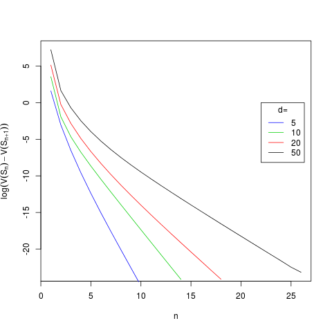
Figure 2: log-decrease of target function for iteration (19), different dimensions $d$

References

[1] Agueh, M. and Carlier, G. (2011). Barycenters in the Wasserstein space. SIAM J. Math Anal.
43, 904–924.
[2] Álvarez-Esteban, P.C., del Barrio, E. Cuesta-Albertos, J.A. and Matrán, C. (2011).
Uniqueness and approximate computation of optimal incomplete transportation plans. Ann. Institut Henri Poincaré
- P & S, 47, 358–375.
[3] Álvarez-Esteban, P.C., del Barrio, E. Cuesta-Albertos, J.A. and Matrán, C. (2015). Wide consensus for parallelized inference. Submitted.
[4] Ambrosio, L., Gigli, N. and Savaré, G. (2008). Gradient Flows in Metric Spaces and in the Space of Probability
Measures, 2nd ed. Birkhäuser.
[5] Benamou, J. D., Carlier, G., Cuturi, M., Nenna, L., and Peyre, G. (2015). Iterative Bregman projections
for regularized transportation problems. SIAM J. Sci. Comput., 37(2), 1111–1138.
[6] Bhatia, R. (1997). Matrix Analysis. Springer.
[7] Bishop, A. N., and Doucet, A. (2014). Distributed nonlinear consensus in the space of probability measures. arXiv Preprint arXiv:1404.0145.
[8] Brenier, Y. (1987) Polar decomposition and increasing rearrangement of vector
fields. C. R. Acad. Sci. Paris Ser. I Math., 305, 805–808.
[9] Brenier, Y. (1991). Polar factorization and monotone rearrangement of vector-
valued functions. Comm. Pure Appl. Math., 44, 375–417.
[10]
Carlier, G., Oberman, A., and Oudet, E. (2015). Numerical methods for matching for teams and Wasserstein barycenters. ESAIM Math. Model. Numer. Anal., to appear.
[11] Cuesta-Albertos, J. A. and Matrán, C. (1989). Notes on the Wasserstein metric in Hilbert spaces. Ann. Probab., 17, 1264–1276.
[12]
Cuesta-Albertos, J. A., Matrán, C., and Rodríguez-Rodríguez, J. (2003).
Approximation to probabilities through uniform laws on convex sets.
J. Theoretical Probab., 16, 363-376.
[13]Cuesta-Albertos, J. A., Matrán, C., and Tuero-Díaz, A. (1996). On lower bounds for the Wasserstein metric in a Hilbert space. J. Theoretical Probab., 9(2), 263–283.
[14]
Cuesta-Albertos, J. A., Matrán, C. and
Tuero-Díaz,, A. (1997). Optimal transportation plans and convergence in distribution. J. Multivariate Anal., 60, 72–83.
[15]
Cuesta-Albertos, J. A., Rüschendorf, L., and Tuero-Díaz, A. (1993). Optimal coupling of multivariate distributions and stochastic processes. J. Multivariate Anal., 46, 335–361.
[16]
Cuturi, M. and Doucet, A. (2013). Fast Computation of Wasserstein Barycenters, in Proceedings of the 31st International Conference on Machine Learning, 2014.
[17] Dudley, R. M. (1989). Real Analysis and Probability. Wadsworth & Brooks.
[18]
Evans, L.C. and Gariepy, R.F. (1992). Measure Theory and Fine Properties of Functions. Studies in Advanced Mathematics. CRC Press, Boca Raton,
FL.
[19]
Gelbrich, M. (1990). On a formula on the Wasserstein metric between measures on Euclidean and Hilbert spaces. Math. Nachr. 147, 185–203.
[20]
Le Gouic, T. and Loubes, J.M. (2015). Existence and consistency of Wasserstein barycenters. hal-01163262
[21]
Knott, M. and Smith, C. S. (1987). Note on the optimal transportation of distributions. J. Optimization Theory and Appl. 52, 323–329.
[22]
Knott, M. and Smith, C. S. (1994). On a generalization of cyclic-monotonicity
and distances among random vectors, Linear Algebra Appl.,199, 36–371.
[23]
McCann, R. J. (1995). Existence and uniqueness of monotone measure-preserving maps. Duke Mathematical Journal 80, 309–323.
[24] Niculescu, P. N. and Persson, L. E. (2006). Convex Functions and
their Applications: A Contemporary Approach. Springer.
[25] Rüschendorf, L. and Rachev, S. T. (1990). A characterization of random variables with minimum -distance. J. Multivariate Anal., 32, 48–54.
[26]
Rüschendorf, L., and Uckelmann, L. (2002). On the -coupling problem. J. Multivariate Anal., 81(2), 242–258. doi:10.1006/jmva.2001.2005
[27] Villani, C. (2003). Topics in Optimal Transportation. American Mathematical Society.
[28] Villani, C. (2008). Optimal transport: Old and New, Vol. 338. Springer Science &
Business Media.