Tunneling time in attosecond experiments, Keldysh, Mandelstam-Tamm and intrinsic-type of time.

Abstract

Tunneling time in attosecond and strong field experiments is one of the most controversial issues in today’s research, because of its importance to the theory of time, the time operator and the time-energy uncertainty relation in quantum mechanics. In O. Kullie (2015) we derived an estimation of the (real) tunneling time, which shows an excellent agreement with the time measured in attosecond experiments, our derivation is found by utilizing the time-energy uncertainty relation, and it represents a quantum clock. In this work, we show different aspects of the tunneling time in attosecond experiments, we discuss and compare the different views and approaches, which are used to calculate the tunneling time, i.e. Keldysh time (as a real or imaginary quantity), Mandelstam-Tamm time and our tunneling time relation(s). We draw some conclusion concerning the validity and the relation between the different types of the tunneling time with the hope, it will help to answer the the question put forward by Orlando et al G Orlando et al. (2014); *Orlando:2014II: tunneling time, what does it mean?. In respect to our result, the time in quantum mechanics can be, in more general fashion, classified in two types, intrinsic dynamically connected, and external dynamically not connected, to the system.

.1 Introduction

The area of time-energy uncertainty relation (TEUR) continues to attract the attention of many researchers until now, and it remains alive almost 90 years after its birth V. V. Dodonov and Dodonov (2015). It received, since 1980s, a ‘new breath’ due to the actual problems of quantum information theory and impressive progress of the experimental technique in quantum optics and atomic physics V. V. Dodonov and Dodonov (2015); A. Maquet et al. (2014). There is no doubt that the advent of ‘attophysics’ opens new perspectives in the study of time resolved phenomena in atomic and molecular physics A. Maquet et al. (2014). Since the appearance of the quantum mechanic the time was controversial, the famous example is the Bohr-Einstein weighing photon box Gedanken experiment. The crucial point is that, to date, there is no general time operator found, thus the uncertainty relation is used dependent upon the study case and usually reduced to the position-momentum uncertainty relation or used in a pragmatic way Mug (2008) (chap. 3). There is still common opinion that time plays a role essentially different from the role of the position in quantum mechanics (although it is not in line with special relativity), and that the time is not an operator but a parameter and hence does not obey an ordinary time-energy uncertainty relation (TEUR). Busch P. Busch (1990a, b) argued that the conundrum of the TEUR in quantum mechanics is related in first place to the fact that the time is identified as a parameter in Schrödinger equation (SEQ). Hilgevoord J. Hilgevoord (2002) has showed that there is nothing in the formalism of the quantum mechanics that forces us to treat time and position differently. Observables such as position, velocity, etc. both in classical mechanics as well as in quantum mechanics, are relative observables, and one never measures the absolute position of a particle, but the distance in between the particle and some other object J. Hilgevoord (2002); Y. Aharonov and Reznik (2000). Hilgevoord concluded J. Hilgevoord (2002) that when looking to a time operator a distinction must be made between universal time coordinate $t$, a c-number like a space coordinate, and the dynamical time variable of a physical system suited in space-time, i.e. clocks.

Indeed there have been many attempts to construct time as an operator M. Razavy (1967); T. Goto et al. (1981); D. Han et al. (1983); Z.-Y. Wang and Xiong (2007), Busch P. Busch (1990a, b) classified three types of time in quantum mechanics: external time (parametric or laboratory time), intrinsic or dynamical time and observable time. External time measurements are carried out with clocks that are not dynamically connected with the object studied in the experiment, and usually called parametric time. The intrinsic-type of time is measured in terms of the physical system undergoing a dynamical change, the time is defined through the dynamical behavior of the quantum object itself, where every dynamical variable marks the passage of time. The third type, according to Busch, is the observable time or event time, for example the time of arrival of the decay products at a detector. One of the most impressive debates about the time and the TEUR in quantum mechanic is the (Bohr-)Einstein weighing L. F. Cooke (1980); Y. Aharonov and Reznik (2000), or short, Bohr-Einstein Gedanken experiment (Bohr-Einstein-GE). A photon is allowed to escape from a box through a hole, which is closed and opened temporarily by a shutter, the period of time is determined by a clock, which is part of the box system, which means that the time is intrinsic and dynamically connected with the system under consideration. The total mass of the box before and after a photon passes is measured. Bohr showed that the process of weighing introduces a quantum uncertainty (in the gravitational field) which leads to an uncertainty in time $\tau$, the time needed to pass out of the box that usually called passage time P. Busch (1990a, b), in accordance with the TEUR:

$${\,\,\Delta T\cdot\Delta E\geq\frac{\hbar}{2}}$$ (1)

Aharonov and Rezinik Y. Aharonov and Reznik (2000) offer a similar interpretation, that the weighing leads, due to the back reaction of the system underlying a perturbation (energy measurement), to an uncertainty in the time of the internal clock relative to the external time Y. Aharonov and Reznik (2000). Hence for quantum systems it is decisive to observe the time from within the system or using an internal clock.

.2 Basic concepts of the attosecond experiment

In attosecond experiment the idea is to control the electronic motion by laser fields that are comparable in strength to the electric field in the atom. In today’s experiment usual intensities are $\sim 10^{14}\,Wcm^{-2}$, for more details we refer to the tutorial F. Krausz and Ivanov (2009); J. M. Dahlström et al. (2012). In the majority of phenomena in attosecond physics, one can separate the dynamics into a domain ”inside” the atom, where atomic forces dominate, and “outside“, where the laser force dominates, a two-step semi-classical model, pioneered by Corkum P. B. Corkum (1993). Ionization as the transition from ”inside” to ”outside” the atom plays a key role for attosecond phenomena. A key quantity here is the Keldysh parameter $\gamma_{{}_{K}}=\frac{\sqrt{2I_{p}}}{F}\omega$, where $I_{p}$ denotes the ionization potential of the system (atom or molecule)

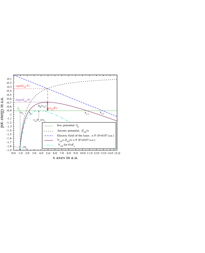
Figure 1: Graphic display of the potential curves, the barrier width and the two inner and outer points $x_{e,\pm}={(I_{p}\pm\delta_{z})/2F}$, the ”classical exit“ point $x_{e,c}=I_{p}/F$ and the $x_{m}(F)=\sqrt{Z_{{}_{eff}/F}}$ the position at maximum of the barrier height, (note $x_{a}=x_{m}(F=F_{a})$) see text.

$\omega$ is the laser circular frequency and $F$ is the peak electric field strength at maximum. Here and below we use atomic units where $\hbar=m=e=1$, the Planck constant, the electron mass and the unit charge are all set to 1. At values $\gamma_{{}_{K}}>1$ one expects predominantly photo-ionization, while at $\gamma_{{}_{K}}<1$ ionization happens by the tunneling process, which means that the electron does not have enough energy to ionize but tunnels through a barrier made by the Coulomb potential and the electric field of the laser pulse to escape at the exit point to the continuum, as shown in fig 1.

The tunneling time (T-time) in attosecond experiment is usually thought, in a simplified picture, as the time spent to pass the barrier region, i.e. the classically forbidden region, and escape at the exit point of the barrier (denoted $\tau_{{}_{T,d}}$) O. Kullie (2015), and the (quantum) particle (an electron) undergoing this process spends a time that is, the time needed from the moment of entering the barrier region to the moment of escaping the barrier region, in the tunneling direction. This picture, despite its simplicity, is common between theory and experiment O. Kullie (2015), see sec .5. Moreover, in O. Kullie (2015) we have defined a time-interval needed to reach the entrance of the barrier (denoted $\tau_{{}_{T,i}}$), after it is shaken off by the laser field at its initial position $x_{i}$. $\tau_{{}_{T,d}}$ is also similar to the traversal time used in context of the tunneling approaches E. H. Huge and Støvneng (1989); Landauer and Martin (1994) such as the Feynman path integral (FPI) approach N. Yamada (2004); D. Sokolovski et al. (1994, 1990); A. S. Landsman and Keller (2015) (and Mug (2008) chap. 7). But in contrast to FPI, we do not make any assumption about paths inside the barrier, where as well-known, the FPI approach is based on all paths starting at the entrance of the barrier at $t=0$ and end at the exit of the barrier at time $t=\tau$, which defines a time duration $\tau$. A second type of T-time we invented is what we call the symmetrical T-time or the total T-time (denoted $\tau_{{}_{T,sym}}=\tau_{{}_{T,i}}+\tau_{{}_{T,d}}$), where we found that it can be easily calculated from the symmetry property of the T-time. $\tau_{{}_{T,sym}}$ is the time accounted from the moment of starting the interaction process, where the electron gets a shake-off, responds and jumps up to the tunneling “entrance“ point taking the (opposite) orientation of the field, then pass the barrier region to the ”exit” point and escapes the barrier to the continuum.

.3 Theory and model

Our start is a model of Augst et al. S. Augst et al. (1989, 1991), where the appearance (or threshold) intensity of a laser pulse for the ionization of the noble gases is predicted. The appearance intensity is defined S. Augst et al. (1989) as the intensity at which a small number of ions is produced. In this model (in atomic units) the effective potential of the atom-laser system is given by

$$V_{eff}(x)=V(x)-xF=-\frac{Z_{eff}}{x}-xF,$$ (2)

where $F=F_{m}$ is the field strength at maximum of the laser pulse (in this work in all our formulas $F$ stands for $F_{m}$), and $Z_{eff}$ is the effective nuclear charge that can be found by treating the (active) electron orbital as hydrogen-like, similar to the well-known single-active-electron (SAE) model H. G. Muller (1999); X. M. Tong and Lin (2005). The choice of $Z_{eff}$ is easily recognized for many-electron systems and well-known in atomic, molecular and plasma physics S. Augst et al. (1991); Schlüter (1987); R. Lange and Schlüter (1992); I. Dreissigacker and Lein (2013). We take a one-dimensional model along the x-axis as justified by Klaiber and Yakaboylu et al M. Klaiber et al. (2013); E. Yakaboylu et al. (2013). Indeed the barrier height at a position $x$ is, compare fig 1:

$$\overline{h_{B}(x)}=\mid h_{B}(x)\mid=\mid E-V_{{}_{eff}}(x)\mid=\mid-I_{p}+\frac{Z_{eff}}{x}+xF\mid$$ (3)

that is equal to the difference between the ionization potential and effective potential $V_{eff}(x)$ of the system (atom+laser) at the position $x$, where $E=-I_{p}$ is the binding energy of the electron before interacting with the laser. The crossing points $x_{e,\pm}$ of $V_{{}_{eff}}(x)$ with the $-I_{p}$-line are given by $h_{B}(x)=0$

$$x_{e,\pm}=\frac{I_{p}\pm\delta_{z}}{2F}\Rightarrow d_{B}=x_{e,+}-x_{e,-}=\frac{\delta_{z}}{F},$$ (4)

$$x_{e,c}=x_{e,+}+x_{e,-}=\frac{I_{p}}{F}=d_{c}$$

where $d_{B}$ is the barrier width and $x_{e,c}$ is usually called the “classical exit” point, it is the intersection of the field line $-xF$ with $I_{p}$-line, which equals what is usually called the “classical” barrier width $d_{c}$. $\delta_{z}=\delta_{z}(F)$ is given in eq (6), we emphasize the dependence of $\delta_{z}$ on $Z_{eff}$ as done by S. Augst et al. (1991); I. Dreissigacker and Lein (2013). Augst et al S. Augst et al. (1989) calculated the position of the barrier maximum $x_{m}$, from $\partial{V_{eff}(x)}/\partial{x}=0$ (compare fig 1, the lower green curve) and obtained an expression for the atomic field strength $F_{a}$,

$$-\frac{Z_{eff}}{x_{a}}-x_{a}F=-I_{p}\Rightarrow F_{a}=\frac{I_{p}^{2}}{4Z_{eff}}$$ (5)

and the appearance intensity $I_{a}=F^{2}_{a}$.

Indeed, we can get $x_{m}$ and the maximum $h_{B}(x_{m})$ from the derivative of eq (3), ${\partial h_{B}(x)}/{\partial x}=0$. The maximum of the barrier height $h_{B}(x_{m})$ for arbitrary field strength lies at $\,x_{m}(F)=\sqrt{Z_{eff}/F}$ O. Kullie (2015). Fortunately, eq (5) can be generalized as the following, for a field strength $F\leq F_{a}$:

$$F\leq\frac{I_{p}^{2}}{4Z_{eff}}\Rightarrow\delta_{z}^{2}=I_{p}^{2}-4Z_{eff}F\geq 0$$ (6)

The equality $\delta_{z}=0$ is valid for $F=F_{a}$. Indeed, $\delta_{z}=\delta_{z}(F)=\sqrt{I_{p}^{2}-4Z_{eff}F}$ is a key quantity, it controls the tunneling process, and determines the time ”delay” under the barrier $\tau_{{}_{T,d}}$ and the total or the symmetrical T-time $\tau_{{}_{T,sym}}$, as we will see in sec. .4. The maximum barrier height $h_{B}(x_{m})$, see fig 1, is

$$h_{B}(x_{m})=\mid\!-I_{p}-V_{eff}(x_{m})\!\mid=\mid\!-I_{p}+\sqrt{4Z_{eff}F}\!\mid$$ (7)

by setting $h_{B}(x_{m})=0$ one obtains $F_{a}=I_{p}^{2}/(4Z_{eff})$, which is equivalent to setting $V_{eff}(x_{m})=-Ip$ as done by Augst et el S. Augst et al. (1989, 1991), and can be easily verified from eqs (3), (5).

.4 Tunneling time

In O. Kullie (2015) we showed that the uncertainty in the energy can be quantitatively discerned from the atomic potential energy at the exit point $\Delta E\sim\mid\!V(x_{e})\!\mid=\mid\!-\frac{Z_{eff}}{x_{e}}\!\mid$ for arbitrary subatomic field strength $F\leq F_{a}$. Then we drew the attention to the particular importance of the symmetry property of time, for example Aharonov-Bohm defined a time operator Y. Aharonov and Bohm (1961); H. Paul ; G. R. Allcock (1969a) for a free particle. $\hat{T}=\frac{1}{2}(\hat{x}\,\hat{p}^{-1}+\hat{p}^{-1}\hat{x})$, whereas Olkhovsky and Recami presented V. S. Olkhovsky (2014); *Olkhovsky:2009; *Olkhovsky:2004; *Olkhovsky:1970 a more elaborate treatment (the so-called bilinear form), see also Allcock G. R. Allcock (1969a). Such operators (given by Aharonov-Bohm or Olkhovsky) have the property of being maximally symmetric in the case of the continuous energy spectra, and the property of quasi-self-adjoint operators in the case of the discrete energy spectra V. S. Olkhovsky (2009), and are the closest best thing to a self-adjoined operator and satisfy the conjugate relation with the Hamiltonian and therefore implies an ordinary TEUR V. S. Olkhovsky (2009) and Mug (2008) (chap. 1). We used this property in the tunneling process, and we obtained what we called the symmetrical T-time given by O. Kullie (2015):

$$\tau_{{}_{T},sym} = \tau_{{}_{T,+}}+\tau_{{}_{T,-}}=\tau_{{}_{T,i}}+\tau_{{}_{T,d}}$$

$$= \frac{1}{2}\left(\frac{1}{\Delta E^{-}}+\frac{1}{\Delta E^{+}}\right)$$

$$= \frac{1}{2}\left(\frac{1}{(Ip+\delta_{z})}+\frac{1}{(Ip-\delta_{z})}\right)=\frac{I_{p}}{4Z_{eff}F}$$

where we defined $\tau_{{}_{T,\pm}}=1/(2\Delta E^{\mp})={(2(Ip\pm\delta_{z}))}^{-1}$, or $(1/2)\Delta E^{\pm}=\Delta E(x_{e,{\pm}})=\mid\!\!-\frac{Z_{eff}}{x_{e,\pm}}\!\!\mid$, and $\tau_{{}_{T,i}}=\tau_{{}_{T,+}}$, $\tau_{{}_{T,d}}=\tau_{{}_{T,-}}$. The barrier itself causes a delaying time relative to the atomic field strength given by:

$$\tau_{{}_{T,d}}\equiv\frac{1}{2\Delta E^{+}}=\frac{1}{2\,(I_{p}-\delta_{z})}=\tau_{{}_{T,-}}\,(\mbox{for }F\leq F_{a})$$ (9)

which we call $\tau_{{}_{T,d}}$ meaning that is the time delay with respect to the atomic field strength (the time duration) to pass the barrier region (in the direction $x_{{{}_{e},-}}\!\rightarrow\!x_{{}_{e,+}}$) and escape at the exit point $x_{e,+}$ to the continuum, for more details see O. Kullie (2015). The first term in eq (.4) is the time needed to reach the ”entrance“ point $x_{e,-}$, compare fig 1.

$$\tau_{T,i}=\tau_{(x_{i},x_{e,-})}=\frac{1}{2\Delta E^{-}}=\frac{1}{2(I_{p}+\delta_{z})}=\tau_{{}_{T,+}}$$ (10)

At the limit $F\rightarrow F_{a}$, $\delta_{z}\rightarrow 0$, and the tunneling time becomes the ionization time,

$$\tau_{{}_{T},sym}=\frac{1}{2Ip}+\frac{1}{2Ip}=\frac{1}{Ip}$$ (11)

accordingly, the tunneling happens in two steps O. Kullie (2015), the shake-up $\tau_{{}_{T},i}=\frac{1}{2Ip}$ and shake-off $\tau_{{}_{T},d}=\frac{1}{2Ip}$. For $F=F_{a}$ the two steps happen with equal time duration and are not strictly separated, unlike the case for subatomic field strength $F<F_{a}$ due to the barrier, as discussed in O. Kullie (2015). It is nice to see that the mean of the uncertainties $\Delta E_{M}=\frac{1}{2}\left({\Delta E^{-}}+{\Delta E^{+}}\right)=I_{p}$, this has led some authors to mention that a T-time of the order $1/I_{p}$ can be estimated via TEUR, when assuming an energy uncertainty of order of $Ip$ M. Klaiber et al. (2013).

The T-time found in eq (.4) can also be derived in an elegant way, when we assume that the barrier height eq (7) corresponds to a maximally symmetric operator as the following. The barrier height eq (7) $h_{B}(x_{m})\equiv h_{M}$ can be related to a (real) operator $\widehat{h}_{B}(x_{m})$

$$\widehat{h}_{M}^{\pm}=-I_{p}\pm\sqrt{4Z_{eff}F}=-I_{p}\pm\Delta$$ (12)

and the uncertainty in the energy caused by the barrier

$$\left(\widehat{h}_{M}^{-}\widehat{h}_{M}^{+}\right)^{1/2}=[(-I_{p}-\Delta)(-I_{p}+\Delta)]^{1/2}=\delta_{z}$$ (13)

From this we get ${\Delta E^{\pm}}=abs(-Ip\pm\delta_{z})$ and hence $\tau_{{}_{T,d}}$, $\tau_{{}_{T,i}}$ and $\tau_{{}_{T,sym}}$ by the virtue of eq (1), where we assumed that the time is intrinsic and has to be considered with respect to the atomic field strength, i.e. to the ionization potential $I_{p}$, see discussion in subsec .6.2.

.5 Comparison to the experiment

In fig 2 we show the results for $\tau_{{}_{T,d}}$ eq (9), and the symmetrical (or total) T-time $\tau_{{}_{T,sym}}$ of eq (.4). Note eq (9), is the second term of eq (.4), which is the actual T-time, i.e. the time needed to pass the barrier region $(x_{e,-}\rightarrow x_{e,+})$ and escape at the exit point to the continuum. The plotted result is for the He-atom together with the experimental result of P. Eckle et al. (2008a); *Eckle:2008. The experimental data and the error bars in the figure were kindly sent by A. S. Landsman A. S. Landsman et al. (2014). We plotted the relations at the values of the field strength at the maximum of the elliptically polarized laser pulse ($\lambda=735$, elliptical parameter $\varepsilon=0.87$, $F=F_{0}/\sqrt{1+\varepsilon^{2}}$) used by the experiment exactly as given in A. S. Landsman et al. (2014). Concerning the experiment by the group of Keller et al A. S. Landsman et al. (2014), the time delay due the barrier is measured indirectly $t_{T}^{exp}=\frac{(\theta_{m}-\theta_{C})}{\omega}$, where $\omega$ is the laser frequency, $\theta_{m}$ the angular offset of the center of angular distribution, and $\theta_{C}$ a correction due to the Coulomb force of the ion calculated by classical trajectory simulation P. Eckle et al. (2008a, b); A. S. Landsman et al. (2014); A. S. Landsman and Keller (2015); C. Hofmann et al. (2013). Unfortunately, in this experiment the beginning of the interaction between the laser field and the bound electron cannot be directly observed or exactly determined. The time zero $t_{0}^{exp}$ is one of the assumption of the model, which used to interpret the data. Consequently, in the experiment it is not possible to distinguish between the instant of the interaction $t_{0}=0$ and the instant when the electron enters the barrier region, say $t_{T,l}$, C. Hofmann and Cirelli . However, arguing that the probability of tunneling is highest when the barrier is shortest, corresponding to $t_{0}^{exp}$ C. Hofmann and Cirelli , suggests that the data from the measurement are comparable to the time delay caused by the barrier (the time spent in the classical forbidden region C. Hofmann and Cirelli ), which means that $t_{T}^{exp}$ corresponds or (approximately) equals the actual T-time delay of our model $t_{T}^{exp}\approx\tau_{T,d}$.

The two different effective charge models are from Kullie O. Kullie , with $Z_{{}_{eff,K}}=1.375$ and Clementi E. Clementi and Raimondi (1963) with $Z_{{}_{eff,C}}=1.6875$. For the $\tau_{{}_{T,d}}$ we see an excellent agreement with the experiment. $\tau_{{}_{T,d}}$ corresponds to the T-time measured in the experiment, that is the time (interval) needed to pass the barrier region from the entrance to the exit point and escape to the continuum with a shake-off O. Kullie (2015), or between the instant of orientation at $x_{e,-}$ and the instant of ionization at $x_{e,+}$, which is the time spent in the classically forbidden region P. Eckle et al. (2008a).

In fig 2 we see that the difference between the total or symmetrical T-time $\tau_{{}_{T,sym}}$ and the (actual) T-time $\tau_{{}_{T,d}}$ is small, because the second term $\tau_{{}_{T,d}}$ in eq (.4) incorporates the delay time caused by the barrier, and is the main time contribution to the tunneling process for a large barrier. Whereas the first part term $\tau_{{}_{T,i}}$, is due to the shake-up of the electron by the field moving it to the ”entrance” $x_{e,-}$, which is small for a small $F$. For a large field strength the two parts become closer because the barrier width is getting smaller $\delta_{z}/F=(x_{e,+}-x_{e,-})\rightarrow 0$ and for the appearance intensity ($\delta_{z}=0)$ they are equal.

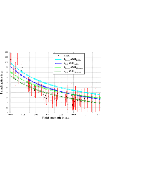
Figure 2: T-time $\tau_{{}_{T,d}}$ eq (9) and $\tau_{{}_{T,sym}}$ eq (.4), for two different $Z_{eff}$ models. Time is in attosecond units vs laser field strength in atomic units, corresponds to the tunneling ionization of the He-Atom in strong field, in good agreement with experimental result A. S. Landsman and Keller (2014); A. S. Landsman et al. (2014); P. Eckle et al. (2008a, b). Experimental values are kindly sent by A. S. Landsman A. S. Landsman et al. (2014).

For small $F\lesssim 0.055\,au$, $Z_{eff,K}$ gives a better agreement with the experiment, whereas for larger field strength $Z_{eff,C}$ is more reliable, where multielectron effects are expected due to the decreasing width of the barrier and the tunneling electron is closer to the first one, when it traverses the barrier.

At the limit $F=F_{a}$ of the sub-atomic field strength $F<F_{a}$, the tunneling process is out and an ionization process called ”above the barrier decay“ is beginning. For super-atomic field strength $F>F_{a}$, $\delta_{z}$ becomes imaginary (and so the crossing points, compare eq (4)), which indicates that the real part $\frac{1}{2I_{p}}$ of $\tau_{{}_{T,d}}$ or $\tau_{{}_{T,i}}$, is the limit for a ”real” (see below) time (tunnel-)ionization process. Indeed, in this case the atomic potential is heavily disturbed and the imaginary part of the time $\tau_{{}_{T,d}}$ is obviously, due to the ionization or the release of the electron (to the continuum) from a lower level than $-Ip$ (and possibly escaping with a high velocity), where the ionization happens mainly by a shake-off step N. B. Delone and Krainov (2000) (chap. 9). Here we see the clear difference between the quantum mechanical and the classical clocks Y. Aharonov and Bohm (1961). Classically we can make the interaction time with the system arbitrarily small, the real part of the time can be made arbitrary small, and an imaginary part is absent. In quantum mechanics the tunneling-ionization time has a real part limit $\tau_{{}_{T,d}}=1/(2I_{p})$, an imaginary part arises when the field strength is larger than the atomic field strength $F_{a}$, in both terms $\tau_{{}_{T,i}}$ and $\tau_{{}_{T,d}}$.

However, in our treatment, although, $\tau_{{}_{T,i}},\tau_{{}_{T,d}}$ have an imaginary part for $F\geq F_{a}$, the total or symmetrical T-time remains real

$$\tau_{{{}_{T},sym}}=\frac{I_{p}}{4Z_{eff}F}=\frac{1}{I_{p}\xi}=\frac{1}{I_{p}}(\frac{F_{a}}{F})$$

for ionization processes with an arbitrary field strength, where $\xi=\frac{F}{F_{a}}$ is the perturbation parameter, for which the perturbation theory is valid, when $\xi\ll 1$. $\tau_{{}_{T,sym}}$ is small for $\xi=\frac{F}{F_{a}}\rightarrow c,c\geq 1$, and probably the above relation ($\tau_{{}_{T,sym}}$) loses its validity for $F>F_{a}$, suspecting a break of some symmetry at $F=F_{a}$, non-linear effects arise and the interaction becomes physically a different character. It is apparent from $\tau_{{{}_{T},sym}}$ eq (.4), that the T-time has no imaginary part, when the symmetry of the time is considered, i.e. assuming the maximally symmetric (quasi-self-adjoint) property discussed in detail by Olkhovsky V. S. Olkhovsky (2009).

.6 Tunneling, Mandelstam-Tamm and Keldysh time

.6.1 Preliminary discussion

An important point in our treatment (T-time approach) is that, our T-time is intrinsic or dynamically connected to the system and is the T-time of a quantum particle, whereas for example the Keldysh time (K-time) $\tau_{K}$ is defined for a classical particle, and $\tau_{K}\!\!=\!\!{\sqrt{2I_{p}}}/{F}$ is determined as G Orlando et al. (2014); *Orlando:2014II

$$\overline{\tau}_{K}\!\!=\!\!d_{c}/|v|$$ (14)

where $d_{c}\!\!=\!\!I_{p}/F$ is the “classical” barrier width (compare with $d_{B}$ eq (4)) and $|v|$ is the average speed of an electron under the static barrier. We note that in this definition $d_{c}$ is equal to the ”classical“ exit point $x_{e,c}$ eq (4), compare fig 1. It is easy to find that the average speed $|v|$ is the (arithmetic) mean of the speed $\overline{v}=(v_{e}+v_{0})/2\!=\!{(0+v_{0})}/2\!=\!\sqrt{2I_{p}}/2$, neglecting the atomic potential, where $v_{e}=0$ is the velocity at the exit point according to the strong field approximation (SFA). $\overline{v}$ equals the ”Wirkungswellen-” velocity (action-wave velocity) $u$ of a classical particle with a total energy equal to the kinetic energy $E=T,V=0$, $u=\frac{|E|}{\sqrt{2T}}\!=\frac{\!\sqrt{2I_{p}}}{2}$ Nolting (1990) (chap 3.6, p. 196). Then, $\tau_{K}=d/\overline{v}=(I_{p}/F)\cdot(2/\sqrt{2I_{p}})=\sqrt{2I_{p}}/F$ and the electron tunnels like a classical particle with $\overline{v}=u$ through the barrier (neglecting the potential $V=0$). Hence our T-time $\tau_{T,d}$ (and $\tau_{T,\pm},\tau_{T,sym}$) represents a quantum clock, whereas $\tau_{K}=\overline{\tau}_{K}$ represents a laboratory or external time, it cannot describe the attosecond experiment and contradicts the TEUR as mentioned by Rzazewski K. Rzazewski and Roso-Franco (1993).

Orlando et al G Orlando et al. (2014); *Orlando:2014II calculated the Mandelstam-Tamm time (MT-time, $\tau_{MT}$) and the result equals the K-time $\tau_{MT}\!\!=\!\!\tau_{K}=\overline{\tau}_{K}$. They assumed that the uncertainty in the energy due to the barrier is given by the standard deviation $\delta E\!\!=\!\!\Delta H\!\!=\!\!\sqrt{<H^{2}>-<H>^{2}}$, where $H=H_{0}-xF$ and $H_{0}$ is the Hamiltonian of the unperturbed atomic system (and $(\delta p)^{2}\sim 2<\!\!T\!\!>=2I_{p}$) G Orlando et al. (2014); *Orlando:2014II. First, it is known that the standard deviation can be a very unreasonable measure for the uncertainty in the energy J. Uffink (1993) especially for wave functions with long tails. Secondly, $\Delta H$ will not lead to a correct T-time, because the uncertainty in the energy is not determined by $\Delta H$ but by the barrier height given by eqs (7), (12-13), which, at the end, leads to $\Delta E^{\pm}$ and the correct T-time $\tau_{{}_{T,\pm}}$. Note in our case the height and the width of the barrier are not independent, both depend on the filed strength, see eqs (7), (4) . However, it is somehow puzzling to see that our $\delta E=abs(-I_{p}+\delta_{z})=(Ip-\delta_{z})=\Delta E^{+}$ is the expectation value of the Hamiltonian $H_{B}=H_{0}+(x_{e,+}-x_{e,-})F=(-Ip+\delta_{z})$, where $d_{B}=(x_{e,+}-x_{e,-})=\delta_{z}/F\neq d_{c}$ is the barrier width (compare eq (4)), this leads to the correct T-time eq (9) by the virtue of eq (1). From this, it is also true that the time should be considered from within the system (internal time), where the reference point is (the ionization potential) $abs(E_{0})=I_{p}$, which is overcome when $F=F_{a}$, and the system undergoes an (ejection of an electron or a threshold) ionization process (no barrier). The delay time is found relative to the reference point from the perturbation $d_{B}\cdot F=(\frac{\delta_{z}}{F})F=\delta_{z}$ as we already discussed, which becomes zero at atomic field strength, $\delta_{z}(F_{a})=0$ (no barrier), and the T-time $\tau_{T,d}$ is reduced to $1/(2I_{p})$, the second part of the total ionization time, see eq (11).

A further point, Orlando et al G Orlando et al. (2014); *Orlando:2014II obtained a similar result by numerical investigation of the wave packet dynamics with the same Hamiltonian $H$, which in turn, makes the puzzle more difficult to understand. Nevertheless, most important is the preparation of the system and its Hamiltonian and how to observe the time in the system, see discussion further in subsec .6.2 and subsec .6.4. In fact Maquet et al A. Maquet et al. (2014) noted that a time-delay requires to choose a reference system, delays in numerical simulation can refer in principle to any arbitrarily chosen reference A. Maquet et al. (2014), see next subsec .6.2.

.6.2 Internal- and external- time frame

Indeed, we can follow the procedure of Orlando et al but with two crucial differences. The first difference is, we take $<x^{2}>=d_{B}^{2}$, which means that the particle is de-localized over the whole barrier instead of $1/(\Delta p)^{2},\,(\Delta p)^{2}=2<\!\!T\!\!>$ used by Orlando et al G Orlando et al. (2014); *Orlando:2014II, this assumption is quantum-mechanically valid. Calculating now the ”variance” as done in G Orlando et al. (2014); *Orlando:2014II, we get $\delta E\!\!=\left((I_{p}^{2}-d_{b}^{2}\cdot F^{2})-I_{p}^{2}\right)^{1/2}=\delta_{z}$. The second difference, we have to take our uncertainty in the energy (and thus the T-time) relative to the binding energy in the ground state $-Ip$, which is decisive (see below and compare fig 1), thus we obtain $(-Ip+\delta)$ (or $(-Ip\pm\delta)$ considering the symmetry), this leads to the ”correct” T-time $\tau_{T,d}$ (or $\tau_{T,\pm}=(-Ip\mp\delta)^{-1}$ and $\tau_{T,sym}$).

In fact, one can argue that $-Ip$ must be taken to avoid the divergence of the time to infinity for $F=F_{a}$, because it is physically incorrect, as $\delta_{z}(F_{a})=0$, which in turn can be seen as an initialization of the internal clock, i.e. the T-time is counted as a delay with respect to the ionization at $F_{a}$ (the limit of the subatomic field strength). This is exactly what Maquet et al A. Maquet et al. (2014) alluded to, quoting them “the definition of a ‘time-delay’ requires to choose a ‘reference’ system.” The other limit, i.e. for $F\rightarrow 0,\,(I_{p}-\delta)\rightarrow 0$ is then the multiphoton regime, the tunneling did not take place and for $F=0,\delta_{z}=I_{p}\Rightarrow\tau_{T,d}=\infty$, hence nothing happens. That is exactly the well-known limit of an energy eigenstate of the MT-time relation, where the rate of change of a property decreases with increasing sharpness of the prepared energy $(-I_{p}+\delta_{z}(F\rightarrow 0))\rightarrow 0$.

Furthermore, we can consider the barrier width as the sum of the distances to reach, and from the ionization exit $x_{a}$ (at the atomic field strength), then (compare fig 1)

$$d_{B}=\delta_{z}/F=x_{e,+}-x_{e,-}=(x_{a}-x_{e,-})+(x_{e,+}-x_{a})$$

which causes an energy “uncertainty“ equal to $abs(-I_{p}+\delta_{z})=abs(-I_{p}+(\delta_{z}/F)F)=abs(-I_{p}+d_{B}F)$. It can be considered as the distance to the ionization limit ($d_{B}=0,\delta_{z}=0$) on the energy scale, and hence the time delaying $\tau_{T,d}$ to pass the barrier region. The point is, one would say that the two points $x_{e,\pm}$ are similar to the two slits (in the double slit experiment) with a distance $d_{B}$ (between the slits).

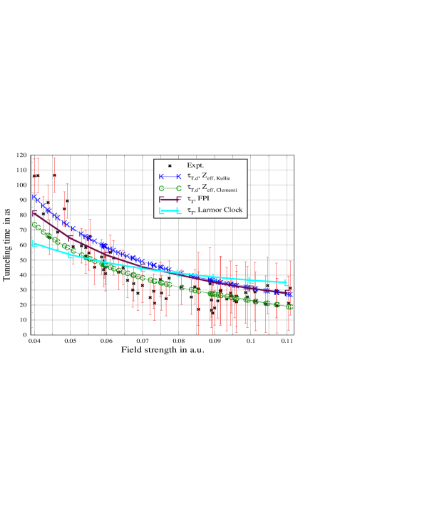
Figure 3: T-time $\tau_{{}_{T,d}}$ eq (9) for two different $Z_{eff}$ models as in fig 2 together with the FPI and Larmer Clock results A. S. Landsman et al. (2014), and the experimental result P. Eckle et al. (2008a, b); A. S. Landsman et al. (2014). Experimental values, the FPI and Larmer result are kindly sent by A. S. Landsman and C. Hofmann A. S. Landsman et al. (2014); C. Hofmann et al. (2013).

Accordingly, in the Feynman path integral formalism, the dwell time or the residence time (which is the time a particle spends in the barrier region), can be seen as a result of the interference between the wave packets or paths. Forwards (to $x_{e,+}$) and backwards (to $x_{e,-}$) tunneling correspond to the transmission and reflection amplitudes of the wave packet, respectively. This picture strengthens the good agreement between our result and FPI shown fig 3.

For the experimental setup the internal time view is not a crucial point, since in the experiment one extracts the internal information of the system from the output on the screen, whereas from a theoretical point of view it is very crucial, and a controversial discussion about the T-time is continuing. As already mentioned above Maquet et al pointed out that the definition of a ‘time-delay’ requires to choose a ‘reference’ system. Delays in ‘Gedanken’ experiments or in numerical simulations can refer in principle to any arbitrarily chosen reference A. Maquet et al. (2014). The situation is similar to what occurs in the special relativity, where a moving particle has its own time in its inertial frame, which differs from the time of the viewpoint of another inertial frame. A well-known example in this context, is the Muon decay, which can be found in introductory books. About $10000$ Muons reach every square meter of the Earth’s surface per minute. Although their lifetime without relativistic effects would allow a half-survival distance of only about $456m$ at most (as seen from Earth). The time dilation effect of special relativity (from the viewpoint of the Earth) allows cosmic ray secondary Muons to survive the flight to the Earth’s surface, since in the Earth frame, the Muons have a longer half lifetime due to their high velocity $0,9997\,c$, where $c$ is the speed of light. From the viewpoint (inertial frame) of the Muon, on the other hand, it is the length contraction effect of special relativity which allows this penetration, since in the Muon frame, its lifetime is unaffected, but the length contraction causes distances through the atmosphere and Earth to be far shorter than these distances in the Earth rest-frame. In our case of the T-time, it is not the relativistic effect, but observing the time from within the system (internal clock Y. Aharonov and Reznik (2000)), which differentiates it form the classical view. And although the relativistic effects in this case are negligible, the special relativity point of view is helpful, first to understand our current case and second, it could be necessarily (by using Dirac instead of SEQ) to establish the comparability of space and time on equal footing, where the symmetry of the time is then naturally embedded in the theory M. Bauer (2014, 1983); I. E. Antoniou and Misra (1992); E. Prugovec̆ki (1982). However, Dodonov V. V. Dodonov and Dodonov (2015) claims that no unambiguous and generally accepted results have been obtained so far.

.6.3 Critique of the Keldysh time and beyond

We discuss here some points about the K-time and MT-time, with the hope, that they are hints in understanding the puzzle of the T-time in attosecond experiment and the different views to calculate it.

First, one of the failures of K-time comes form its inadequate definition. Then, the difference between $d_{c}$ and $d_{B}$ is large (compare eq (4) and fig 1) $d_{B}<d_{c},d_{c}-d_{B}=(I_{p}-\delta_{z})/F=2x_{e,-}$, and although

$$\lim_{F\to 0}d_{B}=\lim_{F\to 0}\frac{\delta_{z}}{F}=\lim_{\xi\to 0}\frac{I_{p}}{F}\sqrt{1-\xi}=\frac{I_{p}}{F}=d_{c}$$

but for $F\rightarrow 0,(\xi=\frac{F}{F_{a}}\ll 1,\mbox{the perturbation regime})$, for a fixed frequency $\omega$, one obtains $\gamma_{K}(F\rightarrow 0)=\omega\cdot\tau_{K}(F\rightarrow 0)\,\gg\,1$ and that is the region of photo-absorption N. B. Delone and Krainov (2000) and tunneling is less probable compared with the multiphoton processing, because the K-time is based on the competition with the absorption of quanta K. Rzazewski and Roso-Franco (1993). Thus the tunneling is unlikely to happen at a (real) time interval length equal to K-time for small $F$. Moreover, for stronger field ($F\rightarrow F_{a}$) $\delta_{z}$ is small, hence $d_{B}(F\rightarrow F_{a})\approx 0$ is much smaller than $d_{c}$ $(\lim_{\xi\to 1}\frac{d_{B}}{d_{c}}=\lim_{\xi\to 1}\sqrt{1-\xi}=0)$. For $F=F_{a},d_{B}=0$, whereas $d_{c}=I_{p}/F_{a}=\frac{I_{p}}{Ip^{2}/4Z_{eff}}=4Z_{eff}/I_{p}$. Which means that the definition of the “classical“ barrier width as usually done to calculate the K-time, is inaccurate and inadequate.

And second, it is interesting to show that the MT-time $\tau_{MT}$ can be directly obtained. Then, $\tau_{MT}$ can be obtained by using the momentum $\hat{p}$ of the tunneling-electron as a dynamical observable, $\tau_{MT}$ results from its definition (again neglecting the atomic potential), using $(\Delta p)^{2}=2<T>$ as done by Orlando et al G Orlando et al. (2014); *Orlando:2014II we get:

$$\tau_{MT}^{p}=\frac{\Delta p}{\mid\frac{d}{dt}<p>\mid}=\frac{\sqrt{2I_{p}}}{F}=\tau_{MT}$$ (15)

In fact, this is the classical definition of the time a particle spends, when it moves rectilinear with a deceleration $F$ and an initial/final momentum $p_{0}/p_{f}$ between the initial and final moment $t_{0},t_{f}$ respectively:

$$\tau^{cl}=t_{f}-t_{0}=\frac{\Delta p}{\frac{d}{dt}p}=\frac{\Delta p}{F}=\frac{\sqrt{2I_{p}}}{F},\quad\mbox{with }\Delta p=\mid\!p_{f}-p_{0}\!\mid$$

Obviously, from $\tau^{cl}=\tau_{MT}^{p}=\tau_{MT}=\tau_{K}=\overline{\tau}_{K}$ (compare eq. (14)), it follows that the MT-time derived this way by Orlando et al (among others), which is equal to the K-time, is not the tunneling time of a quantum particle, its relation with the TEUR and its connection to K-time still need to be explained, for this task we discuss it further below (subsec .6.4). But again quantum-mechanically (see above and eq (.4)-(10)) with $\Delta p=1/\sqrt{<x^{2}>}=1/d_{B}=\frac{F}{\delta}$ and considering the symmetry and the initialization of the internal clock as discussed above, one obtains the T-time (or the delay time) $\tau_{T,d}$ and $\tau_{T,i},\,\tau_{T,sym}$:

$$\frac{\Delta p}{\mid\frac{d}{dt}<p>\mid}=(\frac{F}{\delta})\frac{1}{F}=\frac{1}{\delta_{z}}\Rightarrow\tau_{\pm}=\frac{1}{2(I_{p}\pm\delta_{z})}$$

This derivation seems somehow plausible, nevertheless its validity is obvious (see eqs (.4)-(9)) and shows the importance of, first the internal time point of view, i.e. the factor $I_{p}$, which means the time delay is accounted relative to a reference point, which is determined by the internal properties of the QM-system. The reference point is the ionization potential, which corresponds to the ionization at atomic field strength, where $\tau_{\pm}=\frac{1}{2I_{p}}$ and $\tau_{T,sym}=\tau_{T,+}+\tau_{T,-}=\frac{1}{I_{p}}$.

Finally, it is worth noting that, with the definition of Mandelstam-Tamm time J. E. Gray and Vogt (2005); A. D. Sukhanov (2000) ($A,B$ are two operators of the system, and $\psi$ is its wave function)

$$\Delta_{\psi}A\Delta_{\psi}B\geq\frac{1}{2}\mid\left<i(\widehat{A}\widehat{B}-\widehat{B}\widehat{A})(\psi),\psi\right>\mid$$

$$\Delta t_{A}=t_{\psi,A}=\frac{\Delta_{\psi}A}{\mid\frac{d<A>}{dt}\mid}$$

$\tau_{MT}$ is taken to be $(\Delta t_{A})_{min}$ the minimum of all possible quantities, this choice is rather arbitrary because it essentially depends on the state used to average this expression A. D. Sukhanov (2000).

The authors of J. E. Gray and Vogt (2005) argued that the quantity $\Delta_{\psi}t\equiv t_{A}\equiv\tau_{MT}$, which occurs in the TEUR-version of Mandelstam-Tamm depends on $\widehat{H}$ and on the states $\psi$ that are not eigenvectors of an observable, it is not the standard deviation of an observable, but is the infimum of the ratio of static uncertainty to dynamic uncertainty per unit time (compare eq 15). This certainly contradicts what Orlando et al claim that $\tau_{K}=\tau_{MT}$ represents a lower limit for the tunneling time of an atomic system as measured by a generic quantum clock, apart form the fact, that $\tau_{K}$ represent a classical (laboratory/external) clock, as we are discussing in this work. Furthermore, the authors of J. E. Gray and Vogt (2005) argued that, although changes in the mean of a variable are important, we cannot argue that they are the only significant measures of change as time passes or that any change smaller than one standard deviation is truly negligible. Additionally, according to Gray et al J. E. Gray and Vogt (2005), Messiah A. Messiah (1961) calls $\Delta t_{\psi}$ “the characteristic time of evolution”, but they claim that this formulation recommends itself since it does not promise too much, and they provided, what they called a (mathematical) precise definition of $\Delta t_{\psi}$.

The characteristic evolution time of Messiah seem to agree with the picture brought by Zhao et al J. Zhao and Lein (2013). Zhao et al studied the ionization and tunneling times in high-order harmonic generation. They suggested that the imaginary part of the T-time equals the K-time, by numerically solving the SEQ for He-atom using the imaginary time evolution (and quantum-mechanical retrieval method of the tunneling time based on trajectories evolving in complex time). Indeed, Zhao et al define T-time as the imaginary part of the complex ionization time, it was in addition related to a real (time) quantity, i.e. resulting from the the retrieval based on classical dynamics (using real times), or the classical three-step model, the result was also shown to be in agreement with the quantum orbit model M. Lewenstein et al. (1994); P. Salière et al. (2001). We discuss this further in the next subsec .6.4.

.6.4 Tunneling time, what does it means?

So far we are not claiming to resolve the puzzle of the T-time. However, the situation is the following. Our result, fig 2 (see also O. Kullie (2015)), is in excellent agreement with the experiment and with the Feynman path integral (FPI) and the Larmer clock of Landsman et al A. S. Landsman and Keller (2014); A. S. Landsman et al. (2014) (compare fig 3). In our treatment we made use of the fact that the internal time (i.e. dynamically connected to the system), is a central point of the time theory in quantum mechanics, which differs fundamentally from the parametric external/laboratory time (or classical time) P. Busch (1990a, b). The K-time (and the MT-time) of Orlando et al G Orlando et al. (2014); *Orlando:2014II (among others), which is assumed to be real, differs too much from the experimental finding A. S. Landsman et al. (2014); A. S. Landsman and Keller (2014, 2015). In our critique on the K-time and the MT-time, we showed many hints and included remarks from some authors J. E. Gray and Vogt (2005); A. D. Sukhanov (2000), which suggests that a K-time is inadequate to treat the (real) T-time in attosecond experiment.

In fact, Orlando et al assists their derivation with a numerical wave dynamics treatment, whereas Zhao et al J. Zhao and Lein (2013) et al suggested that the imaginary part of the T-time equals the K-time, by a retrieval quantum-mechanical method of the T-time based on complex-time trajectories. Following the Messiah idea J. E. Gray and Vogt (2005); A. Messiah (1961) (MT-time as “the characteristic time of evolution”), the MT-time can be brought under the same hat, the similarity is evident with the imaginary (Keldysh) time of Zhao et al.

It stands to reason the idea that the K-time of Orlando et al, which is found by the numerical investigation of the wave function dynamics, is identical with (imaginary) K-time of Zhao et al, which is found by the numerical solving of the SEQ with imaginary time evolution, and the K-time $\tau_{k}$ represents the external-type of time. The real T-time measured by the experiment is explained by our theoretical model O. Kullie (2015), the agreement with the FPI of Landsman A. S. Landsman and Keller (2014); A. S. Landsman et al. (2014) treatment supports our theoretical result, especially because Landsman uses $\tau_{0}$ determined by the measurement to coarse-grain the probability distribution of the T-time.

Indeed, Büttiker thought that “reasonably we can only speak of a time duration if it is real and positive” Mug (2008) (chap. 9). And Steinberg Mug (2008) (chap. 11) claimed that “the classical equivalence of a broad range of definitions cannot persist, for this one yield imaginary number, while most measurement techniques will be certain to yield positive values.” To this end, one can suggest that our T-time is the real part of a (complex total) T-time in this experiment, the imaginary part would be the K-time or MT-time, i.e. the evolution time. However, the question is, how to understand such a situation in which the quantum dynamical evolution of the wave function has a different time scale from the real time of the tunneling process in the above mentioned sense of Büttiker and Steinberg. Because the time evolution in both procedure of Orlando and Zhao is done in a classical/laboratory frame, a possible answer is to consider the evolution in an intrinsic-time frame, e.g. as we sketched in subsec .6.2.

Furthermore, Sokolovski D. Sokolovski et al. (1990), Mug (2008) (chap. 7) claims in his FPI description that, no real time is associated with the tunneling, whereas the (real) T-time obtained by the coarse-grained FPI-probability distribution (with $\tau_{0}$ determined from the measurement) of Landsman A. S. Landsman and Keller (2014, 2015) is in agreement with our real T-time. Meaning, that the FPI treatment of Landsman avoids this circumstance of the intrinsic time frame, by the coarse-grain procedure based on the experiment (the measurement), which provides the internal-time values as discussed above in subsec .6.2. FPI treatment seems to benefit from both sides, the real and the imaginary, and possibly it can provide more insight in the above set question, and how to understand, in the tunneling process, the act of the real ($\tau_{T,d},\tau_{T,sym}$) and the imaginary (e.g. $\tau_{K}$ of Zhao et al J. Zhao and Lein (2013)) parts. Similarly, it can also be fruitful the investigation of the time evolution of the wave function, but now under the consideration of the internal-time point of view (internal clock), this requires to choose a ‘reference’ point A. Maquet et al. (2014), which can be at best determined by the (natural) internal properties of the QM-system. One should mention at this point, that the time-of-arrival concept G. R. Allcock (1969a, b, c), can hardly contribute to understanding this question (hopefully that is not completely excluded). Allcock concluded in his first paper G. R. Allcock (1969a), that it is totally impossible to establish an ideal concept of arrival time for waveforms, which contain negative energy components.

.7 Conclusion

We discussed in this work the T-time from different points of views, first the T-time in our treatment, which is in excellent agreement with the experiment A. S. Landsman et al. (2014); P. Eckle et al. (2008b, a), is a dynamical or intrinsic-type of time and represents a quantum clock, i.e. to observe the time form within the system. The MT-time as derived by G Orlando et al. (2014); *Orlando:2014II and the K-time are not capable of explaining the experimental result and represent external or laboratory type of time, when they are considered to be a real T-time. We gave a critique and remarks about the difference between the two views of the time, i.e. the intrinsic and the external type of time. Orlando et al. support their result with a numerical investigation, hence the puzzle of the T-time is still not completely understood. However, a similar K-time is obtained by Zhao et al J. Zhao and Lein (2013) from a numerical solution of the SEQ, but K-time is explained to be the imaginary part of a complex ionization time. MT-time can be brought under the same hat by taking a definition of Messiah J. E. Gray and Vogt (2005); A. Messiah (1961), as discussed in subsec .6.4. Hence we think that, an important point is rather how to observe the time in the system, which requires to choose a ‘reference’ point A. Maquet et al. (2014), which is determined by the internal properties of the QM-system. We provided an example form the special relativity (Muon decay), which shows a similar situation to the T-time and the controversial discussion (and views) in attosecond and strong field experiments. In this respect we conclude that, the time in quantum mechanics can be, in more general fashion, classified in two types: intrinsic-type of time, dynamically connected to the system, and external/laboratory type of time, which is (dynamically) not connected to the system, despite that Briggs J. S. Briggs (2008); A. Maquet et al. (2014) claims that there is no reason to introduce time for closed systems, he also claims that the time is classical, the $\Delta t$ enter in the TEUR must be associated with a classical measurement of the time (compare Hilgevoord in sec. .1). We think, that this view cannot persist, considering our today knowledge, view and insight of the T-time in attosecond experiments. A finial remark, it is likely that the transition form the intrinsic-type of time to the external-type of time of a quantum mechanical system (ionization, a transition from ”inside” to ”outside”) is associated with a symmetry break of some property of the system.

References

- O. Kullie (2015) O. Kullie, Phys. Rev. A , (2015), accepted, arXiv:1505.03400v2.
- G Orlando et al. (2014) G Orlando, C. R. McDonald, N. H. Protik, G. Vampa, and T. Brabec, J. Phys. B 47, 204002 (2014).
- G. Orlando et al. (2014) G. Orlando, C. R. McDonald, N. H. Protik, and T. Brabec, Phys. Rev. A 89, 014102 (2014).
- V. V. Dodonov and Dodonov (2015) V. V. Dodonov and A. V. Dodonov, Phys. Scr. 90, 074049 (2015).
- A. Maquet et al. (2014) A. Maquet, J. Caillat, and R. Taïeb, J. Phys. B 47, 204004 (2014).
- Mug (2008) in Time in Quantum Mechanics, Lecture Notes in Physics 734, Vol. I, edited by G. Muga, R. S. Mayato, and I. Egusquiza (Springer-Verlag Berlin, 2008).
- P. Busch (1990a) P. Busch, Found. Phys. 20, 1 (1990a).
- P. Busch (1990b) P. Busch, Found. Phys. 20, 33 (1990b).
- J. Hilgevoord (2002) J. Hilgevoord, Am. J. of Phys. 70, 301 (2002).
- Y. Aharonov and Reznik (2000) Y. Aharonov and B. Reznik, Phys. Rev. Lett. 84, 1368 (2000).
- M. Razavy (1967) M. Razavy, Am. J. of Phys. 35, 955 (1967).
- T. Goto et al. (1981) T. Goto, S. Naka, and K. Yamaguchi, Prog. in Theo. Phys. 66, 1915 (1981).
- D. Han et al. (1983) D. Han, M. E. Noz, Y. S. Kim, and D. Son, Phys. Rev. D 27, 3032 (1983).
- Z.-Y. Wang and Xiong (2007) Z.-Y. Wang and C.-D. Xiong, Ann. of Phys. 322, 2304 (2007).
- L. F. Cooke (1980) L. F. Cooke, Am. J. of Phys. 48, 142 (1980).
- F. Krausz and Ivanov (2009) F. Krausz and M. Ivanov, Rept. Math. Phys. 81, 163 (2009).
- J. M. Dahlström et al. (2012) J. M. Dahlström, A. L’Huillier, and A. Maquet, J. Phys. B 45, 183001 (2012).
- P. B. Corkum (1993) P. B. Corkum, Phys. Rev. Lett. 71, 1994 (1993).
- E. H. Huge and Støvneng (1989) E. H. Huge and Støvneng, Rev. Mod. Phys. 61, 917 (1989).
- Landauer and Martin (1994) R. Landauer and T. Martin, Rev. Mod. Phys. 66, 217 (1994).
- N. Yamada (2004) N. Yamada, Phys. Rev. Lett. 93, 170401 (2004).
- D. Sokolovski et al. (1994) D. Sokolovski, S. Brouard, and J. N. L. Connor, Phys. Rev. A 50, 1240 (1994).
- D. Sokolovski et al. (1990) D. Sokolovski, S. Brouard, and J. N. L. Connor, Phys. Rev. A 42, 6512 (1990).
- A. S. Landsman and Keller (2015) A. S. Landsman and U. Keller, Phys. Rep. 547, 1 (2015).
- S. Augst et al. (1989) S. Augst, D. Strickland, D. D. Meyerhofer, S. L. Chin, and J. H. Eberly, Phys. Rev. Lett. 63, 2212 (1989).
- S. Augst et al. (1991) S. Augst, D. D. Meyerhofer, D. Strickland, and S. L. Chin, J. Opt. Soc. Am. B 8, 858 (1991).
- H. G. Muller (1999) H. G. Muller, Phys. Rev. A 60, 1341 (1999).
- X. M. Tong and Lin (2005) X. M. Tong and C. Lin, J. Phys. B 38, 2593 (2005).
- Schlüter (1987) D. Schlüter, Z. Phys. D 6, 249 (1987).
- R. Lange and Schlüter (1992) R. Lange and D. Schlüter, J. Quant. Spectrosc. Radiat. Transfer 48, 153 (1992).
- I. Dreissigacker and Lein (2013) I. Dreissigacker and M. Lein, Chem. Phys. 414, 69 (2013).
- M. Klaiber et al. (2013) M. Klaiber, E. Yakaboylu, H. Bauke, K. Z. Hatsagortsyan, and C. H. Keitel, Phys. Rev. Lett. 110, 153004 (2013).
- E. Yakaboylu et al. (2013) E. Yakaboylu, M. Klaiber, H. Bauke, K. Z. Hatsagortsyan, and C. H. Keitel, Phys. Rev. A 88, 063421 (2013).
- Y. Aharonov and Bohm (1961) Y. Aharonov and D. Bohm, Phys. Rev. 122, 1649 (1961).
- (35) H. Paul, Annalen d. Phys. (7th. Ser.) 9, 252 (1962).
- G. R. Allcock (1969a) G. R. Allcock, Ann. of Phys. 53, 253 (1969a).
- V. S. Olkhovsky (2014) V. S. Olkhovsky, ARPN J. Sc. and Tech. 4, 110 (2014).
- V. S. Olkhovsky (2009) V. S. Olkhovsky, Adv. in Math. Phys. 2009, 1 (2009), article ID 859710.
- Vladislav S. Olkhovsky et al. (2004) Vladislav S. Olkhovsky, E. Recami, and J. Jakiel, Phys. Rep. 398, 133 (2004).
- V. S. Olkhovsky and Recami (1970) V. S. Olkhovsky and E. Recami, Lettere Al Nuovo Cimento 4, 1165 (1970).
- P. Eckle et al. (2008a) P. Eckle, A. N. Pfeiffer, C. Cirelli, A. Staudte, R. Dörner, H. G. Muller, M. Büttiker, and U. Keller, Sience 322, 1525 (2008a).
- P. Eckle et al. (2008b) P. Eckle, M. Smolarski, F. Schlup, J. Biegert, A. Staudte, M. Schöffler, H. G. Muller, R. Dörner, and U. Keller, Nat. phys. 4, 565 (2008b).
- A. S. Landsman et al. (2014) A. S. Landsman, M. Weger, J. Maurer, R. Boge, A. Ludwig, S. Heuser, C. Cirelli, L. Gallmann, and U. Keller, Optica 1, 343 (2014).
- C. Hofmann et al. (2013) C. Hofmann, A. S. Landsman, C. Cirelli, A. N. Pfeiffer, and U. Keller, J. Phys. B 46, 125601 (2013).
- (45) C. Hofmann and C. Cirelli, private communication.
- (46) O. Kullie, diploma thesis (1997), presented at the Mathematics-Natural Science department, Christian-Albrecht-university of Kiel, Germany. And O. Kullie and D. Schlüter, work in preparation.
- E. Clementi and Raimondi (1963) E. Clementi and D. L. Raimondi, J. Chem. Phys. 38, 2686 (1963).
- A. S. Landsman and Keller (2014) A. S. Landsman and U. Keller, J. Phys. B 47, 204024 (2014).
- N. B. Delone and Krainov (2000) N. B. Delone and V. P. Krainov, Multiphoton Processes in Atoms, 2-edition (Springer-Verlag 2000) (Springer-Verlag Berlin, 2000).
- Nolting (1990) W. Nolting, Grundkurs: Theoretische Physik: Bd. 2 (Verlag Zimmerman-Neufang, Ulmen, 1990).
- K. Rzazewski and Roso-Franco (1993) K. Rzazewski and L. Roso-Franco, Laser Phys. 3, 310 (1993).
- J. Uffink (1993) J. Uffink, Am. J. of Phys. 61, 935 (1993).
- M. Bauer (2014) M. Bauer, Int. J. Mod. Phys. A 29, 1450036 (2014).
- M. Bauer (1983) M. Bauer, Ann. of Phys. 150, 1 (1983).
- I. E. Antoniou and Misra (1992) I. E. Antoniou and B. Misra, Int. J. theor. phys. 31, 119 (1992).
- E. Prugovec̆ki (1982) E. Prugovec̆ki, Found. Phys. 12, 555 (1982).
- J. E. Gray and Vogt (2005) J. E. Gray and A. Vogt, J. Math. Phys. 46, 052108 (2005).
- A. D. Sukhanov (2000) A. D. Sukhanov, Theor. and Math. Phys. 125, 1489 (2000).
- A. Messiah (1961) A. Messiah, Quantum Mechanics (North-Holland, Amsterdam, Vol. 1., 1961).
- J. Zhao and Lein (2013) J. Zhao and M. Lein, Phys. Rev. Lett. 111, 043901 (2013).
- M. Lewenstein et al. (1994) M. Lewenstein, P. Balcou, M. Ivanov, A. L’Huillier, and P. B. Corkum, Phys. Rev. A 49, 2117 (1994).
- P. Salière et al. (2001) P. Salière, B. Carré, L. L. Déroff, F. Grasbon, G. G. Paulus, H. Walther, R. Kopold, W. Becker, D. B. Miloŝvić, A. Sanpera, and M. Lewenstein, Sience 292, 902 (2001).
- G. R. Allcock (1969b) G. R. Allcock, Ann. of Phys. 53, 286 (1969b).
- G. R. Allcock (1969c) G. R. Allcock, Ann. of Phys. 53, 311 (1969c).
- J. S. Briggs (2008) J. S. Briggs, J. Phys.: Conference Series 99, 012002 (2008).