Counting and Generating Terms
in the Binary Lambda Calculus
(Extended version)

Abstract

In a paper entitled Binary lambda calculus and combinatory logic, John Tromp presents a simple way of encoding lambda calculus terms as binary sequences. In what follows, we study the numbers of binary strings of a given size that represent lambda terms and derive results from their generating functions, especially that the number of terms of size $n$ grows roughly like $1.963447954\ldots^{n}$. In a second part we use this approach to generate random lambda terms using Boltzmann samplers.
Keywords: lambda calculus, combinatorics, functional programming, test, random generator, ranking, unranking, Boltzmann sampler.

1 Introduction

In recent years growing attention has been given to quantitative research in logic and computational models. Investigated objects (e.g., propositional formulae, tautologies, proofs, programs) can be seen as combinatorial structures, providing therefore the inspiration for combinatorists and computer scientists. In particular, several works have been devoted to studying properties of lambda calculus terms. From the practical point of view, generation of random $`l$-terms is the core of debugging functional programs using random tests [5] and the present paper offers an answer to an open question (see introduction of [5]) since we are able to generate closed typable terms following a uniform distribution. But this work applies beyond $`l$-calculus to any system with bound variables, like the first order predicate calculus (quantifiers are binders like $`l$) or block structures in programming languages.

First traces of the combinatorial approach to lambda calculus date back to the work of Jue Wang [24], who initiated the idea of enumerating $`l$-terms. In her report, Wang defined the size of a term as the total number of abstractions, applications and occurrences of variables, which corresponds to the number of all vertices in the tree representing the given term.

This size model, although natural from the combinatorial viewpoint, turned out to be difficult to handle. The question that arises immediately concerns the number of $`l$-terms of a given size. This task has been done for particular classes of terms by Bodini, Gardy, and Gittenberger [3] and Lescanne [17].

The approach applied in the latter paper has been extended in [11] by the authors of the current paper to the model in which applications and abstractions are the only ones that contribute to the size of a $`l$-term. The same model has been studied by David et al. [6], where several properties satisfied by random $`l$-terms are provided.

When dealing with the two described models, it is not difficult to define recurrence relations for the number of $`l$-terms of a given size. Furthermore, by applying standard tools of the theory of generating functions one obtains generating functions that are expressed in the form of infinitely nested radicals. Moreover, the radii of convergence are in both cases equal to zero, which makes the analysis of those functions very difficult to cope with.

In this paper, we study the binary encoding of lambda calculus introduced in [23]. This representation results in another size model. It comes from the binary lambda calculus defined by Tromp, in which he builds a minimal self-interpreter of lambda calculus as a basis of algorithmic complexity theory [18]. Such a binary approach is more realistic from the functional programming viewpoint. Indeed, for compiler builders it is counter-intuitive to assign the same size to all the variables, because in the translation of a program written in Haskell, Ocaml or LISP variables are put in a stack. A variable deep in the stack is not as easily reachable as a variable shallow in the stack. Therefore the weight of the former should be larger than the weight of the latter. Hence it makes sense to associate a size with a variable proportional to its distance to its binder. When we submitted [11] to the Journal of Functional Programming, a referee wrote: “If the authors want to use the de Bruijn representation, another interesting experiment could be done: rather than to count variables as size 0, they should be counted using their unary representation. This would penalize deep lexical scoping, which is not a bad idea since ’local’ terms are much easier to understand and analyze than deep terms”. In this model, recurrence relations for the number of terms of a given size are built using this specific notion of size. From that, we derive corresponding generating functions defined as infinitely nested radicals. However, this time the radius of convergence is positive and enables a further analysis of the functions. We are able to compute the asymptotics of the number of all (not necessarily closed) terms and we also prove an upper bound of the asymptotics of the number of closed ones. Moreover, we define an unranking function, i.e., a generator of terms from their indices from which we derive a uniform generator of random $`l$-terms (general and typable) of a given size. This allows us to provide outcomes of computer experiments in which we estimate the number of simply typable $`l$-terms of a given size.

Recall that Boltzmann samplers are programs for efficient generation of random combinatorial objects. Based on generating functions, they are parameterized by the radius of convergence of the generating function. In addition to a more realistic approach of the size of the $`l$-terms, binary lambda calculus terms are associated with a generating function with a positive radius of convergence, which allows us to build a Boltzmann sampler, hence a very efficient way to generate random $`l$-terms. In Section 9 and Section 10 we introduce the notion of Boltzmann sampler and we propose a Boltzmann sampler for $`l$-terms together with a Haskell program.

A version [12] of the first part of this paper was presented at the 25th International Conference on Probabilistic, Combinatorial and Asymptotic Methods for the Analysis of Algorithms.

2 Lambda calculus and its binary representation

In order to eliminate names of variables from the notation of $`l$-terms, de Bruijn introduced an alternative way of representing equivalent terms.

Let us assume that we are given a countable set $\{\underline{\mathsf{1}},\underline{\mathsf{2}},\underline{\mathsf{3}},\ldots\}$, elements of which are called de Bruijn indices. We define de Bruijn terms (called terms for brevity) in the following way:

1. each de Bruijn index $\underline{\mathsf{i}}$ is a term,

2. if $M$ is a term, then $(\lambda M)$ is a term (called an abstraction),

3. if $M$ and $N$ are terms, then $(MN)$ is a term (called an application).

For the sake of clarity, we will omit the outermost parentheses. Moreover, we sometimes omit other parentheses according to the convention that application associates to the left, and abstraction associates to the right. Therefore, instead of $(MN)P$ we will write $MNP$, and instead of $\lambda(\lambda M)$ we will write $\lambda\lambda M$.

Given a term $\lambda N$ we say that the $`l$ encloses all indices occurring in the term $N$. Given a term $M$, we say that an occurrence of an index $\underline{\mathsf{i}}$ in the term $M$ is free in $M$ if the number of $`l$’s in $M$ enclosing the occurrence of $\underline{\mathsf{i}}$ is less than $i$. Otherwise, we say the given occurrence of $\underline{\mathsf{i}}$ is bound by the $i$-th lambda enclosing it. A term $M$ is called closed if there are no free occurrences of indices.

For instance, given a term $\lambda\lambda\underline{\mathsf{1}}(\lambda\underline{\mathsf{1}}\ \underline{\mathsf{4}})$, the first occurrence of $\underline{\mathsf{1}}$ is bound by the second lambda, the second occurrence of $\underline{\mathsf{1}}$ is bound by the third lambda, and the occurrence of $\underline{\mathsf{4}}$ is free. Therefore, the given term is not closed.

Following John Tromp, we define the binary representation of de Bruijn indices in the following way:

$$\widehat{\lambda M} = 00\widehat{M},$$

$$\widehat{MN} = 01\widehat{M}\widehat{N},$$

$$\widehat{\underline{\mathsf{i}}} = 1^{i}0.$$

However, notice that unlike Tromp [23] and Lescanne [16], we start the de Bruijn indices at $1$ like de Bruijn [7]. Given a de Bruijn term, we define its size as the length of the corresponding binary sequence, i.e.,

$$|\underline{\mathsf{n}}| = n+1,$$

$$|`lM| = |M|+2,$$

$$|M\,N| = |M|+|N|+2.$$

For instance, the de Bruijn term $\lambda\lambda\underline{\mathsf{1}}(\lambda\underline{\mathsf{1}}\ \underline{\mathsf{4}})$ is represented by the binary sequence $0000011000011011110$ and hence its length is $19$.

In contrast to models studied previously, the number of all (not necessarily closed) $`l$-terms of a given size is always finite. This is due to the fact that the size of each variable depends on the distance from its binder.

3 Combinatorial facts

In order to determine the asymptotics of the number of all/closed $`l$-terms of a given size, we will use the following combinatorial notions and results.

We say that a sequence $(F_{n})_{n\geq 0}$ is of

• order $G_{n}$, for some sequence $(G_{n})_{n\geq 0}$ (with $G_{n}\neq 0$), if

  $$\lim_{n\to\infty}F_{n}/G_{n}=1,$$

  and we denote this fact by $F_{n}\sim G_{n}$;

• exponential order $A^{n}$, for some constant $A$, if

  $$\limsup_{n\to\infty}|F_{n}|^{1/n}=A,$$

  and we denote this fact by $F_{n}\bowtie A^{n}$.

Given the generating function $F(z)$ for a sequence $(F_{n})_{n\geq 0}$, we write $[z^{n}]F(z)$ to denote the $n$-th coefficient of the Taylor expansion of $F(z)$, therefore $[z^{n}]F(z)=F_{n}$.

The theorems below (Theorem IV.7 and Theorem VI.1 of [10]) serve as powerful tools that allow us to estimate coefficients of certain functions that frequently appear in combinatorial considerations.

Fact 1

If $F(z)$ is analytic at $0$ and $R$ is the modulus of a singularity nearest to the origin, then

$$[z^{n}]F(z)\bowtie(1/R)^{n}.$$

Fact 2

Let $\alpha$ be an arbitrary complex number in $\mathbb{C}\setminus\mathbb{Z}_{\leq 0}$. The coefficient of $z^{n}$ in

$$f(z)=(1-z)^{\alpha}$$

admits the following asymptotic expansion:

$$[z^{n}]f(z) \sim \frac{n^{\alpha-1}}{\Gamma(\alpha)}\left(1+\frac{\alpha(\alpha-1)}{2n}+\frac{`a(`a-1)(`a-2)(3`a-1)}{24n^{2}}+O\left(\frac{1}{n^{3}}\right)\right),$$

where $\Gamma$ is the Euler Gamma function.

4 The sequences $S_{m,n}$

Let us denote the number of $`l$-terms of size $n$ with at most $m$ distinct free indices by $S_{m,n}$.

First, let us notice that there are no terms of size $0$ and $1$. Let us consider a $`l$-term of size $n+2$ with at most $m$ distinct free indices. Then we have one of the following cases.

• The term is a de Bruijn index $\underline{\mathsf{n+1}}$, provided $m$ is greater than or equal to $n+1$.

• The term is an abstraction whose binary representation is given by $00\widehat{M}$, where the size of $M$ is $n$ and $M$ has at most $m+1$ distinct free variables.

• The term is an application whose binary representation is given by $01\widehat{M}\widehat{N}$, where $M$ is of size $i$ and $N$ is of size $n-i$, with $i\in\{0,\ldots,n\}$, and each of the two terms has at most $m$ distinct free variables.

This leads to the following recursive formula:

$$S_{m,0} = S_{m,1}~{}=~{}0,$$ (1)

$$S_{m,n+2} = [m\geq n+1]+S_{m+1,n}+\sum_{k=0}^{n}S_{m,k}S_{m,n-k}.$$ (2)

The sequence $(S_{0,n})_{n\geq 0}$, i.e., the sequence of numbers of closed $`l$-terms of size $n$, can be found in the On-line Encyclopedia of Integer Sequences under the number A114852. Its first $20$ values are as follows:

$$0,\ 0,\ 0,\ 0,\ 1,\ 0,\ 1,\ 1,\ 2,\ 1,\ 6,\ 5,\ 13,\ 14,\ 37,\ 44,\ 101,\ 134,\ 298,\ 431.$$

More values are given in Figure 5. The values of $S_{m,n}$ can be computed by the function we call $\mathsf{tromp}$ given in Figure 1.

 

⬇

1 – Iverson symbol

2 iv b = if b then 1 else 0

3

4 – Tromp size

5 a114852Tab :: [[Integer]]

6 a114852Tab = [0,0..] : [0,0..] : [[iv (n - 2 < m) +

7 a114852Tab !! (n-2) !! (m+1) +

8 s n m

9 | m <- [0..]] | n <- [2..]]

10 where s n m = let ti = [a114852Tab !! i !! m | i <- [0..(n-2)]] in

11 sum (zipWith (*) ti (reverse ti))

12

13 tromp m n = a114852Tab !! n !! m

 

Figure 1: The function tromp computing the $S_{m,n}$

Now let us define the family of generating functions for sequences $(S_{m,n})_{n\geq 0}$:

$$\mathbb{S}_{m}(z) = \sum_{n=0}^{\infty}S_{m,n}\,z^{n}.$$

Most of all, we are interested in the generating function for the number of closed terms, i.e.,

$$\mathbb{S}_{0}(z) = \sum_{n=0}^{\infty}S_{0,n}\,z^{n}.$$

Applying the recurrence on $S_{m,n}$, we get

$$\mathbb{S}_{m}(z) = z^{2}\sum_{n=0}^{\infty}S_{m,n+2}z^{n}$$

$$= z^{2}\sum_{n=0}^{\infty}[m\geq n+1]z^{n}+z^{2}\sum_{n=0}^{\infty}S_{m+1,n}\,z^{n}+z^{2}\sum_{n=0}^{\infty}\sum_{k=0}^{n}S_{m,k}S_{m,n-k}\,z^{n}$$

$$= z^{2}\sum_{k=0}^{m-1}z^{k}+z^{2}\mathbb{S}_{m+1}(z)+z^{2}\mathbb{S}_{m}(z)^{2}$$

$$= \frac{z^{2}\,(1-z^{m})}{1-z}+z^{2}\mathbb{S}_{m+1}(z)+z^{2}\mathbb{S}_{m}(z)^{2}.$$

Solving the equation

$$z^{2}\mathbb{S}_{m}(z)^{2}-\mathbb{S}_{m}(z)+\frac{z^{2}\,(1-z^{m})}{1-z}+z^{2}\mathbb{S}_{m+1}(z)=0$$ (3)

gives us

$$\mathbb{S}_{m}(z)\ =\ \frac{1-\sqrt{1-4z^{4}\left(\frac{1-z^{m}}{1-z}+\mathbb{S}_{m+1}(z)\right)}}{2z^{2}}.$$ (4)

This means that the generating function $\mathbb{S}_{m}(z)$ is expressed by means of infinitely many nested radicals, a phenomenon which has already been encountered in previous research papers on enumeration of $`l$-terms, see e.g., [2]. However, in Tromp’s binary lambda calculus we are able to provide more results than in other representations of $`l$-terms.

First of all, let us notice that the number of $`l$-terms of size $n$ has to be less than $2^{n}$, the number of all binary sequences of size $n$. This means that in the considered model of $`l$-terms the radius of convergence of the generating function enumerating closed $`l$-terms is positive (it is at least $1/2$), which is not the case in other models, where the radius of convergence is equal to zero.

5 The number of all $`l$-terms

Let us now consider the sequence enumerating all binary $`l$-terms, i.e., including terms that are not closed. Let $S_{\infty,n}$ denote the number of all such terms of size $n$. Repeating the reasoning from the previous section, we obtain the following recurrence relation:

$$S_{\infty,0} = S_{\infty,1}~{}=~{}0,$$

$$S_{\infty,n+2} = 1+S_{\infty,n}+\sum_{k=0}^{n}S_{\infty,k}S_{\infty,n-k}.$$

The sequence $(S_{\infty,n})_{n`:\mathbb{N}}$ can be found in On-line Encyclopedia of Integer Sequences with the entry number A114851. Its first $20$ values are as follows:

$$0,\ 0,\ 1,\ 1,\ 2,\ 2,\ 4,\ 5,\ 10,\ 14,\ 27,\ 41,\ 78,\ 126,\ 237,\ 399,\ 745,\ 1292,\ 2404,\ 4259.$$

More values are given in Figure 5.

Obviously, we have $S_{m,n}\leq S_{\infty,n}$ for every $m,n\in\mathbb{N}$. Moreover, $\displaystyle\lim_{m\to\infty}S_{m,n}=S_{\infty,n}$.

Let ${\mathbb{S}_{\infty}}(z)$ denote the generating function for the sequence $(S_{\infty,n})_{n`:\mathbb{N}}$, that is

$${\mathbb{S}_{\infty}}(z)=\sum_{n=0}^{\infty}S_{\infty,n}z^{n}.$$

Notice that for $m\geq n-1$ we have $S_{m,n}=S_{\infty,n}$. Therefore,

$${\mathbb{S}_{\infty}}(z)=\sum_{n=1}^{\infty}S_{n,n}z^{n},$$

which yields that $[z^{n}]\mathbb{S}_{n,n}=[z^{n}]\mathbb{S}_{\infty,n}$. Furthermore, $\displaystyle{\mathbb{S}_{\infty}}(z)=\lim_{m\to\infty}\mathbb{S}_{m}(z)$ for all ${z\in(0,\rho)}$, where $\rho$ is the dominant singularity of $\mathbb{S}_{\infty}(z)$.

Theorem 1

The number of all binary $`l$-terms of size $n$ satisfies

$$S_{\infty,n}\sim\rho^{-n}\cdot\frac{C}{n^{3/2}},$$

where $\rho\doteq 0.509308127$ and $C\doteq 1.021874073$.

Proof: The generating function ${\mathbb{S}_{\infty}}(z)$ fulfills the equation

$${\mathbb{S}_{\infty}}(z)=\frac{z^{2}}{1-z}+z^{2}{\mathbb{S}_{\infty}}(z)+z^{2}{\mathbb{S}_{\infty}}(z)^{2}.$$

Solving the above equation gives us

$${\mathbb{S}_{\infty}}(z)=\frac{(1-z)(1-z^{2})-\sqrt{(1-z)(1-z-2\,z^{2}+2\,z^{3}-3\,z^{4}-z^{5})}}{2z^{2}(1-z)}.$$

The dominant singularity of the function ${\mathbb{S}_{\infty}}(z)$ is given by the root of smallest modulus of the polynomial

$$R_{\infty}(z)=1-z-2\,z^{2}+2\,z^{3}-3\,z^{4}-z^{5}.$$

The polynomial has three real roots:

$$0.509308127\ldots,\quad-0.623845142\ldots,\quad-3.668100004\ldots,$$

and two complex ones that are approximately equal to $0.4+0.8i$ and $0.4-0.8i$.

Therefore, $\rho\doteq 0.509308127$ is the singularity of ${\mathbb{S}_{\infty}}$ nearest to the origin. Let us write ${\mathbb{S}_{\infty}}(z)$ in the following form:

$${\mathbb{S}_{\infty}}(z)=\frac{1-z^{2}-\sqrt{\rho(1-\frac{z}{\rho})\cdot Q(z)}}{2z^{2}},$$

where $Q(z)$ is a rational function defined for all $|z|\leq\rho$.

We get that the radius of convergence of ${\mathbb{S}_{\infty}}(z)$ is equal to $\rho$ and its inverse $\frac{1}{`r}\doteq 1.963447954$ gives the growth of $S_{\infty,n}$. Hence, $S_{\infty,n}\bowtie(1/\rho)^{n}$.

Fact 2 allows us to determine the subexponential factor of the asymptotic estimation of the number of terms. Applying it, we obtain

$$[z^{n}]{\mathbb{S}_{\infty}}(z)=\rho^{-n}[z^{n}]{\mathbb{S}_{\infty}}(\rho z)\sim\rho^{-n}[z^{n}]\frac{-\sqrt{1-z}\cdot\sqrt{\rho Q(\rho z)}}{2\rho^{2}z^{2}}\sim\rho^{-n}\cdot\frac{n^{-3/2}}{\Gamma(-\frac{1}{2})}\cdot\widetilde{C},$$

where the constant $\widetilde{C}$ is given by

$$\widetilde{C}=\frac{-\sqrt{\rho\cdot Q(\rho)}}{2\rho^{2}}\doteq-0.288265354.$$

Since $\displaystyle\frac{\widetilde{C}}{\Gamma(-\frac{1}{2})}\doteq 1.021874073$, the theorem is proved. $\Box$

6 The number of closed $`l$-terms

Proposition 1

Let $\rho_{m}$ denote the dominant singularity of $\mathbb{S}_{m}(z)$. Then for every natural number $m$ we have

$$\rho_{m}=\rho_{0},$$

which means that all functions $\mathbb{S}_{m}(z)$ have the same dominant singularity.

Proof: First, let us notice that for every $m,n\in\mathbb{N}$ we have $S_{m,n}\leq S_{m+1,n}$. This means that the radius of convergence of the generating function for the sequence $(S_{m,n})_{n\in\mathbb{N}}$ is not smaller than the radius of convergence of the generating function for $(S_{m+1,n})_{n\in\mathbb{N}}$. Therefore, for every natural number $m$, we have

$$\rho_{m}\geq\rho_{m+1}.$$

Additionally, from Equation (4) we see that every singularity of $\mathbb{S}_{m+1}(z)$ is also a singularity of $\mathbb{S}_{m}(z)$. Hence, the dominant singularity of $\mathbb{S}_{m}(z)$ is less than or equal to the dominant singularity of $\mathbb{S}_{m+1}(z)$, i.e., we have

$$\rho_{m}\leq\rho_{m+1}.$$

These two inequalities show that dominant singularities of all functions $\mathbb{S}_{m}(z)$ are the same. In particular, for every $m$ we have $\rho_{m}=\rho_{0}$. $\Box$

Proposition 2

The dominant singularity of  $\mathbb{S}_{0}(z)$ is equal to the dominant singularity of ${\mathbb{S}_{\infty}}(z)$, i.e.,

$$\rho_{0}\ =\ \rho\ \doteq\ 0.509308127.$$

Proof: Since the number of closed binary $`l$-terms is not greater than the number of all binary terms of the same size, we conclude immediately that $\rho_{0}\geq\rho$.

Let us now consider the functionals $`F_{\infty}$ and $`F_{m}$ for every $m\in\mathbb{N}$. By Equation (4), for every $m$ the functional $`F_{m}$ applied to $\mathbb{S}_{m+1}$ gives us $\mathbb{S}_{m}$, while $`F_{\infty}$ is the limit of the sequence $(`F_{m})_{m\in\mathbb{N}}$:

$$`F_{m}(F) = \frac{1-\sqrt{1-4z^{4}(\frac{1-z^{m}}{1-z}+F)}}{2z^{2}},$$

$$`F_{\infty}(F) = \frac{1-\sqrt{1-4z^{4}(\frac{1}{1-z}+F)}}{2z^{2}}.$$

In particular, when $m=0$, we have

$$`F_{0}(F) = \frac{1-\sqrt{1-4z^{4}F}}{2z^{2}}.$$

By Equation (4) and the definition of $`F_{m}$, we have

$$\mathbb{S}_{m}(z) = `F_{m}(\mathbb{S}_{m+1}(z)).$$

The $`F_{m}$’s and $`F_{\infty}$ are monotonic over functions over $(0,1)$, which means that for every $z\in(0,1)$ we have

$$F(z)\leq G(z) "=>" `F_{m}(F(z))\leq`F_{m}(G(z)),$$

$$F(z)\leq G(z) "=>" `F_{\infty}(F(z))\leq`F_{\infty}(G(z)).$$

For each $m\in\mathbb{N}$, let us consider the function $\widetilde{\mathbb{S}}_{m}(z)$ defined as the fixed point of $`F_{m}$. In other words, $\widetilde{\mathbb{S}}_{m}(z)$ is defined as the solution of the following equation:

$$\widetilde{\mathbb{S}}_{m}(z) = `F_{m}(\widetilde{\mathbb{S}}_{m}(z)).$$

Notice that $S_{m,n}\leq S_{m+1,n}\leq S_{\infty,n}$, for the reasons that given a size $n$, there are less trees with at most $m$ free variables than trees with at most $m+1$ free variables and less trees with at most $m+1$ free variables than trees with any numbers of free variables. For $z\in(0,\rho)$ we can claim that $\mathbb{S}_{m}(z)\leq\mathbb{S}_{m+1}(z)\leq\mathbb{S}_{\infty}(z)$. Applying $`F_{m}$ to the first inequality, we obtain, for $z\in(0,\rho)$,

$$`F_{m}(\mathbb{S}_{m}(z)) \leq \mathbb{S}_{m}(z)$$

Then we get

$$`F_{m}^{k+1}(\mathbb{S}_{m}(z))\leq`F_{m}^{k}(\mathbb{S}_{m}(z))\leq...\leq`F_{m}(\mathbb{S}_{m}(z))\leq\mathbb{S}_{m}(z)$$

and since

$$\widetilde{\mathbb{S}}_{m}(z)=\lim_{k"->"\infty}`F_{m}^{k}(\mathbb{S}_{m}(z))=\inf_{k`:\mathbb{N}}`F_{m}^{k}(\mathbb{S}_{m}(z))$$

we infer

$$\widetilde{\mathbb{S}}_{m}(z)\leq\mathbb{S}_{m}(z)\ \leq\ {\mathbb{S}_{\infty}}(z).$$

Since $\widetilde{\mathbb{S}}_{m}(z)$ satisfies

$$2z^{2}\widetilde{\mathbb{S}}_{m}(z) = 1-\sqrt{1-4z^{4}\Big{(}\frac{1-z^{m}}{1-z}+\widetilde{\mathbb{S}}_{m}(z)\Big{)}},$$

we get

$$z^{2}\widetilde{\mathbb{S}}_{m}^{2}(z)-(1-z^{2})\widetilde{\mathbb{S}}_{m}(z)+\frac{z^{2}(1-z^{m})}{1-z}=0.$$

The discriminant of this equation is:

$$`D_{m} = (1-z^{2})^{2}-\frac{4z^{4}(1-z^{m})}{1-z}.$$

The values for which $`D_{m}=0$ are the singularities of $\widetilde{\mathbb{S}}_{m}(z)$. Let us denote the main singularity of $\widetilde{\mathbb{S}}_{m}(z)$ by $`s_{m}$. From Equation (6) we see that

$$`s_{m}\geq`r_{m}\geq`r.$$

The value of $`s_{m}$ is equal to the root of smallest modulus of the following polynomial:

$$P_{m}(z)\ :=\ (z-1)`D_{m}\ =\ 4z^{4}(1-z^{m})-(1-z)^{3}(1+z)^{2}.$$

In the case of the function $\widetilde{\mathbb{S}}_{\infty}(z)$, we get the polynomial

$$P_{\infty}(z) = -1+z+2\,z^{2}-2\,z^{3}+3\,z^{4}+z^{5}\ =\ -R_{\infty}(z),$$

whose root of smallest modulus is the same as for $R_{\infty}(z)$, hence it is equal to $`r$.

Now, let us show that the sequence $(\sigma_{m})_{m\in\mathbb{N}}$ of roots of smallest modulus of polynomials $P_{m}(z)$ is decreasing and that it converges to $`r$. As a hint, Figure 2 illustrates plots of polynomials $P_{m}$’s (for several values of $m$) in the interval $[0.3,\,1]$. It shows the roots of the $P_{m}$’s at the intersection of the curves and of the horizontal axis, between $`r$ (for $P_{\infty}$) and $1$ (for $P_{0}$). Figure 2: Plots of the $P_{m}$’s. The top curve is $P_{\infty}$, below there is $P_{100}$, then $P_{10}$, $P_{9}$ etc. until $P_{1}$ and $P_{0}$.

Notice that $P_{m}(z)=P_{\infty}(z)-4z^{m+4}$. Given a value $`z$ such that $`r<`z<1$ (for instance $`z=0.8$), $P_{m}(z)$ converges uniformly to $P_{\infty}(z)$ in the interval $[0,`z]$. Therefore $`s_{m}"->"`r$ when $m"->"\infty$. By $`s_{m}\geq`r_{m}\geq`r$, we get $`r_{m}"->"`r$, as well. Since all the $`r_{m}$’s are equal, we obtain that $`r_{m}=`r$ for every natural $m$. $\Box$

The number of closed terms of a given size cannot be greater than the number of all terms. Therefore, we immediately obtain what follows.

Theorem 2

The number of closed binary $`l$-terms of size $n$ is of exponential order $(1/\rho)^{n}$, i.e.,

$$S_{0,n}\bowtie 1.963448\ldots^{n}.$$

Figure 3 shows values $S_{m,n}\cdot`r^{n}\cdot n^{3/2}$ for a few initial values of $m$ and $n$ up to $600$ and allows us to state the following conjecture.

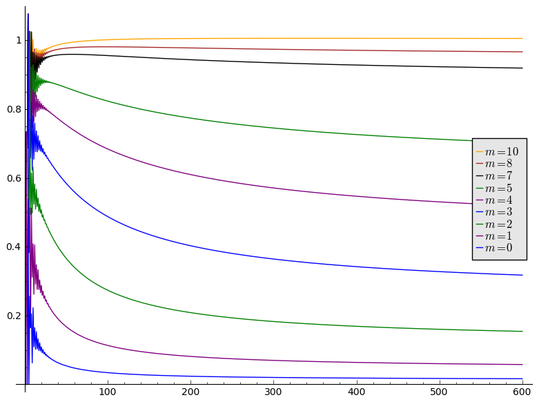
Figure 3: $S_{m,n}`r^{n}n^{3/2}$ up to $n=600$ for $m=0$ (bottom) to $10$ (top)

Conjecture 1

For every natural number $m$, we have

$$S_{m,n}\sim o\big{(}1.963448\ldots^{n}\cdot n^{-3/2}\big{)}.$$

7 Unrankings

The recurrence relation (2) for $S_{m,n}$ allows us to define the function generating $`l$-terms. More precisely, we construct bijections $s_{m,n}$, called unranking functions, between all non-negative integers not greater than $S_{m,n}$ and binary $`l$-terms of size $n$ with at most $m$ distinct free variables [14]. This approach is also known as the ‘recursive method’, originating with Nijenhuis and Wilf [19] (see especially Chapter 13).

Let us recall that for $n\geq 2$ we have, by (2),

$$S_{m,n} = [m\geq n-1]+S_{m+1,n-2}+\sum_{j=0}^{n-2}S_{m,j}S_{m,n-2-j}.$$

The encoding function $s_{m,n}$ takes an integer $k\in\{1,\ldots,S_{m,n}\}$ and returns the term built in the following way.

• If $m\geq n-1$ and $k$ is equal to $S_{m,n}$, the function returns the string $1^{n-1}0$.

• If $k$ is less than or equal to $S_{m+1,n-2}$, then the corresponding term is in the form of abstraction $00\widehat{M}$, where $\widehat{M}$ is the value of the unranking function $s_{m+1,n-2}$ on $k$.

• Otherwise, i.e., if $k$ is greater than $S_{m+1,n-2}$ and less than $S_{m,n}$ for $m\geq n+1$ or less than or equal to $S_{m,n}$ for $m<n+1$, the corresponding term is in the form of application $01\widehat{M}\widehat{N}$. In order to get strings $\widehat{M}$ and $\widehat{N}$, we compute the maximal value $\ell\in\{0,\ldots,n-2\}$ for which

  $$k-S_{m+1,n-2}=\Big{(}\sum_{j=0}^{\ell-1}S_{m,j}S_{m,n-2-j}\Big{)}+r\qquad\textrm{with~{}}\ r\leq S_{m,\ell}S_{m,n-2-\ell}.$$

  The strings $\widehat{M}$ and $\widehat{N}$ are the values $s_{m,\ell}(k^{\prime})$ and $s_{m,n-2-\ell}(k^{\prime\prime})$, respectively, where $k^{\prime}$ is the integer quotient upon dividing $r$ by $S_{m,n-2-\ell}$, and $k^{\prime\prime}$ is the remainder.

Notice that in this definition, extremal values of $k$ are considered first. Namely, first the maximal value $S_{m,n}$ (for $m\geq n-1$) is considered, then values from the set $\{1,\ldots,S_{m+1,n-2}\}$ are taken into account, and finally, in the third case, the remaining values.

In Figure 4 the reader may find a Haskell definition of the data type Term and a program [20] for computing the values $s_{m,n}(k)$. In this program, the function $s_{m,n}(k)$ is written as unrankT m n k and the sequence $S_{m,n}$ is written as tromp m n.

 

⬇

1 data Term = Index Int

2 | Abs Term

3 | App Term Term

4

5 unrankT :: Int -> Int -> Integer -> Term

6 unrankT m n k

7 | m >= n - 1 && k == (tromp m n) = Index (n - 1)

8 | k <= (tromp (m+1) (n-2)) = Abs (unrankT (m+1) (n-2) k)

9 | otherwise = unrankApp (n-2) 0 (k - tromp (m+1) (n-2))

10 where unrankApp n j r

11 | r <= tmjtmnj = let (dv,rm) = (r-1) ‘divMod‘ tmnj

12 in App (unrankT m j (dv+1))

13 (unrankT m (n-j) (rm+1))

14 | otherwise = unrankApp n (j + 1) (r -tmjtmnj)

15 where tmnj = tromp m (n-j)

16 tmjtmnj = (tromp m j) * tmnj

 

Figure 4: The data type Term and a program for computing values of the function $s_{m,n}$

8 Number of typable terms

The unranking function allows us to traverse all the closed terms of size $n$ and to filter those that are typable (see [13]) in order to count them and similarly to traverse all the terms of size $n$ to count those that are typable.

The comparison of the numbers of $`l$-terms and the numbers of typable $`l$-terms is presented in Figure 5. From left to right:

1. the numbers $S_{0,n}$ of closed terms (typable and untypable) of size $n$,

2. the numbers $T_{0,n}$ of closed typable terms of size $n$,

3. the numbers $S_{\infty,n}$ of all terms (typable and untypable) of size $n$,

4. the numbers $T_{\infty,n}$ of all typable terms of size $n$.

$\begin{array}[t]{r l}\mathbf{n}&S_{0,n}\\ \hline\cr 0&0\\ 1&0\\ 2&0\\ 3&0\\ 4&1\\ 5&0\\ 6&1\\ 7&1\\ 8&2\\ 9&1\\ 10&6\\ 11&5\\ 12&13\\ 13&14\\ 14&37\\ 15&44\\ 16&101\\ 17&134\\ 18&298\\ 19&431\\ 20&883\\ 21&1361\\ 22&2736\\ 23&4405\\ 24&8574\\ 25&14334\\ 26&27465\\ 27&47146\\ 28&89270\\ 29&156360\\ 30&293840\\ 31&522913\\ 32&978447\\ 33&1761907\\ 34&3288605\\ 35&5977863\\ 36&11148652\\ 37&20414058\\ 38&38071898\\ 39&70125402\\ 40&130880047\\ 41&242222714\\ 42&452574468\\ 43&840914719\\ 44&1573331752\\ 45&2933097201\\ 46&5495929096\end{array}\qquad\begin{array}[t]{r l}\mathbf{n}&T_{0,n}\\ \hline\cr 0&0\\ 1&0\\ 2&0\\ 3&0\\ 4&1\\ 5&0\\ 6&1\\ 7&1\\ 8&1\\ 9&1\\ 10&5\\ 11&4\\ 12&9\\ 13&13\\ 14&23\\ 15&29\\ 16&67\\ 17&94\\ 18&179\\ 19&285\\ 20&503\\ 21&795\\ 22&1503\\ 23&2469\\ 24&4457\\ 25&7624\\ 26&13475\\ 27&23027\\ 28&41437\\ 29&72165\\ 30&128905\\ 31&227510\\ 32&405301\\ 33&715078\\ 34&1280127\\ 35&2279393\\ 36&4086591\\ 37&7316698\\ 38&13139958\\ 39&23551957\\ 40&42383667\\ 41&76278547\\ 42&137609116\\ 43&248447221\\ 44&449201368\\ 45&812315229\\ 46&1470997501\\ \end{array}\qquad\qquad\begin{array}[t]{r l}\mathbf{n}&S_{\infty,n}\\ \hline\cr 0&0\\ 1&0\\ 2&1\\ 3&1\\ 4&2\\ 5&2\\ 6&4\\ 7&5\\ 8&10\\ 9&14\\ 10&27\\ 11&41\\ 12&78\\ 13&126\\ 14&237\\ 15&399\\ 16&745\\ 17&1292\\ 18&2404\\ 19&4259\\ 20&7915\\ 21&14242\\ 22&26477\\ 23&48197\\ 24&89721\\ 25&164766\\ 26&307294\\ 27&568191\\ 28&1061969\\ 29&1974266\\ 30&3698247\\ 31&6905523\\ 32&12964449\\ 33&24295796\\ 34&45711211\\ 35&85926575\\ 36&161996298\\ 37&305314162\\ 38&576707409\\ 39&1089395667\\ 40&2061428697\\ 41&3901829718\\ 42&7395529009\\ 43&14023075765\\ 44&26620080576\\ 45&50556677634\\ 46&96108150292\end{array}\qquad\begin{array}[t]{r l}\mathbf{n}&T_{\infty,n}\\[0.2pt] \hline\cr 0&0\\ 1&0\\ 2&1\\ 3&1\\ 4&2\\ 5&2\\ 6&3\\ 7&5\\ 8&8\\ 9&13\\ 10&22\\ 11&36\\ 12&58\\ 13&103\\ 14&177\\ 15&307\\ 16&535\\ 17&949\\ 18&1645\\ 19&2936\\ 20&5207\\ 21&9330\\ 22&16613\\ 23&29921\\ 24&53588\\ 25&96808\\ 26&174443\\ 27&316267\\ 28&572092\\ 29&1040596\\ 30&1888505\\ 31&3441755\\ 32&6268500\\ 33&11449522\\ 34&20902152\\ 35&38256759\\ 36&70004696\\ 37&128336318\\ 38&235302612\\ 39&432050796\\ 40&793513690\\ 41&1459062947\\ 42&2683714350\\ 43&\textit{unknown}\\ 44&\textit{unknown}\\ 45&\textit{unknown}\\ 46&\textit{unknown}\\ \end{array}$

Figure 5: Numbers of terms and numbers of typable terms

In particular, let us notice that $S_{0,n}$ and $T_{0,n}$ are the same up to $n=8$, where we meet the smallest untypable closed term namely $`l\underline{\mathsf{1}}\,\underline{\mathsf{1}}$. Similarly, $S_{\infty,n}$ and $T_{\infty,n}$ are the same up to $n=6$, where we meet the smallest untypable term, namely $\underline{\mathsf{1}}\,\underline{\mathsf{1}}$. Values $T_{\infty,43}$, $T_{\infty,44}$, $T_{\infty,45}$ and $T_{\infty,46}$ are not available since they require too many computations, between $14$ millions and $96$ millions of $`l$-terms have to be checked for typability in each case. Paul Tarau [22] gives a Prolog implementation and applies it to the generation of typed $`l$-terms.

Thanks to the unranking function, we can build a uniform generator of $`l$-terms and, using this generator, we can build a uniform generator of simply typable $`l$-terms, which sieves the uniformly generated terms through a program that checks their typability (see for instance [11]). This way, it is possible to generate typable closed terms uniformly up to size $450$.

9 Boltzmann samplers

In this section we present the basic ideas related to Boltzmann models, which combined with the theory of generating functions allow us to develop efficient algorithms for generating random $`l$-terms. A thorough and clear overview of Boltzmann samplers, including many examples, can be found in [8]. For readers not acquainted with the theory, we provide necessary notions and constructions.

Let $\mathscr{C}$ be a combinatorial class, i.e., a set of combinatorial objects endowed with a size function $|\cdot|\colon\mathscr{C}\to\mathbb{N}$ such that there are finitely many elements of size $n$ for every $n\in\mathbb{N}$. Let $C_{n}$ denote the cardinality of the subset of $\mathscr{C}$ consisting of elements of size $n$. Furthermore, let $C(z)$ denote the generating functions associated with the sequence $(C_{n})_{n\in\mathbb{N}}$, which means that

$$C(z)=\sum_{n=0}^{\infty}C_{n}z^{n}.$$

Notice that

$$C(z)=\sum_{`g`:\mathscr{C}}z^{|`g|}.$$

Given a positive real $x\in{\mathbb{R}}_{+}$, we define a Boltzmann model for the class $\mathscr{C}$ as the probability distribution that assigns to every element $\gamma\in\mathscr{C}$ a probability

$$\mathbb{P}_{\mathscr{C},x}(`g)=\frac{1}{C(x)}\cdot x^{|`g|}.$$

This is a probability since

$$\sum_{`g`:\mathscr{C}}\mathbb{P}_{\mathscr{C},x}(`g)=\sum_{`g`:\mathscr{C}}\frac{1}{C(x)}\cdot x^{|`g|}=1.$$

The role of $x$ will become clear later on, but for now we may consider $x$ as a parameter used to “tune” the sampler, that is to center the mean value around a chosen number. In other words, if we want to set an expected mean value, we have to compute the proper value of $x$. In order the probability $\mathbb{P}_{\mathscr{C},x}(`g)$ to be well-defined, we assume the values of $x$ to be taken from the interval $(0,\rho_{\mathscr{C}})$, where $\rho_{\mathscr{C}}$ denotes the radius of convergence of $C(z)$. Provided $C(z)$ converges at $\rho_{\mathscr{C}}$, we may also consider the case $x=\rho_{\mathscr{C}}$.

The size of an object in a Boltzmann model is a random variable $N$. The Boltzmann sampler for a class $\mathscr{C}$ and a parameter $x$ is a random object generator, which draws from the class $\mathscr{C}$ an object of size $n$ with probability

$$\mathbb{P}_{x}(N=n)=\frac{C_{n}x^{n}}{C(x)}.$$

This is indeed a well-defined probability since

$$\sum_{n\geq 0}\mathbb{P}_{x}(N=n)=\frac{1}{C(x)}\sum_{n\geq 0}C_{n}x^{n}=1.$$

When generating random objects, we require either the size to be a fixed value $n$ or, in order to increase the efficiency of the generation process, we admit some flexibility on the size. In other words, we want the objects to be generated in some cloud around a given size $n$ so that the size $N$ of the objects lies in some interval $(1-\varepsilon)n\leq N\leq(1+\varepsilon)n$ for some factor $\varepsilon>0$ called a tolerance. Such a method is called approximate-size uniform random generation. What we want to preserve is the uniformity of the distribution among objects of the same size, i.e., we want all objects of the same size to be drawn with the same probability.

The random variable $N$ has a first moment and a second moment [8]:

$$\mathbb{E}_{x}(N)=x\frac{C^{\prime}(x)}{C(x)}\qquad\mathbb{E}_{x}(N^{2})=\frac{x^{2}C^{\prime\prime}(x)+xC^{\prime}(x)}{C(x)},$$

and a standard deviation:

$$`s_{x}(N) = \sqrt{\mathbb{E}_{x}(N^{2})-\mathbb{E}_{x}(N)^{2}}$$

$$= \sqrt{\frac{x^{2}C^{\prime\prime}(x)+xC^{\prime}(x)}{C(x)}-x^{2}\frac{C^{\prime}(x)^{2}}{C(x)^{2}}}.$$

In the case of approximate-size generation, in order to maximize chances of drawing an object of a desired size, say $n$, we need to choose a proper value of the parameter $x$. It turns out that the best value of $x$ is such for which $\mathbb{E}_{x}(N)=n$ (for a detailed study see [9]). Given size $n$, we will denote by $x_{n}$ the value of the parameter chosen in such a way. Moreover, if $n$ tends to infinity, then $x_{n}$ tends to $\rho_{C}$ (see Appendix).

9.1 Design of Boltzmann generator

A Boltzmann generator for a class $\mathscr{C}$ is built according to a recursive specification of the class $\mathscr{C}$. Since we are interested in designing a Boltzmann sampler for binary $`l$-terms, we present the way of defining samplers for classes which are specified by means of the following recursive constructions: disjoint unions (data type Either a  b), products (data type Pair) and sequences (data type List). First we assume a monad Gen defined from the monad State of the Haskell library by

⬇

1 type Gen = State StdGen

where StdGen is the type of standard random generators. For the following we assume a function rand :: Gen Double that generates a random double precision real in the interval $(0,1)$ together with an update of the random generator. In our case it is defined in Figure 6.

⬇

1 rand :: Gen Double

2 rand = do generator <- get

3 let (value, newGenerator) = randomR (0,1) generator

4 put newGenerator

5 return value

Figure 6: The function rand

9.2 Disjoint union

Let a and b be two types (corresponding to combinatorial classes $\mathscr{A}$ and $\mathscr{B}$). A generator genEither for the disjoint union takes a double precision number for the Bernoulli choice and two objects of type Gen a and Gen b and returns an object of type Gen ( Either a b). If we define a new class as c = Either a b corresponding to the class $\mathscr{C}$ with the size function inherited from classes $\mathscr{A}$ and $\mathscr{B}$, then $C_{n}=A_{n}+B_{n}$ and $C(z)=A(z)+B(z)$. The probability of drawing an object $\gamma\in\mathscr{C}$ equals

$$\mathbb{P}_{\mathscr{C},x}(`g`:\mathscr{A})=\frac{A(x)}{C(x)},\qquad\mathbb{P}_{\mathscr{C},x}(`g`:\mathscr{B)}=\frac{B(x)}{C(x)}.$$

A generator for the disjoint union, i.e., a Bernoulli variable, may have the following type:

⬇

1 genEither::Double -> (Gen a) -> (Gen b) -> (Either a b -> c) -> Gen c

and then it is given by the Haskell function:

⬇

1 genEither p ga gb caORb = do

2 x <- rand

3 if x < p then do ga’ <- ga

4 return (caORb $ Left ga’)

5 else do gb’ <- gb

6 return (caORb $ Right gb’)

Notice the type of genEither which assumes that genEither takes a number, two monad values Gen a and Gen b (which can be seen as pairs of a random generator and a value of type a and b respectively), and a continuation c of type Either a b and returns a value of the monad Gen c. Similar frames will appear in the programs describing other generators.

9.3 Cartesian product

Given classes $\mathscr{A}$ and $\mathscr{B}$, let $\mathscr{C}$ be the class defined as their Cartesian product, i.e., $\mathscr{C}=\mathscr{A}\times\mathscr{B}$. Let a and b be Haskell types corresponding to classes $\mathscr{A}$ and $\mathscr{B}$. Then the type of the class $\mathscr{C}$ is $\mathtt{(a,b)}$. The size of an object $\gamma=\langle\alpha,\beta\rangle\in\mathscr{C}$ equals the sum of sizes $|\alpha|+|\beta|$. In more concrete terms, if an object is the pair of an object of size $p$ and an object of size $q$, then its size is $p+q$. Hence, the generating functions satisfy the equation $C(z)=A(z)\cdot B(z)$, since

$$C(z)=\sum_{\langle`a,`b\rangle`:\mathscr{A}\times\mathscr{B}}z^{|`a|+|`b|}.$$

The probability of drawing $`g=\langle`a,`b\rangle`:\mathscr{C}$ is equal to

$$\mathbb{P}_{\mathscr{C},x}(`g)=\frac{x^{|`g|}}{C(x)}=\frac{x^{|`a+`b|}}{A(x)\cdot B(x)}=\frac{x^{|`a|}}{A(x)}\cdot\frac{x^{|`b|}}{B(x)}.$$

In this case the Boltzmann sampler is as follows:

⬇

1 genPair :: (Gen a) -> (Gen b) -> (a -> b -> c) -> (Gen c)

2 genPair ga gb caANDb = do

3 ga’ <- ga

4 gb’ <- gb

5 return (caANDb ga’ gb’)

10 Boltzmann samplers for $`l$-terms

Let us consider the equation involving the generating function for all $`l$-terms:

$$S_{\infty}(z)=\frac{z^{2}}{1-z}+z^{2}S_{\infty}(z)+z^{2}S_{\infty}(z)^{2}.$$

It is derived from the description of the set $\mathscr{S}_{\infty}$ of $`l$-terms as:

$$\mathscr{S}_{\infty}=\mathscr{D}+`l\mathscr{S}_{\infty}+\mathscr{S}_{\infty}\,\mathscr{S}_{\infty}.$$

That means that the set of $`l$-terms $\mathscr{S}_{\infty}$ has three components: the first component $\mathscr{D}$ corresponds to de Bruijn indices, the second component $`l\mathscr{S}_{\infty}$ corresponds to abstractions, the third component $\mathscr{S}_{\infty}\mathscr{S}_{\infty}$ corresponds to applications. We build a sampler of random terms based on this trichotomy. In Haskell this corresponds to a data type Term defined in Figure 4. Since there are three components in the union, the value $\mathtt{p}$ which we considered in $\mathtt{genEither}$ will be replaced by two values $\mathtt{p1}$ and $\mathtt{p2}$. First we describe in Haskell a function corresponding to $S_{\infty}(z)$:

⬇

1 sInfinity z = num z / den z

2 where num z = z^3 - z^2 - z + 1 - sqrt(sq z)

3 den z = 2*z*z*(1 - z)

4 sq z = z^6 + 2*(z^5) - 5*(z^4) + 4*(z^3) - z^2 - 2*z + 1

and two functions:

⬇

1 p1 x = x*x / (1-x) / sInfinity x

2 p2 x = p1 x + x^2

Using Sage we computed the values:

$$x_{100}\,=\,0.5092252666102192\quad x_{600}\,=\,0.5093058457062517\quad x_{1000}\,=\,0.5093073063214039$$

which correspond to the values of the parameter $x$ appropriate for an expected value $\mathbb{E}_{x_{i}}(N)$ equal to $i=100$, $i=600$, and $i=1000$, respectively. In other words if the values $x_{100}$, $x_{600}$ and $x_{1000}$ are passed to the sampler, it will generate objects with average size $100$, $600$, and $1000$, respectively. They are obtained by solving in $x$ the equations

$$\mathbb{E}_{x}(N) = 100,$$

$$\mathbb{E}_{x}(N) = 600,$$

$$\mathbb{E}_{x}(N) = 1000,$$

in which $C(x)$ is replaced by $S_{\infty}(x)$.

10.1 General samplers of $`l$-terms

The values of the probabilities for a given $x$ are

• $p_{v}(x)=\frac{x^{2}}{(1-x)S_{\infty}(x)}$ for variables,

• $p_{abs}(x)=x^{2}$ for abstractions,

• $p_{app}(x)=x^{2}S_{\infty}(x)$ for applications.

We get the following Haskell function which selects among Index, Abs and App

⬇

1 genTermGeneric :: Double -> Gen Int -> Gen Term

2 genTermGeneric x gi = do

3 p <- rand

4 if p < p1 x

5 then do i <- genIntGeneric x

6 return (Index i)

7 else if p < p2 x

8 then do t <- genTermGeneric x gi

9 return (Abs t)

10 else genPair (genTermGeneric x gi) (genTermGeneric x gi) App

Notice the call to the function

⬇

1 genIntGeneric :: Double -> Gen Int

2 genIntGeneric x = do

3 p <- rand

4 if p < x then do n <- genIntGeneric x

5 return (n+1)

6 else return 1

which is used to generate random de Bruijn indices.

10.2 Samplers for large $`l$-terms

⬇

1 rho :: Double

2 rho = 0.509308127024237357194177485

3 rhosquare = rho * rho

4 p1rho = (1 - rhosquare) / 2

5 p2rho = p1rho + rhosquare

6

7 genTerm :: Gen Int -> Gen Term

8 genTerm gi = do

9 p <- rand

10 if p < p1rho then do i <- genInt

11 return (Index i)

12 else if p < p2rho

13 then do t <- genTerm gi

14 return (Abs t)

15 else genPair (genTerm gi) (genTerm gi) App

16

17 genInt :: Gen Int

18 genInt = do

19 p <- rand

20 if p < rho then do n <- genInt

21 return (n+1)

22 else return 1

Figure 7: The function genTerm

As discussed in the previous section, in order to generate random large $\lambda$-terms, i.e., $`l$-terms with average size $\infty$, we set the value of $x$ to $\rho=0.5093081270242373\ldots$, which we call rho in Haskell. Its square is

$$`r^{2}=0.25939476825293667\ldots.$$

Notice that since $`r$ is a root of the polynomial below the square root, $S_{\infty}(`r)=\frac{1-`r^{2}}{2`r^{2}}$. The values of the probabilities for selecting among variables, abstractions and applications are:

• $p_{v}(`r)=\frac{2`r^{4}}{(1-`r)(1-`r^{2})}$  for variables,

• $p_{abs}(`r)=`r^{2}$  for abstractions,

• $p_{app}(`r)=\frac{1-`r^{2}}{2}$  for applications.

Let us simplify $\frac{2`r^{4}}{(1-`r)(1-`r^{2})}$ into $\frac{1-`r^{2}}{2}$ by computing the difference:

$$\frac{2`r^{4}}{(1-`r)(1-`r^{2})}-\frac{1-`r^{2}}{2} = \frac{4`r^{4}-(1-`r^{2})^{2}(1-`r)}{2(1-`r)(1-`r^{2})}$$

$$= \frac{`r^{5}+3`r^{4}-2`r^{3}+2`r^{2}+`r-1}{2(1-`r)(1-`r^{2})}\,=\,0.$$

Therefore to generate random terms of mean size going to infinity we get the results

• $p_{v}(`r)=\frac{1-`r^{2}}{2}\approx 0.3703026$  for variables,

• $p_{abs}(`r)=`r^{2}\approx 0.25939476$  for abstractions,

• $p_{app}(`r)=\frac{1-`r^{2}}{2}\approx 0.3703026$  for applications.

We build the function genTerm which generates random terms and the function genInt which generates integers necessary for the de Bruijn indices (see Figure 7). The list

$$60,5,3,3,6,19,8,7,728,3753,12,15,3733,93,4,3,4,4,13,137,6,18,372,50,25,43140,8,5,3,6$$

is the list of term sizes generated by genTerm when the seeds of the random generator are $0,1,2,\ldots$ up to $30$. In the same list of term sizes the $50^{th}$ element is $127\,358$ and the $51^{st}$ element is $4\,379\,394$, showing that generating a random term of size more than four million is easy.

Assume now that we want to generate terms that are below a certain uplimit, as required by practical applications. The function called ceiledGenTerm is almost the same as genTerm, except that when the up limit is passed it returns Nothing. Therefore the type of ceiledGenTerm differs from genTerm type in the sense that it takes a Gen (Maybe Term) (instead of a Gen Term) and returns a Gen (Maybe Term) (instead of a Gen Term). A Boltzmann sampler ceiledGenTerm for large $`l$-terms of size limited by uplimit is given in Figure 8.

⬇

1 ceiledGenTerm :: Int -> Gen Int -> Gen (Maybe Term)

2 ceiledGenTerm uplimit gi = do

3 p <- rand

4 if p < p1rho

5 then do – generate an index

6 i <- genInt

7 return $ if i < uplimit then Just (Index i) else Nothing

8 else if p < p2rho

9 then do – generate an abstraction

10 mbt <- ceiledGenTerm uplimit gi

11 return $ case mbt of

12 Just t -> if 2 + size t <= uplimit

13 then Just (Abs t)

14 else Nothing

15 Nothing -> Nothing

16 else do – generate an application

17 mbt1 <- ceiledGenTerm uplimit gi

18 mbt2 <- ceiledGenTerm uplimit gi

19 return $ case mbt1 of

20 Just t1 -> case mbt2 of

21 Just t2 -> if 2 + size t1 + size t2 <= uplimit

22 then Just (App t1 t2)

23 else Nothing

24 Nothing -> Nothing

Figure 8: Boltzmann sampler for large $`l$-terms

Suppose now that we want to generate terms within a size interval, i.e., with an up limit and a down limit. By definition, ceiledGenTerm generates terms within an up limit. For terms within the down limit, terms generated by ceiledGenTerm are filtered so that only terms large enough are kept. Recall that the method is linear in time complexity. Thus the generation of a term of size $100\,000$ takes a few seconds, the generation of a term of size one million takes three minutes and the generation of a term of size five million takes five minutes.

To generate large typable $`l$-terms we generate $`l$-terms and check their typability. Currently we are able to generate random typable $`l$-terms of size $500$. This outperforms methods based on ranking and unranking like the method proposed in [11]. This is in particular due to the fact that such methods need to handle numbers of arbitrary precision and their random generation, which it not efficient. Indeed ranking or unranking requires handling integers with hundred digits or more and performing computations on them for their random generations. On the other hand, Boltzmann samplers ignore numbers, go directly toward the terms to be generated and do that efficiently.

11 Related works

We look at related works from two perspectives: works on counting $`l$-terms and works specifically related to Boltzmann samplers.

11.1 Works on counting $`l$-terms

Connected to this work, let us mention papers on counting $`l$-terms [17, 11] and on evaluating their combinatorial properties, namely [2, 6, 3, 4]. A comparison of our results with those of [11] can be made, since [11] gives a precise counting of $`l$-terms when variables (de Bruijn indices) have size $0$, yielding sequence A220894 in the On-line Encyclopedia of Integer Sequences for the number of closed terms of size $n$. The first fifteen terms are:

$0,\ 1,\ 3,\ 14,\ 82,\ 579,\ 4741,\ 43977,\ 454283,\ 5159441,\ 63782411,\ 851368766,$

$12188927818,\ 186132043831,\ 3017325884473.$

If one compares them with the first fifteen terms of $S_{0,n}$:

$$0,\ 0,\ 0,\ 0,\ 1,\ 0,\ 1,\ 1,\ 2,\ 1,\ 6,\ 5,\ 13,\ 14,\ 37,$$

one sees that $S_{0,n}$ grows much more slowly than A220894, which is not surprising since $S_{0,n}$ grows exponentially, whereas A220894 grows super-exponentially (the radius of convergence of its generating function is $0$). This super-exponential growth and the related $0$ radius of convergence prevent from building a Boltzmann sampler. Moreover, it does not make sense to count all (including open) terms of size $n$ when variables have size $0$ for the reason that there are infinitely many such terms for each $n$. Notice that taking the size of variables to be $1$, like [17, 2], does not make much difference for growth and generation.

11.2 Works related to Boltzmann samplers for terms

In the introduction we cited papers that are clearly connected to this work. In a recent work, Bacher et al. [1] propose an improved random generation of binary trees and Motzkin trees, based on Rémy algorithm [21] (or algorithm R in Knuth [15]). They propose like Rémy to grow the trees from inside by an operation called grafting. It is not clear how this can be generalized to $`l$-terms as one needs “to find a combinatorial interpretation for the holonomic equations [which] is not […] always possible, and even for simple combinatorial objects this is not elementary” (Conclusion of [1] page 16).

12 Conclusion

We have shown that if the size of a lambda term is yielded by its binary representation [23], we get an exponential growth of the sequence enumerating $`l$-terms of a given size. This applies to closed $`l$-terms, to $`l$-terms with a bounded number of free variables, and to all $`l$-terms of size $n$. Except for the case of all $`l$-terms, the question of finding the non-exponential factor of the asymptotic approximation of the numbers of those terms is still open. Moreover, we have described unranking functions (recursive methods) for generating $`l$-terms, which allow us to derive tools for their uniform generation and for enumeration of typable $`l$-terms. The process of generating random (typable) terms is limited by the performance of the generators based on the recursive methods aka unranking since huge numbers are involved. It turns out that implementing Boltzmann samplers, central tools for the uniform generation of random structures such as trees or $`l$-terms, gives significantly better results. There are now two directions for further development: the first one consists in integrating the programs proposed here in actual testers and optimizers [5] and the second one in extending Boltzmann samplers to other kinds of programs, for instance programs with block structures. From the theoretical point of view, more should be known about generating functions for closed $`l$-terms or $`l$-terms with fixed bounds on the number of free variables. Boltzmann samplers should be designed for such terms, which requires extending the theory. As concerns combinatorial properties of simply typable $`l$-terms, many question are left open and seem to be hard. Besides, since we are interested in generating typable terms, it is worth designing random uniform samplers that deliver typable terms directly.

Acknowledgements

The authors are happy to acknowledge people who commented early versions of this paper, and contributed to improve it, especially the editors and the referees of the Journal of Functional Programming and of the 25th International Conference on Probabilistic, Combinatorial and Asymptotic Methods for the Analysis of Algorithms. The authors would like to give special mentions to Olivier Bodini, Bernhard Gittenberger, Éric Fusy, Patrik Jansson, Marek Zaionc and the participants of the 8th Workshop on Computational Logic and Applications.

The case $x=`r_{\mathscr{C}}$: generating objects with mean size $\infty$

In this section we show that choosing a value $x=`r_{\mathscr{C}}$ for the parameter of a sampler yields mean size $\infty$ of the generated objects.

Assume that a generating function we consider is of the form:

$$C(x)=\frac{P_{C}(x)-\sqrt{Q_{C}(x)}}{R_{C}(x)},$$

where $P_{C}(x)$, $Q_{C}(x)$ and $R_{C}(x)$ are three polynomials and where $`r_{\mathscr{C}}$ is such that ${Q_{C}(`r_{\mathscr{C}})=0}$ and where $Q_{C}(x)>0$ and $R_{C}(x)\neq 0$ for $0<x<`r_{\mathscr{C}}$. Those properties are fulfilled by the generating function $S_{\infty}(x)$. Indeed,

$$P_{S_{\infty}}(z) = (1-z)(1-z^{2}),$$

$$Q_{S_{\infty}}(z) = (1-z)(1-z-2\,z^{2}+2\,z^{3}-3\,z^{4}-z^{5}),$$

$$R_{S_{\infty}} = 2z^{2}(1-z).$$

Notice that $Q^{\prime}_{C}(`r_{\mathscr{C}})<0$ in the vicinity of $`r_{\mathscr{C}}$, i.e., in an interval $(`r_{\mathscr{C}}-\varepsilon,`r_{\mathscr{C}})$ (because $Q_{C}(`r_{\mathscr{C}})=0$ and $Q_{C}(x)>0$ for $x`:(0,`r_{\mathscr{C}}]$) and

$$C(`r_{\mathscr{C}})=\frac{P_{C}(`r_{\mathscr{C}})}{R_{C}(`r_{\mathscr{C}})}$$

is finite. On the other hand,

$$C^{\prime}(x)=\frac{P^{\prime}_{C}(x)}{R_{C}(x)}-\frac{Q^{\prime}_{C}(x)}{2\sqrt{Q_{C}(x)}R_{C}(x)}-\frac{(P_{C}(x)-\sqrt{Q_{C}(x)})R^{\prime}_{C}(x)}{R_{C}(x)^{2}}$$

shows that

$$\lim_{x"->"`r_{\mathscr{C}}}C^{\prime}(x)=\infty.$$

Hence

$$\lim_{x"->"`r_{\mathscr{C}}}\mathbb{E}_{x}(N)=\lim_{x"->"`r_{\mathscr{C}}}\frac{xC^{\prime}(x)}{C(x)}=\infty.$$

Therefore, if we choose $x$ to be $`r_{\mathscr{C}}$, the size of the generated structures will be distributed all over the natural numbers, with an infinite average size.

References

- [1] Axel Bacher, Olivier Bodini, and Alice Jacquot. Efficient random sampling of binary and unary-binary trees via holonomic equations. CoRR, abs/1401.1140, 2014.
- [2] Olivier Bodini, Danièle Gardy, and Bernhard Gittenberger. Lambda-terms of bounded unary height. 2011 Proceedings of the Eighth Workshop on Analytic Algorithmics and Combinatorics (ANALCO), 2011.
- [3] Olivier Bodini, Danièle Gardy, Bernhard Gittenberger, and Alice Jacquot. Enumeration of generalized BCI lambda-terms. Electr. J. Comb., 20(4):P30, 2013.
- [4] Olivier Bodini, Danièle Gardy, and Alice Jacquot. Asymptotics and random sampling for BCI and BCK lambda terms. Theor. Comput. Sci., 502:227–238, 2013.
- [5] Koen Claessen and John Hughes. QuickCheck: a lightweight tool for random testing of Haskell programs. In Martin Odersky and Philip Wadler, editors, ICFP, pages 268–279. ACM, 2000.
- [6] René David, Katarzyna Grygiel, Jakub Kozik, Christophe Raffalli, Guillaume Theyssier, and Marek Zaionc. Asymptotically almost all -terms are strongly normalizing. Logical Methods in Computer Science, 9(1:02):1–30, 2013.
- [7] Nicolaas G. de Bruijn. Lambda calculus notation with nameless dummies, a tool for automatic formula manipulation, with application to the Church-Rosser theorem. Indagationes Mathematicae, 34(5):381–392, 1972.
- [8] Philippe Duchon, Philippe Flajolet, Guy Louchard, and Gilles Schaeffer. Boltzmann samplers for the random generation of combinatorial structures. Combinatorics, Probability & Computing, 13(4-5):577–625, 2004.
- [9] Philippe Flajolet, Éric Fusy, and Carine Pivoteau. Boltzmann sampling of unlabeled structures. In Proceedings of the Fourth Workshop on Analytic Algorithmics and Combinatorics, ANALCO 2007, New Orleans, Louisiana, USA, January 06, 2007, pages 201–211, 2007.
- [10] Philippe Flajolet and Robert Sedgewick. Analytic Combinatorics. Cambridge University Press, 2008.
- [11] Katarzyna Grygiel and Pierre Lescanne. Counting and generating lambda terms. Journal of Functional Programming, 23(5):594–628, 2013.
- [12] Katarzyna Grygiel and Pierre Lescanne. Counting terms in the binary lambda calculus. CoRR, abs/1401.0379, 2014. Published in the Proceedings of 25th International Conference on Probabilistic, Combinatorial and Asymptotic Methods for the Analysis of Algorithms 2014, https://hal.inria.fr/hal-01077251.
- [13] J. Roger Hindley. Basic Simple Type Theory. Number 42 in Cambridge Tracts in Theoretical Computer Science. Cambridge University Press, 1997.
- [14] Antti Karttunen. Ranking and unranking functions. OEIS Wiki, 2015. http://oeis.org/wiki/Ranking_and_unranking_functions.
- [15] Donald E. Knuth. The Art of Computer Programming, Volume 4, Fascicle 4: Generating All Trees, History of Combinatorial Generation (Art of Computer Programming). Addison-Wesley, 2006.
- [16] Pierre Lescanne. From to , a journey through calculi of explicit substitutions. In Hans Boehm, editor, Proceedings of the 21st Annual ACM Symposium on Principles Of Programming Languages, Portland (Or., USA), pages 60–69. ACM, 1994.
- [17] Pierre Lescanne. On counting untyped lambda terms. Theoretical Computer Science, 474:80–97, 2013.
- [18] Ming Li and Paul Vitányi. An introduction to Kolmogorov complexity and its applications (3rd ed.). Springer-Verlag New York, Inc., 2008.
- [19] Albert Nijenhuis and Herbert S. Wilf. Combinatorial algorithms, 2nd edition. Computer science and applied mathematics. Academic Press, New York, 1978.
- [20] Simon Peyton Jones, editor. Haskell 98 language and libraries: the Revised Report. Cambridge University Press, 2003.
- [21] Jean-Luc Rémy. Un procédé itératif de dénombrement d’arbres binaires et son application à leur génération aléatoire. ITA, 19(2):179–195, 1985.
- [22] Paul Tarau. On type-directed generation of lambda terms. In 31st International Conference on Logic Programming (ICLP 2015), 2015.
- [23] John Tromp. Binary lambda calculus and combinatory logic. In Marcus Hutter, Wolfgang Merkle, and Paul M. B. Vitányi, editors, Kolmogorov Complexity and Applications, volume 06051 of Dagstuhl Seminar Proceedings. Internationales Begegnungs- und Forschungszentrum fuer Informatik (IBFI), Schloss Dagstuhl, Germany, 2006.
- [24] Jue Wang. The efficient generation of random programs and their applications. Honors Thesis, Wellesley College, Wellesley, MA, May 2004.