Low-field behavior of an $XY$ pyrochlore antiferromagnet: emergent clock anisotropies

Abstract

Using $\rm Er_{2}Ti_{2}O_{7}$ as a motivation, we investigate finite-field properties of $XY$ pyrochlore antiferromagnets. In addition to a fluctuation-induced six-fold anisotropy present in zero field, an external magnetic field induces a combination of two-, three-, and six-fold clock terms as a function of its orientation providing for a rich and controllable magnetothermodynamics. For $\rm Er_{2}Ti_{2}O_{7}$, we predict a new phase transition for ${\bf H}\parallel[001]$. Re-entrant transitions are also found for ${\bf H}\parallel[111]$. We extend these results to the whole family the $XY$ pyrochlore antiferromagnets and show that presence and number of low-field transitions for different orientations can be used for locating a given material in the parameter space of anisotropic pyrochlores. Finite-temperature classical Monte Carlo simulations serve to confirm and illustrate these analytic predictions.

The Ising model is commonly used to describe the $Z_{2}$ symmetry breaking for a wide range of physical systems including simple magnets, lattice gases, and neural networks Chaikin_Lubensky ; Schneidman06 . Its well-known generalizations are provided by models with $Z_{N}$ symmetry: Potts and clock models. Being abundantly investigated for their own sake, these models and the related symmetry breaking transitions Jose77 rarely appear in studies of real magnetic materials. Yet an interesting example of a $Z_{6}$ clock anisotropy was recently identified for the ordering transition in the $XY$ pyrochlore antiferromagnet $\rm Er_{2}Ti_{2}O_{7}$ Champion03 ; Champion04 ; Poole07 ; MZ12 ; Savary12 ; Wong13 ; Yan13 ; MZ14 ; Ross14 ; McClarty14 ; Petit14 ; Javanparast15 and in two other members of this family Li14 ; Dun15 . A characteristic feature of an antiferromagnet with Ising anisotropy is the spin-flop transition in a magnetic field applied along the easy (Ising) axis Majlis . Field-induced transitions in magnets with broken $Z_{N}$ symmetry are much less documented. Therefore, understanding the interplay between the discrete $Z_{6}$ symmetry and an external field in the $XY$ pyrochlore antiferromagnets is of significant interest from a general perspective.

$\rm Er_{2}Ti_{2}O_{7}$ is the most studied $XY$ pyrochlore antiferromagnet. It orders into a four-sublattice noncoplanar magnetic structure called the $\psi_{2}$ state Champion03 ; Poole07 . Together with a companion $\psi_{3}$ magnetic structure, see Fig. 1, the two states transform according to the $\Gamma_{5}$ ($E$) representation of the tetrahedral point group $T_{d}$. They remain degenerate at the mean-field level signifying an emergent $U(1)$ symmetry revealed, e.g., in the critical behavior MZ14 . The experimentally observed stabilization of the $\psi_{2}$ over the $\psi_{3}$ spin configuration was attributed to an ‘order by disorder’ effect produced by quantum and thermal fluctuations, which generate an effective six-fold anisotropy in the $U(1)$ manifold spanned by the $\psi_{2,3}$ states Champion03 ; MZ12 ; Savary12 ; Wong13 . An alternative mechanism based on virtual crystal-field excitations also favors the $\psi_{2}$ state Petit14 ; Mcclarty09 ; Rau15 . It remains unclear at present which microscopic process dominates in $\rm Er_{2}Ti_{2}O_{7}$ and, in view of the $\psi_{3}$ magnetic structure found in $\rm Er_{2}Ge_{2}O_{7}$ Dun15 , if the selection mechanism varies across the pyrochlore family.

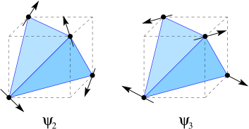
Figure 1: (Color online) The basis magnetic structures of the $\Gamma_{5}$-ordered $XY$ pyrochlores: the noncoplanar $\psi_{2}$ ($m_{1}$) state appearing in $\rm Er_{2}Ti_{2}O_{7}$ in a zero field and the coplanar $\psi_{3}$ ($m_{2}$) state.

In this Rapid Communication, we investigate the effect of an arbitrarily oriented field on the magnetic structure in $\Gamma_{5}$-ordered $XY$ pyrochlores. The developed theory does not depend on the specific mechanism that breaks degeneracy between $\psi_{2}$ and $\psi_{3}$ states in zero field and is applicable for both signs of the effective six-fold anisotropy. Field-induced anisotropic terms compete with the zero-field selection and produce orientation-dependent phase transitions. The corresponding critical fields quantify strength of the six-fold anisotropy in zero field, which was so far assessed only via the spin gap measurements Ross14 ; Petit14 . Furthermore, using information about the number of phase transitions taking place for different field orientations one can unambiguously determine the sign of the zero-field anisotropy and position a given material on the generalized phase diagram of anisotropic pyrochlore antiferromagnets Wong13 ; Savary12b ; Yan13 .

The minimal model for $\rm Er_{2}Ti_{2}O_{7}$ and other $XY$ pyrochlores with Kramers magnetic ions is an effective spin-1/2 Hamiltonian

$$\hat{\cal H} = \sum_{\langle ij\rangle}\bigl{[}J_{\perp}{\bf S}^{\perp}_{i}\cdot{\bf S}^{\perp}_{j}+J_{\perp}^{a}({\bf S}^{\perp}_{i}\cdot\hat{\bf r}_{ij})({\bf S}^{\perp}_{j}\cdot\hat{\bf r}_{ij})\bigr{]}$$ (1)

$$\mbox{}-\mu_{B}\!\sum_{i}g_{\alpha\beta}H^{\alpha}S_{i}^{\beta}\,.$$

with exchange ($J_{\perp}$) and pseudodipolar ($J_{\perp}^{a}$) interactions between spin components orthogonal to the local trigonal axes $\hat{\bf z}_{i}$ MZ12 . Here, $\hat{\bf r}_{ij}$ denotes bond direction, and $g_{\alpha\beta}$ is a staggered $g$-tensor with diagonal values $g_{z}$ and $g_{\perp}$. Additional omitted terms that involve $S_{i}^{z}$ components are smaller by about an order of magnitude MZ14 ; Savary12 . We also exclude from (1) multi-spin interactions generated by crystal-field fluctuations Rau15 . By fitting the low-$T$ magnetization data for $\rm Er_{2}Ti_{2}O_{7}$ Bonville13 , we obtain $J_{\perp}=0.2$ meV, $J_{\perp}^{a}=0.3$ meV, $g_{\perp}=6$, and $g_{z}/g_{\perp}\simeq 0.5$. These values agree within 10–15 % with the previous estimates Savary12 ; Petit14 and give good magnetization fits, see Supplemental Material for extra details Suppl .

Projections of a given spin configuration onto two basis states of the $\Gamma_{5}$ representation denoted as $m_{1}$ ($\psi_{2}$) and $m_{2}$ ($\psi_{3}$) form a two-component order parameter. At the mean-field level, the bilinear spin Hamiltonian (1) leaves a continuous degeneracy within the $\Gamma_{5}$-manifold of magnetic states. The classical energy remains the same for an arbitrary superposition of $\psi_{2}$ and $\psi_{3}$ states characterized by $m_{1}\cos\varphi+m_{2}\sin\varphi$, thus featuring an “accidental” $U(1)$ symmetry. The complex combinations $m_{\pm}=m_{1}\pm im_{2}=me^{\pm i\varphi}$ transform under $T_{d}$ symmetry operations as

$$\hat{C}_{3}^{[111]}m_{\pm}=e^{\mp 2\pi i/3}m_{\pm}\,,\quad\hat{\sigma}_{d}^{[110]}m_{\pm}=m_{\mp}\,.$$ (2)

Allowed terms in the Landau functional correspond to invariants constructed from $m_{1},m_{2}$ that are also symmetric under time-reversal. The $\varphi$-dependent terms lift the $U(1)$ degeneracy. In zero field, the leading degeneracy-breaking term appears at sixth order:

$$E_{6}[{\bf m}]=-\frac{a_{6}}{2}(m_{+}^{6}+m_{-}^{6})=-A_{6}\cos 6\varphi\,.$$ (3)

It is produced by a combined effect of quantum, thermal, and crystal-field fluctuations. Specifically, the quantum spin-wave contribution can be represented by the lowest harmonics (3) with

$$A_{6}=\frac{2J_{\perp}+J_{\perp}^{a}}{288}\,\epsilon^{3}SN\,,\quad\epsilon=\frac{J_{\perp}-\frac{1}{4}J_{\perp}^{a}}{J_{\perp}+\frac{1}{2}J_{\perp}^{a}}\,,$$ (4)

where $S=1/2$ and $N$ is the total number of sites Maryasin14 . For $J_{\perp}^{a}/J_{\perp}<4$, $A_{6}$ is positive selecting the $\psi_{2}$ states ($\varphi_{n}=\pi n/3$), whereas for $J_{\perp}^{a}/J_{\perp}>4$ the quantum correction stabilizes the $\psi_{3}$ states ($\varphi_{n}=\pi(n+\frac{1}{2})/3$).

Applying the symmetry rules (2) one can also construct energy invariants in a finite magnetic field. The lowest-order invariant is

$$E_{2}[{\bf m},{\bf H}]=\frac{a_{2}}{2}\bigl{[}m_{+}^{2}\bigl{(}e^{2\pi i/3}H_{x}^{2}+e^{-2\pi i/3}H_{y}^{2}+H_{z}^{2}\bigr{)}+\textrm{c.c.}\bigr{]}\,.$$ (5)

An external field induces a $2\varphi$-harmonic in the angular-dependent part of the free energy. For ${\bf H}\parallel[001]$ and ${\bf H}\parallel[110]$, the expression (5) is further simplified to

$$E_{2}^{[001]}=A_{2}H^{2}\cos 2\varphi\,,\quad E_{2}^{[110]}=-\textstyle{\frac{1}{2}}A_{2}H^{2}\cos 2\varphi\,.$$ (6)

The anisotropy has opposite signs for the two orientations, leading to different sequences of field-induced phases and transitions.

Direct minimization of the classical energy (1) yields

$$A_{2}=\frac{(g_{\perp}\mu_{B})^{2}N}{8(2J_{\perp}+J^{a}_{\perp})}\,.$$ (7)

Since $A_{2}>0$, the sole effect of magnetic field ${\bf H}\parallel[110]$ for $\rm Er_{2}Ti_{2}O_{7}$ is to select two domains of the $\psi_{2}$ state with $\varphi=0,\pi$. The two degenerate states smoothly evolve in an increasing field up to the transition into a ‘fully polarized’ state at $H=H_{s}$, as was observed in the neutron experiments Ruff08 ; Cao10 . In contrast, for ${\bf H}\parallel[001]$, the field-induced anisotropy $E_{2}$ competes with the zero-field term (3) producing an extra transition at $H_{c}=3\sqrt{A_{6}/A_{2}}$.

Generally, an applied field tilts magnetic moments from the respective easy planes and admixes other irreducible representations. These effects are, however, small once the magnetic field is weak $H_{c}\ll H_{s}$, which is guaranteed by small $A_{6}$. Accordingly, we represent transformation of the magnetic structure in a weak field by a dot position on a circle showing the evolution within the $U(1)$-manifold of $\Gamma_{5}$-states, see Fig. 2. In particular, below $H_{c}$, there are four magnetic domains described by $4\cos^{2}\!2\varphi=1+A_{2}H^{2}/(3A_{6})$. The broken rotational symmetry is partially restored at $H=H_{c}$ and there remain only two equilibrium states with $\varphi=\pm\pi/2$. These nearly coplanar $\psi_{3}$ magnetic structures lie in the plane orthogonal to the field direction similar to the canted spin-flop state of ordinary antiferromagnets.

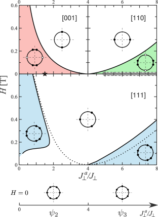
Figure 2: Color online) Low-field transitions in the $XY$ pyrochlore antiferromagnet at $T=0$ as a function of $J_{\perp}^{a}/J_{\perp}$ ($J_{\perp}=0.2$ meV, $g_{\perp}=6$). Top panels: ${\bf H}\parallel[001]$ and [110]; intermediate panel: ${\bf H}\parallel[111]$. Circles with full dots show the $U(1)$ manifold of $\Gamma_{5}$ states with equilibrium values of angle $\varphi$. Light dots denote energetically unfavorable domains. A star on the $J_{\perp}^{a}/J_{\perp}$ axis indicates the parameter ratio appropriate for $\rm Er_{2}Ti_{2}O_{7}$. The shaded area for $J_{\perp}^{a}/J_{\perp}>4$ shows the parameter region proposed for $\rm Er_{2}Ge_{2}O_{7}$ and $\rm Yb_{2}Ge_{2}O_{7}$. The dotted line corresponds to a single transition exhibited by the classical model.

We use the full expression for the field-induced anisotropy to calculate $H_{c}$ versus $J_{\perp}^{a}/J_{\perp}$ under assumption that quantum effects are dominant, see Suppl for further details. Results shown in the top-left panel of Fig. 2 were obtained with $J_{\perp}=0.2$ meV and $g_{\perp}=6$. For $\rm Er_{2}Ti_{2}O_{7}$, the transition into the $\psi_{3}$ state takes place in a rather weak field $H_{c}\approx 0.2$ T compared to $H_{s}=1.7$ T. Smallness of $H_{c}$ reflects the strength of the order by disorder effect and justifies the above assumptions. By measuring $H_{c}$ in $\rm Er_{2}Ti_{2}O_{7}$, it is possible to verify presence of other contributions to $E_{6}$ produced, e.g., by virtual crystal-field excitations Petit14 ; Rau15 .

For $J_{\perp}^{a}/J_{\perp}>4$, the quantum anisotropy (3) changes sign. Accordingly, the behavior is interchanged between the two field orientations: continuous evolution is found for ${\bf H}\parallel[001]$, whereas an extra transition into the $\psi_{2}$ state occurs for ${\bf H}\parallel[110]$, see the top-right panel of Fig. 2. Consequently, the identification of $\psi_{2}$ and $\psi_{3}$ magnetic states in a zero field becomes possible by measuring the low-field transition either for ${\bf H}\parallel[110]$ or for ${\bf H}\parallel[001]$. This may be relevant for $\rm Er_{2}Ge_{2}O_{7}$ and $\rm Yb_{2}Ge_{2}O_{7}$, which were proposed to have the $\psi_{3}$ magnetic structure Li14 ; Dun15 .

For ${\bf H}\parallel[111]$, the second-order invariant (5) vanishes in accordance with the $C_{3}$ rotation symmetry about the field direction, so that selection of the phase $\varphi$ is determined by higher-order terms. One such invariant describes the $H^{2}$-correction to the six-fold anisotropy (3). It comes with the positive sign, reducing stability of $\psi_{2}$ states. Explicit minimization of the classical energy (1) yields

$$E_{6}^{[111]}=\frac{(g_{\perp}\mu_{B}H)^{2}N}{8(2J_{\perp}+J^{a}_{\perp})}\;\epsilon^{2}\cos 6\varphi=A_{6}^{\prime}H^{2}\cos 6\varphi\,.$$ (8)

Another invariant becomes important in strong fields:

$$E_{3}[{\bf m},{\bf H}]=\frac{a_{3}}{2}H_{x}H_{y}H_{z}(m_{+}^{3}+m_{-}^{3})=A_{3}H^{3}\cos 3\varphi\,.$$ (9)

This term selects three out of six domains of the $\psi_{2}$ state in accordance with the residual $C_{3}$ symmetry. We find numerically $A_{3}>0$, hence, the three-fold anisotropy favors $\varphi=\pm\pi/3,\pi$. Another consequence of the cubic invariant (9) is changing the nature of the high-field transition into a polarized state from second to first order accompanied by a small magnetization jump Suppl .

The total energy for ${\bf H}\parallel[111]$ is given by the sum of three contributions:

$$E(\varphi)=(A_{6}^{\prime}H^{2}-A_{6})\cos 6\varphi+A_{3}H^{3}\cos 3\varphi\,.$$ (10)

For $H\neq 0$, the stable minima of (10) correspond either to the three $\psi_{2}$ states ($\varphi=\pm\pi/3,\pi$) or to the low-symmetry solutions:

$$\cos 3\varphi=\frac{A_{3}H^{3}}{4(A_{6}-A_{6}^{\prime}H^{2})}\,.$$ (11)

The actual field evolution of the antiferromagnetic state depends on sign and relative strength of the three anisotropy parameters. For $A_{6}>0$ or $J_{\perp}^{a}/J_{\perp}<4$, the low- and the high-field states are symmetric $\psi_{2}$ states. Therefore, there are either no or two consecutive phase transitions. For $A_{6}<0$, the low-symmetry solution (11) develops continuously out from the zero-field $\psi_{3}$ state and upon increasing magnetic field one finds a single second-order transition into the high-field $\psi_{2}$-state.

We further analyzed $E(\varphi)$ using complete analytic expression for $A_{6}$ and $A_{6}^{\prime}$ and numerically determined $A_{3}$ Suppl . The obtained phase boundaries are shown in the middle panel of Fig. 2. For $\rm Er_{2}Ti_{2}O_{7}$ with $J_{\perp}^{a}/J_{\perp}=1.5$ we find two phase transitions at $H_{c1}\approx 0.15$ T and $H_{c2}\approx 0.4$ T with an intermediate asymmetric phase. Remarkably, this material has a ratio of exchange constants close to the critical value $(J_{\perp}^{a}/J_{\perp})_{c}\approx 1.74$ beyond which the three $\psi_{2}$ states are stable in the whole range of fields. The critical value itself depends on the strength of the $Z_{6}$ anisotropy and additional contributions, e.g., from crystal-field excitations, can reduce $(J_{\perp}^{a}/J_{\perp})_{c}$. In particular, observation of a double field transition in $\rm Er_{2}Ti_{2}O_{7}$ may be restricted to low temperatures due to an extra contribution from thermal fluctuations. In contrast, a single field transition for $J_{\perp}^{a}/J_{\perp}>4$ is a robust feature and is present for all $T<T_{c}$.

In order to demonstrate presence of field-induced transitions in an unbiased way without restrictions imposed by the analytic theory, we also performed the classical Monte Carlo (MC) simulations of the spin Hamiltonian (1). The classical model lacks the $Z_{6}$ anisotropy at $T=0$ and $H=0$, hence, this technique does not allow to obtain the actual phase diagram of $\rm Er_{2}Ti_{2}O_{7}$. Nonetheless, an effective anisotropy is generated at finite temperatures and the MC results are illustrative of a generic behavior expected in real materials. In accordance with the magnetization fits, we set $J_{\perp}=1$, $J_{\perp}^{a}=1.5$, $g_{\perp}=1$, and $g_{z}=0.5$. Periodic clusters with $N=4L^{3}$ spins up to $L=24$ were used for simulations. The phase diagram was reconstructed from the behavior of the total $m=\langle(m_{1}^{2}+m_{2}^{2})^{1/2}\rangle$ and the clock order parameters Suppl .

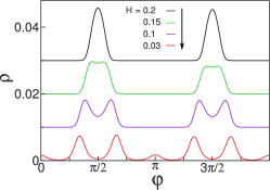
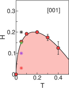
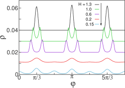
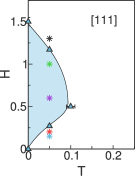
Figure 3: (Color online) Monte Carlo results for two field orientations $\mathbf{H}\parallel[001]$ (upper row) and $\mathbf{H}\parallel[111]$ (lower row). Left plots show histograms for the angle $\varphi$ collected at $T=0.05$. Histograms for larger fields are progressively offset by $\Delta\rho=0.01$. Right plots show phase diagrams in the relevant parts of the $H$–$T$ plane. Magnetic fields chosen for histograms are indicated by stars.

The MC results the low-$T$/low-$H$ region ($T_{c}\approx 0.79$, $H_{s}(0)\approx 6.45$) are summarized in Fig. 3. The transition with a loss of the mirror symmetry for ${\bf H}\parallel[001]$ is demonstrated by the behavior of the probability distribution function $\rho(\varphi)$ (upper left panel). At $H=0.2$ and $T=0.05$, $\rho(\varphi)$ has two sharp maxima corresponding to the $\psi_{3}$ states with $\varphi=\pi/2$ and $3\pi/2$. At a lower field $H=0.15$, each of them splits into a pair of peaks, which move further apart as $H$ is decreased. Using the Binder cumulant analysis we locate transition at $H_{c}=0.156(2)$ Suppl . The temperature dependence $H_{c}(T)$ is shown on the upper right plot. In the classical model, the order by disorder effect is present only at $T>0$ and the transition field vanishes as $T\to 0$. It goes down again for $T\to T_{c}$ since the six-fold anisotropy $E_{6}\propto m^{6}$ contains a higher power of the order parameter than the field contribution $E_{2}\propto m^{2}$.

Similarly, the case of ${\bf H}\parallel[111]$ is illustrated by two lower plots in Fig. 3. The intermediate low-symmetry phase is evidenced by split peaks in $\rho(\varphi)$ for $H=1$ and 0.6. The relevant part of the $H$–$T$ phase diagram is shown on the lower right plot. The broken-symmetry state is present only for $T\leq 0.1$. At higher temperatures, the six-fold anisotropy generated by thermal fluctuations is sufficiently strong to restore the $\psi_{2}$ states in the whole range of magnetic fields in accordance with the prior analytic treatment.

In conclusion, using analytic symmetry arguments we demonstrated that an external field applied to an $XY$ pyrochlore antiferromagnet induces two-, three- or six-fold clock terms that compete with the zero-field $Z_{6}$ anisotropy and produce a remarkably rich phase diagram. Our theory generalizes the concept of the spin-flop transition to magnetic systems with a discrete $Z_{N}$ anisotropy. Observation of such transitions is important for determining sign and strength of the six-fold clock anisotropy in $\rm Er_{2}Ti_{2}O_{7}$ and other $XY$ pyrochlores. In particular, presence of a low-field transition for ${\bf H}\parallel[001]$ but not for ${\bf H}\parallel[110]$ unambiguously places a pyrochlore magnet into the $J_{\perp}^{a}/J_{\perp}<4$ region of the parameter space ($J_{\pm\pm}>0$ in notations of Savary12 ) with the $\psi_{2}$ magnetic structure in zero field. The opposite behavior is expected for the $\psi_{3}$ ground state stabilized for $J_{\perp}^{a}/J_{\perp}>4$. These conclusions can be further corroborated by checking a number of field transitions in the ${\bf H}\parallel[111]$ geometry (Fig. 2). The obtained results call for additional magnetization and polarized neutron experiments on the $XY$ pyrochlores in a magnetic field.

SUPPLEMENTAL MATERIAL

I I. Extracting model parameters from magnetization curves

In $\rm Er_{2}Ti_{2}O_{7}$, the lowest Kramers doublet of Er³⁺ ions selected by the crystal field is separated from the next two levels by gaps of 6.38 and 7.39 meV Champion03s . Accordingly, the minimal spin model for this material applicable at low temperatures and weak magnetic fields can be formulated in terms of the pseudo spin-1/2 operators acting in the subspace of ground-state Kramers doublets. This assumption is corroborated by the recent heat-capacity measurements Niven14s ; Dalmas12s , which find a pronounced $R\ln 2$ plateau in the temperature dependence of the magnetic entropy $S_{\rm mag}(T)$ below 10 K. The effective nearest-neighbor Hamiltonian is a bilinear form of these spin-1/2 operators Zhitomirsky12s :

$$\hat{\cal H}=\sum_{\langle ij\rangle}\bigl{[}J_{\perp}{\bf S}^{\perp}_{i}\cdot{\bf S}^{\perp}_{j}+J_{\perp}^{a}({\bf S}^{\perp}_{i}\cdot\hat{\bf r}_{ij})({\bf S}^{\perp}_{j}\cdot\hat{\bf r}_{ij})\bigr{]}-\sum_{i}g_{\alpha\beta}\mu_{B}\,H^{\alpha}S_{i}^{\beta}\,.$$ (S1)

Here ${\bf S}^{\perp}_{i}$ are spin components perpendicular to the local trigonal axis $\hat{\bf z}_{i}$, $\hat{\bf r}_{ij}$ is a unit vector in the bond direction, and $g_{\alpha\beta}$ is a staggered $g$-tensor with the uniaxial symmetry:

$$g_{\alpha\beta}=g_{z}\hat{z}_{i}^{\alpha}\hat{z}_{i}^{\beta}+g_{\perp}\bigl{(}\delta_{\alpha\beta}-\hat{z}_{i}^{\alpha}\hat{z}_{i}^{\beta}\bigr{)}\,.$$ (S2)

In accordance with the $XY$ nature of the Er³⁺ magnetic moments, the effective Hamiltonian (S1) contains only planar components of spins. The omitted terms that include the $S_{i}^{z}$ components are smaller by about an order of magnitude Zhitomirsky12s ; Savary12s .

     

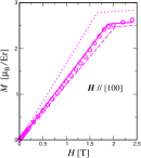
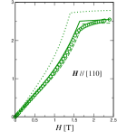
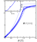
Figure 4: Magnetization of $\rm Er_{2}Ti_{2}O_{7}$ for three field orientations. Data points are the experimental results of Bonville et al. Bonville13s taken at $T=175$ mK ([100]) and 130 mK ([110] and [111]). The zero-temperature magnetization curves for the effective spin-1/2 Hamiltonian with the parameters given by Eq. (S3) are shown by the full lines. The dashed lines correspond to theoretical curves obtained with the parameters of Savary et al. Savary12s . The dotted lines are drawn for the set of coupling constants by Petit et al. Petit14s ; Cao09s . The inset on the right panel displays the field derivative $dM/dH$ in the low field region.

To fix parameters of the spin Hamiltonian (S1) we have fitted the low-temperature magnetization of $\rm Er_{2}Ti_{2}O_{7}$ reported by Bonville et al. Bonville13s . In all field orientations the measured $M(H)$ curves exhibit weak almost linear growth in a polarized paramagnetic state above the critical field $H_{s}\simeq 1.5$–1.7 T. We have subtracted this isotropic Van Vleck susceptibility $\chi_{V}/\textrm{Er}\approx 0.2\mu_{B}/\textrm{T}$ from the original experimental data. Magnetization in a given field has been computed for a classical spin configuration obtained by minimizing numerically the energy (S1) within the subspace of the four-sublattice magnetic structures. The experimental data together with our theoretical fits are shown in Fig. 4 for three field orientations. The microscopic parameters deduced from these fits are

$$J_{\perp}=0.2~{}\textrm{meV}\,,\quad J_{\perp}^{a}=0.3~{}\textrm{meV}\,,\quad g_{z}=3.0\,,\quad g_{\perp}=6.0\,.$$ (S3)

Previously, the exchange parameters of $\rm Er_{2}Ti_{2}O_{7}$ were obtained by Savary and coworkers Savary12s from the high-field INS measurements. They found $J_{\perp}=0.21(2)$ meV, $J^{a}_{\perp}=0.35(5)$ meV, $g_{z}=2.45\pm 0.23$ and $g_{\perp}=5.97\pm 0.08$ with two additional coupling constants $J_{zz}=-0.025(2)$ meV, $J_{z\perp}=0.03(5)$ meV omitted in the minimal spin model (S1). The corresponding magnetization curves are shown by dashed lines. An independent set of the coupling constants was derived by Petit et al. Petit14s from the zero-field INS experiments: $J_{\perp}=0.206$ meV, $J^{a}_{\perp}=0.308$ meV and also $J_{zz}=-0.022$ meV, $J_{z\perp}=0.052$ meV. Using the $g$-tensor values obtained earlier by the same group Cao09s , $g_{z}=2.6$ and $g_{\perp}=6.8$, we plot the resulting magnetization curves by dotted lines in Fig. 4. Overall, the three sets of microscopic parameters match each other within 10–15%. Nevertheless, our set (S3) demonstrates better agreement with the magnetization data justifying at the same time the use of the minimal spin model (S1).

The theoretical magnetization curve for ${\bf H}\parallel[111]$ in Fig. 4 exhibits a small but clear jump at the saturation field $H_{s}^{[111]}\approx 1.5$ T. This weak first-order transition into the polarized paramagnetic state is a direct consequence of the cubic invariant in the Landau energy functional for the $\Gamma_{5}$ order parameter given by Eq. (9) in the main text. The invariant vanishes for the two other field orientations leaving in those cases continuous second-order transitions at $H_{s}$.

The inset of the right panel of Fig. 4 shows the field derivative $dM/dH$ of the theoretical magnetization curve for ${\bf H}\parallel[111]$. A small jump in the derivative at $H_{c}\approx 0.4$ T indicates a second-order phase transition. We identify the anomaly with a transition between a low-symmetry state, Eq. (11) of the main text, and the $\psi_{2}$ states with $\varphi=\pi$ and $\pm\pi/3$ at high fields. Presence of such a transition can be easily understood on the basis of Eq. (10) in the main text with $A_{6}\equiv 0$, see also Sec. III below. This transition is present for all ratios of $J_{\perp}^{a}/J_{\perp}$ and is shown in Fig. 2 of the main text by a dotted line.

II II. Energy Correction in a weak magnetic field

Here we outline the analytic derivation and give complete expressions for the state-dependent energy corrections induced by a weak magnetic field. We adopt the following convention for the positions of magnetic atoms in the unit cell of a pyrochlore lattice

$$\mathbf{r}_{1}=(0,0,0)\,,\quad\mathbf{r}_{2}=(\tfrac{1}{4},\tfrac{1}{4},0)\,,\quad\mathbf{r}_{3}=(0,\tfrac{1}{4},\tfrac{1}{4})\,,\quad\mathbf{r}_{4}=(\tfrac{1}{4},0,\tfrac{1}{4})\,.\quad$$ (S4)

The local coordinate frame for each site is defined by the set of basis vectors

$$\mathbf{\hat{x}}_{1}=\frac{1}{\sqrt{6}}(1,1,-2)\,,\ \mathbf{\hat{x}}_{2}=\frac{1}{\sqrt{6}}(-1,-1,-2)\,,\ \mathbf{\hat{x}}_{3}=\frac{1}{\sqrt{6}}(1,-1,2)\,,\ \mathbf{\hat{x}}_{4}=\frac{1}{\sqrt{6}}(-1,1,2)\,,$$

$$\mathbf{\hat{y}}_{1}=\tfrac{1}{\sqrt{2}}(-1,1,0)\,,\ \mathbf{\hat{y}}_{2}=\frac{1}{\sqrt{2}}(1,-1,0)\,,\ \mathbf{\hat{y}}_{3}=\frac{1}{\sqrt{2}}(-1,-1,0)\,,\ \mathbf{\hat{y}}_{4}=\frac{1}{\sqrt{2}}(1,1,0)\,,$$ (S5)

$$\hat{\bf z}_{1}=\frac{1}{\sqrt{3}}(1,1,1)\,,\ \hat{\bf z}_{2}=\frac{1}{\sqrt{3}}(-1,-1,1)\,,\ \hat{\bf z}_{3}=\frac{1}{\sqrt{3}}(1,-1,-1)\,,\ \hat{\bf z}_{4}=\frac{1}{\sqrt{3}}(-1,1,-1)\,.\$$

The $\hat{\bf x}_{i}$ and $\hat{\bf y}_{i}$ axes coincide with spin directions in the $\psi_{2}$ and $\psi_{3}$ magnetic structures, respectively, see Fig. 1 of the main text. The degenerate $E$ ($\Gamma_{5}$) manifold of ground-state spin configurations can be parameterized by a single angle: $\mathbf{S}_{i}=\hat{\bf x}_{i}\cos\varphi+\hat{\bf y}_{i}\sin\varphi$. Expansion of the Hamiltonian (S1) in small deviations from a classical ground state was performed in Ref. Maryasin14s . Keeping only terms that are quadratic in in-plane, $\mathsf{S}^{y}_{i}$, and out-of-plane, $\mathsf{S}^{z}_{i}$, spin components we rewrite (S1) as

$$\hat{\cal H}_{2}=\frac{h}{2S}\sum_{i}\left[\mathsf{S}_{i}^{z}{}^{2}+\mathsf{S}_{i}^{y}{}^{2}\right]-2\sum_{\langle ij\rangle}M_{ij}\,\mathsf{S}_{i}^{y}\,\mathsf{S}_{j}^{y}\,;\qquad i,j=1\ldots 4\,,$$ (S6)

where $h=(2J_{\perp}+J_{\perp}^{a})S$ is a site-independent amplitude of the local magnetic field and $M_{ij}$ is a set of bond-dependent coupling constants

$$M_{ij}=\frac{1}{6}\,(2J_{\perp}+J_{\perp}^{a})+\frac{1}{6}\,(4J_{\perp}-J_{\perp}^{a})\cos(2\varphi+\gamma_{ij})\,,$$

$$\gamma_{12}=\gamma_{34}=0\,,\qquad\gamma_{13}=\gamma_{24}=\frac{2\pi}{3}\,,\qquad\gamma_{14}=\gamma_{23}=-\frac{2\pi}{3}\,.$$ (S7)

An external magnetic field adds linear terms to $\hat{\cal H}_{2}$, which distort the magnetic structure. In the rotated local frame the Zeeman energy becomes

$$\hat{\cal H}_{Z}=-\sum_{i}\left[g_{z}\mu_{B}H_{i}^{z}\mathsf{S}_{i}^{z}+g_{\perp}\mu_{B}H_{i}^{\perp}\mathsf{S}_{i}^{y}\sin(\varphi-\phi_{i})+O(\mathsf{S}_{i}^{2})\right],$$ (S8)

where $\phi_{i}$ is an angle between the in-plane component of the applied field and the $\hat{\bf x}_{i}$ spin axis. Explicitly, the in-plane field components $H^{\perp}_{i}$ and the polar angles $\phi_{i}$ are given for the three field orientations by

$$H \ \parallel[001] H \ \parallel[110] H \ \parallel[111]$$

$$H_{1}^{\perp} =\sqrt{\tfrac{2}{3}}H; \phi_{1} =\pi;\qquad\qquad H_{1}^{\perp} =\tfrac{1}{\sqrt{3}}H; \phi_{1} =0;\qquad\qquad H_{1}^{\perp} =0;$$

$$H_{2}^{\perp} =\sqrt{\tfrac{2}{3}}H; \phi_{2} =\pi;\qquad\qquad H_{2}^{\perp} =\tfrac{1}{\sqrt{3}}H; \phi_{2} =\pi;\qquad\qquad H_{2}^{\perp} =\tfrac{\sqrt{8}}{3}H; \phi_{2} =\pi;$$ (S9)

$$H_{3}^{\perp} =\sqrt{\tfrac{2}{3}}H; \phi_{3} =0;\qquad\qquad H_{3}^{\perp} =H; \phi_{3} =-\pi/2;\qquad\qquad H_{3}^{\perp} =\tfrac{\sqrt{8}}{3}H; \phi_{3} =-\pi/3;$$

$$H_{4}^{\perp} =\sqrt{\tfrac{2}{3}}H; \phi_{4} =0;\qquad\qquad H_{4}^{\perp} =H; \phi_{4} =\pi/2;\qquad\qquad H_{4}^{\perp} =\tfrac{\sqrt{8}}{3}H; \phi_{4} =\pi/3.$$

Since the terms containing $\mathsf{S}^{z}_{i}$ in Eqs. (S6) and (S8) are $\varphi$-independent, the out-of-plane deviations do not affect the ground state degeneracy at quadratic order in $H$. To minimize over the in-plane fluctuations $\mathsf{S}^{y}_{i}$ we first diagonalize of the quadratic form (S6) with the help of a suitable orthogonal transformation:

$$T=\frac{1}{2}\begin{pmatrix}-1&-1&\;\;\,1&1\\ -1&\;\;\,1&-1&1\\ \;\;\,1&-1&-1&1\\ \;\;\,1&\;\;\,1&\;\;\,1&1\end{pmatrix}.$$ (S10)

The eigenvalues $\Lambda=\rm{diag}\{\lambda_{1};\lambda_{2};\lambda_{3};\lambda_{4}\}$ calculated as $\Lambda=T^{-1}MT$ are given by

$$\lambda_{n}=\frac{2}{3}(2J_{\perp}+J_{\perp}^{a})-\frac{1}{3}(4J_{\perp}-J_{\perp}^{a})\cos(2\varphi+\gamma_{1\,n+1})\,,\ \ n=1\!-\!3\,,\qquad\lambda_{4}=0\,.$$ (S11)

The zero eigenmode $\lambda_{4}$ corresponds to motion of spins inside the degenerate ground-state manifold and does not contribute to the degeneracy lifting. The energy correction is, then, obtained by direct minimization of the diagonal quadratic form and the linear terms:

$$\Delta E=-\frac{(g_{\perp}\mu_{B})^{2}}{4}\frac{N}{4}\sum_{n=1}^{3}\frac{\Bigl{(}\sum_{k=1}^{4}H_{k}^{\perp}\sin(\varphi-\phi_{k})t_{kn}\Bigr{)}^{2}}{\lambda_{n}}\,.$$ (S12)

Here $t_{kn}$ are elements of the transformation matrix $T$ and the normalization factor $N/4$ extends the result to the entire lattice with $N$ spins. Full expressions for the $\varphi$-dependent energy terms quadratic in a weak magnetic field $H$ are obtained by substituting $H^{\perp}_{k}$ and $\phi_{k}$ from Eq. (S9).

For a magnetic field applied along the $[001]$ axis, the field-induced energy correction is given by

$$\Delta E^{[001]}=\frac{(g_{\perp}\mu_{B}H)^{2}N}{8(2J_{\perp}+J_{\perp}^{a})}\ \frac{\cos 2\varphi-1}{1-\epsilon\cos 2\varphi}\,,$$ (S13)

where $\epsilon$ is a dimensionless parameter $\epsilon=(J_{\perp}-J_{\perp}^{a}/4)/(J_{\perp}+J_{\perp}^{a}/2)$. In the parameter region spanned by positive exchange constants $J_{\perp}$ and $J_{\perp}^{a}$, the variations of $\epsilon$ are restricted to $-0.5<\epsilon<1$. In particular, for $\rm Er_{2}Ti_{2}O_{7}$ we obtain $\epsilon\approx 0.36$. Thus, for all relevant $\epsilon$, the energy correction remains finite and selects states with $\varphi=\pm\pi/2$. The expression for $\Delta E^{[001]}$ presented in the main text corresponds to $\epsilon=0$. To achieve a better accuracy one may use the full expression (S13).

For $\mathbf{H}\parallel[110]$ the field-induced anisotropy has a more complex expression

$$\Delta E^{[110]}=-\frac{(g_{\perp}\mu_{B}H)^{2}N}{16(2J_{\perp}+J_{\perp}^{a})}\ \frac{2-\epsilon/2+(\epsilon+1)\cos 2\varphi+\epsilon\cos 4\varphi}{1-\epsilon^{2}/4+\epsilon\cos 2\varphi+(\epsilon^{2}/2)\cos 4\varphi}\,.$$ (S14)

Still, a simple analysis shows that the field contribution is finite for all $\epsilon$ and selects states with $\varphi=0,\pi$ (see also below). The amplitude of the $2\varphi$ harmonic exactly equals $-1/2$ the corresponding result for $\mathbf{H}\parallel[001]$.

Finally, the quadratic energy correction for $\mathbf{H}\parallel[111]$ is

$$\Delta E^{[111]}=\frac{(g_{\perp}\mu_{B}H)^{2}N}{8(2J_{\perp}+J_{\perp}^{a})}\ \frac{-4+2\epsilon+\epsilon^{2}+\epsilon^{2}\cos 6\varphi}{1-3\epsilon^{2}/4-(\epsilon^{3}/4)\cos 6\varphi}\,.$$ (S15)

As before, the denominator does not vanish, ensuring a finite energy shift, and the selection term is proportional to $\cos 6\varphi$ with a positive coefficient. The obtained analytic expressions for all three field directions were checked against direct numerical minimization of the classical energy (S1) in the four-sublattice basis and full agreement was found for weak magnetic fields $H\ll H_{s}$. In addition, the numerical minimization confirms a change of sign of the $4\varphi$ harmonic in the expression (S14) for negative $\epsilon$. While the prefactor of $\cos 2\varphi$ is always negative, the coefficient of $\cos 4\varphi$ becomes positive for $J^{\perp}_{a}/J_{\perp}>4$ ($\epsilon<0$). The sign change can modify stability of the two domains with $\varphi=0,\pi$ predicted by the symmetry analysis. Indeed, more complex spin configurations were found in our simulations for $J_{\perp}^{a}/J_{\perp}\gtrsim 10$. Though this case is far beyond the parameter range expected for $\mathrm{Er_{2}Ti_{2}O_{7}}$, it still might be relevant for another pyrochlore material, $\mathrm{Er_{2}Ge_{2}O_{7}}$, which was suggested to order in the $\psi_{3}$ state Dun15s .

III III. Field-induced orientational transitions

Using the third-order real-space perturbation theory we obtained the following expression for the $Z_{6}$ anisotropy Maryasin14s :

$$E_{6}(\varphi)=-\frac{2J_{\perp}+2J_{\perp}^{a}}{10^{3}}\,\epsilon^{3}\,(1+\tfrac{1}{4}\epsilon^{2})\cos 6\varphi\,.$$ (S16)

Besides spin-flip hopping processes, this expression takes into account the effect of spin-flip interaction. Interactions reduce by $\sim 40$ % the amplitude of the six-fold harmonics in comparison with the harmonic spin-wave result. We consider the above expression to be more accurate, though the approximate nature of all analytic expressions for the quantum anisotropy must be kept in mind.

In order to determine the transition fields for ${\bf H}\parallel[001]$ and $[110]$ we use complete expressions for the field-induced anisotropy terms (S13) and (S14) together with the quantum contribution (S16). By checking the stability of the high-field state with $\varphi=\pi/2$ we obtain:

$$g_{\perp}\mu_{B}H_{c}^{[001]}=\frac{3}{5}(2J_{\perp}+J_{\perp}^{a})\epsilon(1+\epsilon)\sqrt{\frac{\epsilon(1+\tfrac{1}{4}\epsilon^{2})}{5(1-\epsilon)}\,}\,.$$ (S17)

It applies for $\epsilon>0$ or $J_{\perp}^{a}/J_{\perp}<4$. Numerical results obtained with this expression are shown in top-left panel of Fig. 2 of the main text.

A similar calculation for the stability of the state with $\varphi=\pi$ yields

$$g_{\perp}\mu_{B}H_{c}^{[110]}=\frac{6}{5}(2J_{\perp}+J_{\perp}^{a})|\epsilon|(1+\epsilon/2)\sqrt{\frac{|\epsilon|(1+\tfrac{1}{4}\epsilon^{2})(1+\tfrac{1}{2}\epsilon)}{10(1-\epsilon)(1+\tfrac{7}{2}\epsilon)}\,}\,.$$ (S18)

This expression holds for $-2/7\leq\epsilon\leq 0$ or $4\leq J_{\perp}^{a}/J_{\perp}\leq 12$, the corresponding curve is drawn of the top-right panel of Fig. 2 of the main text. For $\epsilon\to-2/7$, the above expression diverges, which means that $H_{c}^{[110]}$ approaches the saturation field $H_{s}$. Beyond this range for $\epsilon<-\tfrac{2}{7}$, the $\psi_{2}$ states do not appear in a magnetic field and the low-symmetry states occupy the whole range of magnetic fields $0<H<H_{s}$.

Finally, for ${\bf H}\parallel[111]$, in addition to the contribution (S15), an external magnetic field also generates a three-fold harmonic in the angular-dependant part of energy (see the main text):

$$E_{3}(\varphi)=\lambda_{3}\frac{(g_{\perp}\mu_{B}H)^{3}}{(2J_{\perp}+J_{\perp}^{a})^{2}}\,\cos 3\varphi\,.$$ (S19)

The dimensionless factor $\lambda_{3}$ cannot be expressed analytically. Therefore, we proceed with calculations in the two-step manner. First, we consider only $E_{3}(\varphi)$ and (S15) contributions. Their competition produces a single transition exhibited by the classical model at zero-temperature, i.e., in the absence of the zero-field six-fold anisotropy:

$$g_{\perp}\mu_{B}H_{c}^{[111]}=(2J_{\perp}+J_{\perp}^{a})\frac{2\epsilon^{2}(2-\epsilon)}{\lambda_{3}(1-\epsilon)(2+\epsilon)^{3}}\,.$$ (S20)

Numerical differentiation of the calculated magnetization curves is used to determine the position of this transition for all values of $J_{\perp}^{a}/J_{\perp}$, an example is given in the inset of Fig. 1. This allows us to estimate the dimensionless amplitude $\lambda_{3}$ of the three-fold harmonic as a function of $J_{\perp}^{a}/J_{\perp}$. Second, we add the zero-field term (S16) and use the numerical values of $\lambda_{3}$ to solve the cubic equation obtained by determining the stability of the state with $\varphi=\pi$. Depending on the coefficients, there are either no or two positive real roots of that equation for $\epsilon>0$, whereas for $\epsilon<0$ the cubic equation has always one positive root. The obtained numerical results are used for Fig. 2 of the main text.

IV IV. Classical Monte Carlo simulations

             

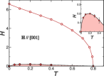
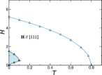
Figure 5: Monte Carlo phase diagrams of the $XY$ pyrochlore antiferromagnet for two orientations of an applied magnetic field.

Monte Carlo simulations of the classical model (S1) were performed using a hybrid algorithm, which consists of a combination of single spin Monte Carlo updates with microcanonical overrelaxation steps Zhitomirsky12s ; Maryasin14s ; Zhitomirsky14s . Periodic clusters with $N=4L^{3}$ spins up to $L=24$ were simulated. Majority of Monte Carlo runs were performed at fixed $T$ starting with a random initial spin configuration at a large enough field $H>H_{s}$, and decreasing gradually the field strength. Statistical averages were taken over 300 independent runs, each measurement was taken during up to $2\cdot 10^{5}$ Monte Carlo steps and the first $5\cdot 10^{4}$ steps at each field were omitted for thermalization.

The transition from the paramagnetic to the ordered phase was determined with the help of the $\Gamma_{5}$-representation order parameter

$$m=\sqrt{m_{1}^{2}+m_{2}^{2}},\qquad\qquad m_{1}=\frac{1}{N}\sum_{i}\mathbf{S}_{i}\cdot\mathbf{\hat{x}}_{i},\qquad m_{2}=\frac{1}{N}\sum_{i}\mathbf{S}_{i}\cdot\mathbf{\hat{y}}_{i}.$$ (S21)

Different antiferromagnetic ordered phases were distinguished by simultaneously measuring the clock-type order parameters $m_{p}^{\prime}$, $m_{p}^{\prime\prime}$

$$m_{p}^{\prime}=\frac{1}{m^{p-1}}{\rm Re}\{(m_{1}+im_{2})^{p}\}=m\cos p\varphi;\qquad\qquad m_{p}^{\prime\prime}=\frac{1}{m^{p-1}}{\rm Im}\{(m_{1}+im_{2})^{p}\}=m\sin p\varphi$$ (S22)

with $p=2,3,6$. Finally, the corresponding Binder cumulants $U(m_{p})=1-\langle m_{p}^{4}\rangle/3\langle m_{p}^{2}\rangle^{2}$ were used for precise determination of the phase boundaries.

           

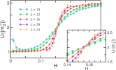
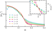
Figure 6: Finite-size analysis of the orientational transition for $\mathbf{H}\parallel[001]$ at $T=0.05$. Left panel: field dependence of the Binder cumulants for the $m_{2}^{\prime\prime}$ order parameter for different cluster sizes. Their crossing defines the transition field $H_{c}=0.156(2)$. Right panel: field dependence of the order parameter $|m_{2}^{\prime\prime}|$. The inset illustrates the procedure for determining the $\beta/\nu$ value. The best crossing is obtained for $\beta/\nu\approx 0.7$.

The spin Hamiltonian parameters adopted in the simulations are $J_{\perp}=1$, $J_{\perp}^{a}=1.5$, $g_{\perp}=1$, $g_{z}=0.5$ in accordance with the magnetization fits (Sec. I). Complete phase diagrams for the two field orientations $\mathbf{H}\parallel[001]$ and $\mathbf{H}\parallel[111]$ are shown in Fig. 5. The zero-field transition temperature is $T_{c}=0.793(2)$ for this set of exchange parameters Zhitomirsky14s . Nontrivial phases are denoted by color shading. Phase transitions are second order except for the PM-AFM phase boundary for $\mathbf{H}\parallel[111]$. The latter boundary is a line of first-order phase transitions with a small discontinuous jump in the magnetization, although the discontinuity is barely observable for $T\gtrsim 0.2$.

Figure 6 illustrates the finite-size analysis used to determine the boundary $H_{c}(T)$ of the orientational transition for ${\bf H}\parallel[001]$. Temperature is set to $T=0.05$. The transition field $H_{c}=0.156(2)$ is determined from the crossing of the Binder cumulants for different cluster sizes (left panel). The right panel shows the field dependence of the order parameter $|m_{2}^{\prime\prime}|$ and the inset illustrates the scaling procedure used to obtain an estimate for the critical exponent ratio $\beta/\nu=0.70(5)$. This value is obtained by searching for the best crossing of the scaled order parameters $|m_{2}^{\prime\prime}|L^{\beta/\nu}$ at the same critical field $H_{c}$ upon varying $\beta/\nu$. It differs from the value $\beta/\nu=0.518$ for the Ising universality class in three dimensions. The origin for such a substantial discrepancy is not clear at present. Most probably it is due to the fact that the six-fold anisotropy is dangerously irrelevant in 3D, see, e.g., Zhitomirsky14s and thus the correct scaling behavior is only obtained for significantly larger lattices.

References

• (1) P. M. Chaikin and T. C. Lubensky, Principles of condensed matter physics, (Cambridge University Press, Cambridge, 1995).
• (2) E. Schneidman, M. J. Berry, R. Segev, and W. Bialek, Nature 440, 1007 (2006).
• (3) J. V. JosΓ©, L. P. Kadanoff, S. Kirkpatrick, and D. R. Nelson, Phys. Rev. B 16, 1217 (1977).
• (4) J. D. M. Champion, M. J. Harris, P. C. W. Holdsworth, A. S. Wills, G. Balakrishnan, S. T. Bramwell, E. Cizmar, T. Fennell, J. S. Gardner, J. Lago, D. F. McMorrow, M. Orendac, A. Orendacova, D. McK. Paul, R. I. Smith, M. T. F. Telling, and A. Wildes, Phys. Rev. B 68, 020401(R) (2003).
• (5) J. D. M. Champion and P. C. W. Holdsworth, J. Phys.: Condens. Matter 16, S665 (2004).
• (6) A. Poole, A. S. Wills, and E. LeliΓ¨vre-Berna, J. Phys.: Condens. Matter 19, 452201 (2007).
• (7) M. E. Zhitomirsky, M. V. Gvozdikova, P. C. W. Holdsworth, and R. Moessner, Phys. Rev. Lett. 109, 077204 (2012).
• (8) L. Savary, K. A. Ross, B. D. Gaulin, J. P. C. Ruff, and L. Balents, Phys. Rev. Lett. 109, 167201 (2012).
• (9) A. W. C. Wong, Z. Hao, and M. J. P. Gingras, Phys. Rev. B 88, 144402 (2013).
• (10) H. Yan, O. Benton, L. Jaubert, and N. Shannon, arXiv:1311.3501.
• (11) M. E. Zhitomirsky, P. C. W. Holdsworth, and R. Moessner, Phys. Rev. B 89, 140403(R) (2014).
• (12) K. A. Ross, Y. Qiu, J. R. D. Copley, H. A. Dabkowska, and B. D. Gaulin, Phys. Rev. Lett. 112, 057201 (2014).
• (13) P. A. McClarty, P. Stasiak, and M. J. P. Gingras, Phys. Rev. B 89, 024425 (2014).
• (14) S. Petit, J. Robert, S. Guitteny, P. Bonville, C. Decorse, J. Ollivier, H. Mutka, M. J. P. Gingras, and I. Mirebeau, Phys. Rev. B 90, 060410(R) (2014).
• (15) B. Javanparast, A. G. R. Day, Z. Hao, and M. J. P. Gingras, Phys. Rev. B 91, 174424 (2015).
• (16) X. Li, W. M. Li, K. Matsubayashi, Y. Sato, C. Q. Jin, Y. Uwatoko, T. Kawae, A. M. Hallas, C. R. Wiebe, A. M. Arevalo-Lopez, J. P. Attfield, J. S. Gardner, R. S. Freitas, H. D. Zhou, and J.-G. Cheng, Phys. Rev. B 89, 064409 (2014).
• (17) Z. L. Dun, X. Li, R. S. Freitas, E. Arrighi, C. R. Dela Cruz, M. Lee, E. S. Choi, H. B. Cao, H. J. Silverstein, C. R. Wiebe, J. G. Cheng, and H. D. Zhou, Phys. Rev. B 92, 140407(R) (2015).
• (18) N. Majlis, The quantum theory of magnetism, (World Scientific, Singapore, 2007).
• (19) P. A. McClarty, S. H. Curnoe, and M. J. P. Gingras, J.Β Phys. Conf. Ser. 145, 012032 (2009).
• (20) J. G. Rau, S. Petit, and M. J. P. Gingras, arXiv: 1510.04292.
• (21) L. Savary and L. Balents, Phys. Rev. Lett. 108, 037202 (2012).
• (22) P. Bonville, S. Petit, I. Mirebeau, J. Robert, E. Lhotel, and C. Paulsen, J. Phys.: Condens. Matter 25, 275601 (2013).
• (23) see Supplemental Material.
• (24) V. S. Maryasin and M. E. Zhitomirsky, Phys. Rev. B 90, 094412 (2014).
• (25) J. P. C. Ruff, J. P. Clancy, A. Bourque, M. A. White, M. Ramazanoglu, J. S. Gardner, Y. Qiu, J. R. D. Copley, M. B. Johnson, H. A. Dabkowska, and B. D. Gaulin, Phys. Rev. Lett. 101, 147205 (2008).
• (26) H. B. Cao, I. Mirebeau, A. Gukasov, P. Bonville, and C. Decorse, Phys. Rev. B 82, 104431 (2010).

References

• (1) J. D. M. Champion, M. J. Harris, P. C. W. Holdsworth, A. S. Wills, G. Balakrishnan, S. T. Bramwell, E. Cizmar, T. Fennell, J. S. Gardner, J. Lago, D. F. McMorrow, M. Orendac, A. Orendacova, D. McK. Paul, R. I. Smith, M. T. F. Telling, and A. Wildes, Phys. Rev. B 68, 020401(R) (2003).
• (2) J. F. Niven, M. B. Johnson, A. Bourque, P. J. Murray, D. D. James, H. A. Dabkowska, B. D. Gaulin, and M. A. White, Proc. R. Soc. A 470, 20140387 (2014).
• (3) P. Dalmas de RΓ©otier, A. Yaouanc, Y. Chapuis, S. H. Curnoe, B. Grenier, E. Ressouche, C. Marin, J. Lago, C. Baines, and S. R. Giblin, Phys. Rev. B 86, 104424 (2012).
• (4) M. E. Zhitomirsky, M. V. Gvozdikova, P. C. W. Holdsworth, and R. Moessner, Phys. Rev. Lett. 109, 077204 (2012).
• (5) L. Savary, K. A. Ross, B. D. Gaulin, J. P. C. Ruff, and L. Balents, Phys. Rev. Lett. 109, 167201 (2012).
• (6) P. Bonville, S. Petit, I. Mirebeau, J. Robert, E. Lhotel, and C. Paulsen, J. Phys.: Condens. Matter 25, 275601 (2013).
• (7) S. Petit, J. Robert, S. Guitteny, P. Bonville, C. Decorse, J. Ollivier, H. Mutka, M. J. P. Gingras, and I. Mirebeau, Phys. Rev. B 90, 060410(R) (2014).
• (8) H. Cao, A. Gukasov, I. Mirebeau, P. Bonville, C. Decorse, and G. Dhalenne, Phys. Rev. Lett. 103, 056402 (2009).
• (9) V. S. Maryasin and M. E. Zhitomirsky, Phys. Rev. B 90, 094412 (2014).
• (10) Z. L. Dun, X. Li, R. S. Freitas, E. Arrighi, C. R. Dela Cruz, M. Lee, E. S. Choi, H. B. Cao, H. J. Silverstein, C. R. Wiebe, J. G. Cheng, and H. D. Zhou, Phys. Rev. B 92, 140407(R) (2015).
• (11) M. E. Zhitomirsky, P. C. W. Holdsworth, and R. Moessner, Phys. Rev. B 89, 140403(R) (2014).